Landsat 15-m Panchromatic-Assisted Downscaling (LPAD) of the 30-m Reflective Wavelength Bands to Sentinel-2 20-m Resolution

Abstract

The Landsat 15-m Panchromatic-Assisted Downscaling (LPAD) method to downscale Landsat-8 Operational Land Imager (OLI) 30-m data to Sentinel-2 multi-spectral instrument (MSI) 20-m resolution is presented. The method first downscales the Landsat-8 30-m OLI bands to 15-m using the spatial detail provided by the Landsat-8 15-m panchromatic band and then reprojects and resamples the downscaled 15-m data into registration with Sentinel-2A 20-m data. The LPAD method is demonstrated using pairs of contemporaneous Landsat-8 OLI and Sentinel-2A MSI images sensed less than 19 min apart over diverse geographic environments. The LPAD method is shown to introduce less spectral and spatial distortion and to provide visually more coherent data than conventional bilinear and cubic convolution resampled 20-m Landsat OLI data. In addition, results for a pair of Landsat-8 and Sentinel-2A images sensed one day apart suggest that image fusion should be undertaken with caution when the images are acquired under different atmospheric conditions. The LPAD source code is available at GitHub for public use.

1. Introduction

The Landsat-8 polar-orbiting satellite (launched 2013) carries the Operational Land Imager (OLI) that has nine reflective wavelength (435 nm to 1384 nm) spectral bands; eight 30-m visible, near-infrared, short wave infrared, and cirrus bands, and also one 15-m panchromatic band [1]. The multi-spectral instrument (MSI) onboard the Sentinel-2A (launched 2015) and Sentinel-2B (launched 2017) polar-orbiting satellites acquires multi-spectral reflective wavelength medium resolution data with a design heritage from the Landsat and Satellite Pour l’Observation de la Terre (SPOT) sensors [2]. The MSI has 13 reflective wavelength (443 nm to 2190 nm) spectral bands; four 10-m visible and near-infrared bands, six 20-m red edge, near-infrared and short wave infrared bands, and three 60-m bands. Combination of near-contemporaneous Landsat-8 OLI and Sentinel-2 MSI data will provide increased opportunities for more frequent cloud-free surface observations [3,4]. For example, recent research suggests that the integration of the Landsat-8 and Sentinel-2 data would be beneficial for applications including agricultural mapping and monitoring [5,6,7], phenological studies [8], and glacier extent mapping [9]. There are a number of pre-processing issues that need to be addressed before the well calibrated Landsat-8 [10,11] and Sentinel-2A [2,12] data can be used together or treated as effectively being sensed from the same sensor. These include handling the different sensor spectral response functions and correction for atmospheric effects [13,14], correction of surface reflectance anisotropy [15,16], and handling image tiling and geolocation differences [17,18,19].

This paper is concerned with the Landsat-8 and Sentinel-2 spatial resolution differences. The different Landsat-8 and Sentinel-2 spatial resolutions can be overcome by reprojecting their data into the same coordinate system and then upscaling or downscaling the data from one sensor to the other. The Sentinel-2 10-m and 20-m data could be upscaled to match the Landsat-8 30-m data. For example, by resampling the 10-m and 20-m Sentinel-2 bands to Landsat 30-m resolution for sensor comparison of spectral indices [20] or to derive between-sensor registration information [21]. Conversely, the Landsat-8 30-m data could be downscaled to match the Sentinel-2 20-m or 10-m data. For example, by resampling the Landsat-8 30-m data to Sentinel-2 resolution for applications including agriculture monitoring [7], land cover classification [22], glacier extent mapping [9], or to derive between-sensor registration information [18]. Downscaling of Landsat-8 30-m data to the Sentinel-2 20-m or 10-m resolution is attractive as the more spatially resolved Sentinel-2 information is not lost.

In this paper a new method to downscale the Landsat-8 30-m bands to Sentinel-2A 20-m resolution is presented and compared to conventional resampling approaches. The Landsat 15-m Panchromatic-Assisted Downscaling (LPAD) method has two principal steps: (i) downscaling the Landsat-8 30-m reflective band data to 15-m resolution using the detailed spatial information provided by the Landsat-8 15-m panchromatic band and then (ii) reprojecting and resampling the downscaled 15-m data into registration with the Sentinel-2A 20-m data. It is shown to introduce less spectral and spatial distortion and to provide visually more coherent data than conventionally resampled Landsat 20-m data for pairs of images selected on the same day over diverse environments. In addition, results for Landsat-8 and Sentinel-2A images sensed one day apart are included and suggest that fusion of these sensor data should be undertaken with caution when they are acquired under different atmospheric conditions. The LPAD source code is made available at GitHub for public use.

2. Data and Study Areas

The Landsat-8 satellite was launched February 2013 and carries the OLI and Thermal Infrared Sensor (TIRS) that sense the Earth’s land surface with a 16 day repeat cycle over a 185-km-wide swath acquired from a sun-synchronous polar orbit [1,23]. The TIRS has two 100-m thermal bands but unfortunately a stray-light issue means that they are sub-optimal and land surface temperature retrieval using split-window techniques is not recommended [24]. The Sentinel-2A MSI was launched June 2015 and the follow on Sentinel-2B MSI was launched March 2017 and each has a 10-day repeat cycle and together a five-day repeat cycle and provide 290-km-wide swaths from sun-synchronous orbits [2]. Both the OLI and MSI sensors have 12-bit radiometric resolution.

Table 1. Landsat-8 OLI and Sentinel-2 MSI equivalent spectral bands [2,23] considered in this study.

Landsat-8			Sentinel-2
Band	Resolution (m)	Wavelength Range (nm)	Band	Resolution (m)	Wavelength Range (nm)
B2 (Blue)	30	452–512	B2	10	458–523
B3 (Green)	30	533–590	B3	10	543–578
B4 (Red)	30	636–673	B4	10	650–680
B5 (NIR)	30	851–879	B8A	20	855–875
B6 (SWIR-1)	30	1566–1651	B11	20	1565–1655
B7 (SWIR-2)	30	2107–2294	B12	20	2100–2280
B8 (Pan)	15	503–676	-	-	-

shows the OLI and spectrally equivalent MSI reflective wavelength bands used in this study. The shortest wavelength sensor blue bands were not used because they are particularly sensitive to atmospheric effects [13,25]. The 30-m OLI cirrus (1363–1384 nm) band and the three 60-m MSI bands (433–453 nm, 935–955 nm, and 1360–1390 nm) were not used because they are primarily designed for atmospheric remote sensing [1,2].

Five pairs of contemporaneous Landsat-8 and Sentinel-2A images over sites with different land cover and containing anthropogenic and natural features with straight and irregular boundaries were selected (

Table 2. Landsat-8 (L8) and Sentinel-2A (S2A) study data.

Land Cover Type	Geographic Location	L8 Path/Row	S2A Tile	Acquisition Date	Acquisition Time (HH:MM:SS)
Urban area	New York, USA	14/32	18TWL	15 October 2016	L8: 15:40:12.12 S2A: 15:45:19.85
Crop field	California, USA	43/34	10SFG	23 August 2016	L8: 18:40:01.87 S2A: 18:57:15.69
Burned forest	California, USA	41/35	11SLV	26 September 2016	L8: 18:28:10.06 S2A: 18:38:51.43
Mountain landslides	Kaikoura, New Zealand	73/89	59GQP	15 December 2016	L8: 22:07:29.99 S2A: 22:25:39.46
Tropical forest	Makanra, Democratic Republic of the Congo	180/58	34NBH	L8: 3 March 2017 S2A: 4 March 2017	L8: 08:55:59.42 S2A: 09:10:10.15

, images illustrated in Section 4). The five sites include urban areas, crop fields, burned areas, landslides, and tropical forest, and were sensed under cloud-free conditions. Four of the image pairs were selected so that the Landsat-8 and Sentinel-2A images were sensed on the same day (from only about 5 min to 19 min apart) in order to minimize the impact of land surface and atmospheric changes. Consequently, none of the image data were atmospherically corrected. The Congo image pair was selected because the sensor data were acquired one day apart and the Sentinel-2A image contained evident smoke aerosols due to biomass burning. The impact of land surface and atmospheric changes on the Congo image pair is discussed in Section 6.

The recently available Landsat-8 Collection 1 Tier-1 OLI data, that are geolocated with a radial root mean square error <12 m and have a band-to-band registration accuracy less than 4.5 m [1,26], were used. The data are available in approximately 185 km × 180 km scenes defined in the Universal Transverse Mercator (UTM) projection and in the heritage Worldwide Reference System (WRS-2) of path (ground track parallel) and row (latitude parallel) coordinates [27]. The stored Landsat-8 digital numbers were converted to top of atmosphere (TOA) spectral reflectance (${\rho }_{\lambda }$, unitless) using metadata conversion coefficients and then dividing by the sine of the scene center solar elevation angle (${\theta }_s$). Sentinel-2A L1C data that are available in 109 km × 109 km tiles with the UTM projection and US Military Grid Reference System (MGRS) [17,28] were used. The Sentinel-2A L1C data have geo-location accuracy specifications of less than 12.5 m and band-to-band registration accuracies of less than 3 m, 6 m, and 18 m for the 10-m, 20-m, and 60-m bands, respectively [29].

3. Landsat 15-m Panchromatic-Assisted Downscaling (LPAD)

The LPAD method consists of two principal steps: (i) downscaling the Landsat-8 30-m reflective band data to 15-m resolution using the detailed spatial information provided by the Landsat-8 15-m panchromatic band and then (ii) reprojecting and resampling the downscaled 15-m data into registration with the Sentinel-2A 20-m data. These steps are described below.

3.1. Downscaling Landsat-8 30-m Data to 15 m Using the Panchromatic Band

Downscaling is a process to enhance the spatial resolution of sensor data usually by using information provided by other higher resolution ancillary data [30,31,32,33,34]. It is sometimes termed data fusion, or more specifically, pansharpening, when the higher resolution ancillary data is the panchromatic band [35,36,37,38,39]. Hereafter, for consistency, the term downscaling is used throughout this paper. Downscaling using panchromatic bands has been studied for several decades and the detailed critical surveys can be found in [40,41,42]. Such methods are often grouped into component substitution (CS) and multiresolution analysis (MRA) methods [36,41,43,44].

In this study an implementation of the CS Brovey method [45] that was designed for Landsat-8 data and is computationally efficient and so appropriate for global application is implemented [46]. The method includes three steps: (1) resampling all the 30-m Landsat-8 bands to 15-m resolution; (2) derivation of a 15-m Landsat-8 intensity image; (3) downscaling of all the resampled 15-m band values in (1) by modulating and adding the difference (the spatial details) between the derived intensity image in (2) and the 15-m panchromatic image. These steps are described below.

Step 1: All the 30-m Landsat-8 bands used in this study (Table 1) are resampled to 15 m resolution to align precisely with the Landsat-8 15-m panchromatic band. Unlike many commercial sensors, the 15-m band is not perfectly nested within the lower resolution 30-m bands [46], rather, the panchromatic pixel grid is shifted by 7.5 m in the row and column directions relative to the 30-m pixel grid (Figure 1).

The 30-m bands are resampled to the 15-m panchromatic grid using a method to compensate for this kind of pixel shift [47]. First, the number of columns and rows in the Landsat-8 30-m image are doubled by inserting a zero-value pixel every second row and column. Then a 7 × 7 low-pass filter (Table 2 in [47]), equivalent to cubic convolution resampling, is applied.

Step 2: A 15-m intensity image is derived as:

$$I^{\ast }\left(i,j\right)=0.4030{\rho }_{red}^{\ast }\left(i,j\right)+0.5177{\rho }_{green}^{\ast }\left(i,j\right)+0.0802{\rho }_{blue}^{\ast }\left(i,j\right),$$

(1)

where $I^{\ast }\left(i,j\right)$ is the intensity image reflectance at 15-m pixel location $\left(i,j\right)$; ${\rho }_{red}^{\ast }\left(i,j\right)$, ${\rho }_{green}^{\ast }\left(i,j\right)$, and ${\rho }_{blue}^{\ast }\left(i,j\right)$ are the Landsat-8 15-m red (band 4), green (band 3) and blue (band 2) reflectance values resampled from the 30-m data (Step 1). The spectral weights in Equation (1) were derived considering a large number of laboratory spectra and the Landsat-8 OLI spectral response functions [46]. The intensity image is derived using the red, green, and blue bands as they overlap spectrally with the panchromatic band (Table 1). The * symbol denotes that the 15-m data that were resampled from the 30-m data.

Step 3: The downscaling is then undertaken as:

$${\widehat{\rho }}_{band}\left(i,j\right)={\rho }_{band}^{\ast }\left(i,j\right)+\frac{{\rho }_{band}^{\ast }\left(i,j\right)}{I^{\ast }\left(i,j\right)}\left[{\rho }_{pan}\left(i,j\right)-I^{\ast }\left(i,j\right)\right]=\frac{{\rho }_{band}^{\ast }\left(i,j\right)}{I^{\ast }\left(i,j\right)}{\rho }_{pan}\left(i,j\right),$$

(2)

where ${\widehat{\rho }}_{band}\left(i,j\right)$ is the downscaled 15-m reflectance value for a given band (i.e., in this study for any of Landsat-8 bands 2-7 in Table 1) for 15-m pixel location ($i,j$), ${\rho }_{band}^{\ast }\left(i,j\right)$ is the 15-m reflectance resampled from the 30-m data (Step 1), ${\rho }_{pan}\left(i,j\right)$ is the 15-m panchromatic reflectance value, and $I^{\ast }\left(i,j\right)$ is the 15-m intensity image value (Step 2).

Figure 2 illustrates the LPAD downscaling correctly handling the 7.5 m grid shift between the 15-m panchromatic and 30-m reflective bands (middle) and incorrectly handling the grid shift by simply assuming that the 15-m and 30-m bands nest perfectly (right). Qualitatively the LPAD 15-m data (middle and right) provide clearer field boundaries and more apparent spatial detail than the 30-m data (left). Also evident is that the correct handling of the 7.5 m grid shift between the 15-m panchromatic and 30-m Landsat-8 bands is needed with less apparent distortion around the circular field edges.

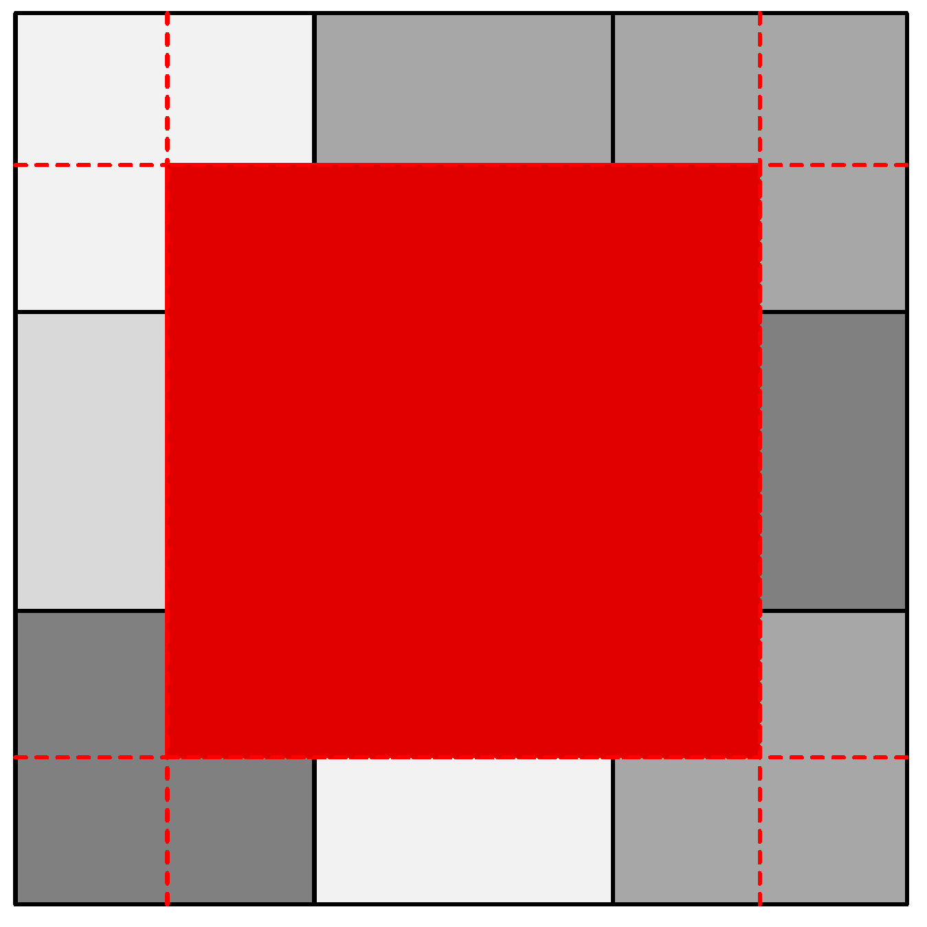
3.2. Reprojection and Resampling of the Downscaled 15-m Data into Registration with the Sentinel-2A 20-m Data

Landsat-8 and Sentinel-2A data are misaligned because their tiling schemes are different and because the Landsat-8 geolocation framework contains residual errors that vary among Landsat path/rows [19]. The pairs of Sentinel-2A and Landsat-8 images (Table 2) were aligned using an automated feature and area-based least squares matching approach that provides sub-pixel precision matching [18]. First the Landsat-8 30-m near infrared (NIR) band was resampled to 20-m resolution and then matched with the Sentinel-2A NIR 20-m band. Then following the recommendations of Yan et al. [18] an affine transformation was used to characterize the spatial relation between the matched sensor data, defined as:

$$\{\begin{array}{l}{x}_L=a_0+a_1{x}_S+a_2{y}_S\\ y_L=b_0+b_1{x}_S+b_2{y}_S\end{array},$$

(3)

where $x_L$, $y_L$ are the UTM coordinates in the Landsat-8 image, $x_S$, $y_S$ are the UTM coordinates in the Sentinel-2A 20-m data, and $a_i$, $b_i$ are the affine transformation coefficients.

Each band of the Landsat-8 15-m data, derived as Equation (2), was reprojected into registration with the Sentinel-2A 20-m grid using the affine transformation coefficients. In this way the Landsat-8 15-m band data were only resampled once. The indirect approach [48] was used whereby the location of each Sentinel-2A 20-m image pixel was reprojected as Equation (3) into the Landsat-8 image and then the Landsat-8 15-m band values were resampled to 20-m resolution. Bilinear and cubic convolution resamplers were considered and for brevity the results are termed as bilinear-based LPAD and cubic convolution-based LPAD results respectively.

4. Evaluation Methodology

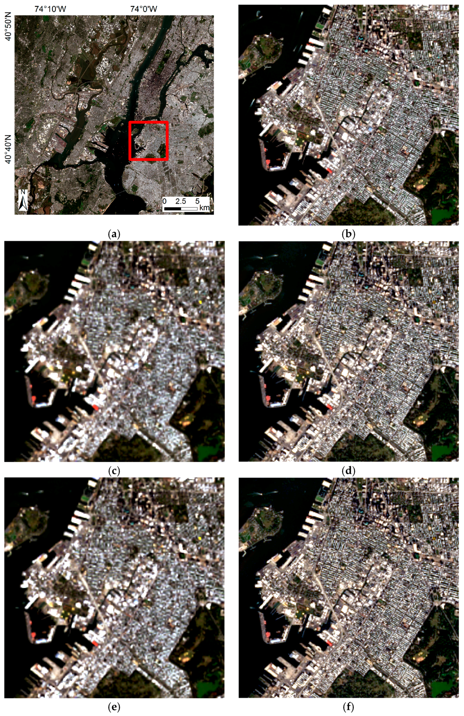
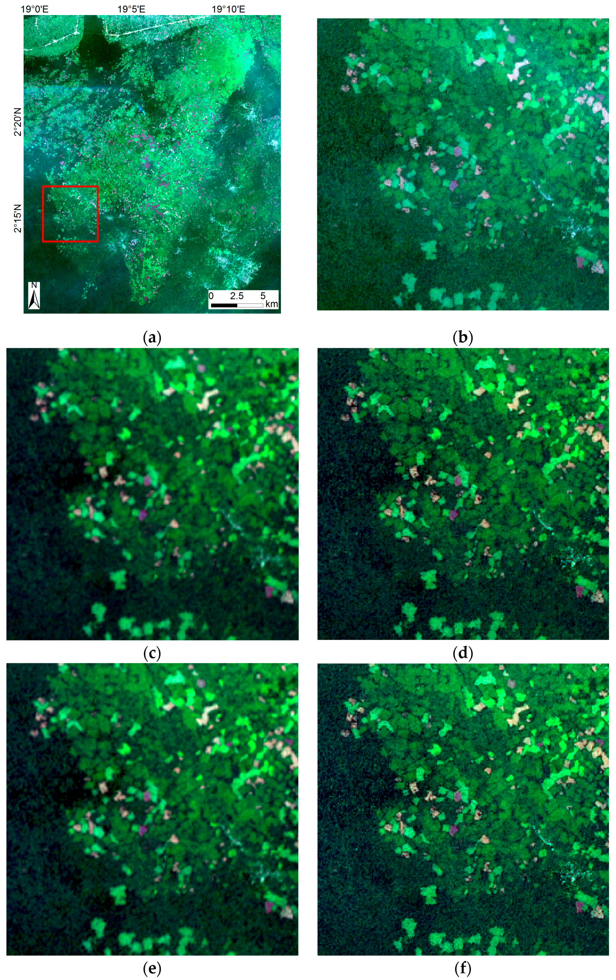
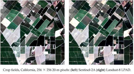
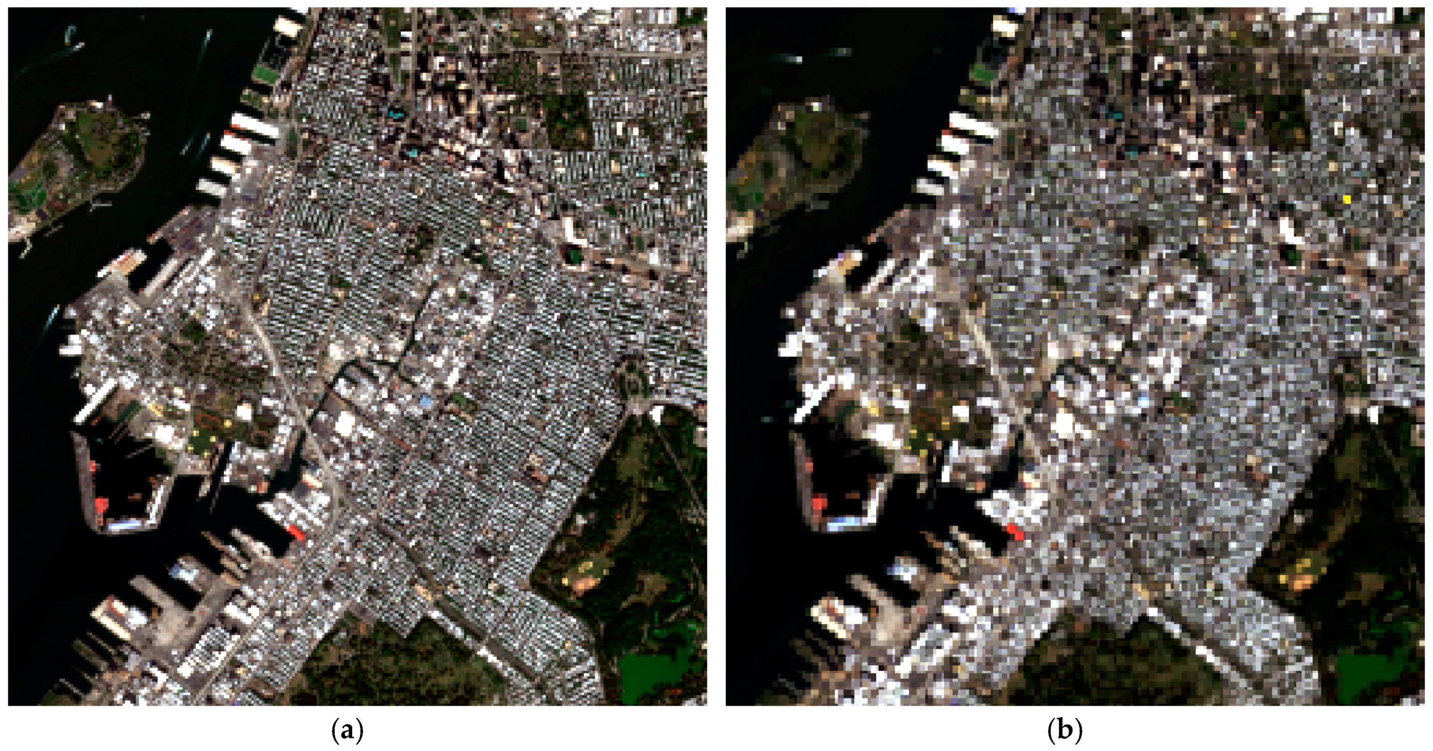
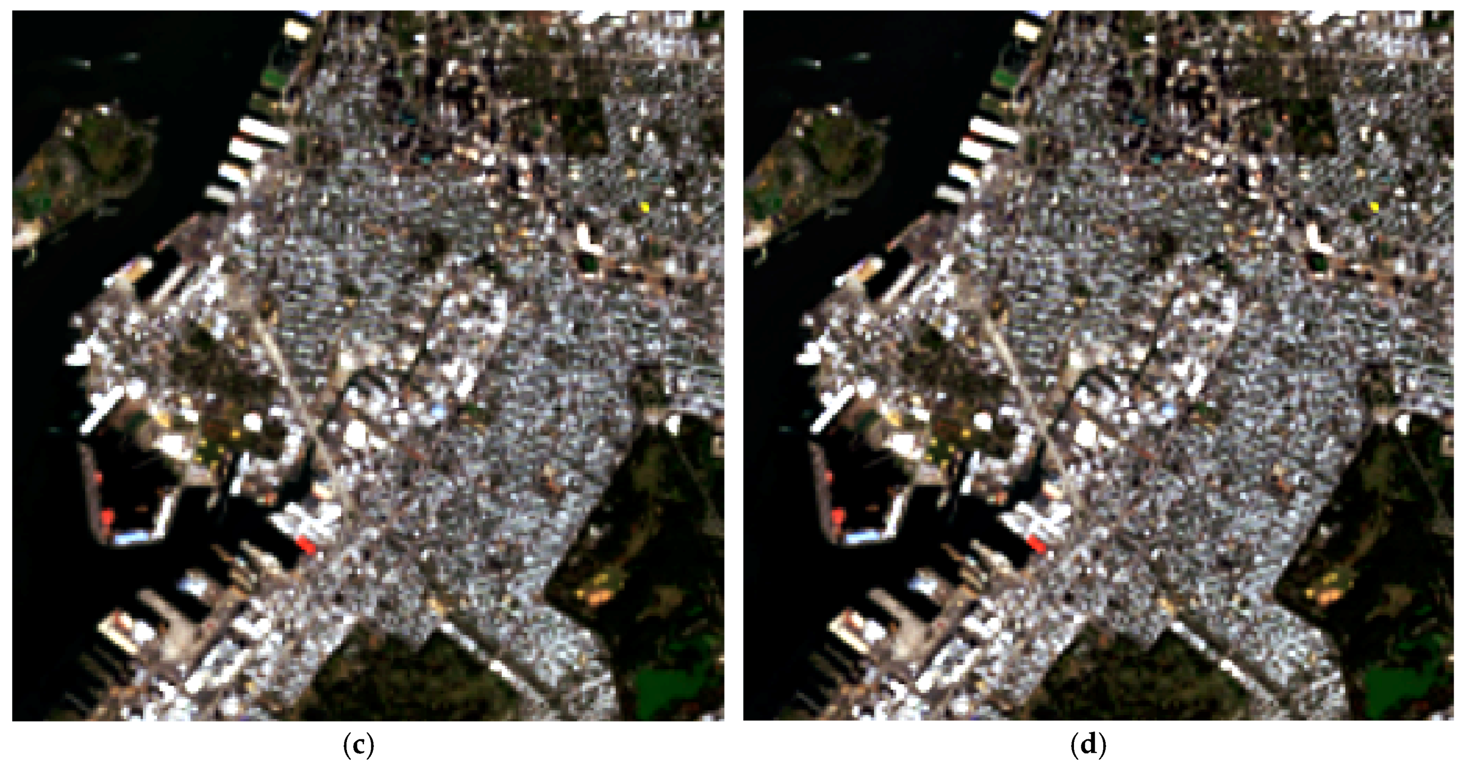
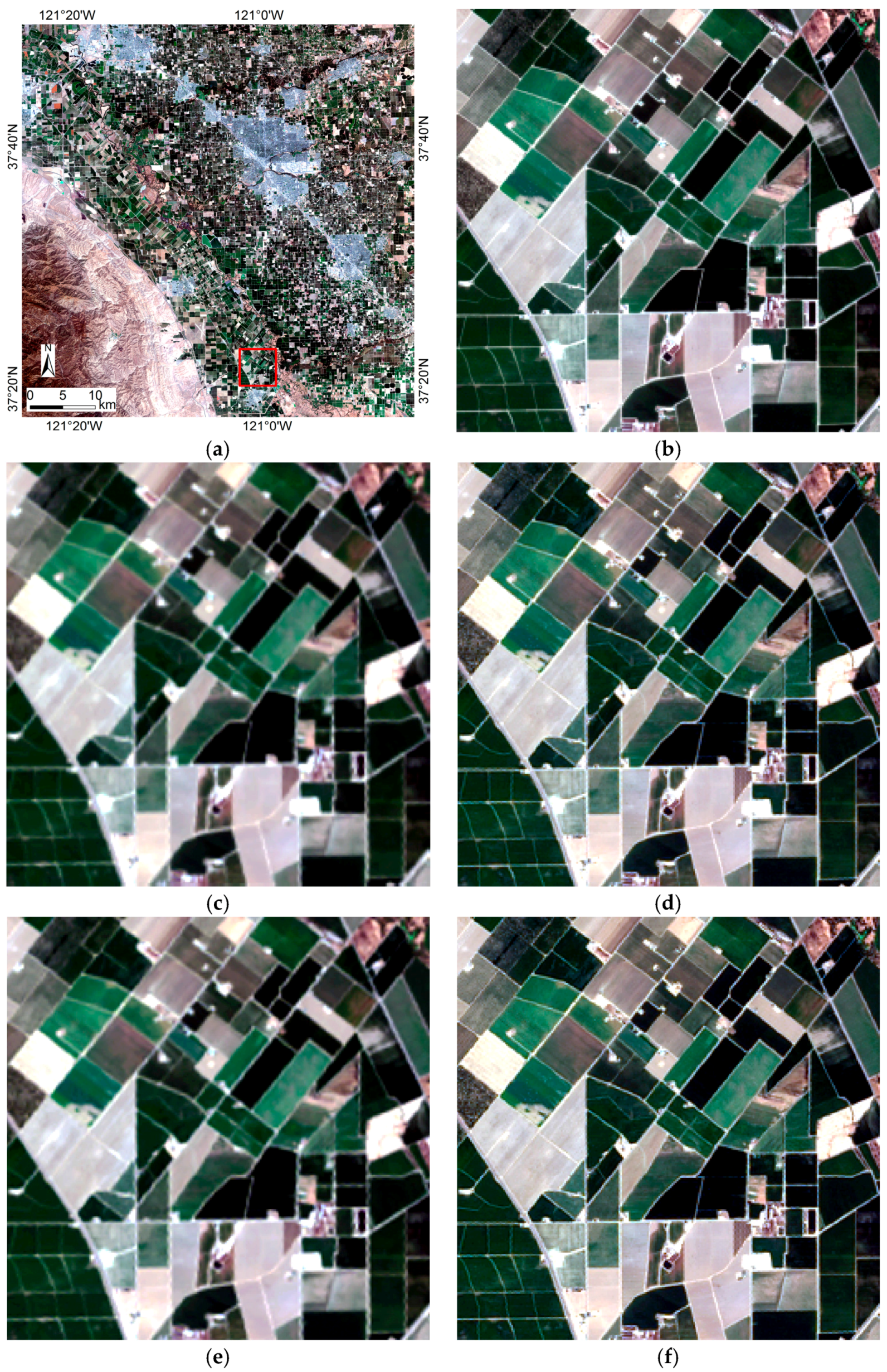
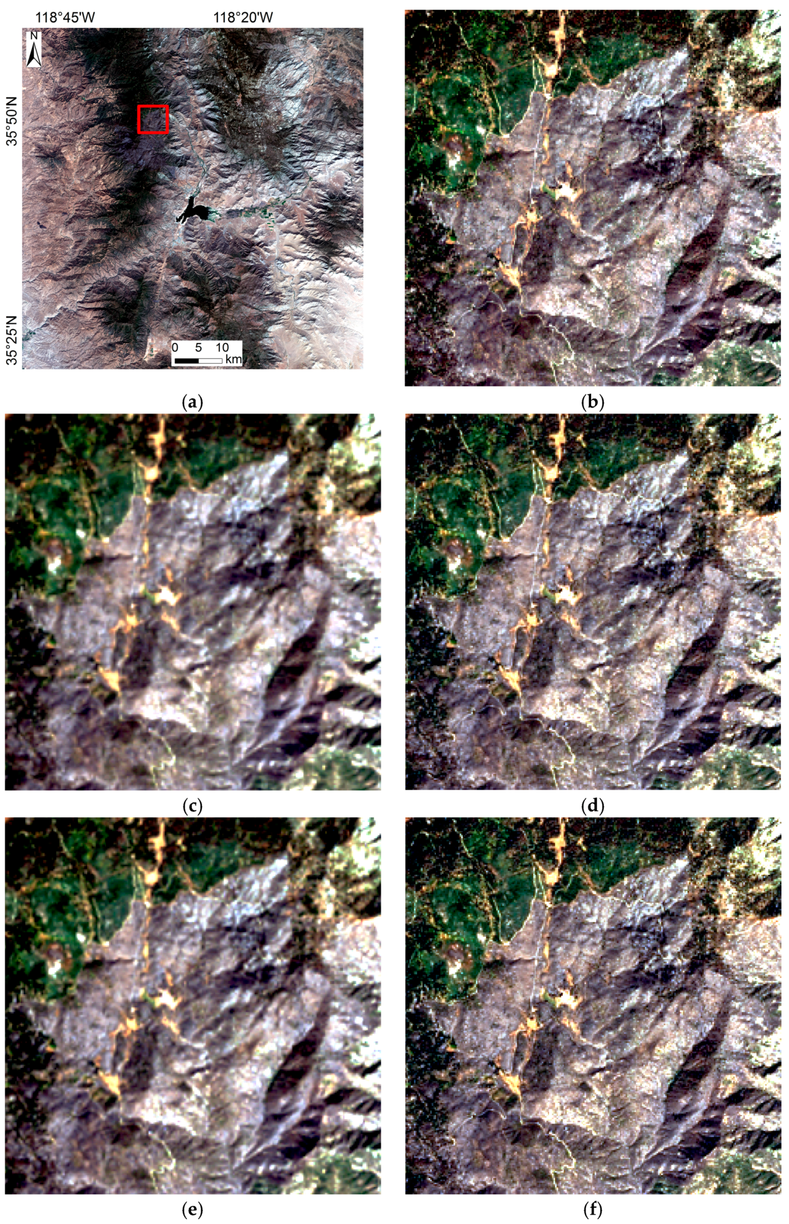
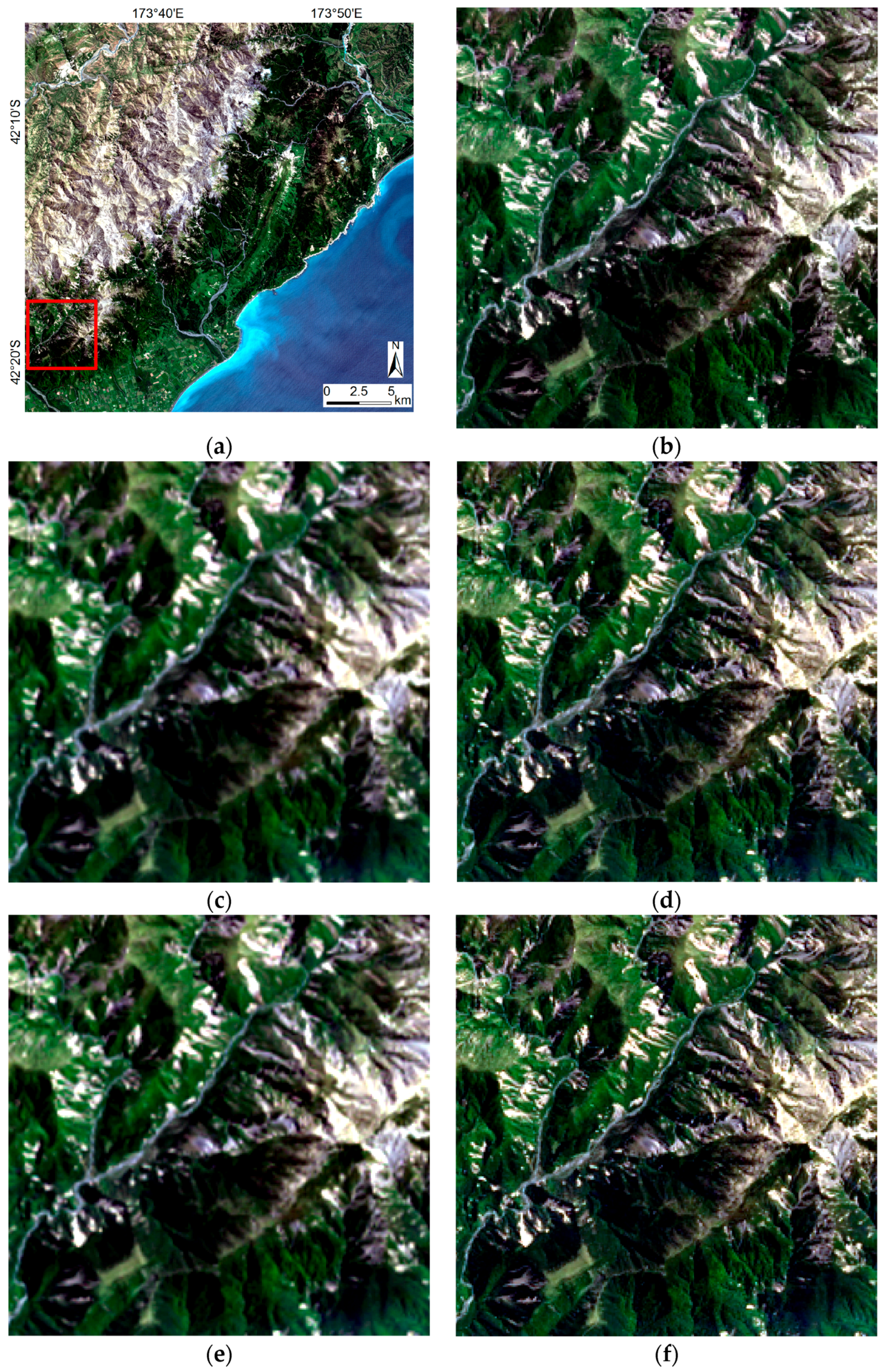
To provide a control data set, Landsat-8 downscaling from 30 m to 20 m was undertaken using conventional resampling, i.e., without the LPAD approach. Nearest neighbor, bilinear and cubic convolution resamplers were considered. The nearest neighbor resampling method selects the closest pixel and so preserves the input data values but is known to create pixel “blockiness” and locational shifts up to $\sqrt{2}/2$ pixels [49]. Bilinear and cubic convolution resamplers smooth the data by interpolating from the 4 and 16 surrounding pixels, respectively [50,51]. Under certain assumptions cubic convolution is theoretically optimal but usually these assumptions are not met and consequently cubic convolution resampled data may have edge-over and under-shoot issues along high contrast edges [52].

The Landsat-8 data downscaled to 20-m resolution using the LPAD method and the control, i.e., conventionally resampled to 20-m Landsat-8 data, were compared with the corresponding Sentinel-2A 20-m data for each site (Table 2). As the Sentinel-2A red, green, and blue bands are defined at 10 m (Table 1) these bands were degraded to 20 m by simple averaging without considering the Sentinel-2A point spread function as it is currently unknown. Note that, unlike for Landsat-8, four adjacent Sentinel-2A 10-m pixels nest within each 20-m pixel, and so averaging is straightforward.

The LPAD and control Landsat-8 20-m data were compared visually and quantitatively with the Sentinel-2A 20-m data. This was undertaken considering the three true color (red, green, and blue) bands and considering all six spectrally similar bands (Table 1). Our expectation is that because the Landsat-8 15-m panchromatic band has a bandwidth that includes only the Landsat-8 red, green, and blue bands the LPAD approach will work better for the true color than for the other bands.

Quantitative comparison of the data was undertaken using the ${Q2}^n$ metric that quantifies the average spatial and spectral distortion between any number of bands between two images [53]. The ${Q2}^n$ metric is a single value bounded between 0 and 1 (where higher values indicate greater quality and less distortion) and is an extension of the single band universal image quality index (UQI) [54]. The UQI is widely used as, similar to human visual perception, it is sensitive to the structural information differences, which is not the case for conventional image difference statistics. In this study the ${Q2}^n$ values were calculated with respect to non-overlapping adjacent n × n pixel windows and then averaged to yield a single image value. The same n = 32 pixel window dimensions used to assess downscaling Landsat-8 30 m to 15 m [46] was implemented.

5. Results

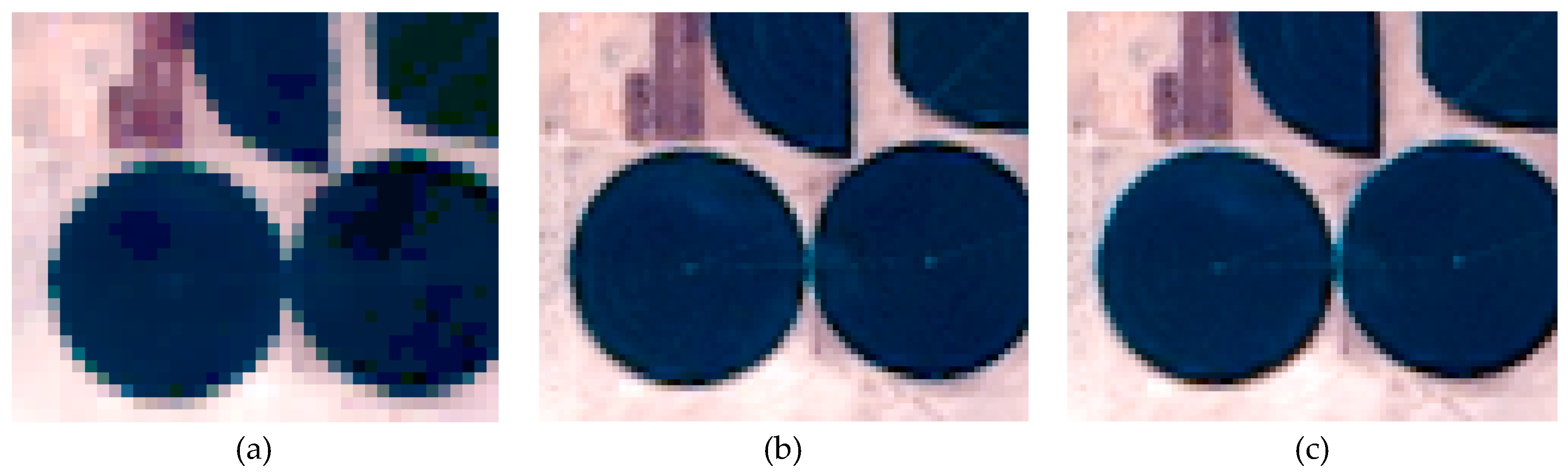
5.1. Conventional Resampling (Nearest Neighbor, Bilinear, and Cubic Convolution) Based Downscaling

Figure 3 illustrates the results of Landsat-8 downscaling from 30 m to 20 m using three conventional resampling approaches. The New York true color image subset is illustrated because it contains high spatial frequency features associated with closely packed city blocks, roads, rivers and parks. Compared to the Sentinel-2A 20-m data (a) the conventionally resampled Landsat-8 data (b), (c), and (d), do not contain the same level of spatial detail. In particular, the nearest-neighbor resampled data (b) are inferior with the aforementioned “blockiness” and locational shifts apparent with much of the detail in the areas of road and buildings quite obviously lost. The bilinear (c) and cubic convolution (d) resampled Landsat-8 data appear very similar and both smooth the spatial detail.

The ${Q2}^n$ values derived by comparing the illustrated 20-m Sentinel-2A image with the nearest neighbor, bilinear, and cubic convolution resampled Landsat-8 20-m images are 0.7142, 0.7520, and 0.7760, respectively. Thus, quantitatively the nearest neighbor and cubic convolution resampled data were the most and least distorted (spectrally and spatially) respectively compared to the Sentinel-2A data. Given the better performance of the bilinear and cubic convolution resamplers, for the remainder of this study they are both considered in the LPAD downscaling, i.e., bilinear-based LPAD and cubic convolution-based LPAD results are presented.

5.2. LPAD Downscaling

Figure 4, Figure 5, Figure 6, Figure 7 and Figure 8 illustrate, for the five sites (Table 2), the Sentinel-2A 20-m true color images (a) and 256 × 256 20-m pixel Sentinel-2A sub-sets selected over regions of high image spatial contrast (b). In addition, for each sub-set, the conventional Landsat-8 bilinear (c) and cubic convolution (e) resampled 20-m data, and the bilinear-based LPAD (d) and cubic convolution-based LPAD (f) 20-m results are illustrated.

It is evident that the LPAD 20-m results provide more clear object boundaries and finer spatial detail than the conventionally resampled 20-m data. Visually, the LPAD generated 20-m data appear spatially and spectrally almost the same as the Sentinel-2A 20-m reference data. The texture of the New York city blocks and even other fine objects can be unambiguously identified (Figure 4d,f). In contrast, the object boundaries are blurry in the 20-m urban areas resampled from the original 30-m data using bilinear and cubic convolution resamplers (Figure 4c,e) and the fine spatial and textural details of the city blocks are degraded. The LPAD generated Landsat-8 20-m crop fields (Figure 5d,f) have sharper boundaries than the Landsat-8 20-m conventionally resampled band data (Figure 5c,e). Similarly, the LPAD generated Landsat-8 20-m burned areas (Figure 6d,f) boundaries appear more distinct than the bilinear and cubic convolution resampling generated 20-m results (Figure 6c,e). The LPAD generated Landsat-8 20-m landslides (Figure 7d,f) appear identical to the Sentinel-2A 20-m reference data (Figure 7b). The small and elongated landslides can be visually identified in LPAD generated 20-m data but they are blurry and cannot be accurately identified in the bilinear and cubic convolution resampled 20-m data (Figure 7c,e). The LPAD generated 20-m deforested patches (Figure 8d,f) appear almost consistent with the Sentinel-2A 20-m reference data (Figure 8b) and their boundaries are more blurred in the bilinear and cubic convolution resampled data (Figure 8c,e). In general, objects with pixel-scale small axis dimensions, such as narrow roads, are visually discernable in the LPAD generated Landsat-8 20-m data but not in the bilinear and cubic convolution resampled 20-m data.

Table 3. ${Q2}^n$ values comparing the Sentinel-2A 20-m data with the conventional bilinear (BL), BL-based LPAD, conventional cubic convolution (CC), and CC-based LPAD Landsat-8 20-m data. Results for the true color reflectance (red, green, blue) bands (Table 1) and the image areas illustrated in Figure 4a, Figure 5a, Figure 6a, Figure 7a and Figure 8a.

Location—Major Land Cover	BL Resampler	BL-Based LPAD	CC Resampler	CC-Based LPAD
New York—urban area	0.7770	0.8970	0.8017	0.8953
California—crop fields	0.8826	0.9294	0.8955	0.9223
California—burned forest	0.9025	0.9608	0.9165	0.9547
New Zealand—landslides	0.7132	0.7511	0.7247	0.7474
Congo—tropical forest	0.7334	0.7330	0.7431	0.7080

and

Table 4. ${Q2}^n$ values comparing the Sentinel-2A 20-m data with the conventional bilinear (BL), BL-based LPAD, conventional cubic convolution (CC), and CC-based LPAD Landsat-8 20-m data. Results for the six corresponding Sentinel-2A and Landsat-8 bands (Table 1) and the image areas are illustrated in Figure 4a, Figure 5a, Figure 6a, Figure 7a and Figure 8a.

Location—Major Land Cover	BL Resampler	BL-Based LPAD	CC Resampler	CC-Based LPAD
New York—urban area	0.8227	0.8870	0.8414	0.8787
California—crop fields	0.9205	0.9410	0.9298	0.9333
California—burned forest	0.9290	0.9590	0.9388	0.9505
New Zealand—landslides	0.7385	0.7569	0.7465	0.7524
Congo—tropical forest	0.7989	0.7955	0.8039	0.7780

summarize quantitative comparisons (i.e., ${Q2}^n$ values, where lower values indicate more distortion) between the Sentinel-2A 20-m data and the various combinations of downscaled data considering the whole image areas illustrated in Figure 4a, Figure 5a, Figure 6a, Figure 7a and Figure 8a.

Table 3 summarizes the results considering just the red, green, and blue bands. For all the sites, except the Congo forest site, the conventional bilinear resampling approach has the most distortion, followed in descending order of distortion by the conventional cubic convolution resampling, cubic convolution-based LPAD, and bilinear-based LPAD approaches. The ${Q2}^n$ differences between the conventional bilinear and cubic-convolution resampling site results are expected for the reasons discussed above (Section 5.1). However, less immediately expected is the higher performance of the bilinear-based LPAD approach compared to the cubic convolution-based LPAD approach.

The Congo forest site results are anomalous compared to the other sites (Table 3). There is negligible difference between the conventional bilinear and bilinear-based LPAD approaches (both have ${Q2}^n$ = 0.733 to 3 d.p), the least distortion is for the conventional cubic convolution resampling approach (0.743), and the cubic convolution-based LPAD approach has the most distortion (0.708). Unlike for the other sites, the Congo Sentinel-2A and Landsat-8 data were acquired one day apart (Table 2) and the atmosphere changed during this period, with aerosol from biomass burning apparent in the Sentinel-2A data with much less apparent aerosols the day before in the Landsat-8 data (Figure 8).

Table 4 summarizes the same results as for Table 3 but considering all six corresponding bands and not just the red, green and blue bands. The same pattern of ${Q2}^n$ values in Table 4 as Table 3 is found. For all the sites, except the Congo forest site, the conventional bilinear resampling approach has the most distortion, followed in descending order of distortion by the conventional cubic convolution resampling, cubic convolution-based LPAD, and then the bilinear-based LPAD approaches.

6. Discussion

The integration of Landsat-8 and Sentinel-2 data for both research and applications is expected to receive growing attention in the global change research community [3,4]. One challenge is the spatial resolution difference between the sensors. Rather than downscaling by conventional resampling, that we showed (Figure 3) will cause either smoothing of the downscaled results (e.g., with convention bilinear or cubic convolution resampling) or introduce locational shifts (e.g., with nearest neighbor resampling or pixel duplication approaches), the Landsat-8 15-m panchromatic band was used to assist the downscaling of the Landsat-8 OLI 30-m bands to 20 m. We note that it is not meaningful to downscale Landsat-8 data to 10 m using the LPAD method as the Landsat-8 panchromatic band is defined at 15 m.

Visual comparisons demonstrated that the LPAD method introduced less spectral and spatial distortion than conventional bilinear and cubic convolution resampling. The bilinear-based LPAD approach performed systematically better than the cubic convolution-based LPAD approach. This was because after downscaling from 30 m to 15 m the Landsat-8 15-m data were resampled to 20 m. This resampling from 15 m to 20 m is more like a pixel aggregation problem than an interpolation problem. In such cases, previous studies have noted the advantage of bilinear over cubic convolution resampling [55,56].

Our expectation was that because the Landsat-8 15-m panchromatic band has a bandwidth that includes only the Landsat-8 red, green and blue bands [46] the LPAD approach would work better for these three OLI bands than for the other bands (Table 1). However, the same pattern of the $Q{2}^n$ values considering just the red, green, and blue bands (Table 3) and considering all six spectral bands (Table 4) was found. Perhaps this reflects the reduced atmospheric scattering that occurs at longer wavelengths [57,58]. The results of this study indicate that the LPAD approach can be applied to downscale all of the Landsat-8 30-m OLI bands.

The Democratic Republic of the Congo results were anomalous, with negligible difference between the $Q{2}^n$ values for the conventional bilinear and bilinear-based LPAD approaches. They were included, not because there is anything particularly different about the Congo scene content compared to the other four sites, but because their results illustrate an important issue. Specifically, atmospheric and perhaps surface differences (due to biomass burning) between the Landsat-8 and Sentinel-2A images meant that differences between the downscaled Landsat-8 20 m and Sentinel-2A 20 m were not due only to the downscaling. The Sentinel-2A image was acquired a day after the Landsat-8 image and contained spatially extensive aerosols that are known to scatter and absorb radiation and that effectively reduce the image contrast [57,58]. Atmospheric correction methodologies that use radiative transfer algorithms and atmospheric characterization data are most suitable for large area and/or repeat atmospheric correction [25]. Unfortunately, to date, there is no publically available Landsat-8 and Sentinel-2A atmospheric correction approach that uses the same radiative transfer algorithm and atmospheric characterization approach. Evidently, fusion of Landsat-8 and Sentinel-2A data should be undertaken with caution when images are acquired at different times [59] unless the data are acquired with similar surface and atmospheric conditions or are pre-processed very robustly.

In this study we did not consider sensor differences due to different viewing geometry conditions combined with surface reflectance anisotropy [15,16], or sensor spectral band pass differences [60,61], or differences in the interaction of radiation with the atmosphere across high contrast edges (“adjacency effects”) that are dependent on the atmospheric contents and the sensor point spread function [62,63]. These sensor differences are scene dependent and are likely to cause systematic distortions between the Sentinel-2A and Landsat-8 data. Despite this, with the exception of the Congo results, the bilinear-based LPAD approach provided the best downscaling results with less spatial and spectral distortion than conventional resampling approaches.

In the LPAD method the Landsat-8 30-m band data are first downscaled to 15 m using the simple Brovey method [45] with fixed spectral weights derived by considering a large number of laboratory spectra and the Landsat-8 OLI spectral response functions [46]. This is computationally efficient and so is appropriate for global application. Computation efficiency is important for large-area or long-term Landsat-8 and Sentinel-2 studies due to the high satellite data volumes. However, for small data volumes, and/or when computational constraints are not an issue [64], advanced downscaling methods [41] could be used to provide less spatial and spectral distortion, although such improvements are usually subtle and less than the noise introduced by atmospheric and sun-sensor-target geometry effects [46].

7. Conclusions

A new way to downscale Landsat-8 30-m OLI data to Sentinel-2 20-m resolution was presented. Rather than downscale by conventional resampling, that will cause either smoothing of the downscaled results or introduce pixel-level locational shifts, the Landsat-8 15-m panchromatic band is used to assist the Landsat-8 30-m downscaling. The Landsat panchromatic-assisted downscaling (LPAD) approach was tested over five study areas with different land covers and containing anthropogenic and natural features with straight and irregular boundaries. Near-contemporaneous Sentinel-2A 20-m data were used as reference data for qualitative and quantitative comparison. Results demonstrated that (1) the LPAD method introduced less spectral and spatial distortion and provided visually more coherent data than traditional bilinear and cubic convolution resampling approaches; (2) the LPAD approach can be effectively applied to downscaling the Landsat-8 30-m OLI bands; (3) the bilinear-based LPAD approach provided the least spectral and spatial distortion; and (4) Landsat-8 and Sentinel-2A data fusion should be undertaken with caution when images are acquired at different times under different atmospheric conditions. The LPAD source code is made available at GitHub for public use and evaluation at https://github.com/jasonleepolyu/Landsat-Panchromatic-Assisted-Downscaling-LPAD-/tree/master.

References

1. Irons, J.R.; Dwyer, J.L.; Barsi, J.A. The next Landsat satellite: The Landsat data continuity mission. Remote Sens. Environ. 2012, 122, 11–21. [Google Scholar] [CrossRef]
2. Drusch, M.; Del Bello, U.; Carlier, S.; Colin, O.; Fernandez, V.; Gascon, F.; Hoersch, B.; Isola, C.; Laberinti, P.; Martimort, P.; et al. Sentinel-2: ESA’s optical high-resolution mission for GMES operational services. Remote Sens. Environ. 2012, 120, 25–36. [Google Scholar] [CrossRef]
3. Roy, D.P.; Wulder, M.A.; Loveland, T.R.; Woodcock, C.E.; Allen, R.G.; Anderson, M.C.; Helder, D.; Irons, J.R.; Johnson, D.M.; Kennedy, R.; et al. Landsat-8: Science and product vision for terrestrial global change research. Remote Sens. Environ. 2014, 145, 154–172. [Google Scholar] [CrossRef]
4. Malenovský, Z.; Rott, H.; Cihlar, J.; Schaepman, M.E.; García-Santos, G.; Fernandes, R.; Berger, M. Sentinels for science: Potential of Sentinel-1, -2, and -3 missions for scientific observations of ocean, cryosphere, and land. Remote Sens. Environ. 2012, 120, 91–101. [Google Scholar] [CrossRef]
5. Whitcraft, A.K.; Becker-Reshef, I.; Killough, B.D.; Justice, C.O. Meeting earth observation requirements for global agricultural monitoring: An evaluation of the revisit capabilities of current and planned moderate resolution optical earth observing missions. Remote Sens. 2015, 7, 1482–1503. [Google Scholar] [CrossRef]
6. Inglada, J.; Arias, M.; Tardy, B.; Hagolle, O.; Valero, S.; Morin, D.; Dedieu, G.; Sepulcre, G.; Bontemps, S.; Defourny, P.; et al. Assessment of an operational system for crop type map production using high temporal and spatial resolution satellite optical imagery. Remote Sens. 2015, 7, 12356–12379. [Google Scholar] [CrossRef]
7. Bontemps, S.; Arias, M.; Cara, C.; Dedieu, G.; Guzzonato, E.; Hagolle, O.; Inglada, J.; Matton, N.; Morin, D.; Popescu, R.; et al. Building a data set over 12 globally distributed sites to support the development of agriculture monitoring applications with Sentinel-2. Remote Sens. 2015, 7, 16062–16090. [Google Scholar] [CrossRef]
8. Wulder, M.A.; Hilker, T.; White, J.C.; Coops, N.C.; Masek, J.G.; Pflugmacher, D.; Crevier, Y. Virtual constellations for global terrestrial monitoring. Remote Sens. Environ. 2015, 170, 62–76. [Google Scholar] [CrossRef]
9. Paul, F.; Winsvold, S.H.; Kääb, A.; Nagler, T.; Schwaizer, G. Glacier remote sensing using Sentinel-2. Part II: Mapping glacier extents and surface facies, and comparison to Landsat 8. Remote Sens. 2016, 8, 575. [Google Scholar] [CrossRef]
10. Markham, B.; Barsi, J.; Kvaran, G.; Ong, L.; Kaita, E.; Biggar, S.; Czapla-Myers, J.; Mishra, N.; Helder, D. Landsat-8 operational land imager radiometric calibration and stability. Remote Sens. 2014, 6, 12275–12308. [Google Scholar] [CrossRef]
11. Morfitt, R.; Barsi, J.; Levy, R.; Markham, B.; Micijevic, E.; Ong, L.; Scaramuzza, P.; Vanderwerff, K. Landsat-8 Operational Land Imager (OLI) radiometric performance on-orbit. Remote Sens. 2015, 7, 2208–2237. [Google Scholar] [CrossRef]
12. Gascon, F.; Bouzinac, C.; Thépaut, O.; Jung, M.; Francesconi, B.; Louis, J.; Lonjou, V.; Lafrance, B.; Massera, S.; Gaudel-Vacaresse, A.; et al. Copernicus Sentinel-2 calibration and products validation status. Remote Sens. 2017, 9, 584. [Google Scholar] [CrossRef]
13. Vermote, E.; Justice, C.; Claverie, M.; Franch, B. Preliminary analysis of the performance of the Landsat 8/OLI land surface reflectance product. Remote Sens. Environ. 2016, 185, 46–56. [Google Scholar] [CrossRef]
14. Hagolle, O.; Huc, M.; Villa Pascual, D.; Dedieu, G. A multi-temporal and multi-spectral method to estimate aerosol optical thickness over land, for the atmospheric correction of FormoSat-2, Landsat, VENμS and Sentinel-2 images. Remote Sens. 2015, 7, 2668–2691. [Google Scholar] [CrossRef]
15. Roy, D.P.; Zhang, H.K.; Ju, J.; Gomez-Dans, J.L.; Lewis, P.E.; Schaaf, C.B.; Sun, Q.; Li, J.; Huang, H.; Kovalskyy, V. A general method to normalize Landsat reflectance data to nadir BRDF adjusted reflectance. Remote Sens. Environ. 2016, 176, 255–271. [Google Scholar] [CrossRef]
16. Roy, D.P.; Li, J.; Zhang, H.K.; Yan, L.; Huang, H.; Li, Z. Examination of Sentinel-2A multi-1 spectral instrument (MSI) reflectance anisotropy and the suitability of a general method to normalize MSI reflectance to nadir BRDF adjusted reflectance. Remote Sens. Environ. 2017, 199, 25–38. [Google Scholar] [CrossRef]
17. Roy, D.P.; Li, J.; Zhang, H.K.; Yan, L. Best practices for the reprojection and resampling of Sentinel-2 Multi Spectral Instrument Level 1C data. Remote Sens. Lett. 2016, 7, 1023–1032. [Google Scholar] [CrossRef]
18. Yan, L.; Roy, D.P.; Zhang, H.; Li, J.; Huang, H. An automated approach for sub-pixel registration of Landsat-8 Operational Land Imager (OLI) and Sentinel-2 Multi Spectral Instrument (MSI) imagery. Remote Sens. 2016, 8, 520. [Google Scholar] [CrossRef]
19. Storey, J.; Roy, D.P.; Masek, J.; Gascon, F.; Dwyer, J.; Choate, M. A note on the temporary misregistration of Landsat-8 Operational Land Imager (OLI) and Sentinel-2 Multi Spectral Instrument (MSI) imagery. Remote Sens. Environ. 2016, 186, 121–122. [Google Scholar] [CrossRef]
20. Mandanici, E.; Bitelli, G. Preliminary comparison of Sentinel-2 and Landsat 8 Imagery for a combined use. Remote Sens. 2016, 8, 1014. [Google Scholar] [CrossRef]
21. Skakun, S.; Roger, J.C.; Vermote, E.F.; Masek, J.G.; Justice, C.O. Automatic sub-pixel co-registration of Landsat-8 Operational Land Imager and Sentinel-2A Multi-Spectral Instrument images using phase correlation and machine learning based mapping. Int. J. Digit. Earth. 2017, 23, 1–17. [Google Scholar] [CrossRef]
22. Pelletier, C.; Valero, S.; Inglada, J.; Champion, N.; Dedieu, G. Assessing the robustness of Random Forests to map land cover with high resolution satellite image time series over large areas. Remote Sens. Environ. 2016, 187, 156–168. [Google Scholar] [CrossRef]
23. Loveland, T.R.; Irons, J.R. Landsat 8: The plans, the reality, and the legacy. Remote Sens. Environ. 2016, 185, 1–6. [Google Scholar] [CrossRef]
24. Montanaro, M.; Gerace, A.; Lunsford, A.; Reuter, D. Stray light artifacts in imagery from the Landsat 8 Thermal Infrared Sensor. Remote Sens. 2014, 6, 10435–10456. [Google Scholar] [CrossRef]
25. Ju, J.; Roy, D.P.; Vermote, E.; Masek, J.; Kovalskyy, V. Continental-scale validation of MODIS-based and LEDAPS Landsat ETM+ atmospheric correction methods. Remote Sens. Environ. 2012, 122, 175–184. [Google Scholar] [CrossRef]
26. Storey, J.; Choate, M.; Lee, K. Landsat 8 Operational Land Imager on-orbit geometric calibration and performance. Remote Sens. 2014, 6, 11127–11152. [Google Scholar] [CrossRef]
27. Loveland, T.R.; Dwyer, J.L. Landsat: Building a strong future. Remote Sens. Environ. 2012, 122, 22–29. [Google Scholar] [CrossRef]
28. European Space Agency (ESA). Sentinel-2 User Handbook; Issue 1, Revision 2; European Space Agency (ESA): Paris, France, 2015. [Google Scholar]
29. Languille, F.; Déchoz, C.; Gaudel, A.; Greslou, D.; De Lussy, F.; Trémas, T.; Poulain, V. Sentinel-2 geometric image quality commissioning: First results. Proc. SPIE 2015. [Google Scholar] [CrossRef]
30. Anderson, M.C.; Norman, J.M.; Mecikalski, J.R.; Torn, R.D.; Kustas, W.P.; Basara, J.B. A multiscale remote sensing model for disaggregating regional fluxes to micrometeorological scales. J. Hydrometeorol. 2004, 5, 343–363. [Google Scholar] [CrossRef]
31. Pouteau, R.; Rambal, S.; Ratte, J.P.; Gogé, F.; Joffre, R.; Winkel, T. Downscaling MODIS-derived maps using GIS and boosted regression trees: The case of frost occurrence over the arid Andean highlands of Bolivia. Remote Sens. Environ. 2011, 115, 117–129. [Google Scholar] [CrossRef]
32. Zhang, H.; Huang, B. Support vector regression-based downscaling for intercalibration of multiresolution satellite images. IEEE Trans. Geosci. Remote Sens. 2013, 51, 1114–1123. [Google Scholar] [CrossRef]
33. Duveiller, G.; Cescatti, A. Spatially downscaling sun-induced chlorophyll fluorescence leads to an improved temporal correlation with gross primary productivity. Remote Sens. Environ. 2016, 182, 72–89. [Google Scholar] [CrossRef]
34. Che, X.; Yang, Y.; Feng, M.; Xiao, T.; Huang, S.; Xiang, Y.; Chen, Z. Mapping extent dynamics of small lakes using downscaling MODIS surface reflectance. Remote Sens. 2017, 9, 82. [Google Scholar] [CrossRef]
35. Zhang, Y.; Backer, S.D.; Scheunders, P. Noise-resistant wavelet-based Bayesian fusion of multispectral and hyperspectral images. IEEE Trans. Geosci. Remote Sens. 2009, 47, 3834–3843. [Google Scholar] [CrossRef]
36. Garzelli, A. A review of image fusion algorithms based on the super-resolution paradigm. Remote Sens. 2016, 8, 797. [Google Scholar] [CrossRef]
37. Yang, Y.; Anderson, M.C.; Gao, F.; Hain, C.R.; Semmens, K.A.; Kustas, W.P.; Noormets, A.; Wynne, R.H.; Thomas, V.A.; Sun, G. Daily Landsat-scale evapotranspiration estimation over a forested landscape in North Carolina, USA, using multi-satellite data fusion. Hydrol. Earth Syst. Sci. 2017, 21, 1017–1037. [Google Scholar] [CrossRef]
38. Gao, F.; Anderson, M.C.; Zhang, X.; Yang, Z.; Alfieri, J.G.; Kustas, W.P.; Mueller, R.; Johnson, D.M.; Prueger, J.H. Toward mapping crop progress at field scales through fusion of Landsat and MODIS imagery. Remote Sens. Environ. 2017, 188, 9–25. [Google Scholar] [CrossRef]
39. Zhu, X.; Helmer, E.H.; Gao, F.; Liu, D.; Chen, J.; Lefsky, M.A. A flexible spatiotemporal method for fusing satellite images with different resolutions. Remote Sens. Environ. 2016, 172, 165–177. [Google Scholar] [CrossRef]
40. Thomas, C.; Ranchin, T.; Wald, L.; Chanussot, J. Synthesis of multispectral images to high spatial resolution: A critical review of fusion methods based on remote sensing physics. IEEE Trans. Geosci. Remote Sens. 2008, 46, 1301–1312. [Google Scholar] [CrossRef] [Green Version]
41. Vivone, G.; Alparone, L.; Chanussot, J.; Dalla Mura, M.; Garzelli, A.; Licciardi, G.A.; Restaino, R.; Wald, L. A critical comparison among pansharpening algorithms. IEEE Trans. Geosci. Remote Sens. 2015, 53, 2565–2586. [Google Scholar] [CrossRef]
42. Alparone, L.; Aiazzi, B.; Baronti, S.; Garzelli, A. Remote Sensing Image Fusion; CRC Press: Boca Raton, FL, USA, 2015. [Google Scholar]
43. Pohl, C.; Van Genderen, J.L. Review article multisensor image fusion in remote sensing: Concepts, methods and applications. Int. J. Remote Sens. 1998, 19, 823–854. [Google Scholar] [CrossRef]
44. Zhang, H.K.; Huang, B. A new look at image fusion methods from a Bayesian perspective. Remote Sens. 2015, 7, 6828–6861. [Google Scholar] [CrossRef]
45. Gillespie, A.R.; Kahle, A.B.; Walker, R.E. Color enhancement of highly correlated images. II. Channel ratio and “chromaticity” transformation techniques. Remote Sens. Environ. 1987, 22, 343–365. [Google Scholar] [CrossRef]
46. Zhang, H.K.; Roy, D.P. Computationally inexpensive Landsat 8 operational land imager (OLI) pansharpening. Remote Sens. 2016, 8, 180. [Google Scholar] [CrossRef]
47. Aiazzi, B.; Baronti, S.; Selva, M.; Alparone, L. Bi-cubic interpolation for shift-free pan-sharpening. ISPRS J. Photogramm. Remote Sens. 2013, 86, 65–76. [Google Scholar] [CrossRef]
48. Roy, D.P.; Ju, J.; Kline, K.; Scaramuzza, P.L.; Kovalskyy, V.; Hansen, M.; Loveland, T.R.; Vermote, E.; Zhang, C. Web-enabled Landsat Data (WELD): Landsat ETM+ composited mosaics of the conterminous United States. Remote Sens. Environ. 2010, 114, 35–49. [Google Scholar] [CrossRef]
49. Dikshit, O.; Roy, D.P. An empirical investigation of image resampling effects upon the spectral and textural supervised classification of a high spatial resolution multispectral image. Photogramm. Eng. Remote Sens. 1996, 62, 1085–1092. [Google Scholar]
50. Shlien, S. Geometric correction, registration, and resampling of Landsat imagery. Can. J. Remote Sens. 1979, 5, 74–89. [Google Scholar] [CrossRef]
51. Park, S.K.; Schowengerdt, R.A. Image reconstruction by parametric cubic convolution. Comput. Vis. Graph. Image Process. 1983, 23, 258–272. [Google Scholar] [CrossRef]
52. Keys, R. Cubic convolution interpolation for digital image processing. IEEE Trans. Acoust. Speech Signal Process. 1981, 29, 1153–1160. [Google Scholar] [CrossRef]
53. Garzelli, A.; Nencini, F. Hypercomplex quality assessment of multi/hyperspectral images. IEEE Geosci. Remote Sens. Lett. 2009, 6, 662–665. [Google Scholar] [CrossRef]
54. Wang, Z.; Bovik, A.C.; Sheikh, H.R.; Simoncelli, E.P. Image quality assessment: From error visibility to structural similarity. IEEE Trans. Image Process. 2004, 13, 600–612. [Google Scholar] [CrossRef]
55. Sridhar, V. Evapotranspiration estimation and scaling effects over the Nebraska Sandhills. Great Plains Res. 2007, 17, 35–45. [Google Scholar]
56. Ershadi, A.; McCabe, M.F.; Evans, J.P.; Walker, J.P. Effects of spatial aggregation on the multi-scale estimation of evapotranspiration. Remote Sens. Environ. 2013, 131, 51–62. [Google Scholar] [CrossRef]
57. Dubovik, O.; Holben, B.; Eck, T.F.; Smirnov, A.; Kaufman, Y.J.; King, M.D.; Tanré, D.; Slutsker, I. Variability of absorption and optical properties of key aerosol types observed in worldwide locations. J. Atmos. Sci. 2002, 59, 590–608. [Google Scholar] [CrossRef]
58. Roy, D.P.; Qin, Y.; Kovalskyy, V.; Vermote, E.F.; Ju, J.; Egorov, A.; Hansen, M.C.; Kommareddy, I.; Yan, L. Conterminous United States demonstration and characterization of MODIS-based Landsat ETM+ atmospheric correction. Remote Sens. Environ. 2014, 140, 433–449. [Google Scholar] [CrossRef]
59. Wang, Q.; Blackburn, G.A.; Onojeghuo, A.O.; Dash, J.; Zhou, L.; Zhang, Y.; Atkinson, P.M. Fusion of Landsat 8 OLI and Sentinel-2 MSI Data. IEEE Trans. Geosci. Remote Sens. 2017, 55, 3885–3899. [Google Scholar] [CrossRef]
60. Steven, M.D.; Malthus, T.J.; Baret, F.; Xu, H.; Chopping, M.J. Intercalibration of vegetation indices from different sensor systems. Remote Sens. Environ. 2003, 88, 412–422. [Google Scholar] [CrossRef]
61. Roy, D.P.; Kovalskyy, V.; Zhang, H.K.; Vermote, E.F.; Yan, L.; Kumar, S.S.; Egorov, A. Characterization of Landsat-7 to Landsat-8 reflective wavelength and normalized difference vegetation index continuity. Remote Sens. Environ. 2016, 185, 57–70. [Google Scholar]
62. Liang, S.; Fang, H.; Chen, M. Atmospheric correction of Landsat ETM+ land surface imagery. I. Methods. IEEE Trans. Geosci. Remote Sens. 2001, 39, 2490–2498. [Google Scholar] [CrossRef]
63. Houborg, R.; McCabe, M.F. Impacts of dust aerosol and adjacency effects on the accuracy of Landsat 8 and RapidEye surface reflectances. Remote Sens. Environ. 2017, 194, 127–145. [Google Scholar] [CrossRef]
64. Yang, J.; Zhang, J.; Huang, G. A parallel computing paradigm for pan-sharpening algorithms of remotely sensed images on a multi-core computer. Remote Sens. 2014, 6, 6039–6063. [Google Scholar] [CrossRef]
Figure 1. Illustration of the 7.5 m row and column shifts that occur between the 15-m panchromatic (gray) and the 30-m reflective band (red) Landsat-8 pixels.
Remotesensing 09 00755 g001
Figure 2. 40 × 33 Landsat-8 30-m image (a) LPAD downscaled to 15-m data (80 × 66) with (b) and without (c) considering the 15-m to 30-m Landsat-8 pixel grid shifts. The Landsat-8 image was acquired 6 November 2016 over a commercial crop field in California (centered on 34.8973°N 117.1505°W) with scene center solar zenith and azimuth of 36.5972° and 159.4612°, respectively.
Remotesensing 09 00755 g002
Figure 3. New York 256 × 256 20-m pixel true color subsets: (a) Sentinel-2A 20-m red, green, blue bands aggregated from the original Sentinel-2A 10-m bands; (b) Landsat-8 20-m red, green, blue bands nearest neighbor resampled from 30 m; (c) Landsat-8 20-m red, green, blue bands bilinear resampled from 30 m; and (d) Landsat-8 20-m red, green, blue bands cubic convolution resampled from 30 m.
Remotesensing 09 00755 g003aRemotesensing 09 00755 g003b
Figure 4. New York city true color images showing: (a) Sentinel-2A 20-m image (1500 × 1500 20-m pixels) and sub-set (red box); (b) Sentinel-2A 256 × 256 20-m pixel sub-set; (c) Landsat-8 bilinear resampled to 20 m; (d) Landsat-8 bilinear-based LPAD 20-m data; (e) Landsat-8 cubic convolution resampled to 20 m; (f) Landsat-8 cubic convolution-based LPAD 20-m data.
Remotesensing 09 00755 g004
Figure 5. Crop field, California, true color images showing: (a) Sentinel-2A 20-m image (3000 × 3000 20-m pixels) and sub-set (red box); (b) Sentinel-2A 256 × 256 20-m pixel sub-set; (c) Landsat-8 bilinear resampled to 20 m; (d) Landsat-8 bilinear-based LPAD 20-m data; (e) Landsat-8 cubic convolution resampled to 20 m; (f) Landsat-8 cubic convolution-based LPAD 20-m data.
Remotesensing 09 00755 g005
Figure 6. Burned forest area, California, true color images showing: (a) Sentinel-2A 20-m image (3600 × 3600 20-m pixels) and sub-set (red box); (b) Sentinel-2A 256 × 256 20-m pixel sub-set; (c) Landsat-8 bilinear resampled to 20 m; (d) Landsat-8 bilinear-based LPAD 20-m data; (e) Landsat-8 cubic convolution resampled to 20 m; (f) Landsat-8 cubic convolution-based LPAD 20-m data.
Remotesensing 09 00755 g006
Figure 7. Mountain landslides, New Zealand, true color images showing: (a) Sentinel-2A 20-m image (1500 × 1500 20-m pixels) and sub-set (red box); (b) Sentinel-2A 256 × 256 20-m pixel sub-area; (c) Landsat-8 bilinear resampled to 20 m; (d) Landsat-8 bilinear-based LPAD 20-m data; (e) Landsat-8 cubic convolution resampled to 20 m; (f) Landsat-8 cubic convolution-based LPAD 20-m data.
Remotesensing 09 00755 g007
Figure 8. Tropical forest, Democratic Republic of the Congo, true color images showing: (a) Sentinel-2A 20-m image (1230 × 1425 20-m pixels) and sub-set (red box); (b) Sentinel-2A 256 × 256 20-m pixel sub-set; (c) Landsat-8 bilinear resampled to 20 m; (d) Landsat-8 bilinear-based LPAD 20-m data; (e) Landsat-8 cubic convolution resampled to 20 m; (f) Landsat-8 cubic convolution-based LPAD 20-m data. The smoke aerosols present in the Sentinel-2A image are evident in the north and west of (a).
Remotesensing 09 00755 g008