Saturation Correction for Nighttime Lights Data Based on the Relative NDVI


1
Key Laboratory for Urban Habitat Environmental Science and Technology, Shenzhen Graduate School, Peking University, Shenzhen 518055, China
2
Department of Urban Planning and Design, The University of Hong Kong, Hong Kong, China
3
Shenzhen Institute of Research and Innovation, The University of Hong Kong, Shenzhen 518075, China
4
Key Laboratory for Earth Surface Processes, Ministry of Education, College of Urban and Environmental Sciences, Peking University, Beijing 100871, China
*
Author to whom correspondence should be addressed.
Remote Sens. 2017, 9(7), 759; https://doi.org/10.3390/rs9070759
Submission received: 3 June 2017
/
Revised: 8 July 2017
/
Accepted: 21 July 2017
/
Published: 22 July 2017
Abstract
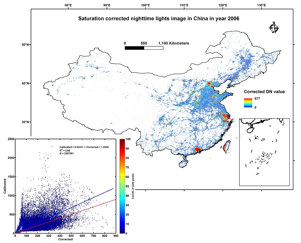
:DMSP/OLS images are widely used as data sources in various domains of study. However, these images have some deficiencies, one of which is digital number (DN) saturation in urban areas, which leads to significant underestimation of light intensity. We propose a new method to correct the saturation. With China as the study area, the threshold value of the saturation DN is screened out first. A series of regression analyses are then carried out for the 2006 radiance calibrated nighttime lights (RCNL) image and relative NDVI (RNDVI) to determine a formula for saturation correction. The 2006 stable nighttime lights (SNL) image (F162006) is finally corrected and evaluated. It is concluded that pixels are saturated when the DN is larger than 50, and that the saturation is more serious when the DN is larger. RNDVI, which was derived by subtracting the interpolated NDVI from the real NDVI, is significantly better than the real NDVI for reflecting the degree of human activity. Quadratic functions describe the relationship between DN and RNDVI well. The 2006 SNL image presented more variation within urban cores and stronger correlations with the 2006 RCNL image and Gross Domestic Product after correction. However, RNDVI may also suffer “saturation” when it is lower than −0.4, at which point it is no longer effective at correcting DN saturation. In general, RNDVI is effective, although far from perfect, for saturation correction of the 2006 SNL image, and could be applied to the SNL images for other years.

1. Introduction
Nighttime lights data obtained by the Operational Linescan System (OLS) on board Defense Meteorological Satellite Program (DMSP) satellites was discovered to have a high correlation with urban characteristics such as Gross Domestic Product (GDP), power assumption, and population levels in the late 20th century [1]. Since then, many more studies in a wide range of disciplines have been conducted to determine useful indicators of human activities [2,3,4,5,6,7,8,9,10,11,12]. The National Aeronautics and Space Administration (NASA) and the National Oceanic and Atmospheric Administration (NOAA) launched the Suomi National Polar Partnership (Suomi-NPP) satellite carrying the first visible infrared imaging radiometer suite (VIIRS) instrument in 2011 and the VIIRS has several improvements over the OLS [13]. Because the VIIRS record began in 2011, any studies prior to that date must rely on DMSP/OLS for nighttime lights imagery. Thus, the importance of the OLS dataset has not decreased.
Scientists at NOAA’s National Geophysical Data Center (NGDC) are in charge of processing the nighttime lights data. They remove natural noises, including moonlight disturbances, aurora light displays, and forest fires, leaving mostly man-made light. They then produce a satellite-year dataset: data from all orbits of a given satellite in a given year are averaged over all valid nights. These datasets, in combination known as the World Stable Lights dataset [14], include data from 1992 to 2013 and are distributed to the public. It has been proven that these datasets can basically depict the degree of human activities at night [15]. However, with six-bit quantization and limited dynamic range (DN from 0 to 63), the recorded data are saturated in the bright cores of urban centers. The distortion caused by saturation might not be very significant in terms of the whole world, because urban centers take up a relatively small area; however, when estimating and comparing GDP, power assumption, or CO2 emissions based on the nighttime light of local regions densely covered by cities, especially for metropolitan districts, the saturation might be too severe to be corrected.
Several studies have focused on the correction of saturation in the World Stable Lights dataset; thus, some correction methods have been developed. We have classified them into four categories, as follows:
(a) The first and best approach is to eliminate saturation by adjusting the sensor itself to utilize the dynamic satellite gain settings to produce unsaturated images [16,17]. The OLS visible band detector is typically operated in a high gain setting to detect moonlit clouds. A limited set of observations have been obtained at low lunar illumination, when the gain of the detector was set significantly lower than its typical operational setting (sometimes by a factor of 100). At this low gain setting, only bright cores of urban centers were detected [16]. By combining these sparse data acquired at low gain settings with the operational data acquired at high gain settings, scientists at the NGDC produced a global radiance calibrated nighttime lights (RCNL) product without saturation. (More detailed information about the procedure to generate the product is described in [17].) However, this approach is cost-intensive and is available only for a limited number of years (1996, 1999, 2000, 2002, 2004, 2006, 2010) [18].
(b) In the second correction method, regression models are applied, assuming that the change characteristic of the DN of the unsaturated area is the same as that of the saturated area in a given region. This means that if we can establish the relationship between the cumulative number of pixels and the corresponding DN in an unsaturated area, we could predict the cumulative DNs in a saturated area. Hara et al. used a linear correction model [19], and Letu et al. later developed it into a cubic model [20]. However, there are two defects to this kind of approach. One is that it cannot be applied at the pixel scale; namely, it is not a correction of the images but rather a correction just of the statistical results. The other is that the change characteristics differ significantly in different cities, which hinders its application at larger scales [21].
(c) In the third method, saturated pixels are corrected via regressions using pixels from each stable light image and the non-saturated OLS data. For instance, Letu et al. calculated a regression formula using the 1999 stable nighttime lights (SNL) image and the 1996 RCNL image, and then corrected the saturated pixels of the stable lights image using that formula [22]. However, the assumption in this approach is that the light intensity gradient in a saturated area does not change between the base year and the year to be corrected, which might be reasonable for developed countries over a short time span but is far from convincing for emerging countries during any time span, or for any country over a long time span.
(d) The last method is to utilize other kinds of datasets than the nighttime lights data themselves. The datasets to be used should reflect the relative contents of the nighttime lights data. One of the datasets successful for this approach is the Normalized Differences Vegetation Index (NDVI), which is based on the rationale that urban features, including nighttime lights, should be inversely correlated with vegetation abundance. Lu et al., Cao et al., and Pandey et al. combined nighttime lights data with NDVI data to enhance the mapping of urban areas [23,24,25]. Zhang et al. created a more concise index, the Vegetation Adjusted NTL Urban Index (VANUI), to overcome the saturation problem [18]. However, the intentions of these studies were to improve urban mapping rather than to correct the nighttime lights data. This means that the new indexes are not nighttime lights anymore, and thus may no longer be used to estimate things such as GDP and CO2 emissions. Nevertheless, the idea of light correction using the NDVI is quite inspiring and promising.
In this study, we aimed to detect the relationship between the DNs of nighttime lights data and the NDVI. To this end, we propose an applicable method to reduce the saturation problem for the images of stable lights. First, we discuss the threshold of DNs above which the saturation phenomenon begins. Second, we conduct a regression analysis of the relationship between DNs and the NDVI at the pixel scale, using the 2006 RCNL image and the SPOT-VGT NDVI product to determine what kind of formula could best depict the relationship. Third, we make corrections for the saturated parts of the 2006 SNL image using the formula. Last, our correction results are tested and evaluated. Our study area is located in China.
2. Does Saturation Exist only if DN Equals 63?
Many previous studies refer to the saturation defect of the DMSP/OLS data, especially in urban studies, but few of them mention that the saturation phenomenon occurs when the DN reaches a certain level. This seems to imply that when the DN equals 63, the pixel is saturated, because the upper limit for the detection capacity of the sensor is DN = 63. However, this oversimplified viewpoint might not be accurate due to the boundary effect, and more importantly, due to sub-pixel saturation. The data, collected originally with a pixel size of 0.56 km, are spatially averaged onboard a satellite in pixel blocks to smooth the data to provide spatial resolution of 2.8 km. Under such circumstances, saturated and unsaturated pixels are certain to be averaged together so the DN of the resultant data appears less than 63 [17]. Ziskin et al. tried setting DN = 55 as a threshold to prevent saturated pixels from contaminating the calibrated result [17]. Letu et al. tested whether a linear relationship existed between the DNs of the 1996 RCNL image and the 1999 SNL image and found that pixels with DN > 20 might be saturated [22]. The linear relationship is reasonable according to how the calibrated image was produced. However, the result may not be as solid as the method because the two images are not for the same year. A gap of three years inevitably distorts the linear relationship; therefore, careful inspection is needed to properly determine the critical point for saturation and thus to distinguish which part should be corrected and which should not. This way, only necessary corrections are made later.
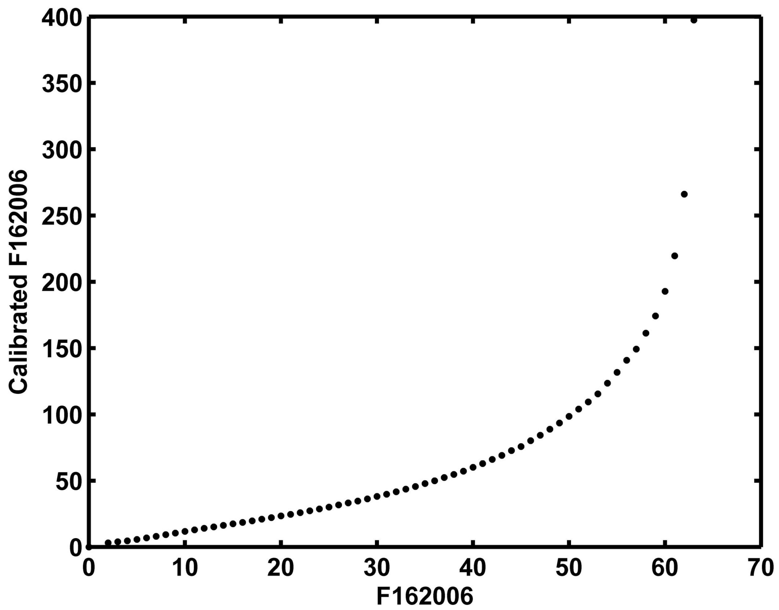
The 2006 RCNL image is one without saturation that we could obtain. The original images needed to produce this calibrated image were obtained by satellite F16; thus, we selected the SNL image coded F162006 as the corresponding data to determine where the critical point was. To this end, we performed two tests, one of which is similar to that carried out in [22]. The other test was to examine the distribution rules of the DNs of the two images. First, the relationship between the mean of the DNs of the 2006 RCNL image and the corresponding DN of the 2006 SNL image F162006 at the pixel scale (Figure 1) was tested. This showed that the relationship remains linear roughly when the DN < 50, and becomes increasingly distorted the higher the DN is over 50. To quantify this change, we performed a set of regressions. The regression formula is as follows:
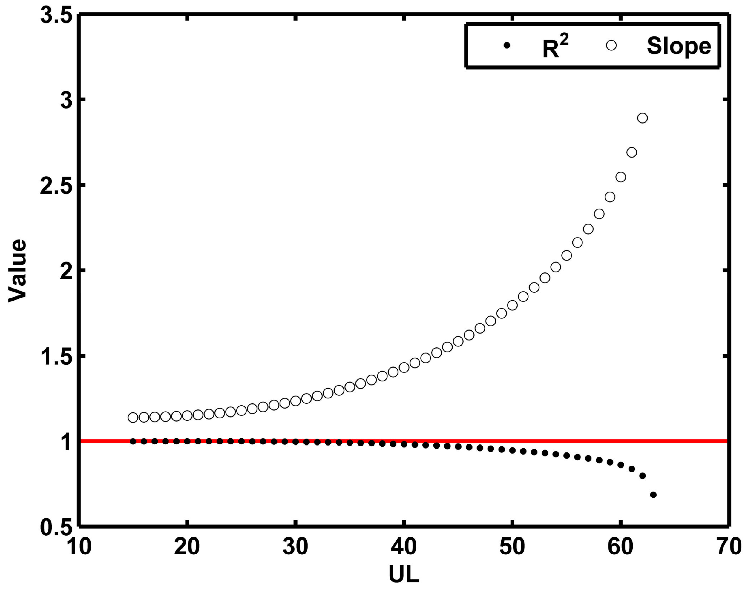
where slope is the coefficient of the DN of the SNL image. UL is the upper limit of the DN of the SNL image, which was set from 15 to 63 in each round of regression. We then plotted the coefficient of determination (R2) and the coefficient slope for each regression (Figure 2). In the ideal situation, both indicators should be close to 1. However, the R2 decreases sharply when the UL is greater than 50, and the coefficient slope gets further away from 1 when the UL exceeds 50. This indicates that the linear relationship between the DNs of the two images disappears when the DN is above 50.
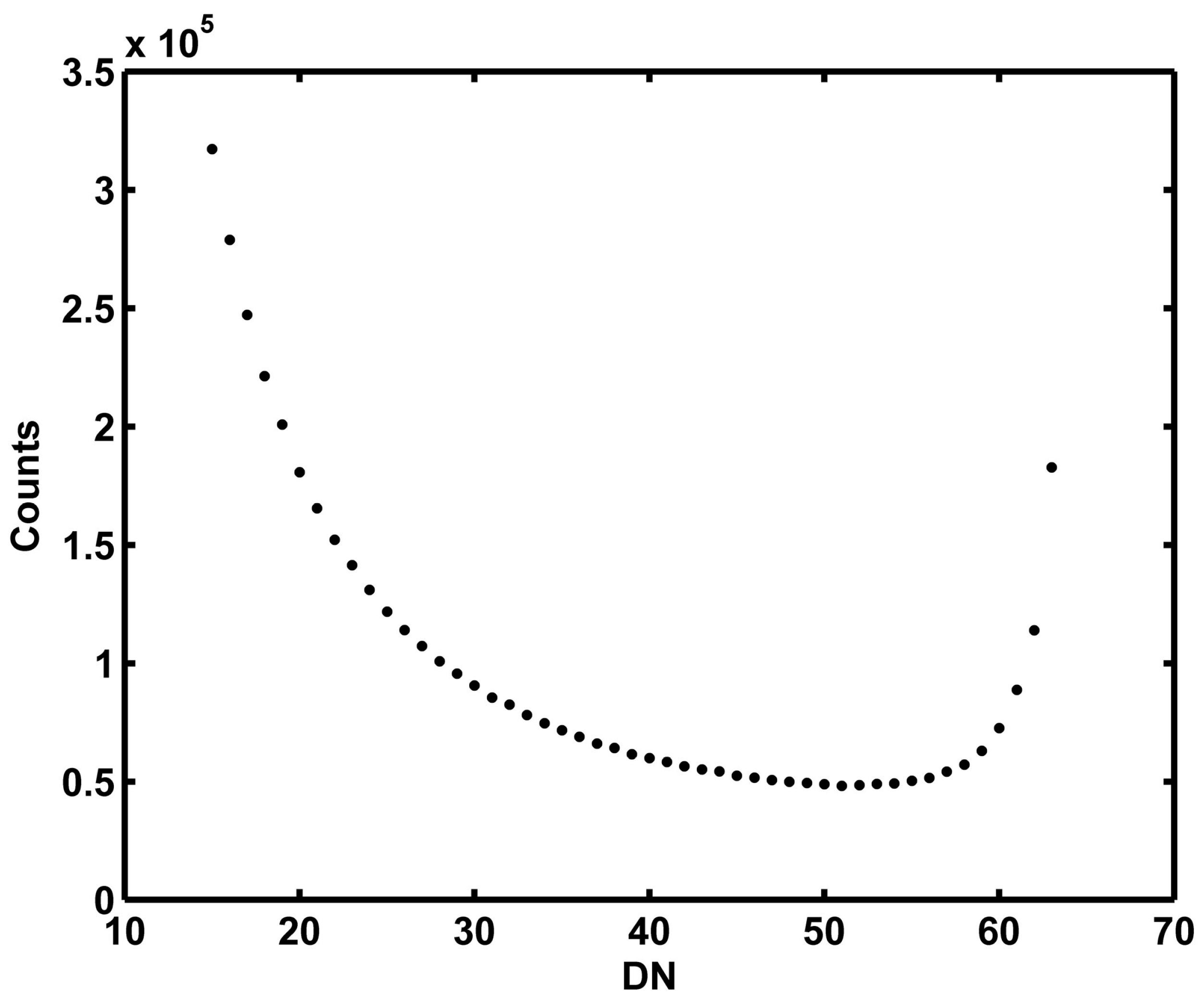
Next, the distribution rules of the DN values of the 2006 RCNL image and the 2006 SNL image were examined (Figure 3 and Figure 4). These show that when the DN > 50, especially above 55, the distribution rule of the DNs of pixels in the 2006 SNL image becomes badly distorted due to the saturation problem, compared with that of the 2006 RCNL image.
It can be concluded from both tests that pixels may start to become saturated when the DN is larger than 50, or at most 55, and that the saturation is more serious when the DN is larger. To be prudent, we classified all pixels into three categories: unsaturated pixels (DN ≤ 50), slightly saturated pixels (50 < DN ≤ 55), and severely saturated pixels (DN > 55). The unsaturated part needs no correction, while the severely saturated part will be corrected later. Strictly speaking, the slightly saturated part should also be corrected; however, any kind of correction may introduce new errors, and we cannot guarantee, for the middle range, that the amelioration by correction is larger than the error caused. Consequently, we decided not to correct the slightly saturated part in this study.
3. Exploring the Relationship between the NDVI and Nighttime Lights
Previous study results support the idea that the NDVI or the similar Net Primary Productivity (NPP) is negatively correlated with urban characteristics. One indicator of this is the intensity of nighttime lights [18,26,27]. It seems that the NDVI is a good resource to help correct the saturation problem of nighttime lights data. Although there appears to be no empirical study about the quantitative relationship between the NDVI and nighttime lights until now, we suspect that the real NDVI, without further processing, is not suitable for saturation correction at the national or global scale because it varies significantly according to the local climate [28,29,30]. For instance, the real NDVI for a city located in an arid area may be quite different from that for a similar city in a humid region. Therefore, RNDVI (relative NDVI) for urban areas, which is defined below to eliminate disturbance due to local natural factors, is suggested as an alternative measure.
where interpolated NDVI means the NDVI interpolated by NDVI of non-urban areas, which generally reflects local climate conditions.
Our major data source for RNDVI was the SPOT-VGT images (http://free.vgt.vito.be). These are 10-day composites (36 images per year) with a 1-km spatial resolution. After processing the primary VGT data into NDVI, we retrieved the maximum value of the 36 images for year 2006 for each pixel [31]. We thus obtained a yearly composite (real NDVI). To create the RNDVI image, we also need the 2006 SNL image to assist in determining which pixel belongs to urban regions and should be updated by RNDVI. In this study, we took DN = 20 as the threshold, which means that the interpolation should be performed for pixels with DN > 20 using the NDVI of pixels with DN ≤ 20. If the threshold is lower, the area to be interpolated would be larger; thus the precision of the interpolation would be greatly reduced. If the threshold is higher, the pixels to be analyzed later by regression would be greatly decreased. We did some calculations and found that DN = 20 was a good compromise for China and it was thus adopted. Different regions may have different optimal thresholds and thus relevant calculations should be performed to help determine it. With respect to the interpolation method, we adopted the natural neighbor interpolation based on its simplicity of calculation and rationality of interpolation results. In addition, the extremely low NDVI of water bodies should be set to null before interpolation, otherwise the interpolation results would be severely influenced. The interpolation was processed using ArcGIS 10.2, and the procedure is shown in the following flowchart (Figure 5).
Figure 6 and Figure 7 are the real NDVI and RNDVI for China, which suggests that RNDVI is an indicator without natural noises, and better reflects the degree of human activities than the real NDVI. Further quantitative comparison is performed later in this section.
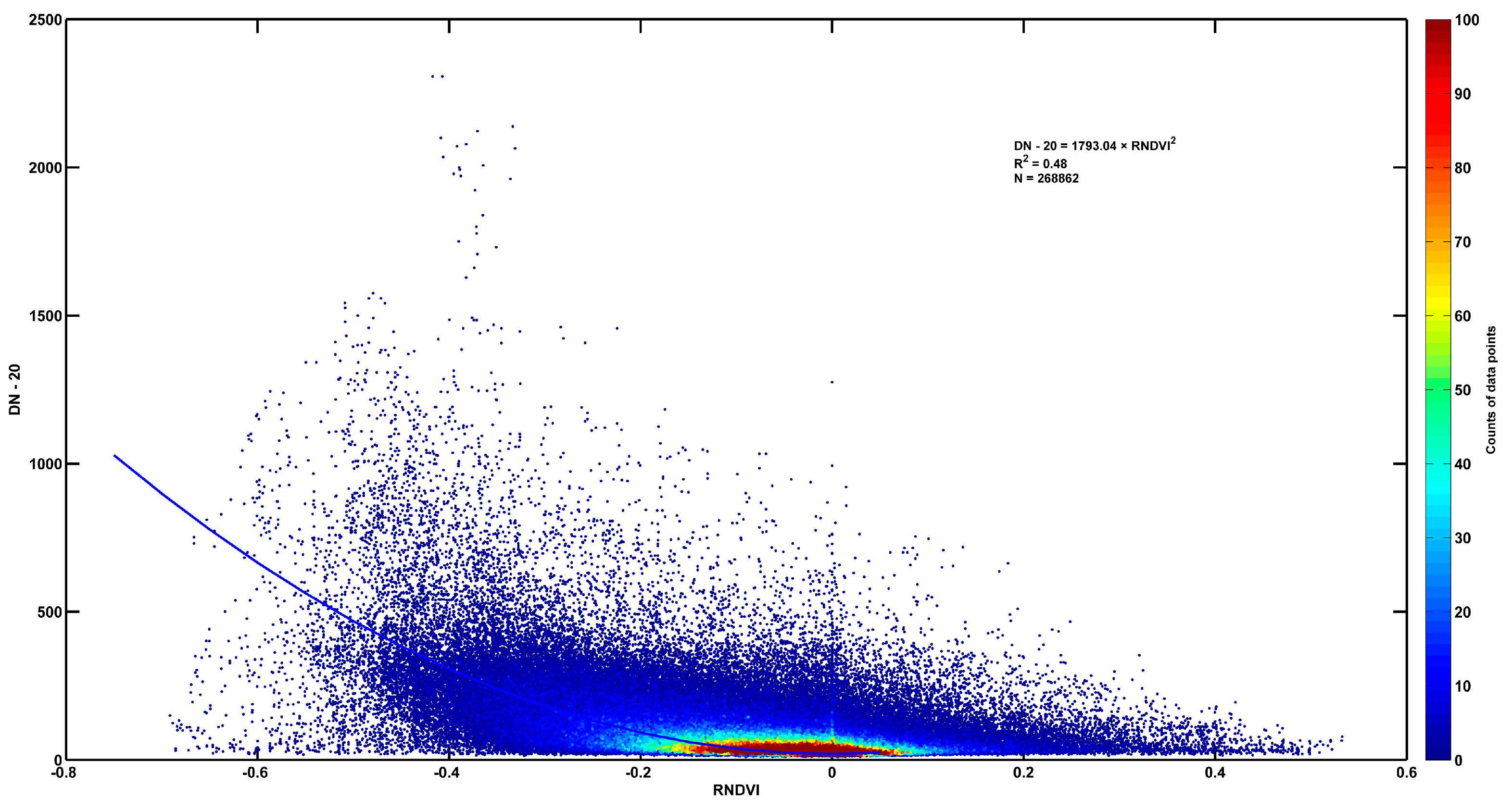
A series of regressions was performed using Stata 13.0 to identify the fittest order of function needed to describe the relationship between DN − 20 of the 2006 RCNL image and RNDVI. Ideally, RNDVI should be 0 if the DN = 20, according to the procession rule above. Consequently, the regression equation should be a homogeneous equation, namely, the constant term should be forced to be 0. The results of the linear regression, quadratic regression, and quartic regression are shown below in Table 1. Although all three regressions are significant and effective, the quadratic function depicts the relationship best and thus was selected to correct the saturated area of the 2006 SNL image.
To help prove that RNDVI is a better indicator than the real NDVI for saturation correction, more regressions were performed between the real NDVI and corresponding DNs for those pixels with DN > 20. The R2 of linear, quadratic, and quartic regressions were below 0.2 (Table 2), and were significantly lower than those of RNDVI and DN − 20 (Table 1). This demonstrates statistically that RNDVI is probably a much better indicator for correcting the saturation of nighttime lights data.
However, there are some other things we should also pay attention to. As shown in Figure 8, when RNDVI is below −0.4, the distribution of scatters seems quite discrete and with strong uncertainty, although its trend still fits the quadratic curve generally. This indicates that RNDVI, and therefore NDVI, might also suffer a “saturation problem” when it is low enough (corresponding roughly to the pixels where the DN of the nighttime lights is saturated the most severely). Therefore, the NDVI might no longer be effective for correcting light saturation when RNDVI is below −0.4. However, this problem was ignored in our study to reduce the complexity.
4. Saturation Correction Results and Evaluation
In light of the conclusion of Section 3, the quadratic function was adopted in the regression between the DN and RNDVI, and the formula is as follows:
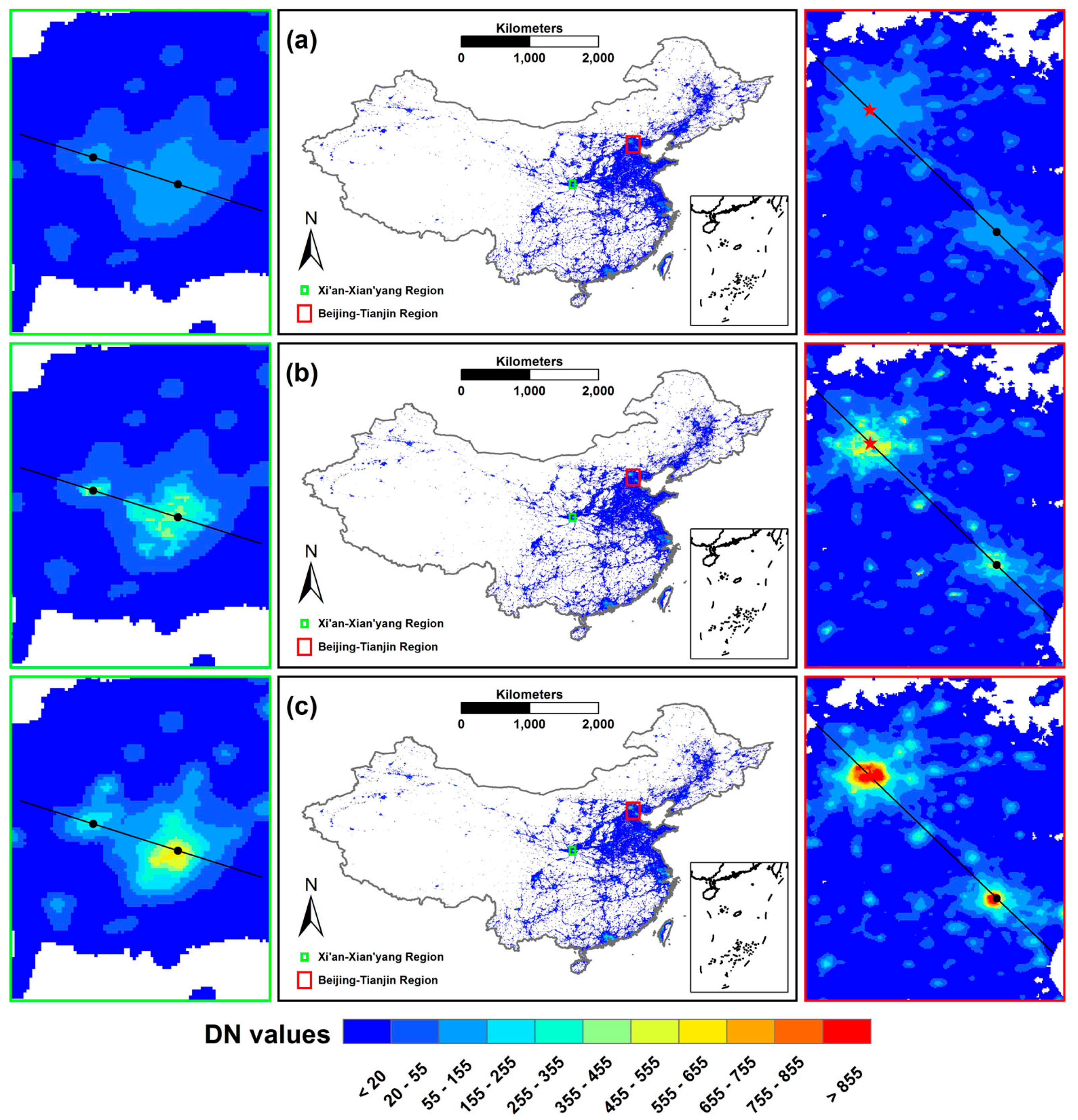
The result is significant at the 0.01 level with an R2 of 0.48. Using the Raster Calculator Tool in ArcGIS 10.2, the corrected DNs of the saturated pixels were obtained using the RNDVI image and Equation (3). If the corrected DN was lower than 55, it remained unchanged. The corrected pixels were integrated into the final corrected image with the uncorrected pixels. Figure 9 shows the final corrected nighttime lights image along with the 2006 SNL and RCNL images in China.
A total of 31,467 DNs were corrected, with the maximum DN value increased from the original 63 to 877.104. We selected the Beijing–Tianjin and Xi’an–Xian’yang regions as two examples with which to demonstrate our correction results (Figure 9). These are typical urban areas located in the north and west of China, respectively. As shown in Figure 9, the corrected image resembles the RCNL image more in terms of presenting variations and spatial details, which means that the degree of saturation of DNs in the original images of urban centers has been significantly reduced.
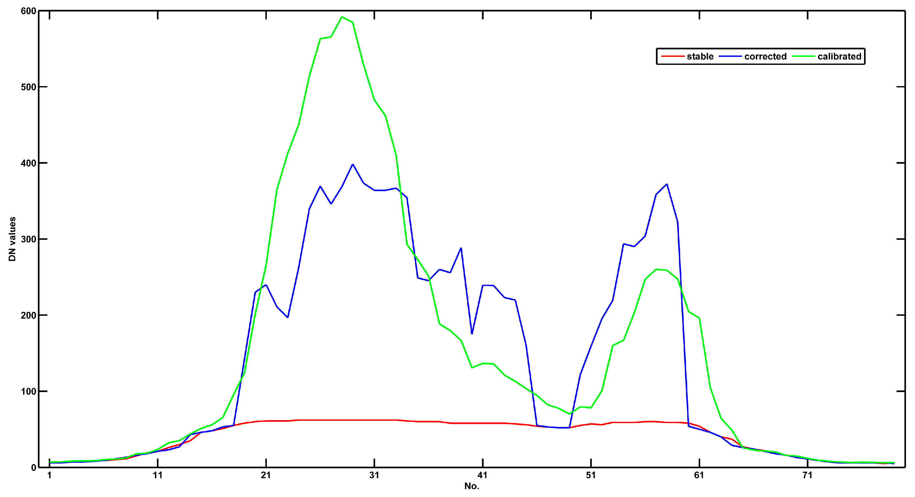
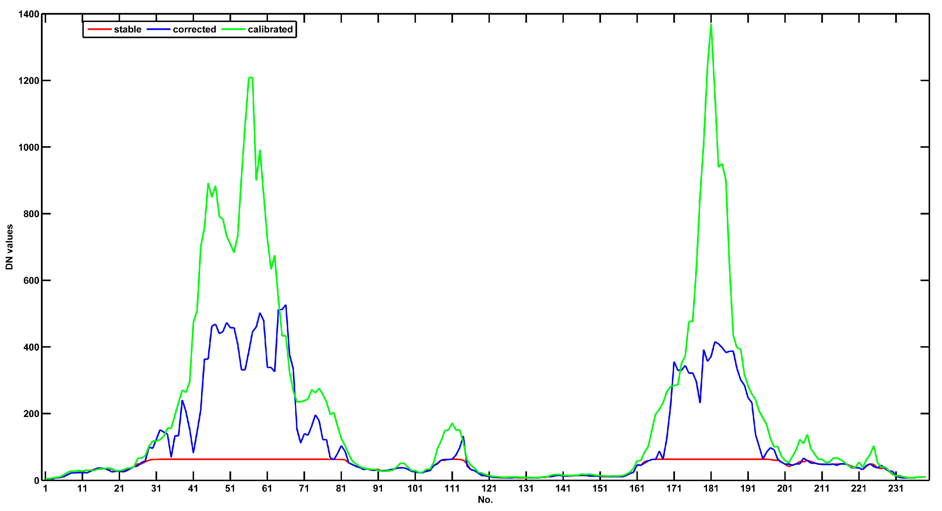
Three assessments were performed to evaluate the correction results quantitatively. First, we visually compared the corrected DN, the DN of the 2006 SNL and RCNL images from transects in the typical regions. Two groups of straight lines were added on Figure 9, one of which passed through the Beijing–Tianjin central area (40.26°N, 116.04°E) to (38.78°N, 117.57°E); the other passed through the Xi’an–Xian’yang central area (34.19°N, 109.18°E) to (34.40°N, 108.51°E). We then extracted the three groups of DN values from the corrected, 2006 SNL, and RCNL images, respectively, by the lines. Every group of DN values was exported, assigned a serial number (No.), and plotted on a curve (Figure 10 and Figure 11). The figures show that the DN values in urban centers have been significantly improved in the corrected image. The fine spatial details are successfully described, in contrast to their condition in the original images, and they are very similar to those in the calibrated images.
Next, we conducted two regressions with DN > 0. One is between the 2006 SNL and RCNL images and the other is between the corrected and 2006 RCNL images. Table 3 shows the R2 and RMSE of these two regressions, illustrating that the DNs after correction were much more relevant linearly to those of the 2006 RCNL image (R2 0. 65 vs. 0. 53 and RMSE 26.39 vs. 30.53).
In addition to the three images, we also tried to test the results using other data. In earlier studies, it was found that a high correlation exists between GDP and the accumulative DN of the unsaturated nighttime lights in a region [16]. Two regressions were also performed for provinces in China between GDP and the sums of DNs of both the corrected data and the original data. The correlation coefficient was 0.8461 for the original data, and 0.8626 for the corrected data. This also indicates that our correction is meaningful.
All of the above tests suggest that the method proposed in this study to utilize RNDVI to correct saturation for the nighttime lights image is basically effective and successful, although it only offers limited improvements. Most of the corrected DNs, however, are still smaller than they should be, especially in the core urban area (Figure 10 and Figure 11). This might have occurred for three major reasons. First, defects in the NDVI data could be to blame, as was mentioned in Section 3. RNDVI, and therefore NDVI, may suffer “saturation,” especially when lower than −0.4 (where DNs suffer the most severe saturation). Thus, it loses its authenticity and validity in these areas. The second major reason might be that not all samples follow the uniform relationship, as presumed, and not all places conform to the pattern of brighter lights along with lower NDVI. In contrast, urbanization in some areas might result in more vegetation cover [18]. The third reason could be that the slightly saturated samples (50 < DN ≤ 55 for F162006) have not been corrected at all.
5. Discussion and Conclusions
There is a growing need for more detailed and accurate characterization of urban areas at global or national scales. Nighttime lights data obtained by DMSP/OLS are some of the data most widely used to depict urban characteristics. However, the light saturation problem in urban cores has hindered its application. Many scholars have endeavored to alleviate it by developing a lot of different methods. For DMSP/OLS images, this study concludes, pixels might start to suffer saturation when the DN > 50, or at most 55, and the saturation is more serious when the DN is larger. To be prudent, we classified all pixels into three categories: unsaturated pixels (DN ≤ 50), slightly saturated pixels (50 < DN ≤ 55) and severely saturated pixels (DN > 55). Considering that any correction may introduce new errors, we could not guarantee that the amelioration by correction would cover the error it might introduce to the middle range, so we decided not to correct the slightly saturated pixels in this study.
RNDVI, derived by subtracting the interpolated NDVI from the real NDVI, was utilized to correct the saturation of nighttime lights images. RNDVI is significantly better at reflecting the degree of human activity compared to the real NDVI because it eliminates background noise. DN = 20 was set as the threshold to distinguish urban and non-urban areas, with the intention to have enough samples in the two categories for significance of regressions and low interpolation biases. Generally, quadratic functions described well the relationship between the intensity of nighttime lights and RNDVI. All of the evaluations performed proved that the proposed saturation correction method was effective at abating the saturation problem. Nevertheless, we should also note that the correction is not yet sufficient in core urban areas, which might have three causes: the “saturation” of RNDVI, statistical errors, and ignorance about slightly saturated pixels.
In terms of the application of our work, it was mainly focused on demonstration of a new saturation correction method for nighttime lights data from DMSP/OLS and could be extended to other regions and other years. Both DMSP/OLS nighttime lights data and SPOT-VGT NDVI data are globally available. Therefore, it is only necessary to undergo the procedure described in Figure 5 when applying the method to other regions. Applying the method directly at a global scale might obtain a statistically significant result but is not recommended. The reason is that not all places conform to the pattern of brighter lights along with lower NDVI. Therefore, application at national or regional scale is better. Temporally, the method could be applied to other adjacent years with SNL images but without RCNL images, under the assumption that the relationship between DN − 20 and RNDVI does not change with years. However, caution should be observed because the World Stable Lights dataset lacks comparability. SNL images from other years should be adjusted to the 2006 SNL image through inter-calibration prior to saturation correction. The invariant region method is one of the most widely used methods for inter-calibration and thus could be utilized. As a benefit from the preliminary inter-calibration, the final saturation corrected images of different years would surely be comparable. Because we will utilize different NDVI data for different years, it is not difficult to understand that the final saturation-corrected images will also present different light intensity gradients in the same saturated areas, which is an advantage over previous methods based on RCNL images only.
Numerous studies have used NDVI or relevant indicators to monitor land cover dynamics at the global or national scales. RNDVI, as proposed and used in this study, can more directly characterize the impact of human activities on vegetation when compared with the real NDVI. It is suggested that vegetation density is negatively related to temperature in certain areas [32]. However, these relationships vary a lot in different regions with various natural conditions. Relative vegetation indexes may provide the potential for achieving a unified framework for field studies. Furthermore, in the domain of remote sensing, saturation problems are not rare because every man-made sensor has some detection deficiency. No man-made sensor has perfect spatial, temporal, and radiant resolution. For example, particles with aerodynamic diameters of < 2.5 μm, also called PM2.5, tend to suffer a similar problem at high densities [33]. Sometimes the problem may be severe enough to impede the application of the data, in which case it seems wise to utilize other data relevant to the saturated data to help correct them. This kind of practice is meaningful, although it is unlikely to be perfect.
Acknowledgments
This study was financially supported by the National Natural Science Foundation of China (No. 41330747 and No. 41471370).
Author Contributions
Zheng Wang and Jiansheng Wu conceived and designed the experiments; Fei Yao performed the experiments; Fei Yao and Weifeng Li analyzed the data; Fei Yao contributed analysis tools; Zheng Wang wrote the paper.
Conflicts of Interest
The authors declare no conflict of interest. The founding sponsors had no role in the design of the study; in the collection, analyses, or interpretation of data; in the writing of the manuscript, and in the decision to publish the results.
References
- Elvidge, C.D.; Baugh, K.E.; Kihn, E.A.; Kroehl, H.W.; Davis, E.R.; Davis, C.W. Relation between satellite observed visible-near infrared emissions, population, economic activity and electric power consumption. Int. J. Remote Sens. 1997, 18, 1373–1379. [Google Scholar] [CrossRef]
- Doll, C.N.H.; Muller, J.P.; Morley, J.G. Mapping regional economic activity from night-time light satellite imagery. Ecol. Econ. 2006, 57, 75–92. [Google Scholar] [CrossRef]
- Doll, C.N.H.; Muller, J.P.; Elvidge, C. Night-time imagery as a tool for global mapping of socioeconomic parameters and greenhouse gas emissions. Ambio 2000, 29, 157–162. [Google Scholar] [CrossRef]
- Elvidge, C.D.; Baugh, K.E.; Anderson, S.J.; Sutton, P.C.; Ghosh, T. The night light development index (NLDI): A spatially explicit measure of human development from satellite data. Soc. Geogr. Discuss. 2012, 7, 23–35. [Google Scholar] [CrossRef]
- Elvidge, C.D.; Ziskin, D.; Baugh, K.E.; Tuttle, B.T.; Ghosh, T.; Pack, D.W.; Erwin, E.H.; Zhizhin, M. A fifteen year record of global natural gas flaring derived from satellite data. Energies 2009, 2, 595–622. [Google Scholar] [CrossRef]
- Ghosh, T.; Anderson, S.; Powell, R.L.; Sutton, P.C.; Elvidge, C.D. Estimation of Mexico’s informal economy and remittances using nighttime imagery. Remote Sens.-Basel 2009, 1, 418–444. [Google Scholar] [CrossRef]
- Imhoff, M.L.; Bounoua, L.; DeFries, R.; Lawrence, W.T.; Stutzer, D.; Tucker, C.J.; Ricketts, T. The consequences of urban land transformation on net primary productivity in the united states. Remote Sens. Environ. 2004, 89, 434–443. [Google Scholar] [CrossRef]
- Small, C.; Elvidge, C.D.; Balk, D.; Montgomery, M. Spatial scaling of stable night lights. Remote Sens. Environ. 2011, 115, 269–280. [Google Scholar] [CrossRef]
- Small, C.; Pozzi, F.; Elvidge, C.D. Spatial analysis of global urban extent from DMSP-OLS night lights. Remote Sens. Environ. 2005, 96, 277–291. [Google Scholar] [CrossRef]
- Sutton, P.; Roberts, D.; Elvidge, C.; Baugh, K. Census from heaven: An estimate of the global human population using night-time satellite imagery. Int. J. Remote Sens. 2001, 22, 3061–3076. [Google Scholar] [CrossRef]
- Sutton, P.C. A scale-adjusted measure of “urban sprawl” using nighttime satellite imagery. Remote Sens. Environ. 2003, 86, 353–369. [Google Scholar] [CrossRef]
- Sutton, P.C.; Costanza, R. Global estimates of market and non-market values derived from nighttime satellite imagery, land cover, and ecosystem service valuation. Ecol. Econ. 2002, 41, 509–527. [Google Scholar] [CrossRef]
- Elvidge, C.; Baugh, K.; Zhizhin, M.; Hsu, F. Why VIIRS data are superior to DMSP for mapping nighttime lights. Proc. Asia-Pac. Adv. Netw. 2013, 35, 62–69. [Google Scholar] [CrossRef]
- Baugh, K.; Elvidge, C.; Ghosh, T.; Ziskin, D. Development of a 2009 stable lights product using DMSP-OLS data. Proc. Asia-Pac. Adv. Netw. 2010, 30, 114–130. [Google Scholar] [CrossRef]
- Elvidge, C.D.; Tuttle, B.T.; Sutton, P.S.; Baugh, K.E.; Howard, A.T.; Milesi, C.; Bhaduri, B.L.; Nemani, R. Global distribution and density of constructed impervious surfaces. Sens.-Basel 2007, 7, 1962–1979. [Google Scholar] [CrossRef]
- Elvidge, C.D.; Baugh, K.E.; Dietz, J.B.; Bland, T.; Sutton, P.C.; Kroehl, H.W. Radiance calibration of DMSP-OLS low-light imaging data of human settlements. Remote Sens. Environ. 1999, 68, 77–88. [Google Scholar] [CrossRef]
- Ziskin, D.; Baugh, K.; Feng, C.; Ghosh, T.; Elvidge, C. Methods used for the 2006 radiance lights. Proc. Asia-Pac. Adv. Netw. 2010, 30, 131–142. [Google Scholar] [CrossRef]
- Zhang, Q.L.; Schaaf, C.; Seto, K.C. The vegetation adjusted ntl urban index: A new approach to reduce saturation and increase variation in nighttime luminosity. Remote Sens. Environ. 2013, 129, 32–41. [Google Scholar] [CrossRef]
- Hara, M.; Okada, S.; Ichizuka, M.; Shigehara, K.; Moriyama, T.; Sugimori, Y. Monitoring of fishing lights intensity for squid fishing vessels by means of DMSP/OLS nightlight imagery. J. Adv. Mar. Sci. Technol. Soc. 2004, 9, 99–108. [Google Scholar]
- Letu, H.; Hara, M.; Yagi, H.; Naoki, K.; Tana, G.; Nishio, F.; Shuhei, O. Estimating energy consumption from night-time DMPS/OLS imagery after correcting for saturation effects. Int. J. Remote Sens. 2010, 31, 4443–4458. [Google Scholar] [CrossRef]
- Wu, J.S.; Wang, Z.; Li, W.F.; Peng, J. Exploring factors affecting the relationship between light consumption and GDP based on DMSP/OLS nighttime satellite imagery. Remote Sens. Environ. 2013, 134, 111–119. [Google Scholar] [CrossRef]
- Letu, H.; Hara, M.; Tana, G.; Nishio, F. A saturated light correction method for DMSP/OLS nighttime satellite imagery. IEEE Trans. Geosci Remote 2012, 50, 389–396. [Google Scholar] [CrossRef]
- Cao, X.; Chen, J.; Imura, H.; Higashi, O. A svm-based method to extract urban areas from DMSP-OLS and SPOT VGT data. Remote Sens. Environ. 2009, 113, 2205–2209. [Google Scholar] [CrossRef]
- Lu, D.S.; Tian, H.Q.; Zhou, G.M.; Ge, H.L. Regional mapping of human settlements in Southeastern China with multisensor remotely sensed data. Remote Sens. Environ. 2008, 112, 3668–3679. [Google Scholar] [CrossRef]
- Pandey, B.; Joshi, P.K.; Seto, K.C. Monitoring urbanization dynamics in India using DMSP/OLS night time lights and SPOT-VGT data. Int. J. Appl. Earth Obs. Geoinform. 2013, 23, 49–61. [Google Scholar] [CrossRef]
- Milesi, C.; Elvidge, C.D.; Nemani, R.R.; Running, S.W. Assessing the impact of urban land development on net primary productivity in the Southeastern United States. Remote Sens. Environ. 2003, 86, 401–410. [Google Scholar] [CrossRef]
- Zhao, N.; Currit, N.; Samson, E. Net primary production and gross domestic product in China derived from satellite imagery. Ecol. Econ. 2011, 70, 921–928. [Google Scholar] [CrossRef]
- Bounoua, L.; Collatz, G.J.; Los, S.O.; Sellers, P.J.; Dazlich, D.A.; Tucker, C.J.; Randall, D.A. Sensitivity of climate to changes in NDVI. J. Clim. 2000, 13, 2277–2292. [Google Scholar] [CrossRef]
- Ichii, K.; Kawabata, A.; Yamaguchi, Y. Global correlation analysis for NDVI and climatic variables and NDVI trends: 1982–1990. Int. J. Remote Sens. 2002, 23, 3873–3878. [Google Scholar] [CrossRef]
- Potter, C.S.; Brooks, V. Global analysis of empirical relations between annual climate and seasonality of NDVI. Int. J. Remote Sens. 1998, 19, 2921–2948. [Google Scholar] [CrossRef]
- Hope, A.S.; Boynton, W.L.; Stow, D.A.; Douglas, D.C. Interannual growth dynamics of vegetation in the kuparuk river watershed, Alaska based on the normalized difference vegetation index. Int. J. Remote Sens. 2003, 24, 3413–3425. [Google Scholar] [CrossRef]
- Xu, H.Q.; Chen, B.Q. Remote sensing of the urban heat island and its changes in Xiamen city of SE china. J. Environ. Sci. China 2004, 16, 276–281. [Google Scholar] [PubMed]
- Hoff, R.M.; Christopher, S.A. Remote sensing of particulate pollution from space: Have we reached the promised land? J. Air Waste Manag. Assoc. 2009, 59, 645–675. [Google Scholar] [PubMed]
Figure 1.
Relationship between the mean of the DNs of the 2006 RCNL image and the corresponding DN of the 2006 SNL image F162006 at pixel scale: The original linear relationship is distorted when the DN is above 50 and becomes increasingly distorted the higher the DN is over 50.
Figure 1.
Relationship between the mean of the DNs of the 2006 RCNL image and the corresponding DN of the 2006 SNL image F162006 at pixel scale: The original linear relationship is distorted when the DN is above 50 and becomes increasingly distorted the higher the DN is over 50.

Figure 2.
Change curves of the R2 and the coefficient slope of regressions when pixels with DN ≤ UL are added into the regression gradually: The R2 decreases sharply when UL > 50, and the coefficient slope gets further away from 1 when UL > 50.
Figure 2.
Change curves of the R2 and the coefficient slope of regressions when pixels with DN ≤ UL are added into the regression gradually: The R2 decreases sharply when UL > 50, and the coefficient slope gets further away from 1 when UL > 50.

Figure 3.
Distribution rule of DN values of the 2006 RCNL image (dots for DN < 15 and DN > 120 have been omitted in the figure to better show the shape of the curve when the DN is close to 63).
Figure 3.
Distribution rule of DN values of the 2006 RCNL image (dots for DN < 15 and DN > 120 have been omitted in the figure to better show the shape of the curve when the DN is close to 63).
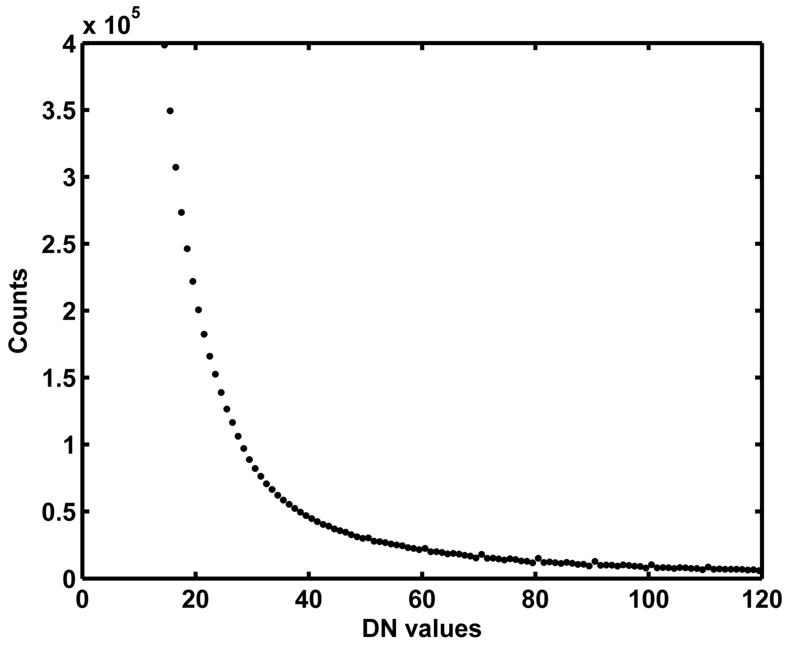
Figure 4.
Distribution rule of the DNs of the 2006 SNL image F162006 (dots for DN < 15 have been omitted in the figure to better show the shape of the curve).
Figure 4.
Distribution rule of the DNs of the 2006 SNL image F162006 (dots for DN < 15 have been omitted in the figure to better show the shape of the curve).

Figure 5.
Flowchart of the proposed method.

Figure 6.
Real NDVI in China in 2006.
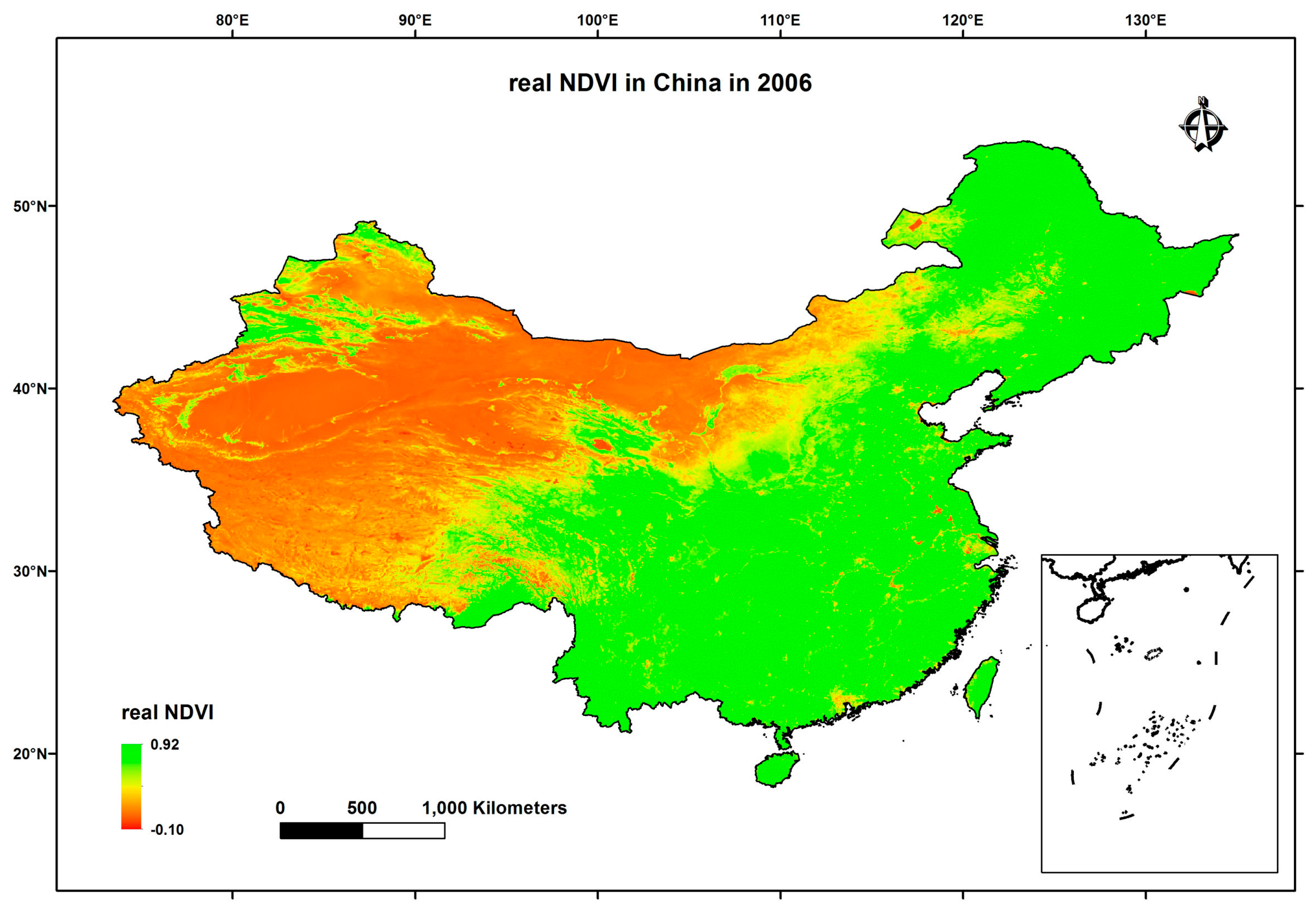
Figure 7.
RNDVI in China in 2006.
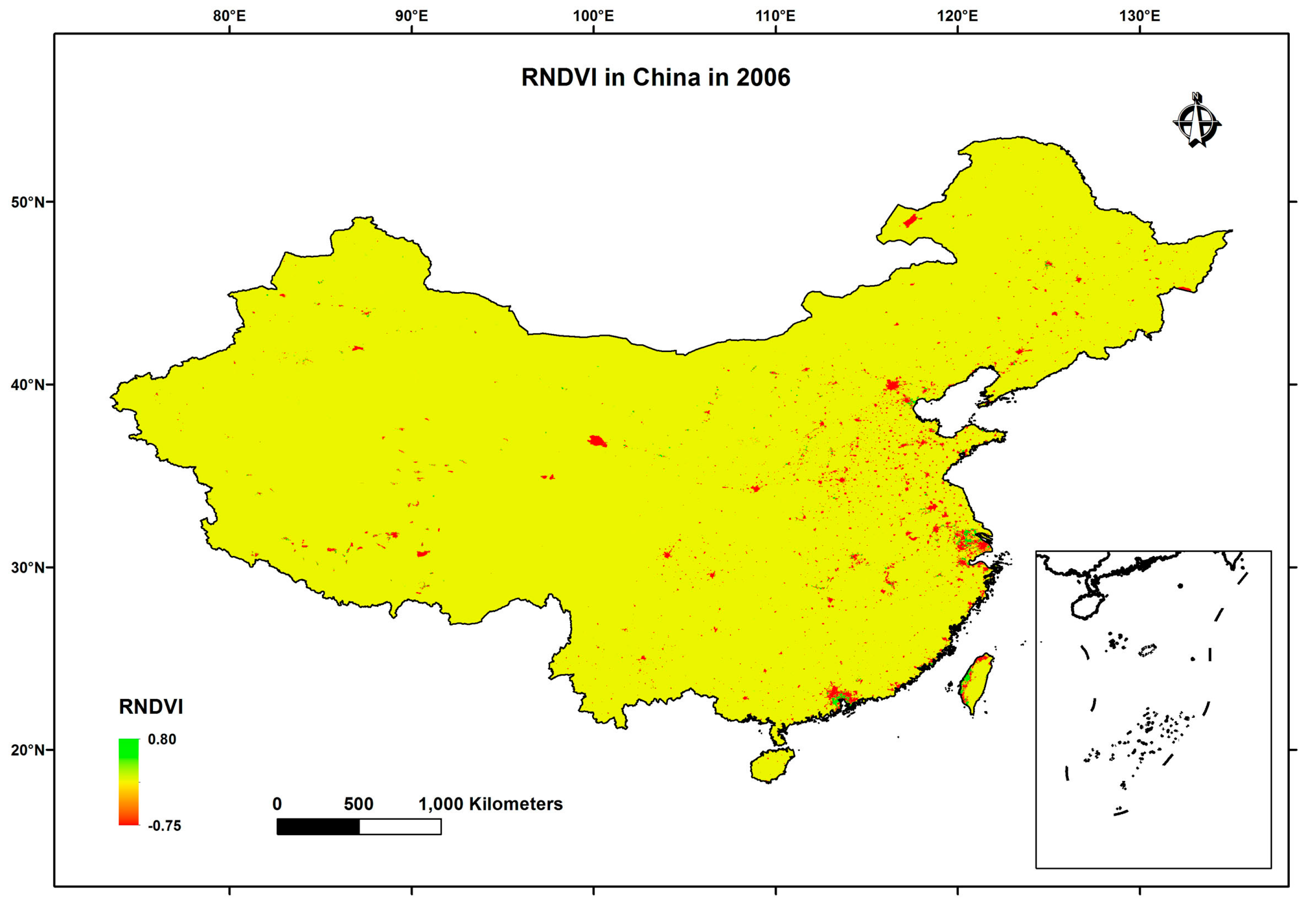
Figure 8.
Scatter plot for DN − 20 of the 2006 RCNL image and RNDVI.

Figure 9.
Nighttime lights images before and after saturation correction. (a–c) Charts correspond to the 2006 SNL image, corrected image, and RCNL image, respectively.
Figure 9.
Nighttime lights images before and after saturation correction. (a–c) Charts correspond to the 2006 SNL image, corrected image, and RCNL image, respectively.

Figure 10.
DN value curves in the corrected (blue), 2006 SNL (red) and RCNL (green) images extracted by the straight line (from (40.26°N, 116.04°E) to (38.78°N, 117.57°E), Beijing–Tianjin region).
Figure 10.
DN value curves in the corrected (blue), 2006 SNL (red) and RCNL (green) images extracted by the straight line (from (40.26°N, 116.04°E) to (38.78°N, 117.57°E), Beijing–Tianjin region).

Figure 11.
DN value curves in the corrected (blue), 2006 SNL (red) and RCNL (green) images extracted by the straight line (from (34.19°N, 109.18°E) to (34.40°N, 108.51°E), Xi’an–Xianyang region).
Figure 11.
DN value curves in the corrected (blue), 2006 SNL (red) and RCNL (green) images extracted by the straight line (from (34.19°N, 109.18°E) to (34.40°N, 108.51°E), Xi’an–Xianyang region).

Table 1.
Results of different order regressions between DN − 20 and RNDVI for the 2006 RCNL image.
| R2 | Coefficient | |
|---|---|---|
| RNDVI | 0.42 | −534.56 |
| RNDVI2 | 0.48 | 1793.04 |
| RNDVI4 | 0.29 | 7554.81 |
Table 2.
Results of different order regressions between DN − 20 and the real NDVI for the 2006 RCNL image.
Table 2.
Results of different order regressions between DN − 20 and the real NDVI for the 2006 RCNL image.
| R2 | Coefficient | |
|---|---|---|
| NDVI | 0.14 | 77.89 |
| NDVI2 | 0.08 | 90.90 |
| NDVI4 | 0.04 | 120.68 |
Table 3.
Results of the regression between the DNs of the 2006 RCNL image and those of the other images.
Table 3.
Results of the regression between the DNs of the 2006 RCNL image and those of the other images.
| 2006 SNL Image | Corrected Image | |
|---|---|---|
| R2 | 0.53 | 0.65 |
| RMSE | 30.53 | 26.39 |
© 2017 by the authors. Licensee MDPI, Basel, Switzerland. This article is an open access article distributed under the terms and conditions of the Creative Commons Attribution (CC BY) license (http://creativecommons.org/licenses/by/4.0/).
Share and Cite
MDPI and ACS Style
Wang, Z.; Yao, F.; Li, W.; Wu, A.J. Saturation Correction for Nighttime Lights Data Based on the Relative NDVI. Remote Sens. 2017, 9, 759. https://doi.org/10.3390/rs9070759
AMA Style
Wang Z, Yao F, Li W, Wu AJ. Saturation Correction for Nighttime Lights Data Based on the Relative NDVI. Remote Sensing. 2017; 9(7):759. https://doi.org/10.3390/rs9070759
Chicago/Turabian StyleWang, Zheng, Fei Yao, Weifeng Li, and And Jiansheng Wu. 2017. "Saturation Correction for Nighttime Lights Data Based on the Relative NDVI" Remote Sensing 9, no. 7: 759. https://doi.org/10.3390/rs9070759
Note that from the first issue of 2016, this journal uses article numbers instead of page numbers. See further details here.