Coastal Waveform Retracking for Jason-2 Altimeter Data Based on Along-Track Echograms around the Tsushima Islands in Japan


1
School of Marine Science and Environment Engineering, Dalian Ocean University, Dalian 116023, China
2
Interdisciplinary Graduate School of Engineering Sciences, Kyushu University, Fukuoka 8168580, Japan
3
Research Institute for Applied Mechanics, Kyushu University, Fukuoka 8168580, Japan
*
Author to whom correspondence should be addressed.
Remote Sens. 2017, 9(7), 762; https://doi.org/10.3390/rs9070762
Submission received: 27 March 2017
/
Revised: 18 July 2017
/
Accepted: 21 July 2017
/
Published: 24 July 2017
Abstract
:Although the Brown mathematical model is the standard model for waveform retracking over open oceans, due to heterogeneous surface reflections within altimeter footprints, coastal waveforms usually deviate from open ocean waveform shapes and thus cannot be directly interpreted by the Brown model. Generally, the two primary sources of heterogeneous surface reflections are land surfaces and bright targets such as calm surface water. The former reduces echo power, while the latter often produces particularly strong echoes. In previous studies, sub-waveform retrackers, which use waveform samples collected from around leading edges in order to avoid trailing edge noise, have been recommended for coastal waveform retracking. In the present study, the peaky-type noise caused by fixed-point bright targets is explicitly detected and masked using the parabolic signature in the sequential along-track waveforms (or, azimuth-range echograms). Moreover, the power deficit of waveform trailing edges caused by weak land reflections is compensated for by estimating the ratio of sea surface area within each annular footprint in order to produce pseudo-homogeneous reflected waveforms suitable for the Brown model. Using this method, altimeter waveforms measured over the Tsushima Islands in Japan by the Ocean Surface Topography Mission (OSTM)/Jason-2 satellite are retracked. Our results show that both the correlation coefficient and root mean square difference between the derived sea surface height anomalies and tide gauge records retain similar values at the open ocean (0.9 and 20 cm) level, even in areas approaching 3 km from coastlines, which is considerably improved from the 10 km correlation coefficient limit of the conventional MLE4 retracker and the 7 km sub-waveform ALES retracker limit. These values, however, depend on the topography of the study areas because the approach distance limit increases (decreases) in areas with complicated (straight) coastlines.
1. Introduction
Radar altimeters transmit modulated chirp pulses towards the sea at nadir, and then record the echoes reflected from the sea surface in an altimeter footprint [1]. The time series of the power of the echoes received by altimeters is commonly referred to as a “waveform”. Waveforms are sampled with a specific time resolution, which is 3.125 ns for the Ocean Surface Topography Mission (OSTM)/Jason-2 satellite, and each cell within a waveform is called a “gate”. Geophysical parameters are retrieved by a process called “waveform retracking”, which consists of fitting a theoretical model to the measured waveforms. Over the open ocean, the so-called Brown mathematical model [2,3] is the standard model used for this process.
As shown in Figure 1, a typical Brown waveform which is controlled by the altimeter antenna gain pattern, has a well-defined shape consisting of three parts, thermal noise, a fast-rising leading edge, and a decaying trailing edge. The fundamental parameters obtained through waveform retracking are the satellite height above the sea surface (range), the significant wave height (SWH), and the backscatter coefficient (sigma0, ), which is related to sea surface wind. Moreover, an antenna mispointing angle (ξ) parameter, which is linked to the slope of the trailing edge, has a strong impact on sigma0 estimation because it reduces the apparent backscatter coefficient for the radar antenna (i.e., any deviation of the radar aiming point from nadir).
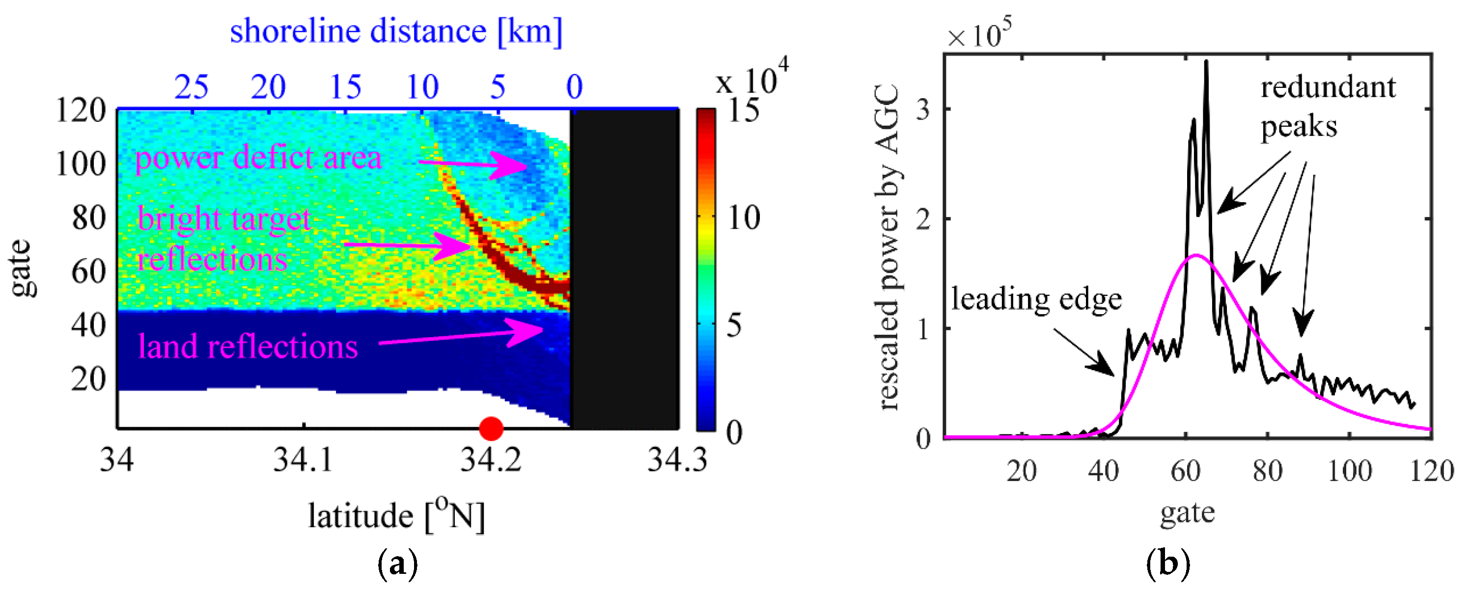
In contrast to the open ocean, waveforms collected when the altimeters operate in proximity to coastlines are often corrupted due to the heterogeneous surfaces. Figure 2a shows the along-track waveforms (or azimuth-range radar-gram; hereafter referred to as an echogram) measured by the Jason-2 altimeter over the southern Tsushima Islands in Japan (pass 36, cycle 22). Each column of the echogram represents an individual waveform at a given latitude. Waveforms in the echogram have been realigned based on the tracker movements and rescaled by the automatic gain control (AGC) of the antenna [4]. Waveforms measured over land areas are masked in the echogram because they cannot be properly realigned. As can be seen in Figure 2a, land reflections are generally significantly weaker than reflections from the sea surface [5]. This is why the trailing edge of a waveform will decay rapidly when an altimeter approaches land, thereby resulting in a power deficit area in the echogram [6]. Moreover, several bright parabolic traces can be seen at the waveform trailing edge area, which indicate that bright targets exist within the altimeter footprint.
Figure 2b shows an example of a corrupted waveform measured at the location indicated by the red point in Figure 2a (34.20°N). The black line represents the actual waveform and the red line represents the fitted waveform using the four-parameter Brown theoretical model. An unweighted least-squares estimator whose convergence is obtained through the Nelder-Mead algorithm is adopted in the present study. It is obvious that the estimated Brown waveform deviates seriously from an ideal undistorted waveform without redundant peaks around gates 60–80.
In the last couple of years, a significant amount of research has been aimed at overcoming the effect of waveform corruption on retracking over coastal zones. As a result, several dedicated parametric and non-parametric models have been proposed, a detailed review of which can be found in [7]. In some previous studies, sub-waveform retrackers [8,9,10,11], which use only the waveform samples around the leading edge rather than the full waveforms, have been recommended for coastal waveform retracking. These retrackers successfully suppress trailing edge noise, and hence extend the capabilities of waveform retracking in coastal zones closer to the shorelines. However, loss of the trailing edge during the retracking process will also reduce the precision of estimated geophysical parameters, especially for sigma0 estimation [10]. Moreover, although sub-waveform retrackers depend on the detection accuracy of the leading edge in a waveform, practically speaking, it is difficult to separate the leading edge from individual multi-peak waveforms when numerous speckles are present.
The previous concept regarding individual waveform noise detection was based on the on-board processing strategy of radar altimeters. However, more reliable detection is possible through post-processing using along-track waveforms because waveform noise at a given location can be expected to be geographically related to such noise in adjacent locations. Thus, trailing edge noise can be explicitly determined based on its spatial relationship in the echogram. Sub-waveform retrackers limit the analysis of waveform samples around the leading edge to avoid trailing edge noise. This is equivalent to limiting the altimeter footprint size near the nadir points where homogeneous sea surface conditions could be expected, even though the number of samples within the footprint is decreased. In contrast, in the present study, significant noise in the trailing edge caused by bright targets is removed or modified by using echograms. This approach will also assist in obtaining homogeneous sea surface conditions, which is necessary in order to adopt the Brown model, by keeping the number of samples within the footprints constant. A similar approach, in which bright peaks were removed by comparing them with waveforms in the adjacent open water, was examined in a recent study [12]. In the present study, however, bright targets are more explicitly detected and removed by using spatial restriction conditions in the along-track waveforms.
The remainder of this paper is organized as follows. The dataset used in the present study is presented in Section 2. Here, we selected Japan’s Tsushima Islands as our test site because it is an area where waveform corruption, such as that shown in Figure 2, is often observed. The detection of noise caused by bright targets through their parabolic signatures within an echogram is introduced in Section 3.1. In Section 3.2, compensating for the waveform trailing edge power deficit due to weak land reflection is considered. The derived along-track sea surface height anomalies (SSHAs) are validated by tide gauge measurements and compared with sensor geophysical data record (SGDR) and adaptive leading-edge sub-waveform (ALES) products in Section 4. Finally, a brief discussion and summary, focusing specifically on the geographical dependency of the results, is presented in Section 5.
2. Dataset
The 20 Hz ALES coastal altimetry product of Jason-2 around the Tsushima Islands (pass 36, as shown in Figure 3) are used in this study. This is an experimental product from the ALES processor that is included in SGDR-type files alongside the standard products and corrections. The specific description can be found at http://www.coastalt.eu/community. The dataset covers the period from July 2008 to April 2015. The coastal features of the Tsushima Islands along the Jason-2 ground track are characterized by semi-closed bays within the altimeter footprints. Because semi-closed bays often appear as bright targets in radar echograms, waveforms measured in the complicated coastlines of the study area are seriously corrupted. For comparison purposes, another track (pass 164) crossing the relatively smooth coastlines of southern Taiwan is also processed, as described in Section 5 (Figure 13).
The Global Self-Consistent, Hierarchical, High-Resolution Geography database (GSHHS) [13] is used at full resolution to determine the coastline and estimate the ocean area located within altimeter annular footprints.
Hourly tide gauge data obtained from the Japan Oceanographic Data Center (JODC) are used to validate the quality of derived along-track sea surface heights (SSHs). A temporal interpolation was performed before validation to match the JODC data with the altimeter measurements. The shortest distance between tide gauge and Jason-2 ground track is about 6 km. Since tide gauge stations are located within port waters, the tidal amplitudes registered are not the same as those for the waters outside the harbors. Such discrepancies result in considerable height differences, although their spatial scale would be large.
3. Waveform Retracking Strategy
3.1. Detection of the Noise Caused by Bright Targets
Generally, the backscatter coefficient sigma0 for radar altimeters is inversely proportional to the sea surface roughness. In particular, sigma0 will sharply increase when centimeter-scale wavelets are absent from the sea surface. Over the open ocean, occurrences of unrealistically high values of are usually referred to as “sigma-0 blooms”. These occur during low wind and calm sea conditions, or can be caused by slick sea surfaces, for example. Previous studies have shown that the occurrence of unrealistically high values of sigma0 affect almost 5% of the open ocean measurements [14].
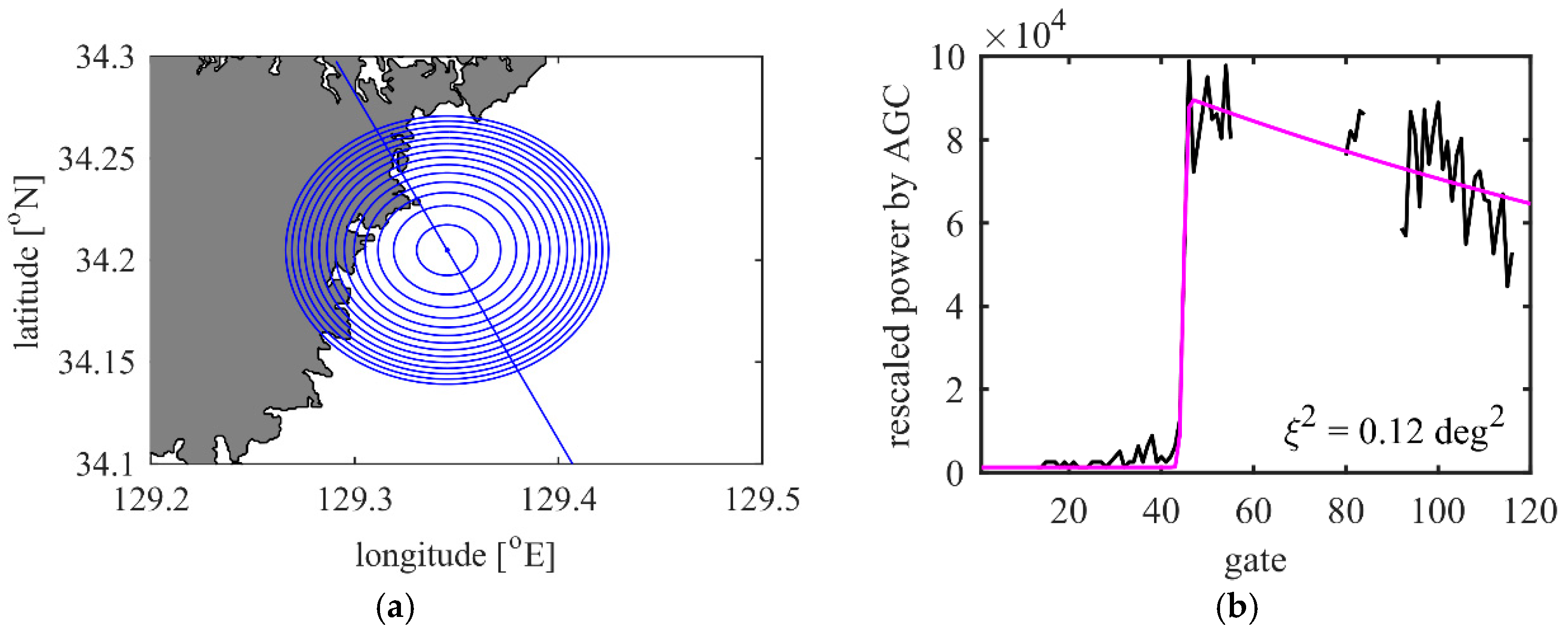
Unlike the open ocean, reflection from bright targets is one of the primary reasons for coastal waveform distortion. Parabolic signatures caused by bright targets were found in almost all of the 252 cycles of the Jason-2 echograms around the Tsushima Islands. The bright targets are related to the vertexes of the parabolic traces in the echogram, namely, the latitude and distance to the midpoint of the leading edges [6]. Using a local map (Figure 3b), the bright parabolic traces in Figure 2a are found to be reflections from semi-closed bays (circles).
As shown in Figure 2b, the redundant peaks in the waveform trailing edge significantly depart from the expected Brown waveform shape. However, since coastal waveforms are generally complicated by the presence of several redundant peaks, it is difficult to identify such corruption in an individual waveform. In this section, it is shown how echoes that are corrupted by bright targets are detected and masked utilizing their parabolic signatures within an echogram.
A point target of height above sea level located at distance from the satellite nadir will give an echo withe a round-trip delay time defined by [5]:
where is the speed of light, is the satellite height and is the Earth’s radius.
As shown in Figure 4a, represents the location at the nearest approach to a high reflector on the sea surface, while and represent the round-trip delay time and geographical distance, respectively. is a point located at a distance from , while and represent the corresponding round-trip delay time and geographical distance, respectively. Considering the geometric relationship, , Equation (1) can be expressed as:
where represents the round-trip delay time difference, and is the geographical distance between a measurement point and the nearest measurement point .
The parabolic shape determined by Equation (2) in an echogram is shown in Figure 4b. The horizontal axis represents the latitude of the satellite nadir. The vertical axis represents the round-trip delay time for the gate, and the sampling resolution is 3.125 ns for Jason-2. The vertex of the parabola is related to the location of the bright target, as seen in Figure 3b, and the parabola shape is solely determined by the altimeter’s orbital and sampling parameters.
In the present study, an iterative method is used to detect the parabolic trajectories in the echogram. It consists of three steps as follows (Figure 5):
- Step 1:
- Mark all pixels in the echogram with the 2% largest echoes, but reset those that do not exceed 10 dB. The 2% threshold is determined empirically based on the size of the study area and is approximately two times the standard deviation. The 10 dB sigma0 is used as the lower limit of the obvious noise caused by bright targets.
- Step 2:
- Shift the fixed parabolic shape in the echogram in both the latitude and gate directions, and then count the number of marked pixels along the given parabolic line.
- Step 3:
- Find the parabolic shape that provides the largest along-line number . Mask all pixels (with and without marks) along the parabolic shape if is larger than 10 or exceeds 50% of the number of pixels along the parabolic line within the study area. Repeat from Step 1, until is smaller than 10 and the ratio becomes less than 50%.
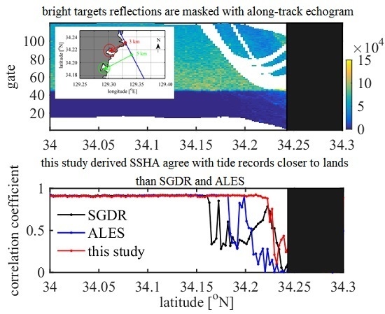
Figure 6a depicts the masked echogram for pass 36 cycle 22 of the Jason-2 data over the southern Tsushima Islands (the same as Figure 2a). Although some echoes located at the parabola tail, as shown in Figure 2a, are not particularly strong (weaker than 10 dB) due to antenna gain power decay, it is reasonable to remove all of the echoes along the same parabola that are contaminated by a strong point source. Here, four parabolic trajectories are detected and masked. These echoes will be removed in the process of waveform retracking.
The masked waveform and the fitted Brown waveform measured at 34.2°N are shown in Figure 6b. Compared to Figure 2b, the masked waveform shows strong agreement with the fitted Brown waveform. However, an unrealistic antenna mispointing angle is obtained, which will have a strong influence on the sigma0 estimation. Since the estimated mispointing angle is smaller than −0.2 deg2, according to the data-editing criterion in the standard Jason-2 product, it should be flagged as bad data. In fact, the negative mispointing angle represents a steepening of the trailing edge and cannot be interpreted as an actual physical mispointing of the instrument. In this case, the trailing edge steepening is caused by the extra power deficit due to the weak land reflection. Our power deficit compensation method is discussed in the next section.
3.2. Compensating for the Waveform Trailing Edge Power Deficit
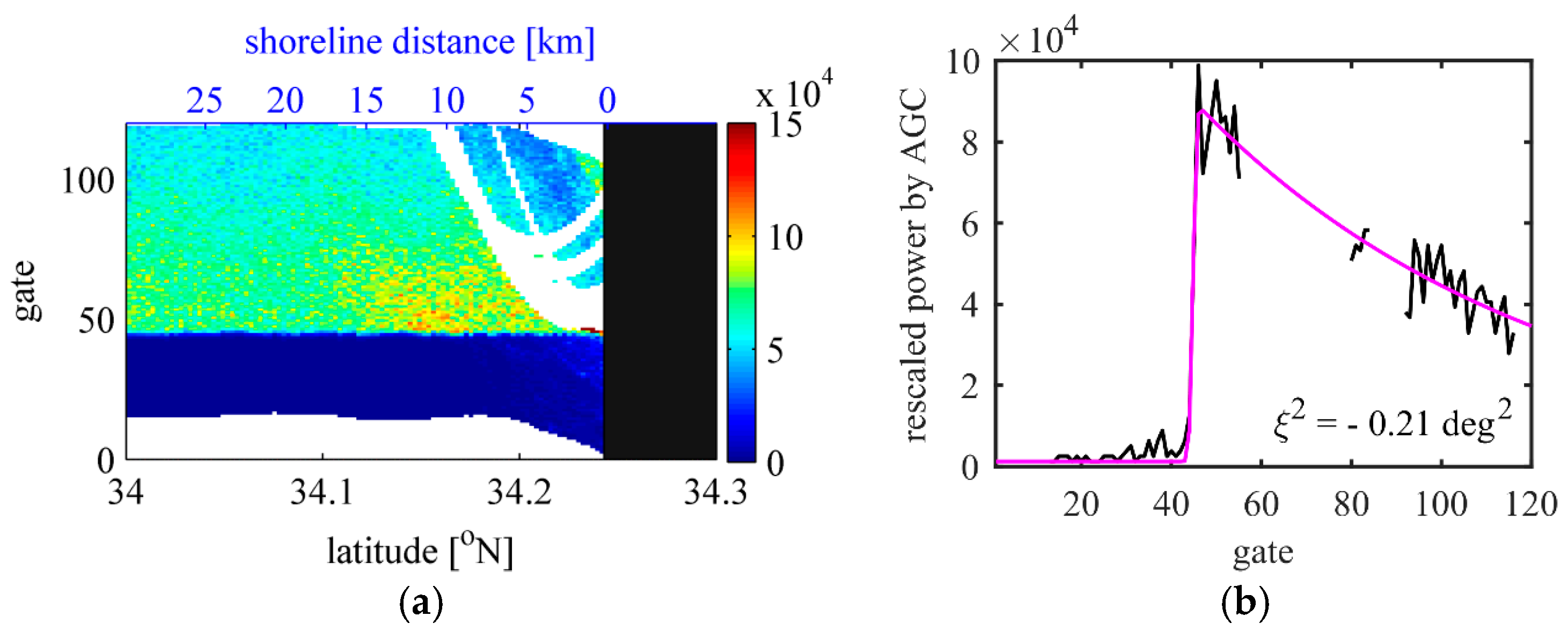
The power of an echo in a waveform is proportional to the area of the corresponding annular footprint and is controlled by the antenna beam pattern. In areas where land is located within the altimeter footprint, since the land reflection is very weak, the power is approximately proportionate to the ocean area within the annular footprint. As shown in Figure 7a, the power of the waveform trailing edge decays rapidly with decreasing sea surface area in annular footprints. Therefore, a power deficit area can be seen in the echogram, as shown in Figure 2a.
The “illumination hole” in the annular footprint that forms behind the trailing edge of the pulse is a circle with a radius and area that expand at the same rates. The area of each annular footprint, , remain unchanged and can be expressed as [15]:
where is the width of the pulse, is the speed of light, is the satellite height and is the Earth’s radius.
The sea surface area within two consecutive annular footprints, , is actually a polygon and can be estimated using the method described by Thibaut et al. [13]. In the present study, the power of each waveform trailing edge echo is roughly compensated for by dividing by the ratio, .
Figure 7a shows the annular footprints for the waveform measured at 34.20°N (red point in Figure 2a). The compensated waveform and the corresponding fitted Brown waveform are shown in Figure 7b. Compared with Figure 6b, a positive mispointing angle is obtained. The improved positive mispointing angle is found all along the track, as shown in Figure 8d. Additionally, sigma0 shows a drop near the coast before the land compensation (Figure 8c), indicating stronger wind speeds, but the SWH remains almost the same as that for the open ocean (Figure 8b). After the land compensation, it can be seen that this sigma0 drop inconsistency near the coast has been modified.
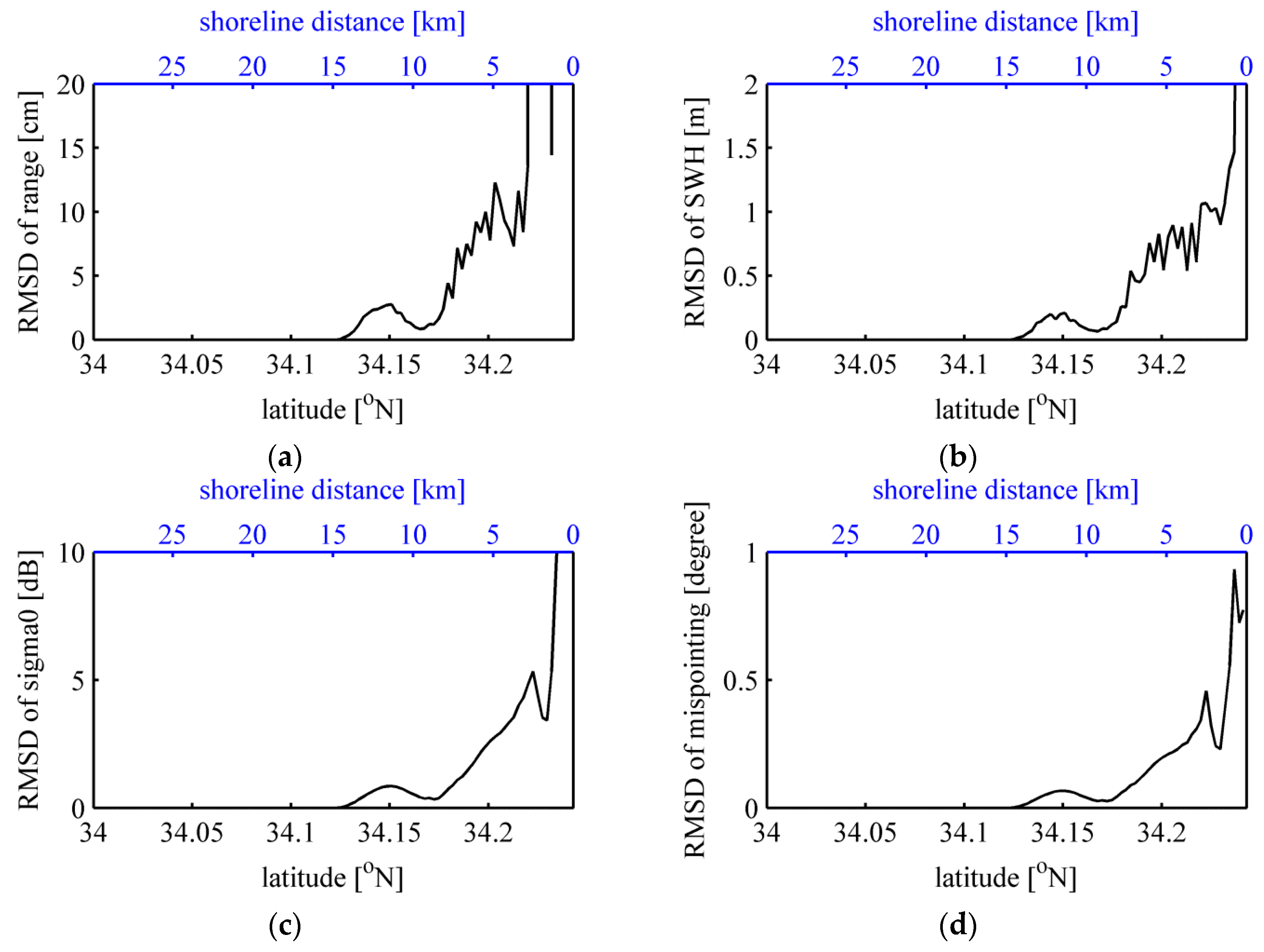
In order to quantitatively assess the effect of land compensation on waveform retracking, the root mean squared difference (RMSD) for the range, SWH, sigma0 and mispointing angle before and after land compensation are calculated (Figure 9). The results show that the power deficits due to weak land reflection seriously influence the simultaneous estimation of sigma0 and the mispointing angle. Although the waveform trailing edge is not directly used to estimate the range and SWH, the latter values are also slightly affected by the compensation for the land deficit. Therefore, in addition to of the effect of bright targets, the power deficit for the waveform trailing edge should also be carefully considered for waveform retracking around coastal areas.
4. Validation and Comparisons with Other Retrackers
In addition to the coastal zone, waveform corruption can also appear in open ocean areas where small-scale sigma0-bloom events and rain cells occur. A threshold of sigma0 is always adopted as the bloom detection criterion, e.g., the 15 dB and 18 dB criteria for the Environmental Satellite (Envisat) Radar Altimeter 2 (RA2) data discussed in [14]. Considering the sigma0 differences between various altimeters, this study uses a relative large threshold of 18 dB for Jason-2 sigma0-bloom event detection. The sigma0-bloom events are found in 18 of 252 cycles at the study area. More specifically, about 7% of the Jason-2 measurements are corrupted by the sigma0-bloom events. This rate is consistent with the study on Jason-1 data (6%) as discussed in [14]. Note that the sigma0-bloom effect on waveform retracking is out of the scope of the present study, and the 18 cycles of data have been directly removed from waveform retracking.
In order to validate the quality of the range estimation, the along-track SSHA is calculated as follows:
where is the mean SSH from cycle 1 to cycle 252. In the present study, SSH values larger than 100 m or smaller than −130 m are treated as outliers (see the Jason-2 product handbook). In order to make a comparison with tide gauge measurements, the tidal components and the inverse barometric components are not removed from either the altimeter measurements or the tide gauge records.
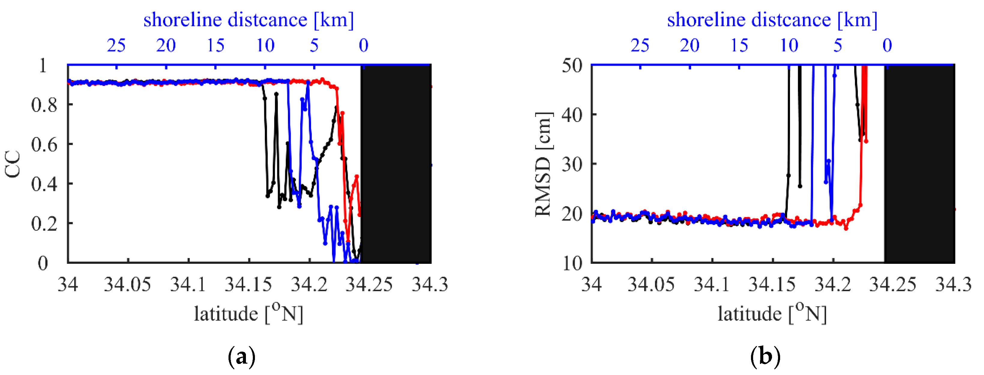
Two statistics, the correlation coefficient (CC) and the RMSD between the time series of SSHA derived from altimeter and tide gauge measurements, are used to validate the data quality as discussed in [16]. Figure 10a shows the CC variation along the track over the Tsushima Islands for the three different methods. Figure 10b is the RMSD in centimeters. These results show that the conventional ocean retracker in the SGDR product cannot provide a correct estimation within 10 km from the coastline, which corresponds approximately to the radius of the Jason-2 altimeter footprint. Meanwhile, since the ALES retracker only uses the sub-waveform around the leading edge, the noise that first appears in the waveform trailing edge has no influence on the range estimation. As a result, the ALES range estimation can be extended to about 7 km from the coastline.
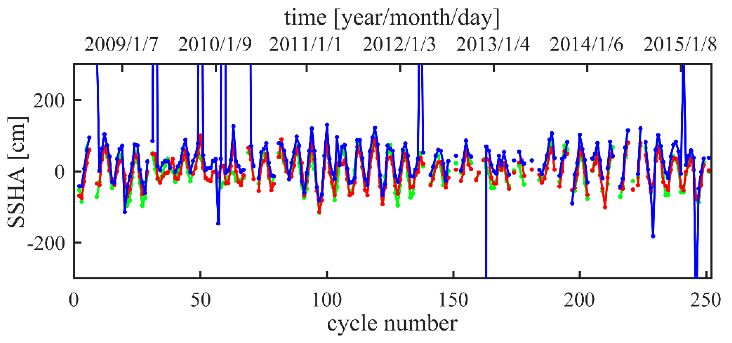
However, once the echoes used in the ALES estimation windows become corrupted, they will seriously influence the accuracy of range estimation due to reduced ALES retracker echo numbers, as shown in Figure 11. Note that all echoes within the estimation windows whose widths are determined by the SWH are used in the ALES, regardless of reliability. In the present study, however, the range is estimated based on the modified waveforms from which the effects of the two primary sources of heterogeneous surface reflections, i.e., land and bright targets, are removed. Figure 10a shows that the CC remains larger than 0.9 (99.9% confidence level) even at locations only about 3 km away from the coast. Overall, both the CC and RMSD comparison show that this method is more effective for examining areas very close to land than the ocean retracker and/or ALES retracker.
5. Discussion and Summary
Generally speaking, geophysical parameters can be correctly estimated over open ocean areas using the theoretical Brown model, which is based on the assumption of a homogeneous sea surface. However, altimeter waveforms are often corrupted at coastal zones due to heterogeneous surface reflections within the altimeter footprint. In particular, bright targets such as calm water in semi-closed bays and the vicinity of land have distinctly different scattering characteristics at nadir. Sub-waveform retrackers such as ALES use only waveform samples selected from around the leading edge in order to avoid trailing edge noise. This method is equivalent to reducing the altimeter footprint. Because homogeneous sea surface conditions are more easily anticipated for smaller footprints, such retrackers can extend their waveform retracking abilities closer to the coast. In contrast, this study considered a method of modifying waveforms in order to make them suitable for use in the Brown model.
Reflections from bright targets often appear as redundant peaks in coastal waveforms, which have sharp power variations similar to waveform leading edges (Figure 2b). When multiple redundant peaks appear in a waveform trailing edge, it is difficult to identify this noise in an individual waveform. On the other hand, reflections from a fixed-point target trace a parabola in the sequential along-track waveforms (or, azimuth-range echogram). Therefore, by utilizing the parabolic signature in the radar echogram, noise caused by bright targets can be explicitly detected and masked, as discussed in Section 3.1. When compared with an actual waveform, the masked waveform shows good agreement with the fitted Brown waveform (Figure 6b), even though the unrealistic mispointing angle indicates an extra power deficit for waveform trailing edge due to weak land reflection. Thus, it is necessary to compensate for the power deficit by estimating the ratio of the sea surface area and each annular footprint, as discussed in Section 3.2.
In Section 4, waveforms measured south of the Tsushima Islands (pass 36) were retracked. Both significantly bright targets from calm water surfaces in semi-closed bays and power deficits due to land were modified in the echograms in order to obtain pseudo-homogeneous sea surface conditions. Our validations of altimeter-derived SSHA with tide gauge records showed that the results of the present method agree better than both the conventional ocean retracker used in the SGDR product and the ALES retracker. The CC and RMSD remain similar to the open ocean values (0.9 and 20 cm), even in the coastal sea about 3 km away from land. The above results reveal that the present method can retrieve SSHA as close as 3 km from the southeast coast of the Tsushima Islands.
However, the approach distance strongly depends on the area geography. Figure 12 shows the results around the northwest coast of the Tsushima Islands. As can be seen in Figure 12a, the northwest coastline is very complex due to the numerous small bays. In addition, a small cape (Karasaki) around 34.36°N separates Asou Bay from the open ocean. As shown in Figure 12b echogram example, the section of pass 36 in Asou Bay (purple line in Figure 12a) includes an excessive number of bright targets. Since the present method identifies and removes isolated bright targets in the trailing edge, it cannot be applied to that area of Asou Bay. For the north of Cape Karasaki (from 34.36 to 34.6°N), however, the method described in Section 3 is successfully applied. At each latitude, the root mean squared (RMS) variation for the SSHA is calculated with three different retrackers (Figure 12c). When approaching from the open ocean (34.6°N), the RMS gradually increases, but that of the SGDR SSHA suddenly increases about 13 km from the Cape Karasaki coastline. The other two products maintain a gradual growth rate until 7 km from the coastline, but the approach distances are larger than that in Section 4.
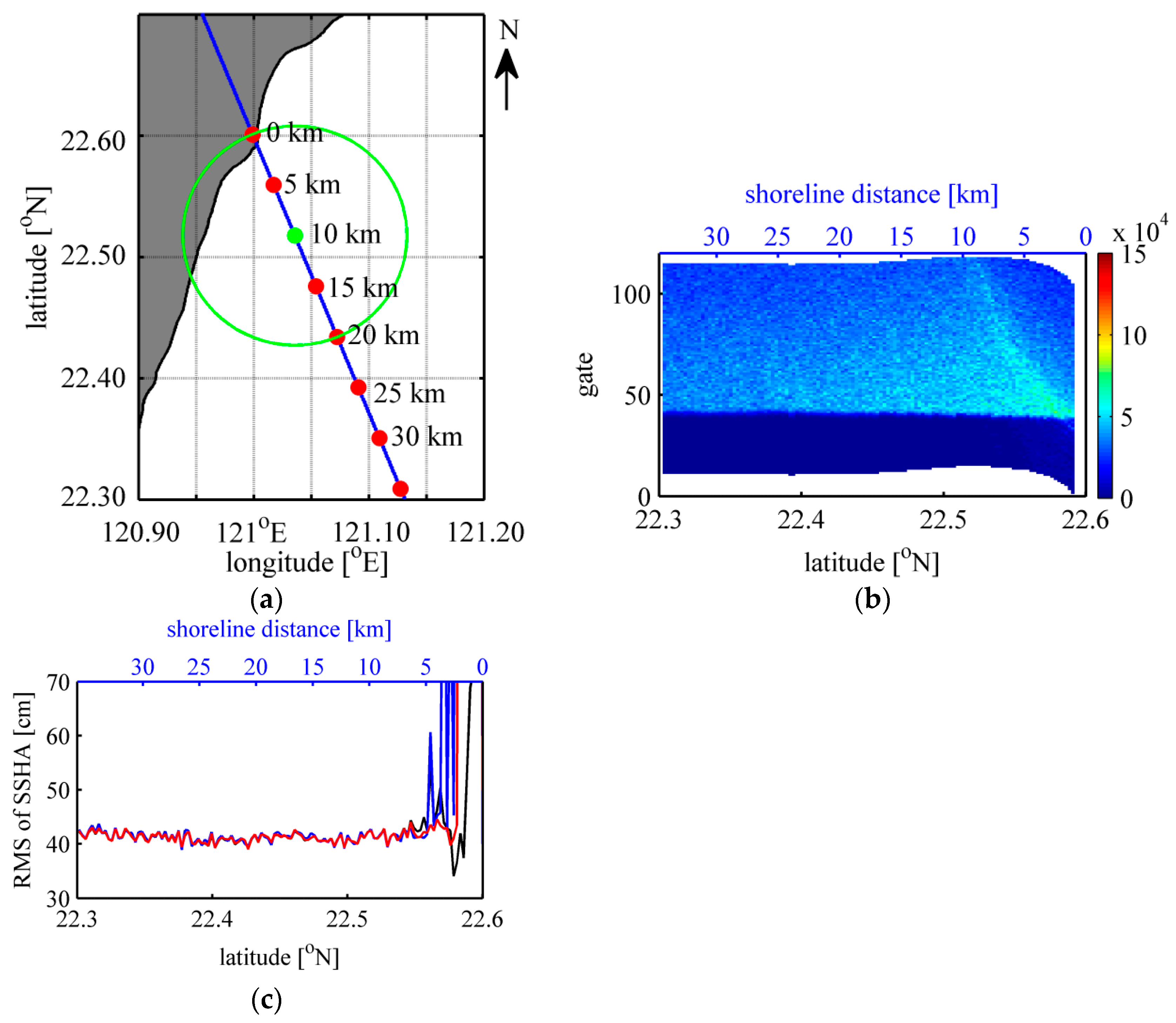
For comparison purposes, retracking for another pass over a relatively smooth coastline is examined. Figure 13a shows pass 164 over the southeast of Taiwan. An example of the along-track echogram (Figure 13b) includes no obvious bright targets. As shown in Figure 13c, the difference among the three retrackers is almost negligible, although the ALES retracker shows a relatively larger RMS within 5 km from the coast.
Overall, the present method enables proper SSHA retrieval even in areas within 10 km from land. Although the approach distance towards the land varies with the geography of the study area, a closer approach is expected using the present method than using the other retrackers. The present method works especially well for removing isolated bright targets, but other factors causing inhomogeneous sea surface reflection, such as internal waves, sigma0 bloom events, and rain cells [17], are currently not considered. Hence, further studies in other coastal zones will be necessary to generalize the efficiency of the present method.
Acknowledgments
The present study was supported in part by a project called “Monitoring and prediction of marine and atmospheric environmental changes in the East Asia” of the Research Institute of Applied Mechanics (RIAM), Kyushu University, and by The Japan Society for the Promotion of Science (JSPS) KAKENHI Grant Number JP15H05821.
Author Contributions
Xifeng Wang contributed to the conception of the study, performed the data analyses, and wrote the manuscript under Kaoru Ichikawa’s guidance. This work was completed in Kyushu University, Japan, when Xifeng Wang was a Ph.D. student.
Conflicts of Interest
The authors declare no conflict of interest.
References
- Chelton, D.B.; Walsh, E.J.; Macarthur, J.L. Pulse compression and sea level tracking in satellite altimetry. J. Atmos. Ocean. Technol. 1989, 6, 407–438. [Google Scholar] [CrossRef]
- Brown, G. The average impulse response of a rough surface and its applications. IEEE Trans. Antennas Propag. 1977, 25, 67–74. [Google Scholar] [CrossRef]
- Hayne, G.S. Radar altimeter mean return waveforms from near-normal-incidence Ocean surface scattering. IEEE Trans. Antennas Propag. 1980, 28, 687–692. [Google Scholar] [CrossRef]
- Tournadre, J. Determination of rain cell characteristics from the analysis of TOPEX altimeter echo waveforms. J. Atmos. Ocean. Technol. 1998, 15, 387–406. [Google Scholar] [CrossRef]
- Tournadre, J. Signature of lighthouses, ships, and small islands in altimeter waveforms. J. Atmos. Ocean. Technol. 2007, 24, 1143–1149. [Google Scholar] [CrossRef]
- Gomez-Enri, J.; Vignudelli, S.; Quartly, G.D.; Gommenginger, C.P.; Cipollini, P.; Challenor, P.G.; Benveniste, J. Modeling Envisat RA-2 waveforms in the coastal zone: Case study of calm water contamination. IEEE J. Geosci. Remote Sens. Lett. 2010, 7, 474–478. [Google Scholar] [CrossRef] [Green Version]
- Gommenginger, C.; Thibaut, P.; Fenoglio-Marc, L.; Quartly, G.; Deng, X.; Gomez-Enri, J.; Challenor, P.; Gao, Y. Retracking Altimeter Waveforms Near the Coasts. A Review of Retracking Methods and Some Applications to Coastal Waveforms. In Coastal Altimetry; Springer: Berlin, Germany, 2011; pp. 61–75. [Google Scholar]
- Hwang, C.; Guo, J.Y.; Deng, X.L.; Hsu, H.Y.; Liu, Y.T. Coastal gravity anomalies from retracked Geosat/GM altimetry: Improvements, limitation and the role of airborne gravity data. J. Geod. 2006, 80, 204–216. [Google Scholar] [CrossRef]
- Bao, L.; Lu, Y.; Wang, Y. Improved retracking algorithm for oceanic altimeter waveforms. Prog. Nat. Sci. 2009, 19, 195–203. [Google Scholar] [CrossRef]
- Passaro, M.; Cipollini, P.; Vignudeli, S.; Quartly, G.D.; Snaith, H.M. ALES: A multi-mission adaptive subwaveform retracter for coastal and open ocean altimetry. Remote Sens. Environ. 2014, 145, 173–189. [Google Scholar] [CrossRef] [Green Version]
- Idris, N.; Deng, X.L. The retracking technique on multi-peak and quasi-specular waveforms for Jason-1 and Jason-2 missions near the coast. Mar. Geod. 2012, 35, 217–237. [Google Scholar] [CrossRef]
- Tseng, K.H.; Shum, C.K.; Yi, Y.; Emery, W.J. The improved retrieval of coastal sea surface heights by retracking modified radar altimetry waveforms. IEEE Trans. Geosci. Remote Sens. 2014, 52, 991–1001. [Google Scholar] [CrossRef]
- Wessel, P.; Smith, W.H.F. A Global Self-consistent, Hierarchical, High-resolution Shoreline Database. J. Geophys. Res. 1996, 101, 8741–8743. [Google Scholar] [CrossRef]
- Thibaut, P.; Ferreira, F.; Femenias, P. Sigma0 blooms in the Envisat radar altimeter data. In Proceedings of the Envisat Symposium, Montreux, Switzerland, 23–27 April 2007. [Google Scholar]
- Fu, L.L.; Cazenave, A. Satellite Altimetry and Earth Science; Academic Press: Cambridge, MA, USA; pp. 11–14.
- Fenoglio-Marc, L.; Fehlau, M.; Ferri, L.; Becker, M.; Gao, Y.; Vignudelli, S. Coatal sea surface heights from improved altimeter data in the Mediterranean Sea. In Gravity, Geoid and Earth Observation; Springer: Berlin, Germany, 2010; Volume 135, pp. 253–261. [Google Scholar]
- Quartly, G.D. Optimizing σ0 information from the Jason-2 altimeter. IEEE Geosci. Remote Sens. Lett. 2009, 6, 398–402. [Google Scholar] [CrossRef] [Green Version]
Figure 1.
Characteristics of a typical Brown waveform over the open ocean.
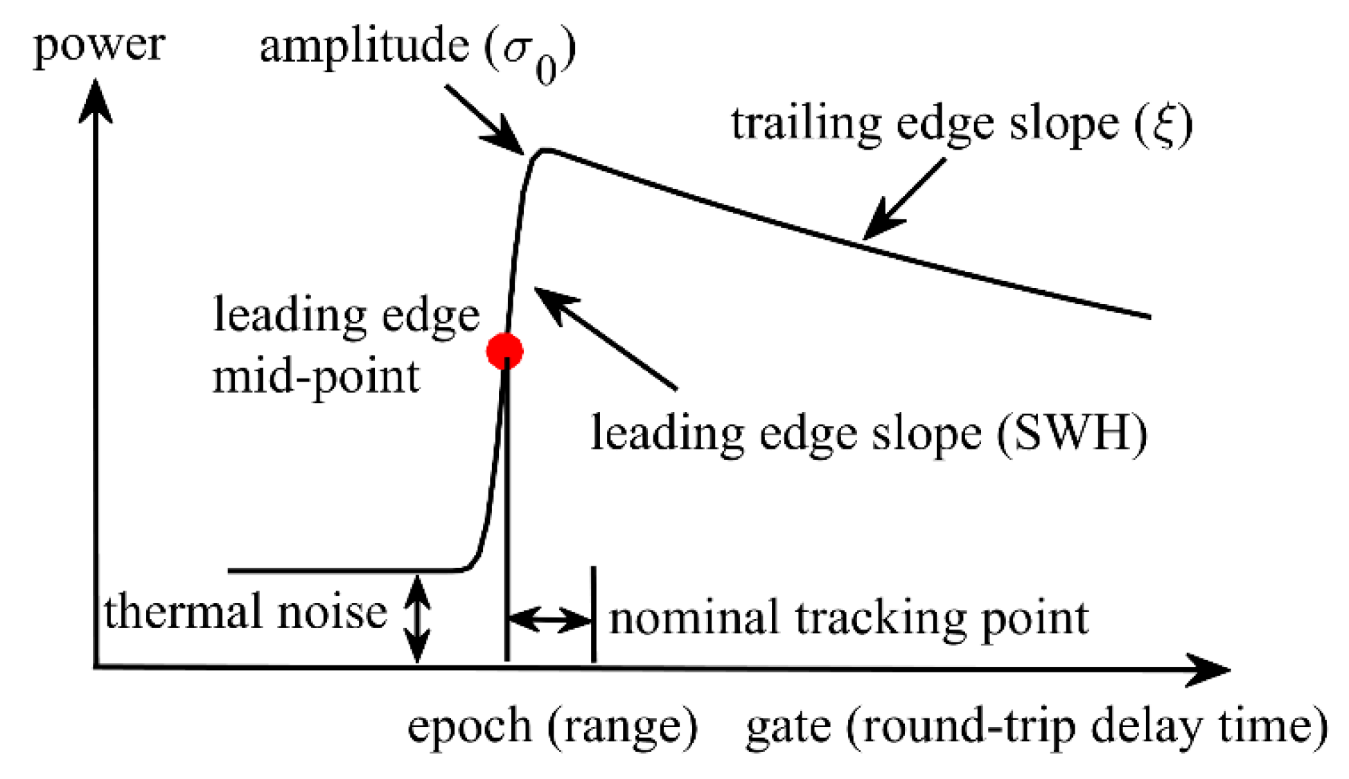
Figure 2.
(a) Rescaled and realigned along-track waveforms (echogram) measured by the Jason-2 altimeter over the southern Tsushima Islands (pass 36, cycle 22). The shaded area (black patch) corresponds to land. Each column of the echogram represents an individual waveform at a given latitude and the rescaled power is indicated by the color scale; (b) Example of corrupted waveform measured at the location indicated by the red point in Figure 2a (34.20°N). The black line represents the actual waveform and red line represents the fitted waveform using the four parameter Brown theoretical model.

Figure 3.
(a) Ground track (blue line) and footprint (blue circles draw for every 1 s, radius is 10 km) of the Jason-2 altimeter over the Tsushima Islands (pass 36). The shortest distance between the tide gauge (red point) and altimeter ground track is about 6 km; (b) Enlarged local map for the southern section of the pass. The vertices in Figure 2a indicate that the reflection points are located 3 km and 5 km apart from the nadir track at 34.23°N and 34.21°N, respectively. These locations, which include semi-closed bays, are marked by circles.
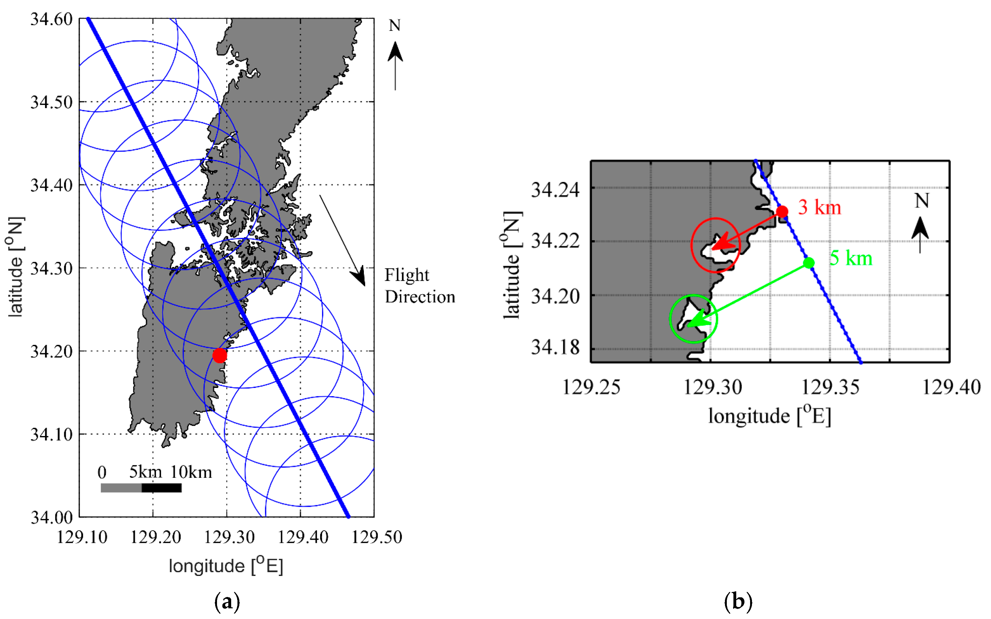
Figure 4.
(a) Schematic showing the geometrical relationship between an altimeter and a strong reflector (bright patch) on the sea surface. The altimeter is closest to the reflector at point with a distance ; (b) Parabolic shape in the echogram. The value corresponds to the geographical distance between point of the altimeter with (nearest approach), and represents the round-trip time difference, .
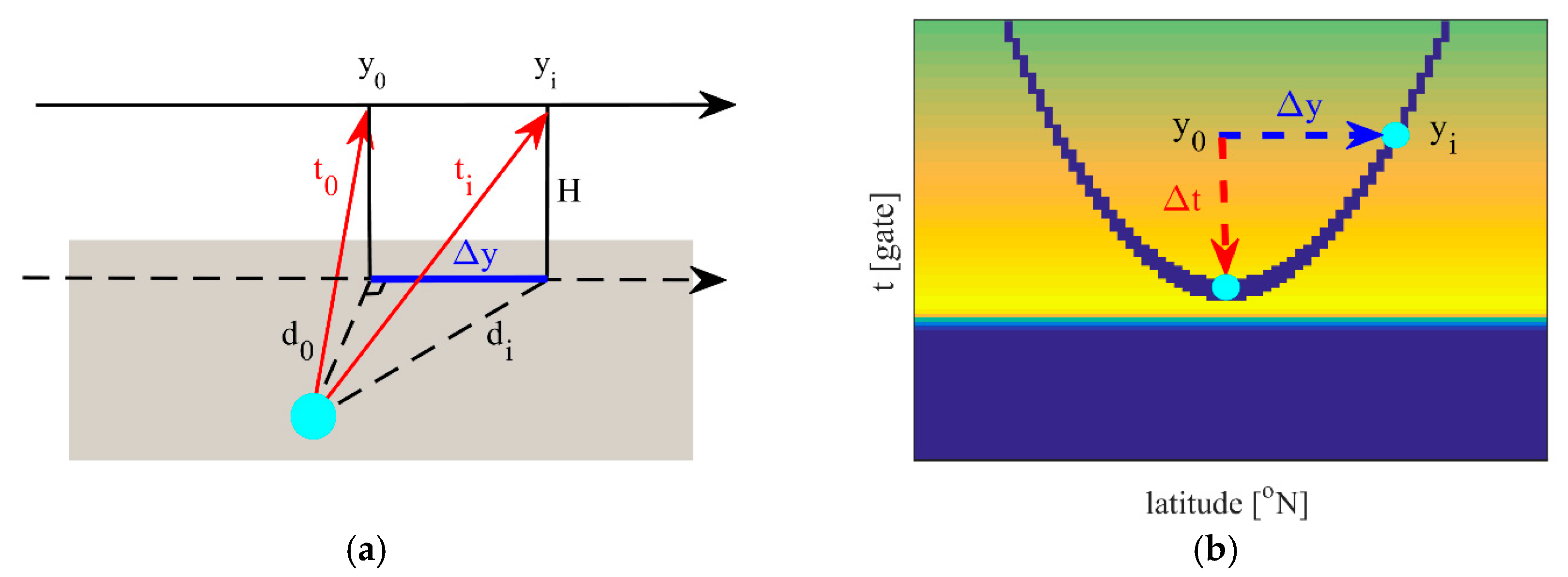
Figure 5.
Purple points represent the marked pixels in the echogram for the 2% threshold criterion. Cyan points represent the parabolic shape described by Equation (2). The red point is the vertex of the parabola.
Figure 5.
Purple points represent the marked pixels in the echogram for the 2% threshold criterion. Cyan points represent the parabolic shape described by Equation (2). The red point is the vertex of the parabola.

Figure 6.
(a) Masked echogram for pass 36 cycle 22 of Jason-2 data south of the Tsushima Islands. All pixel traces along the parabolic shape are masked. The shaded area represents the land; (b) Bright targets masked waveform (dash line) and fitted Brown waveform (solid line) measured at 34.2°N (the same waveform as shown in Figure 2b).

Figure 7.
(a) Annular altimeter footprint (drawn for every five gates) for the waveform measured at 34.2°N (corresponding to the red point shown in Figure 2a); (b) Compensated waveform (dashed line) and the fitted Brown waveform (solid line) measured at the location shown in (a).
Figure 7.
(a) Annular altimeter footprint (drawn for every five gates) for the waveform measured at 34.2°N (corresponding to the red point shown in Figure 2a); (b) Compensated waveform (dashed line) and the fitted Brown waveform (solid line) measured at the location shown in (a).

Figure 8.
SSH (a); SWH (b); sigma0 (c) and mispointing angle (d) before (green) and after (red) land compensation south of the Tsushima Islands for cycle 22 of the Jason-2 altimeter.
Figure 8.
SSH (a); SWH (b); sigma0 (c) and mispointing angle (d) before (green) and after (red) land compensation south of the Tsushima Islands for cycle 22 of the Jason-2 altimeter.
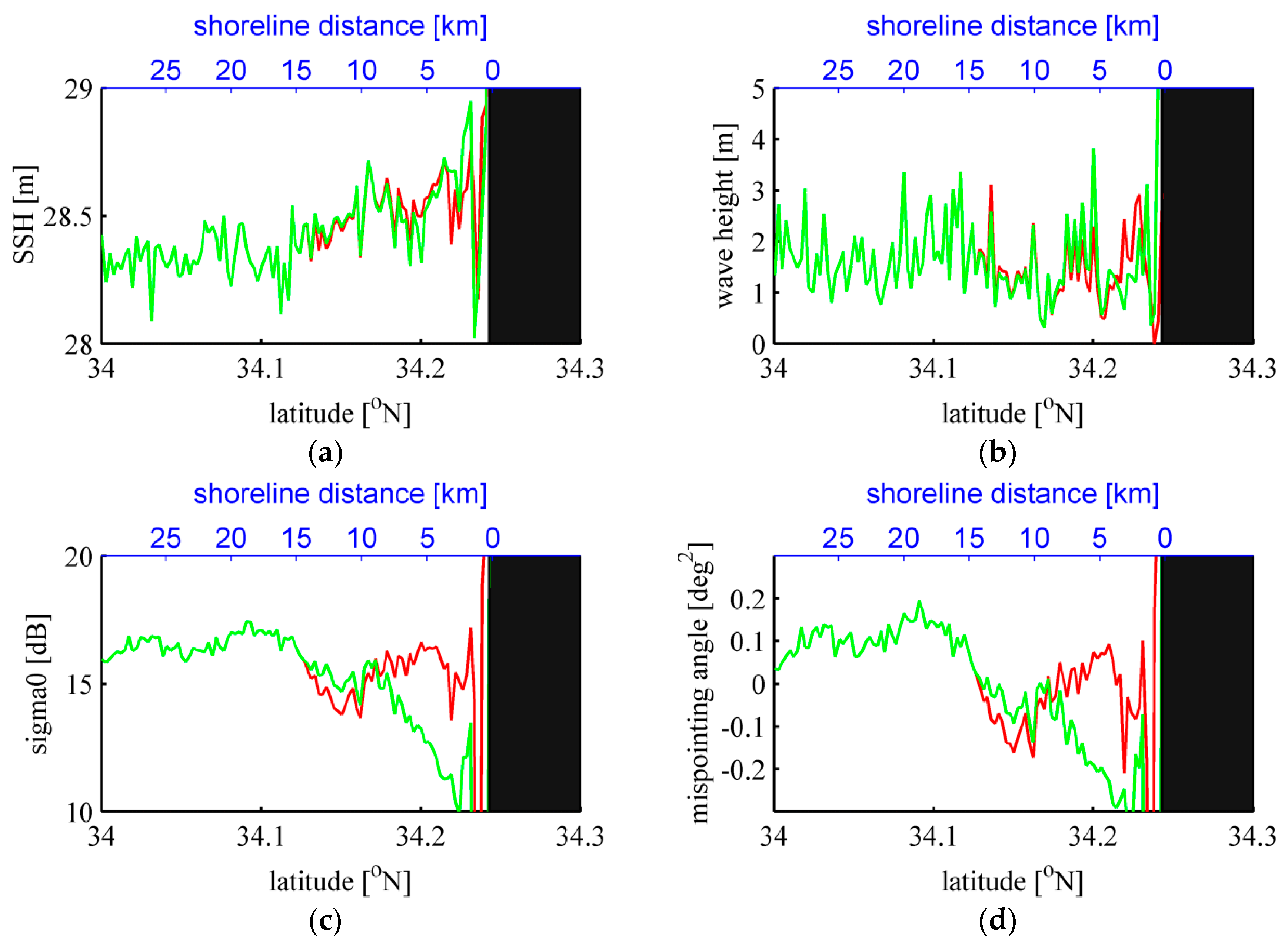
Figure 9.
RMSD between the results with and without land compensation south of the Tsushima Islands for seven years of Jason-2 altimeter data; for range (a); SWH (b); sigma0 (c) and mispointing angle (d).
Figure 9.
RMSD between the results with and without land compensation south of the Tsushima Islands for seven years of Jason-2 altimeter data; for range (a); SWH (b); sigma0 (c) and mispointing angle (d).

Figure 10.
Correlation coefficient (CC) (a) and RMSD (b) for the SSHA derived from tide gauge and altimeter measurements for three different methods. Black is the result for the SGDR product, blue is the result for the ALES product, and red is the result for this study.
Figure 10.
Correlation coefficient (CC) (a) and RMSD (b) for the SSHA derived from tide gauge and altimeter measurements for three different methods. Black is the result for the SGDR product, blue is the result for the ALES product, and red is the result for this study.

Figure 11.
Comparison of SSHA time series derived from ALES retracker (blue) and this study (red) at 34.21°N with tide gauge measurements (green).
Figure 11.
Comparison of SSHA time series derived from ALES retracker (blue) and this study (red) at 34.21°N with tide gauge measurements (green).

Figure 12.
(a) Ground track (blue line) of Jason-2 altimeter pass 36 over northwestern coast of the Tsushima Islands. Points are plotted every 5 km from the coast of Cape Karasaki together with corresponding footprints with a 10 km radius. The section of the pass over Asou Bay is identified by the purple line; (b) Rescaled and realigned along-track waveforms (echogram) measured by the Jason-2 altimeter over the northwestern coast of the Tsushima Islands (pass 36, cycle 22); (c) RMS variation for SSHA derived from altimeter measurements for three different methods. Black is the result of SGDR product, blue is the result of ALES product, and red is the result of this study.
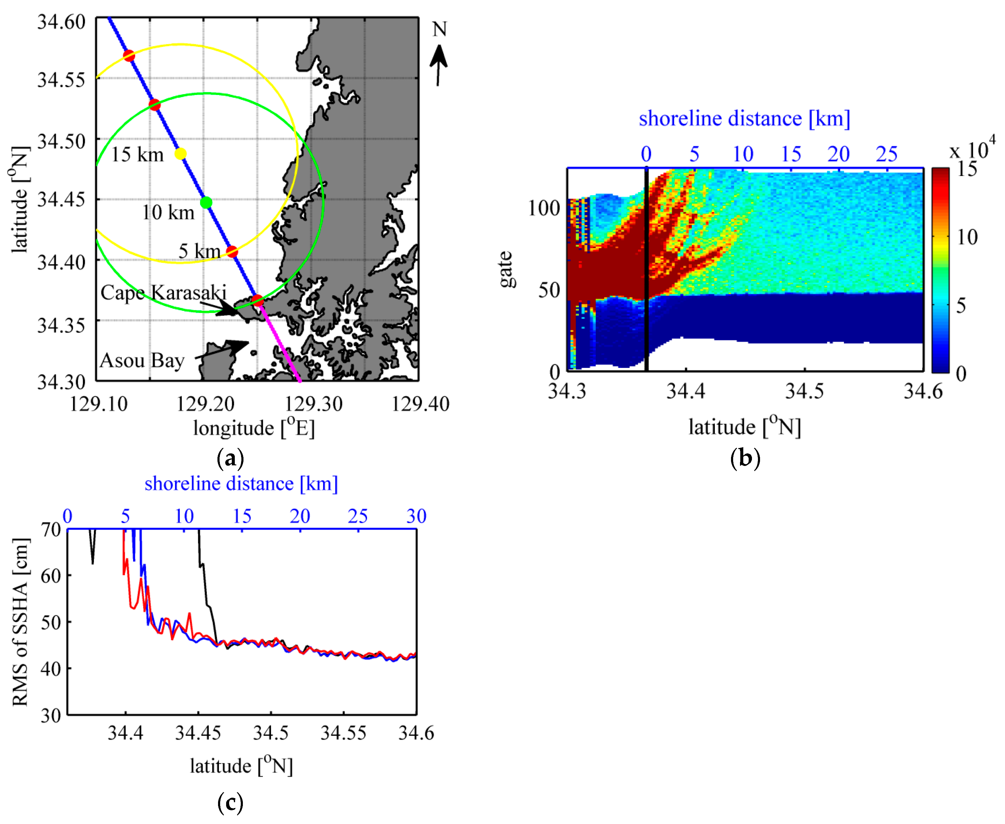
Figure 13.
(a) Ground track (blue line) of Jason-2 altimeter pass 164 over southeast coast of Taiwan. Points are plotted for every 5 km from the coast together with corresponding footprints with 10 km radius; (b) Rescaled and realigned along-track waveforms (echogram) measured by Jason-2 altimeter over Taiwan (pass 164, cycle 47); (c) RMS variation for SSHA derived from altimeter measurements for three different methods. Black is the result for the SGDR product, blue is the result for the ALES product, and red is the result for this study.

© 2017 by the authors. Licensee MDPI, Basel, Switzerland. This article is an open access article distributed under the terms and conditions of the Creative Commons Attribution (CC BY) license (http://creativecommons.org/licenses/by/4.0/).
Share and Cite
MDPI and ACS Style
Wang, X.; Ichikawa, K. Coastal Waveform Retracking for Jason-2 Altimeter Data Based on Along-Track Echograms around the Tsushima Islands in Japan. Remote Sens. 2017, 9, 762. https://doi.org/10.3390/rs9070762
AMA Style
Wang X, Ichikawa K. Coastal Waveform Retracking for Jason-2 Altimeter Data Based on Along-Track Echograms around the Tsushima Islands in Japan. Remote Sensing. 2017; 9(7):762. https://doi.org/10.3390/rs9070762
Chicago/Turabian StyleWang, Xifeng, and Kaoru Ichikawa. 2017. "Coastal Waveform Retracking for Jason-2 Altimeter Data Based on Along-Track Echograms around the Tsushima Islands in Japan" Remote Sensing 9, no. 7: 762. https://doi.org/10.3390/rs9070762
Note that from the first issue of 2016, this journal uses article numbers instead of page numbers. See further details here.