Performance Evaluation for China’s Planned CO2-IPDA
by
 , , ,
, , ,
Ge Han
1 ,
,
Xin Ma
2,*,
Ailin Liang
3,
Tianhao Zhang
3,
Yannan Zhao
4,
Miao Zhang
5 and
Wei Gong
3,* 1
International School of Software, Wuhan University, Wuhan 430079, China
2
Electronic Information School, Wuhan University, Wuhan 430079, China
3
State Key Laboratory of Information Engineering in Surveying, Mapping and Remote Sensing, Wuhan University, Wuhan 430079, China
4
Key Laboratory of Earthquake Geodesy, Institute of Seismology, China Earthquake Administration, Wuhan 430071, China
5
School of Environmental Science and Tourism, Nanyang Normal University, Wolong Road 1638, Nan Yang 473061, China
*
Authors to whom correspondence should be addressed.
Remote Sens. 2017, 9(8), 768; https://doi.org/10.3390/rs9080768
Submission received: 15 June 2017
/
Revised: 21 July 2017
/
Accepted: 21 July 2017
/
Published: 26 July 2017
(This article belongs to the Special Issue Remote Sensing of Greenhouse Gases)
Abstract
:Active remote sensing of atmospheric XCO2 has several advantages over existing passive remote sensors, including global coverage, a smaller footprint, improved penetration of aerosols, and night observation capabilities. China is planning to launch a multi-functional atmospheric observation satellite equipped with a CO2-IPDA (integrated path differential absorption Lidar) to measure columnar concentrations of atmospheric CO2 globally. As space and power are limited on the satellite, compromises have been made to accommodate other passive sensors. In this study, we evaluated the sensitivity of the system’s retrieval accuracy and precision to some critical parameters to determine whether the current configuration is adequate to obtain the desired results and whether any further compromises are possible. We then mapped the distribution of random errors across China and surrounding regions using pseudo-observations to explore the performance of the planned CO2-IPDA over these regions. We found that random errors of less than 0.3% can be expected for most regions of our study area, which will allow the provision of valuable data that will help researchers gain a deeper insight into carbon cycle processes and accurately estimate carbon uptake and emissions. However, in the areas where major anthropogenic carbon sources are located, and in coastal seas, random errors as high as 0.5% are predicted. This is predominantly due to the high concentrations of aerosols, which cause serious attenuation of returned signals. Novel retrieving methods must, therefore, be developed in the future to suppress interference from low surface reflectance and high aerosol loading.
1. Introduction
Recent studies show that half of the predicted anthropogenic CO2 is missing for unknown reasons, resulting in a high level of uncertainty in carbon partitioning models [1,2]. Therefore, detailed observations of surface and columnar CO2 concentrations are urgently required to provide better constraints for atmospheric inversions of carbon sinks and sources [3,4]. Since 2000, several instruments and satellites that use passive remote sensing techniques to retrieve CO2 concentrations have been sent into orbit, including the Atmospheric Infrared Sounder (AIRS), Scanning Imaging Absorption Spectrometer for Atmospheric Chartography (SCIAMACHY), IASI, Greenhouse Gases Observing Satellite (GOSAT), Orbiting Carbon Observatory-2 (OCO-2), and TanSat. Data acquired by these pioneer satellites have deepened our understanding of the carbon cycle despite their susceptibility to sources of bias and insufficient coverage over high-latitude zones [5,6,7,8,9]. In the last decade, differential absorption lidar (DIAL) has shown significant promise in atmospheric CO2 sensing owing to remarkable developments in both the lasers and detectors [10]. Integrated path differential absorption lidar (IPDA), a special type of DIAL, can measure CO2 concentrations with a high precision and improved coverage, and has been widely adopted by several research groups as a next-generation CO2 sensor [10,11,12,13,14]. In recent years, airborne CO2-IPDAs have been extensively tested by different research groups funded by the National Aeronautics and Space Administration (NASA) [15,16,17,18,19,20,21]. In these experiments, researchers have claimed to observe ideal results (i.e., results with random errors below 1%) and are anticipating the realization of space-based CO2-IPDA in the near future. In 2008, researchers funded by the European Space Agency (ESA) published a report in which concepts, objectives, and requirements for a space-based CO2-IPDA were clarified for the first time [22]. In the same year, Ehret et al. carried out a sensitivity analysis to illuminate the specific parameter requirements for hardware (e.g., the laser, detector, telescope) [23]. Kawa et al. conducted a simulation study on the Active Sensing of CO2 Emissions over Nights, Days and Seasons (ASCENDS) [24]. Additionally, similar studies have reported results for space-based methane lidar missions [25,26]. These studies have laid a good theoretical basis for the development of satellite-borne CO2-IPDA and indicate a promising future for active remote sensing of greenhouse gas concentrations.
Following the Unite States and other developed countries, China is interested in developing its own CO2-DIAL or IPDA. A space-based CO2-IPDA has been developed to the demonstration stage in China. Unlike NASA’s program, which placed different sensors on different satellites and realized near- simultaneous observations of a wide variety of parameters through a coordinated group of satellites (A-train) [27], China’s program plans to place multiple sensors, including a CO2-IPDA, a Mie-LIDAR, a wide imaging spectrometer, a multi-angle polarization imager, and a polarization scanner, on a single satellite. This configuration will undoubtedly enhance the consistency of the observations from different sensors, but also will pose greater challenges, such as the allocation of power and space, in their design. The satellite orbit and transit time are set at 705 km and 1:00 a.m./1:00 p.m. Local Standard Time (LST), respectively, to provide similar conditions to other passive sensors; this differs from the orbit and time used by ASCENDS (450 km, 6:00 a.m./6:00 p.m. LST). This type of design will have a negative impact on the signal-to-noise ratio of the IPDA load. We need to quantitatively determine the extent to which these parameter settings will impact the accuracy of CO2 concentration retrievals. Moreover, China’s space-based CO2-IPDA gives priority to atmospheric CO2 detection in China and surrounding regions. The notorious air pollution problems in China will pose a unique and serious challenge for the performance of the space-based CO2-IPDA [28,29]. However, previous studies have paid little attention to performance evaluations under high aerosol load conditions [23,24]. Finally, two important problems should be resolved before production of the final CO2-IPDA product for China. One is whether the current parameter configuration can meet the requirements of high-accuracy atmospheric CO2 detection, and the other is whether there is room to relax the requirements for some parameters without significantly degrading the performance of the CO2-IPDA, thereby reducing its power consumption and space requirements.
To investigate these problems, we studied the effect of the orbit height and solar radiation on the performance of the satellite-borne CO2-IPDA, whose parameters were set according to the current Chinese design. The combined effect of surface reflectance and aerosol optical depth (AOD) on the relative random error was also discussed, and based on this, the existing instrument parameters were optimized using a sensitivity analysis. Finally, real surface reflectance and AOD data for China and surrounding regions were obtained using processed MODIS (Moderate resolution Imaging Spectroradiometer) products to evaluate the performance of the CO2-IPDA and discuss the usability of its products. When mapping the spatial distribution of the relative random errors, we focused our performance evaluation on land areas because the reflectance of oceans is fairly homogeneous. This paper is organized as follows: the calculation methods for the errors, data sources, and the parameter configuration are presented in Section 2; results of the sensitivity analysis for the orbit height, solar radiance, surface reflectance, and AOD are shown in Section 3 alongside the parameter optimization for China’s CO2-IPDA. Section 3 also discusses the performance of China’s IPDA based on maps of relative errors generated using real annual reflectance and AOD products. Finally, we summarize the significant results of this study and present our conclusions in Section 4.
2. Materials and Methods
In this study, three parameters were initially considered for the performance evaluation of the CO2-IPDA: the systemic error, random error, and spatial coverage. The major product of CO2-IPDA is XCO2. However, the XCO2 data provided by this product is subsequently used to invert carbon fluxes to reveal the spatial-temporal distribution of carbon sinks and sources. Errors that vary geographically would be detrimental for these inversions. Additionally, the coverage of XCO2 determines where scientists can retrieve reliable carbon fluxes. In general, the systematic error remains constant globally. Moreover, systematic errors depend strongly on the technological level of the hardware systems. There is almost no correlation between the systematic error and energy consumption or volume occupation of the satellite. Therefore, systematic errors are not a major concern of this work. The coverage could be a critical advantage of IPDA over passive sensors, and is related to orbit height; consequently, this parameter is considered in this study. Finally, random errors are the primary focus of this work because they vary geographically and are strongly related to the design parameters of the CO2-IDPA.
The performance evaluation requires consideration of the interactive relationship between the sensor, environmental, and product models. Hence, all three are involved in this work, as shown in Figure 1. Parameters for the sensor and product models were chosen according to the configuration of China’s planned CO2-IPDA. Parameters for the environmental model were derived from remotely sensed data. In this section, we demonstrate the methodologies used to simulate random errors, systematic errors, and orbit sampling in this work, as well as the values of relevant parameters used in the simulations.
2.1. Random Errors
The total error consists of systematic and random errors. Systematic errors have several sources, but a major proportion is caused by hardware defects, a global and constant bias that has little impact on retrieved CO2 sources and sinks. The remaining proportion fluctuates over various temporal and spatial scales, but is relatively small compared to the constant bias and the random error. Reduction of systematic errors relies on rigid instrument calibration and accurate meteorological parameters, but not on the subsequent processing methods. Random error refers to errors that are highly localized in space and time; these can yield false CO2 sources and sinks. Spatial and temporal averaging can help reduce random errors, meaning that there is a trade-off between resolution and accuracy. Consequently, we will focus on evaluations of the random error in this work.
The random error of XCO2 measurements is equivalent to that of optical depth, owing to the differential absorption effect of CO2, which can be expressed as shown in Equation (1).
where is the optical depth due to absorption of CO2, nshots denotes the number of statistically independent pulse pairs, represents the statistical fluctuation of laser pulse energy measurements, and is the mean signal-to-noise ratio (SNR) of the lidar returns. A typical lidar setup that uses direct detection allows the averaging of a large number of statistically independent speckle cells, satisfying the condition that the mean carrier-to-noise ratio is considerably greater than the speckle-related SNR. Additionally, only two dominant error sources, dark current noise and the solar background noise, are considered herein for simplification. can then be expressed as in Equation (2)
where M is the internal gain factor of the detector, R denotes the responsivity of the detector, B is the electrical bandwidth, e is the elementary charge, F is the excess noise factor of the detector (which accounts for additional noise due to the internal amplification statistics), and is the dark current noise density. is the solar background radiance, which is expressed in Equation (3).
where FOV is the field of view, L is the solar radiance at the top of the atmosphere, A is the effective detection area of the telescope, and Q is the surface reflectance. is expressed in Equation (4).
where D is the total optical efficiency of the CO2-IPDA, O is the overlap function, E is the pulse energy of the transmitted laser radiation, ∆teff is introduced to account for the effective pulse length of the lidar returns and is calculated using Equation (5), is the pulse length, B is the electronic bandwidth, ∆h is the effective target altitude within the footprint of the laser pulse, c is the speed of light, τ is the one-way atmospheric transmission, and rG is the distance between the target and the laser. Further descriptions of relevant parameters, such as molecular spectra, laser line shape, etc., can be found in existing studies [24,29,30] or textbooks [31].
In the following sections, we present sensitivity studies of several key parameters for random errors. Figure 2 shows the importance of these parameters and the method employed to estimate the random errors using the equations shown above.
2.2. Systematic Errors
Referring to studies by Kiemle et al. [25] and Ehret et al. [29], sources of systematic error can be divided into four categories: atmospheric, line parameter, transmitter, and satellite. For a space-borne CO2-IPDA, a constant global bias has no impact on the estimation of carbon sources and sinks, as only the gradients of atmospheric CO2 are relevant [22]. The error derived from the linewidth, a transmitter-related parameter, can be corrected using a gas absorption cell, which is a common part of the frequency stabilization unit [12]. Therefore, this factor will not be discussed further.
Systematic errors are not the focus of this work. Besides, a very detailed evaluation method for the systematic errors of a CO2-IPDA has already been presented by Ehret et al. [29]. Consequently, in this study, we present the evaluation results for systematic errors using the methodology presented in Ehret et al., which is not discussed further. The calculated systematic errors are shown in Table 1.
2.3. Orbit Sampling
At present, the orbit parameters for the CO2-IPDA have not been finalized. The current configuration is very similar to that of the A-train, as shown in Table 2. We investigated the performance of a CO2-IPDA with an orbit altitude of 450 km, which is consistent with the ASCENDS value.
The orbit nadir can be calculated using Equations (6)–(12). The parameters that emerge from these equations are set out in Table 2. In the simulations carried out in this study, the sample density was downscaled to 1% of the original density in the along-track direction to improve the calculation speed. According to the laser parameters shown in Table 2, the repetition frequency is 20 Hz. Hence, is 0.05 s, providing over 50 million samples per month globally, which is a problematically large dataset for subsequent visualization. Consequently, we set to 5 s and the accumulation period to 1 month. It is worth noting that this downscaling process will reduce the number of samples in each track, but will not reduce the number of tracks, so the distribution pattern will remain unchanged.
2.4. Environmental Parameters
In this study, the aerosol products were taken from MODIS. The MODIS Collection 6 (C6) aerosol optical depth (AOD) products, with a 3-km spatial resolution at nadir, were released in 2016, and have generally been shown to achieve the required accuracy, as validated by sun photometer observations from the Aerosol Robotic Network (AERONET) in China. In this study, the AOD products from both MODIS Terra and MODIS Aqua, covering the study region with a spatial resolution of 3 km and spanning the period from November 2015 to October 2016, were downloaded from the NASA Land and Atmospheres Archive and Distribution System (LAADS) website. Using these data, we calculated the yearly average for each pixel. Although there are numerous blank values in the daily product, the combined yearly product covers almost the whole of China and surrounding regions, except for the Taklimakan Desert in northwestern China.
Surface reflectance over land areas was obtained using the MODIS (Terra/Aqua) 5 km, 16 d composite bidirectional reflectance distribution function (BRDF)-adjusted data at band 6 (1.64 μm). We collected 3 products on the 5th, 15th, and 25th of each month because the temporal variation in the surface reflectance is small. The yearly product was then calculated by averaging. There are no blank values in our study area. For the reflectance over oceans, a constant value of 0.05 was used because this parameter was relatively homogenous and this study predominantly focuses on land areas.
Image registration was carried out for the reflectance and AOD products to generate spatially and temporally consistent input datasets for further analysis.
2.5. CO2-IDPA Configuration
Table 3 lists the parameters used in the simulation in this study. The load-related parameters are consistent with those of China’s CO2-IPDA, which is under development at the Shanghai Institute of Optics and Fine Mechanics, the Chinese Academy of Sciences. The default values of reflectance and AOD are also presented here. In the experiments described below, we analyzed the model’s sensitivity to different parameters separately. Each subsection below describes the variation of one target parameter. Settings for other parameters are as given in Table 3. In the experiment described in Section 3.4, the default values of reflectance and AOD were replaced by measurements to provide a more realistic simulation. Moreover, the horizontal resolutions of the retrievals over land and over ocean are different, as shown in Table 3.
3. Results
3.1. Critical Orbit Parameters
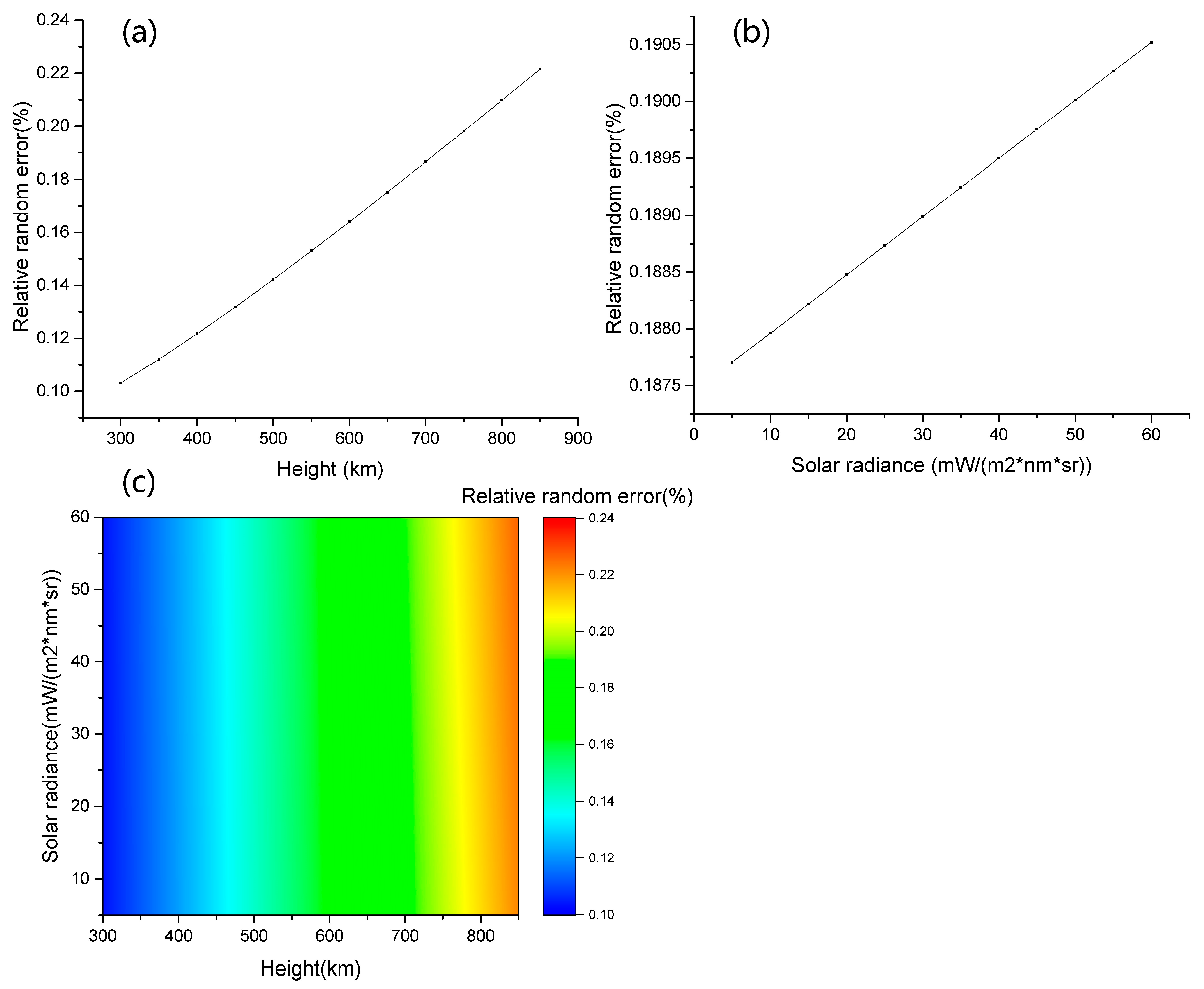
Among all the orbit-related parameters, the orbit altitude and solar radiation were identified as the critical parameters that differed from those for other space-borne CO2-IPDAs. To improve the performance of other passive sensors, the transit time of the satellite was set to noon and the orbit height was set significantly higher than that of the ASCENDS satellite. It is worth noting that there is no relationship between solar radiance and orbit height. Moreover, the relationships between the random errors and the solar radiance, and between the random errors and the orbit height, are linear. In Figure 3, the relative random error is shown to be a function of the solar radiance and orbit height, highlighting the critical orbit parameter. Figure 3 demonstrates the results of the simulation when the solar radiance was set to vary from 5 to 60 mW/(m2 nm sr) and the orbit height from 300 to 850 km. The assumed maximum solar radiation is significantly higher than the most extreme possible case (the mean solar radiation at 1.6 μm is approximately 5 mW/(m2 nm sr)), exaggerating the possible effects of solar radiation. This simplifies the simulation because accurately calculating the solar radiation for given conditions is a complex procedure. Nevertheless, the effect of solar radiation is almost negligible compared to that of the satellite orbit height, according to Figure 3. Compared to the results for a track height of 405 km, results obtained using a value of 700 km showed that the relative random error almost doubled. Fortunately, using an orbit height of 705 km will not result in a relative error exceeding the ideal target as long as other parameters meet or surpass the original hypothesis, as shown in Table 3. We think that the current orbit parameter configuration can fulfill the demand for accurate and precise global XCO2 measurements.
The orbit altitude influences the distribution of samples as well as the influence on the random error. Unlike passive remote sensing of CO2, the IPDA yields a uniform coverage in terms of latitude regardless of the satellite’s altitude. This feature is significant for determining carbon fluxes in high-latitude regions, where the uncertainty of the carbon flux is relatively high because of the insufficient coverage of in-situ and passive remotely sensed measurements. Furthermore, samples from both ascending and descending tracks should provide useful datasets because the IPDA relies on reflected laser signals but not solar signals. In terms of the cloud effect, the cloud fraction should be low for IPDA data compared with passive sensor data, because the diameter of the laser footprint on the ground is 45 m (70.5 m) for a satellite altitude of 450 km (705 km) with a divergence angle of 0.1 mrad. Additionally, the IPDA can utilize reflected signals from thick clouds, particularly low altitude clouds. Therefore, IPDA samples are more useful than those from passive sensors such as GOSAT and OCO-2.
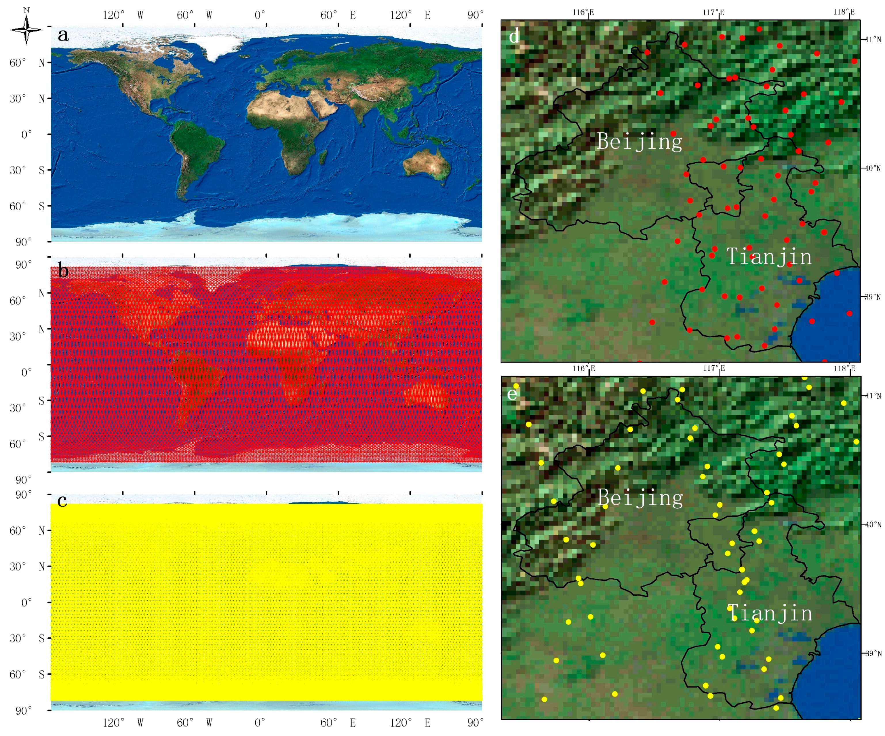
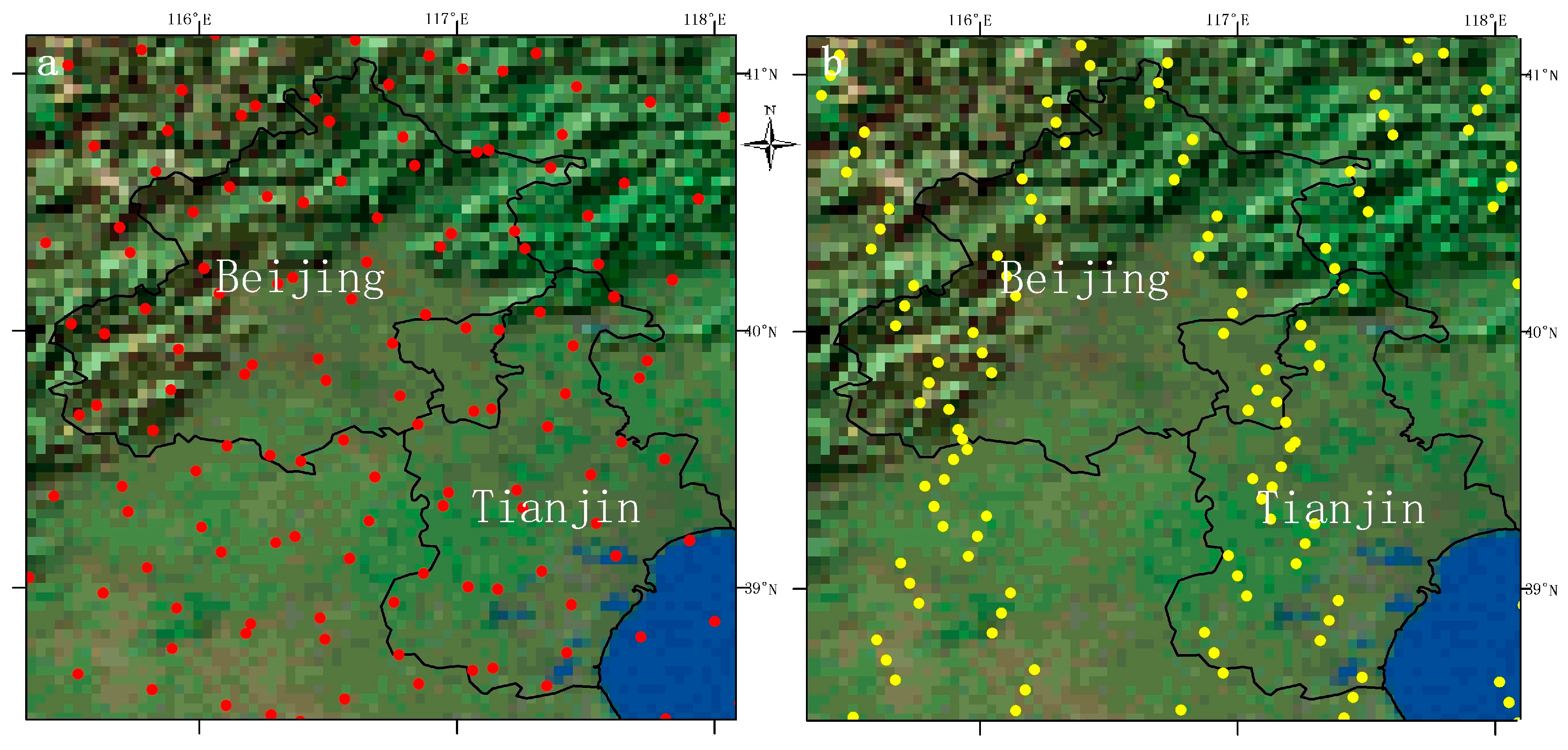
The different settings for the orbit altitude will also influence the distribution of samples, as shown in Figure 4. In this experiment, the observation period was set to one month. Using an orbit altitude of 705 km, samples are more evenly distributes than when using an orbit altitude of 450 km. There are evident gaps in Figure 4b. Therefore, we show a close-up image of the Jing-jin-ji area, where China’s capital and another municipalities are located, to investigate the details of the sample distribution. Figure 4d shows that a group of tracks, taken using an orbit altitude of 450 km, are clustered together to give a high-density sample area. However, there are also large blank areas between different clusters. In contrast, there is no evidence for clusters of tracks when using an orbit altitude of 705 km.
However, a different phenomenon emerges when we expand the observation period, as shown in Figure 5. A uniform distribution pattern of nadir points is acquired using an orbit height of 450 km, as shown in Figure 5a. Using an orbit height of 705 km, there are no evident differences between one-month accumulations and two-month accumulations, as shown in Figure 5b. The number of nadir samples is the same for the two different orbit heights because the laser repetition frequency and the observation period were unchanged. Consequently, more samples were obtained in each track at an orbit height of 705 km.
The differences in the observation period influence the distribution pattern of nadir points because different orbit heights yield different revisit periods (c. 26 days for 705 km and c. 41 days for 450 km). An orbit height of 450 km is therefore a better choice for research based on long-period observations. However, for studies looking to infer monthly CO2 fluxes from global or regional XCO2 measurements from the CO2-IPDA, an orbit height of 705 km might be a better choice.
3.2. Critical Hardware Parameters
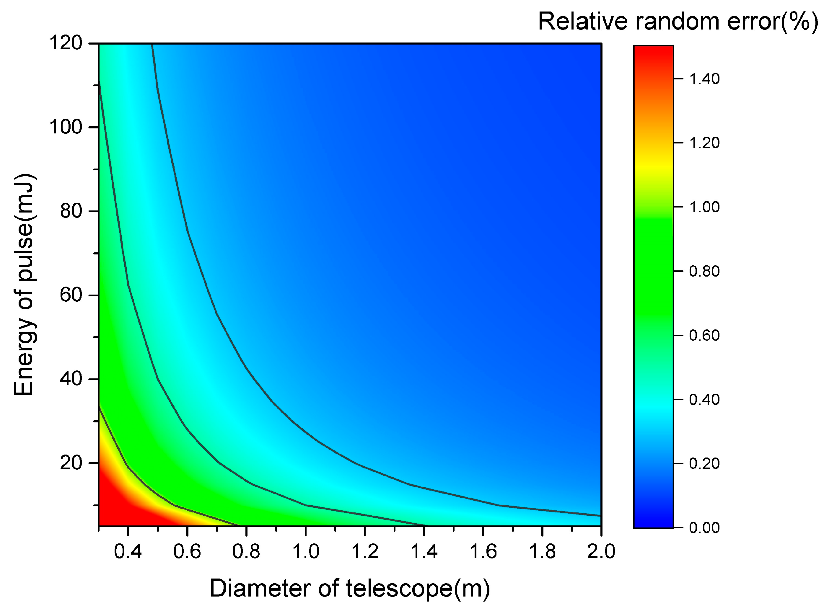
The energy of a single pulse and the laser repetition frequency determine the output photon number per unit time, which eventually determines the SNR of received signals. The repetition frequency was fixed after the laser was developed; consequently, only the pulse energy is considered here. In reality, many other hardware parameters, such as line width, wavelength stability, and the quantum efficiency of detectors, also affect the performance of the CO2-IPDA. However, these parameters do not affect the allocation of satellite resources and are therefore not included in this analysis. The diameter of the telescope is the major determining factor for the volume of the CO2-IPDA load, while the pulse energy determines its power consumption. Three contour lines for the relative error are drawn in Figure 6, representing our ideal target (0.3%), medium target (0.5%), and threshold (1%). Figure 6 shows that pulse energy plays an almost identical role to telescope diameter in determining the relative error. This phenomenon is to be expected because the laser energy determines the total number of photons emitted, while the diameter of the telescope determines the proportion of photons that can arrive at the detector. According to Equations (1)–(3), the relative random error is inversely proportional to E and to the square of diameter. Hence, increasing the diameter has a larger effect than increasing E. However, from an engineering perspective, it is easier to double E than to double the diameter.
Considering the standard diameter of commercially available telescopes, a diameter of 1 m is considered a suitable design. Based on this premise, the corresponding single-pulse energy can be halved compared with the original design, which leaves a margin to reduce energy consumption. The combination of a pulse energy of 75 mJ and a diameter of 1 m would leave sufficient buffer space for the extreme conditions that might be encountered during actual measurements. In conclusion, there is some room for compromise in the design parameters for the pulse energy or telescope diameter.
3.3. Critical Environmental Parameters
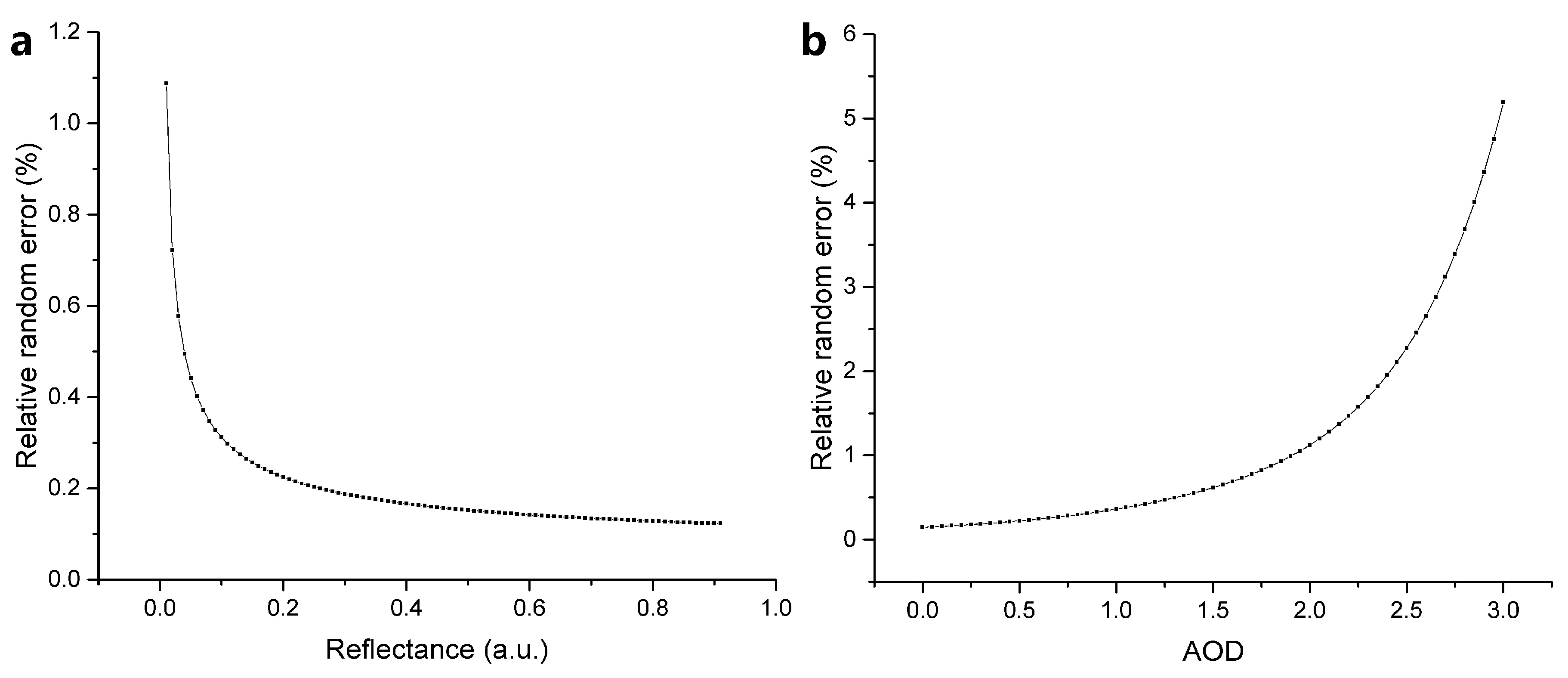
When other conditions remain unchanged, the relationship between each parameter discussed above and the performance of the CO2-IDPA load is linear. Nevertheless, the relationship between critical environmental parameters and the performance of the CO2-IPDA is nonlinear. Referring to Equation (2), the composition of the errors in a single pulse is very complex. When the reflectance is so large that the dark current noise is a relatively small component of the total error, the relative random error is inversely proportional to P, which is linearly related to the reflectance. However, when the dark current noise dominates the total noise, any slight increase in P leads to a significant improvement in the SNR. This explains why the relationship between reflectance and relative random error is not linear.
Regarding reflectance, when the surface reflectance is greater than 0.4, the relative error decreases slowly and almost linearly with increasing reflectance. In contrast, the relative error increases dramatically with decreasing reflectance when the reflectance is lower than 0.15. This relationship could be an obstacle to obtaining accurate and precise measurements with high spatial resolution over seas, where the reflectance is rarely greater than 0.08. Meanwhile, the land surface reflectance varies between 0.1 and 0.6 with respect to different land cover types, implying that the spatial distribution of the performance of the CO2-IPDA may be heterogeneous.
Figure 7 demonstrates accelerating growth in the relative error with increasing AOD. Surprisingly, the increase in the relative error caused by high aerosol loadings overwhelms that caused by low surface reflectance. P is proportional to τ2 and . Hence, P is inversely proportional to the square of AOD. This explains why the effect of AOD is larger than that of reflectance.
Figure 7 explicitly demonstrates that the relative error could easily exceed the threshold of 1%. When AOD is greater than 2, meaningful measurements cannot be acquired by the CO2-IDPA. Taking into account the frequent occurrence of heavy pollution [32] and the high AOD levels [33] in China, it would be a challenging task to retrieve XCO2 accurately over most urban areas.
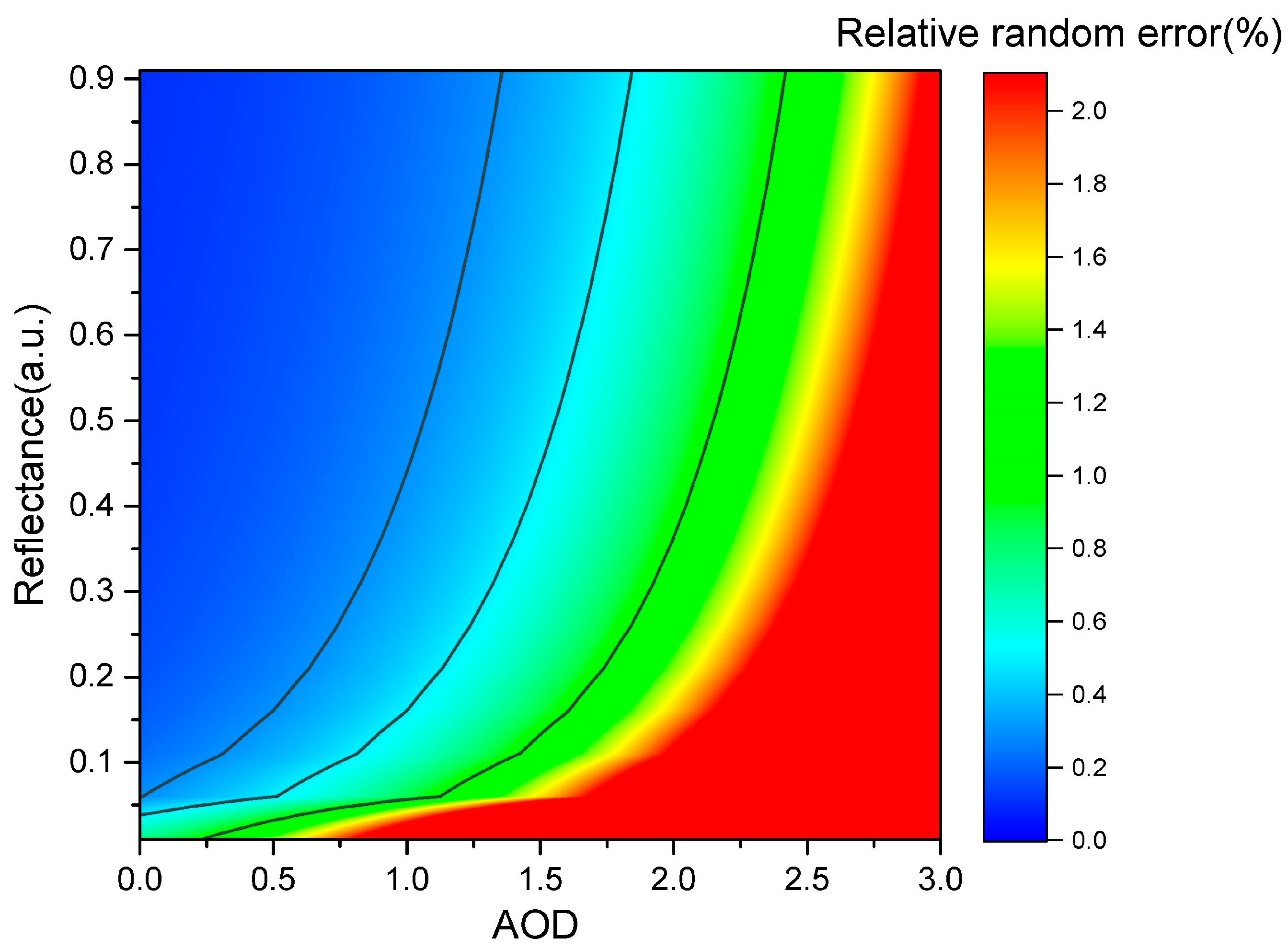
Figure 8 demonstrates the combined effect of two key environmental parameters on the performance of China’s CO2-IDPA. The ideal target cannot be reached in regions where the AOD is greater than 1.3. The reflectance of most human settlements where anthropogenic CO2 is emitted into the atmosphere is lower than 0.35, suggesting that the maximum AOD that allows the ideal performance target to be met may be 0.8, unless further improvements are made to the hardware system or the retrieving algorithm. Ideal results are very likely to be obtained over forests because aerosol loadings are usually low. In desert areas, where the reflectance can reach 0.6, the retrieval threshold will not be exceeded even when AOD > 2, indicating that China’s CO2-IPDA could yield useful results when these regions experience sandstorms. As shown in Figure 7 and Figure 8, environmental parameters seem to play a much more significant role in determining the performance of the CO2-IDPA when the margins for improvement in the hardware and orbital parameters are small. To this end, a detailed simulation will be carried out, supported by real measurements of reflectance and AOD acquired by remote sensing satellites, to explore the performance of China’s CO2-IDPA in China and surrounding regions, and to facilitate finalization of the prototype design.
3.4. Performance Evaluation in China and Surrounding Regions
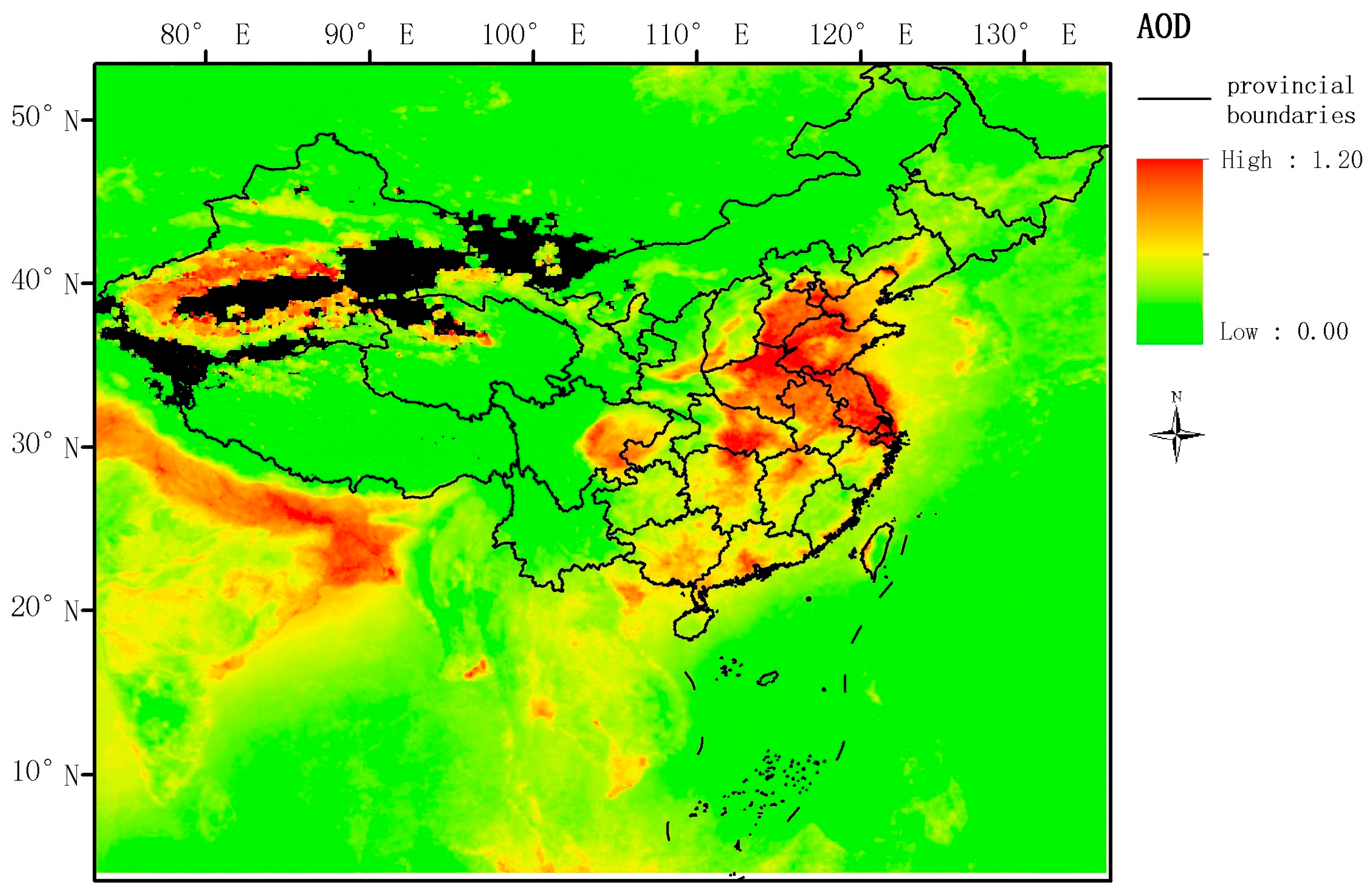
Figure 9 and Figure 10 demonstrate the yearly average AOD and reflectance, respectively. No available AOD data were obtained in Taklimakan Desert for the whole year. This was mainly due to an intrinsic constraint on the commonly used AOD inversion method, known as the dark target method, which applies only to areas with low surface reflectance. Except for desert areas, other areas with high aerosol loadings include almost all the major Chinese cities. Very high pollution levels (AOD > 1.0) were observed in northern, eastern, and central China, the Sichuan Basin, and the Pearl River Delta region. Regarding the reflectance distribution, the surface reflectance is higher in northwestern China and lower in the southeastern region.
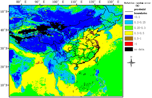
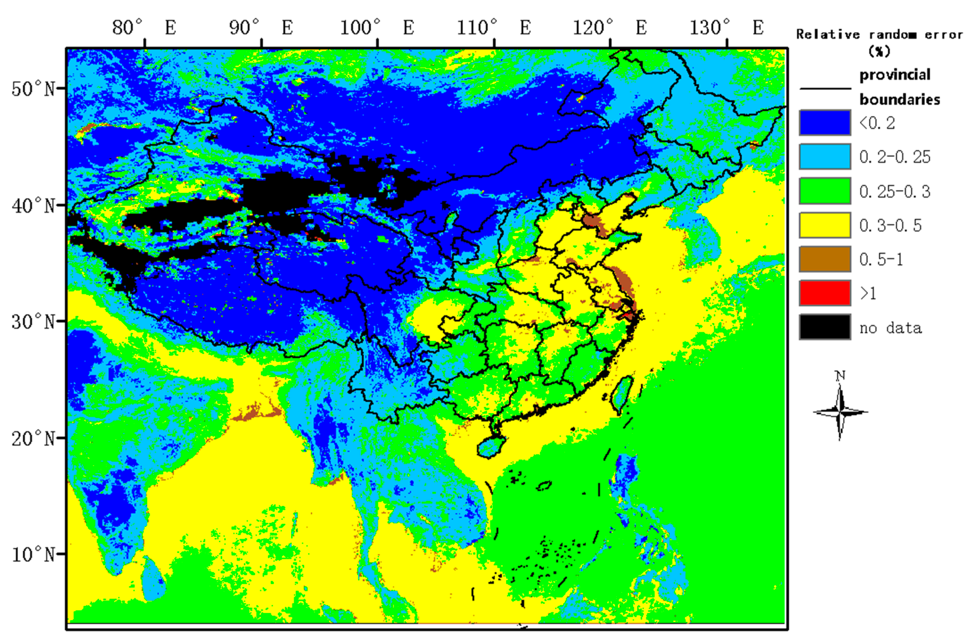
Figure 11 demonstrates the spatial distribution of relative random errors calculated using the methodology described in Section 2 and data presented in Figure 9 and Figure 10. The spatial resolution was set to 50 km over land and 100 km over oceans, and the temporal resolution was set to 16 days. There are blank areas in Figure 11 because of a lack of AOD data. Figure 11 demonstrates that the relative random error is lower in western China compared with eastern China. Moreover, compared with land areas, the relative random error over seas is higher, even though the spatial resolution was downscaled to 100 km. The relative random error can be kept below 0.3% in most of the surrounding areas except for northern India.
4. Discussion
4.1. Comparisons with Passive Sensors
Three satellite-borne CO2 sensors already exist: GOSAT, OCO-2, and TanSat. Additionally, GOSAT-2 is scheduled to be launched in 2018. Consequently, it is necessary to explain why yet another satellite-borne CO2 sensor is needed. Unlike the existing sensors, China’s CO2-IPDA is an active sensor for CO2 measurements. The IPDA has several advantages over passive sensors, such as improved coverage in high-latitude regions, the ability to obtain a greater number of samples over cloudy areas, relatively small systematic errors, and the capability to undertake night measurements. Based on the experiments above, we can now compare the coverage and systematic error of the planned CO2-IPDA with OCO-2, which is currently the best CO2 satellite sensor.
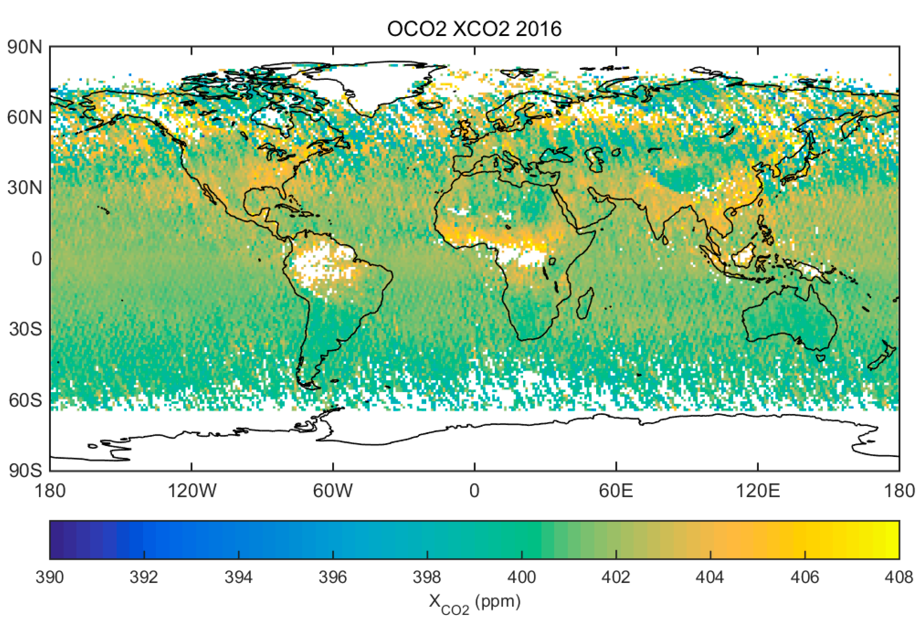
Figure 13 demonstrates the global map of XCO2 from OCO-2 in 2016. Referring to Figure 4, the CO2-IPDA would provide useful supplementary data that could fill the gaps shown in Figure 13. The lack of precise knowledge on carbon sequestration in boreal terrestrial ecosystems imposes a great challenge on the resolution of the mystery of the missing carbon. With the help of CO2-IPDA, XCO2 could be efficiently mapped in high northern high latitudes.
Table 4 demonstrates the validation results for OCO-2. The bias was calculated as the absolute difference between OCO-2 retrievals and Total Carbon Column Observing Network (TCCON) measurements. Because there are no real measurements available for CO2-IPDA, we compared the performance of the CO2-IPDA with that of OCO-2 using theoretical systematic and random errors. The systematic error was compared with the bias while the random error was compared with the Root Mean Square (RMS) error.
Regardless of the version of XCO2 products, both random and systematic errors from CO2-IPDA products were lower than those from OCO-2. Furthermore, quality filters were applied to the XCO2 products used in [31,32] according to Mandrake’s report [35]. The upper limits for AOD_sulfate and AOD_dust are 0.4 and 0.3, respectively. Referring to Figure 7, with an AOD below 0.3, the predicted random error for CO2-IPDA was below 0.3% for nearly all the land areas of China. Consequently, the launch of CO2-IPDA would significantly improve the precision of XCO2 products, especially for areas where the air pollution is too great to obtain useful retrievals using OCO-2.
4.2. Selection of an Appropriate Weighting Function
As well as the precision and sampling coverage, the issue of the weighting function must be addressed. The direct physical quantity provided by CO2-IPDA is the total differential absorption optical depth, not the amount of CO2. Different on-line wavelength selections yield different weighting functions. Because our goal is to map the distribution of carbon sinks and sources, we need retrievals to be sensitive to CO2 in the lower troposphere where emission and uptake of carbon occurs. A weighting function is defined in Equation (13). p and T are atmospheric pressure and temperature, respectively, σ is the absorption cross-section, g is the acceleration due to gravity, and Mair is the average mass of a dry air molecule.
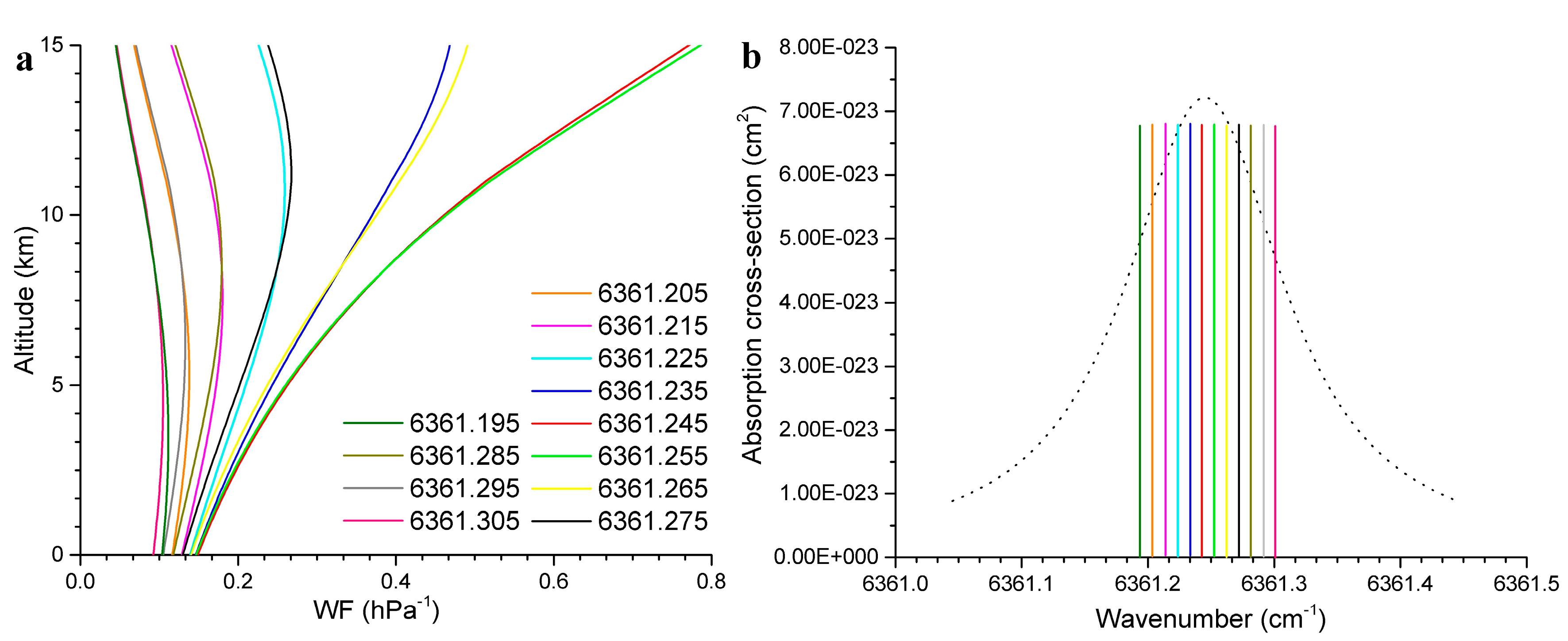
Using the US standard atmosphere model [36] and HITRAN2012 [37], we simulated a weighting function for several candidate on-line wavelengths belonging to line R18 in the 30012←00001 CO2 band.
Figure 14a demonstrates that the central wavenumber is not the best candidate in terms of the WF. 6361.195/6361.305 cm−1 would be very sensitive to the lower troposphere. However, their corresponding differential optical depth would be small according to Figure 14b. As a consequence, the relative error would be enlarged dramatically according to Equation (1). 6361.225 cm−1 is moderately sensitive to the lower and is evidently better than the central wavelength in terms of the WF. Meanwhile, its corresponding differential optical depth is over 0.8. Consequently, 6361.225 cm−1 could represent a good compromise for selection of an on-line wavenumber.
Our previous study showed that selecting an on-line wavenumber in R16 may give lower interference from water vapor [30]. Consequently, a displacement of 0.2 cm−1 from the line center of R16 (i.e., 1.6 μm) probably represents the optimum solution for selection of an on-line wavelength.
4.3. Usage of the Planned CO2-IPDA in China
With its current configuration, the ideal target for China’s CO2-IPDA is predicted to be the majority of mainland China. Some major forested areas, including the Greater Khingan Mountains and Xishuangbanna Tropical Rainforest, are located in this area, suggesting that the launch of the CO2-IPDA could clarify the carbon uptake of China’s major carbon sinks and thus deepen our understanding of the effect of this vegetation on the carbon cycle. Moreover, the CO2-IPDA would provide accurate measurements for the major grasslands in China, including the Hulunbuir Grasslands, Xilin Gol Prairie, Ili Grassland, and Nagqu Alpine Grassland, which will provide precious opportunities to study the inter-annual variations in the grassland characteristics. Based on the performance evaluation from the border of the Taklimakan Desert, inversions for Taklimakan Desert should give relative random errors of no more than 0.5. This could help verify the discovery of a hidden carbon sink in desert regions [38].
However, the accuracy of the measurements for carbon source regions is a concern. Figure 11 shows that the ideal target will not be met for nearly all of China’s cities. Referring to economic data [39], China’s CO2-IPDA will not be able to obtain inversion results with errors of less than 0.3% for the regions responsible for more than 80% of China’s total GDP, which could be problematic for carbon inversions in these areas. We attribute the poor performances of the CO2-IPDA to the large quantities of air pollution present in the urban areas of China. From Figure 9 and Figure 11, a clear correlation is evident between AOD and the relative random error. Hence, we propose that with the current hardware system design and planned orbit, AOD is the most critical factor in determining the accuracy of the inversion results from China’s CO2-IPDA over land areas. A novel retrieval method that suppresses errors derived from high aerosol loadings is urgently needed to solve the anticipated problem in the estimation of China’s carbon emissions using data from the new satellite.
Regarding the remote sensing XCO2 data from sea areas, only the medium goal could be realized for coastal seas, and this would require a decrease in the spatial resolution to 100 km. The relatively low reflectance of water is identified as the primary cause of the low accuracy over seas. It is noteworthy that CO-IPDA’s detection accuracy over China’s Bohai Sea and Yellow Sea will be very limited because of the combined effect of high aerosol concentrations and low reflectance. This disadvantage poses a challenge in estimations of the carbon exchange between land and sea. Over the South China Sea, the ideal target can be met.
In general, China’s CO2-IPAD can achieve useful XCO2 measurements that will facilitate a more accurate determination of carbon fluxes and thus an in-depth understanding of carbon cycle mechanisms. In just 0.031% and 0.705% of areas in China and the surrounding regions, errors will exceed 1% and 0.5%, respectively. The ideal target (i.e., errors below 0.3%) will be met in 74% of regions.
If the orbit height was reduced to 450 km, the situation would be very different. A relative random error of less than 0.2% would be expected for over 75% of regions, and the ideal target could be met in over 95% of regions. This is a very promising outlook. Moreover, in this scenario, an on-line wavenumber that provided better sensitivity to CO2 in the lower troposphere could be selected, because the relative random error would be less than 0.2% in most areas. This error leaved room for the selection of a weighting function that lowers the differential absorption optical depth but increases sensitivity to the lower troposphere. Consequently, we strongly recommend that the planned orbit height for the CO2-IDPA should be reduced.
5. Conclusions
In this study, we analyzed the sensitivity of some critical parameters to the relative random error of China’s CO2-IDPA and evaluated its performance in China and surrounding regions. We found that the satellite transit time does not have a noticeable impact on the relative random error. But the relative random error would be reduced by 0.1% (Noting: the total budget of relative random error is just 0.3%) if the current satellite height was adopted rather than a satellite height of 450 km (ASCENDS’s parameter). Moreover, a high-altitude orbit would lead to obvious gaps between adjacent tracks compared with a low-altitude orbit. The current configuration of the laser, detector, and telescope can yield retrievals of adequate accuracy under normal conditions. However, the high aerosol loadings in China will certainly lead to a significant deterioration in performance. A synthetic simulation based on real measurements of environmental parameters revealed that, using the current configurations of the CO2-IPDA, accurate measurements of XCO2 (random error < 0.3%) look possible for most regions, including the major forests and grasslands in China. However, our study also showed that in the most densely populated regions, the accuracy of XCO2 measurements is unlikely to reach the ideal target (random error < 0.3%). A similar conclusion also holds for the coastal seas. The medium target (random error < 0.5%) can be fulfilled in all the above-mentioned areas. In contrast, passive sensors have failed to carry out successful inversions under similar conditions. However, the development of a novel inversion method for CO2-IPDA is still required to improve its performance to meet the ideal target of 0.3% in those areas where aerosol concentrations are frequently high. Finally, if the orbit height could be reduced to 450 km, the ideal target would be achieved for over 95% of regions.
Acknowledgments
This work was supported by the National Natural Science Foundation of China (Grant No. 41127901 and No. 41601351), a China Postdoctoral Science Foundation funded project (Grant No. 2016M592389 and No. 2017T100580) and the Fundamental Research Funds for the Central Universities (Grant No. 2042016kf0032). The authors wish to thank the Satellite Environment Center, Ministry of Environmental Protection, National Satellite Meteorological Center, China Meteorological Administration and Shanghai Institute of Optics and Fine Mechanics, the Chinese Academy of Sciences for providing the configuration of the CO2-IPDA.
Author Contributions
Ge Han proposed the idea and wrote the manuscript. Xin Ma and Miao Zhang corrected the manuscript and collected necessary data and parameters. Ailin Liang, Tianhao Zhang, and Yannan Zhao conducted experiments. Wei Gong funded this research and negotiated with the cooperators mentioned in the acknowledgments.
Conflicts of Interest
The authors declare no conflict of interest.
References
- Fan, S.; Gloor, M.; Mahlman, J.; Pacala, S.; Sarmiento, J.; Takahashi, T.; Tans, P. A large terrestrial carbon sink in North America implied by atmospheric and oceanic carbon dioxide data and models. Science 1998, 282, 442–446. [Google Scholar] [CrossRef] [PubMed]
- Tans, P.P.; Fung, I.Y.; Takahashi, T. Observational constraints on the global atmospheric CO2 budget. Science 1990, 247, 1431–1438. [Google Scholar] [PubMed]
- Rayner, P.J.; Enting, I.G.; Trudinger, C.M. Optimizing the CO2 observing network for constraining sources and sinks. Tellus Ser. B Chem. Phys. Meteorol. 1996, 48, 433–444. [Google Scholar] [CrossRef]
- Bousquet, P.; Peylin, P.; Ciais, P.; Ramonet, M.; Monfray, P. Inverse modeling of annual atmospheric CO2 sources and sinks: 2. Sensitivity study. J. Geophys. Res. Atmos. 1999, 104, 26179–26193. [Google Scholar] [CrossRef]
- Rayner, P.; O’Brien, D. The utility of remotely sensed CO2 concentration data in surface source inversions. Geophys. Res. Lett. 2001, 28, 175–178. [Google Scholar] [CrossRef]
- Breon, F.; Peylin, P. Study Final Report: The Potential of Spaceborne Remote Sensing to Contribute to the Quantification of Anthropogenic Emissions in the Frame of the Kyoto Protocol; ESA: Paris, France, 2003. [Google Scholar]
- Chédin, A.; Serrar, S.; Scott, N.; Crevoisier, C.; Armante, R. First global measurement of midtropospheric CO2 from NOAA polar satellites: Tropical zone. J. Geophys. Res. Atmos. 2003, 108, ACH 7-1. [Google Scholar] [CrossRef]
- Boesch, H.; Baker, D.; Connor, B.; Crisp, D.; Miller, C. Global characterization of CO2 column retrievals from shortwave-infrared satellite observations of the orbiting carbon observatory-2 mission. Remote Sens. 2011, 3, 270–304. [Google Scholar] [CrossRef]
- Liang, A.; Han, G.; Gong, W.; Yang, J.; Xiang, C. Comparison of global xCO2 concentrations from OCO-2 with TCCON data in terms of latitude zones. IEEE J. Sel. Top. Appl. Earth Obs. Remote Sens. 2017, 10, 2491–2498. [Google Scholar]
- Amediek, A.; Fix, A.; Wirth, M.; Ehret, G. Development of an opo system at 1.57 μm for integrated path dial measurement of atmospheric carbon dioxide. Appl. Phys. B 2008, 92, 295–302. [Google Scholar]
- Gibert, F.; Flamant, P.H.; Cuesta, J.; Bruneau, D. Vertical 2-μm heterodyne differential absorption lidar measurements of mean CO2 mixing ratio in the troposphere. J. Atmos. Ocean. Technol. 2008, 25, 1477–1497. [Google Scholar]
- Han, G.; Gong, W.; Ma, X.; Xiang, C.; Liang, A.; Zheng, Y. A ground-based differential absorption lidar for atmospheric vertical CO2 profiling. Acta Phys. Sin. 2015, 64, 244206. [Google Scholar]
- Kameyama, S.; Imaki, M.; Hirano, Y.; Ueno, S.; Kawakami, S.; Sakaizawa, D.; Nakajima, M. Development of 1.6 μm continuous-wave modulation hard-target differential absorption lidar system for CO2 sensing. Opt. Lett. 2009, 34, 1513–1515. [Google Scholar] [CrossRef] [PubMed]
- Sakaizawa, D.; Kawakami, S.; Nakajima, M.; Sawa, Y.; Matsueda, H. Ground-based demonstration of a CO2 remote sensor using a 1.57 μm differential laser absorption spectrometer with direct detection. J. Appl. Remote Sens. 2010, 4, 043548. [Google Scholar] [CrossRef]
- Abshire, J.B.; Ramanathan, A.; Riris, H.; Mao, J.P.; Allan, G.R.; Hasselbrack, W.E.; Weaver, C.J.; Browell, E.V. Airborne measurements of CO2 column concentration and range using a pulsed direct-detection ipda lidar. Remote Sens. 2014, 6, 443–469. [Google Scholar] [CrossRef]
- Lin, B.; Nehrir, A.R.; Harrison, F.W.; Browell, E.V.; Ismail, S.; Obland, M.D.; Campbell, J.; Dobler, J.; Meadows, B.; Fan, T.-F.; et al. Atmospheric CO2 column measurements in cloudy conditions using intensity-modulated continuous-wave lidar at 1.57 micron. Opt. Express 2015, 23, A582–A593. [Google Scholar] [CrossRef] [PubMed]
- Ramanathan, A.K.; Mao, J.P.; Abshire, J.B.; Allan, G.R. Remote sensing measurements of the CO2 mixing ratio in the planetary boundary layer using cloud slicing with airborne lidar. Geophys. Res. Lett. 2015, 42, 2055–2062. [Google Scholar] [CrossRef]
- Refaat, T.F.; Singh, U.N.; Yu, J.R.; Petros, M.; Ismail, S.; Kavaya, M.J.; Davis, K.J. Evaluation of an airborne triple-pulsed 2 μm ipda lidar for simultaneous and independent atmospheric water vapor and carbon dioxide measurements. Appl. Opt. 2015, 54, 1387–1398. [Google Scholar] [CrossRef] [PubMed]
- Spiers, G.D.; Menzies, R.T.; Jacob, J.; Christensen, L.E.; Phillips, M.W.; Choi, Y.; Browell, E.V. Atmospheric CO2 measurements with a 2 μm airborne laser absorption spectrometer employing coherent detection. Appl. Opt. 2011, 50, 2098–2111. [Google Scholar] [CrossRef] [PubMed]
- Menzies, R.T.; Spiers, G.D.; Jacob, J. Airborne laser absorption spectrometer measurements of atmospheric CO2 column mole fractions: Source and sink detection and environmental impacts on retrievals. J. Atmos. Ocean. Technol. 2014, 31, 404–421. [Google Scholar] [CrossRef]
- Yu, J.; Petros, M.; Singh, U.N.; Refaat, T.F.; Reithmaier, K.; Remus, R.G.; Johnson, W. An airborne 2 μm double-pulsed direct-detection lidar instrument for atmospheric CO2 column measurements. J. Atmos. Ocean. Technol. 2017, 34, 385–400. [Google Scholar] [CrossRef]
- Ingmann, P.; Bensi, P.; Durand, Y. A-Scope Advanced Space Carbon and Climate Observation of Planet Erath, Report for Assessment; ESA Communication Production: Noordwijk, The Netherlands, 2008. [Google Scholar]
- Ehret, G.; Kiemle, C.; Wirth, M.; Amediek, A.; Fix, A.; Houweling, S. Space-borne remote sensing of CO2, ch4, and n2o by integrated path differential absorption lidar: A sensitivity analysis. Appl. Phys. B 2008, 90, 593–608. [Google Scholar] [CrossRef] [Green Version]
- Kawa, S.; Mao, J.; Abshire, J.; Collatz, G.; Sun, X.; Weaver, C. Simulation studies for a space-based CO2 lidar mission. Tellus B 2010, 62, 759–769. [Google Scholar] [CrossRef]
- Kiemle, C.; Kawa, S.R.; Quatrevalet, M.; Browell, E.V. Performance simulations for a spaceborne methane lidar mission. J. Geophys. Res. Atmos. 2014, 119, 4365–4379. [Google Scholar] [CrossRef] [Green Version]
- Kiemle, C.; Quatrevalet, M.; Ehret, G.; Amediek, A.; Fix, A.; Wirth, M. Sensitivity studies for a space-based methane lidar mission. Atmos. Meas. Tech. 2011, 4, 2195–2211. [Google Scholar] [CrossRef] [Green Version]
- Stephens, G.L.; Vane, D.G.; Boain, R.J.; Mace, G.G.; Sassen, K.; Wang, Z.; Illingworth, A.J.; O’Connor, E.J.; Rossow, W.B.; Durden, S.L. The cloudsat mission and the a-train: A new dimension of space-based observations of clouds and precipitation. Bull. Am. Meteorol. Soc. 2002, 83, 1771–1790. [Google Scholar] [CrossRef]
- Dominici, F.; Greenstone, M.; Sunstein, C.R. Particulate matter matters. Science 2014, 344, 257–259. [Google Scholar] [CrossRef] [PubMed]
- Han, G.; Gong, W.; Lin, H.; Ma, X.; Xiang, Z. Study on influences of atmospheric factors on vertical CO2 profile retrieving from ground-based dial at 1.6 um. IEEE Trans. Geosci. Remote Sens. 2015, 53, 3221–3234. [Google Scholar] [CrossRef]
- Han, G.; Cui, X.; Liang, A.; Ma, X.; Zhang, T.; Gong, W. A CO2 Profile Retrieving Method Based on Chebyshev Fitting for Ground-Based DIAL. IEEE Trans. Geosci. Remote Sens. 2017. [Google Scholar] [CrossRef]
- Demtröder, W. Laser Spectroscopy: Basic Concepts and Instrumentation; Springer Science & Business Media: Berlin, Germany, 2013. [Google Scholar]
- Zhang, Y.-L.; Cao, F. Fine particulate matter (pm 2.5) in China at a city level. Sci. Rep. 2015. [Google Scholar] [CrossRef]
- Tie, X.; Huang, R.-J.; Dai, W.; Cao, J.; Long, X.; Su, X.; Zhao, S.; Wang, Q.; Li, G. Effect of heavy haze and aerosol pollution on rice and wheat productions in china. Sci. Rep. 2016, 6. [Google Scholar] [CrossRef] [PubMed]
- Wunch, D.; Wennberg, P.O.; Osterman, G.; Fisher, B.; Naylor, B.; Roehl, C.M.; O’Dell, C.; Mandrake, L.; Viatte, C.; Griffith, D.W. Comparisons of the orbiting carbon observatory-2 (OCO-2) xCO2 measurements with TCCON. Atmos. Meas. Tech. 2017, 10, 2209–2238. [Google Scholar] [CrossRef]
- Mandrake, L.; O’Dell, C.W.; Wunch, D.; Wennberg, P.O.; Fisher, B.; Osterman, G.B.; Eldering, A. Orbiting Carbon Observatory-2(OCO-2) Warn Level, Bias Correction, and Lite File Product Description; Jet Propulsion Laboratory: Pasadena, CA, USA, 2015. [Google Scholar]
- U.S. Government Printing Office. NOAA-S/T76-1562. In U.S. Standard Atmosphere; U.S. Government Printing Office: Washington, DC, USA, 1976. [Google Scholar]
- Rothman, L.S.; Gordon, I.E.; Babikov, Y.; Barbe, A.; Chris Benner, D.; Bernath, P.F.; Birk, M.; Bizzocchi, L.; Boudon, V.; Brown, L.R.; et al. The HITRAN2012 molecular spectroscopic database. J. Quant. Spectrosc. Radiat. Transf. 2013, 130, 4–50. [Google Scholar] [CrossRef] [Green Version]
- Li, Y.; Wang, Y.G.; Houghton, R.; Tang, L.S. Hidden carbon sink beneath desert. Geophys. Res. Lett. 2015, 42, 5880–5887. [Google Scholar] [CrossRef]
- NBoSo. China Statistical Yearbook; NBoSo: Beijing, China, 2015. [Google Scholar]
Figure 1.
Overall schematic diagram for the work carried out in this study.
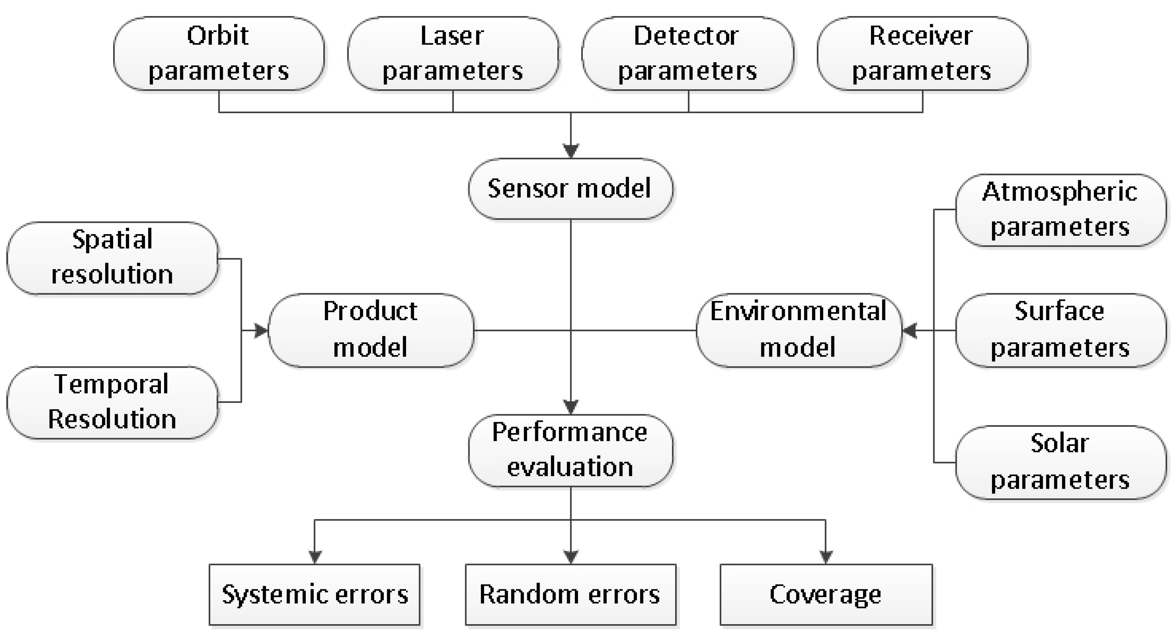
Figure 2.
Schematic diagram for the estimation of random errors.
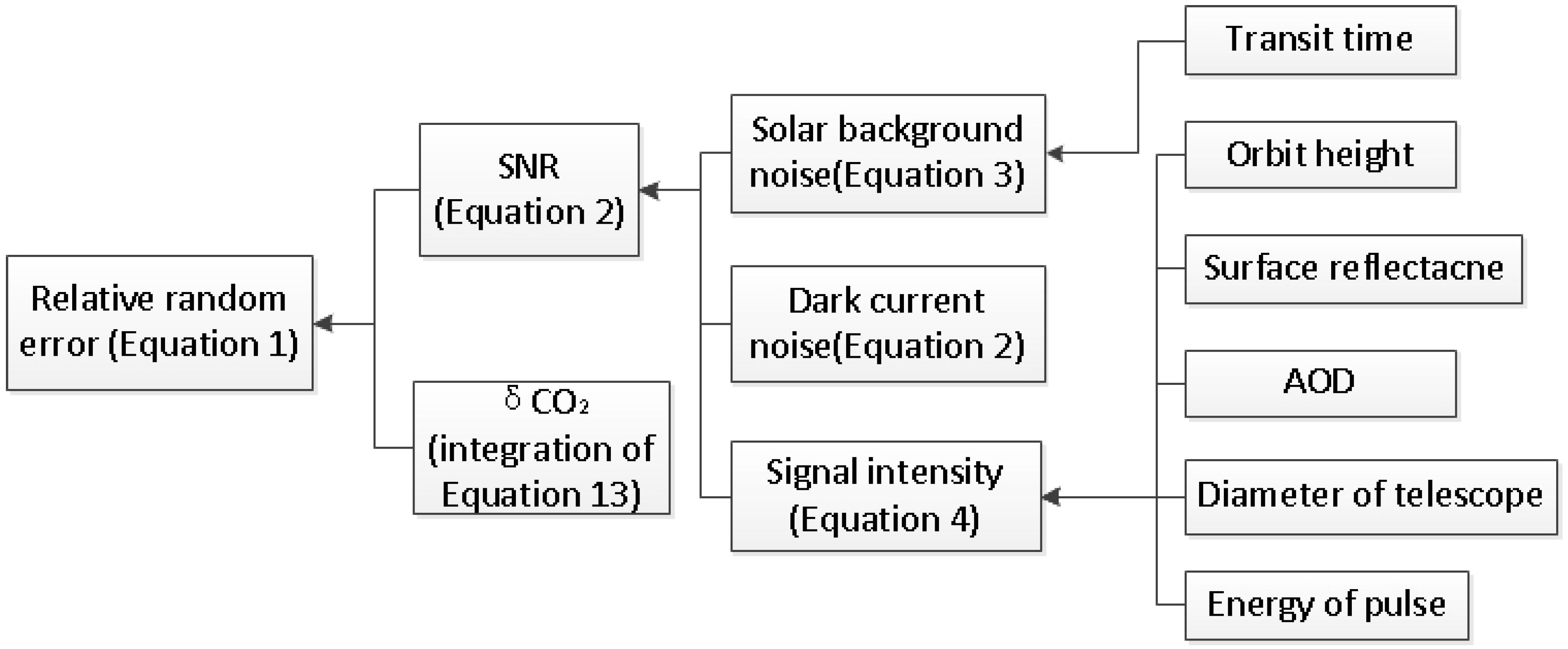
Figure 3.
The effect of orbit parameters on the relative random error. (a) The relationship between the orbit height and the relative random error. (b) The relationship between the solar radiance and the relative random error. (c) The combined effect of the two factors.
Figure 3.
The effect of orbit parameters on the relative random error. (a) The relationship between the orbit height and the relative random error. (b) The relationship between the solar radiance and the relative random error. (c) The combined effect of the two factors.

Figure 4.
Coverage of the CO2-IDPA for one month using different orbit altitudes. Red and yellow spots represent the nadirs collected using orbit altitudes of 450 and 705 km, respectively. The figure shows the base map (a), and the global distribution of 450 km (b) and 705 km (c) samples. (d,e) The regional distribution of nadir samples in Beijing and Tianjin.

Figure 5.
(a,b) Coverage of the CO2-IDPA for two months using different orbit altitudes. The symbols are as defined for Figure 4.
Figure 5.
(a,b) Coverage of the CO2-IDPA for two months using different orbit altitudes. The symbols are as defined for Figure 4.

Figure 6.
The effect of hardware parameters on the relative random error.

Figure 7.
The independent effects of reflectance and AOD on the performance of the CO2-IPDA. (a) shows Reflectance and (b) panel shows AOD.
Figure 7.
The independent effects of reflectance and AOD on the performance of the CO2-IPDA. (a) shows Reflectance and (b) panel shows AOD.

Figure 8.
The effect of environmental parameters on the relative random error.

Figure 9.
Yearly mean AOD values for China. The data source and the processing method are presented in Section 2.4. The data shown in Figure 9 are used as inputs for the evaluation model of relative random errors.
Figure 9.
Yearly mean AOD values for China. The data source and the processing method are presented in Section 2.4. The data shown in Figure 9 are used as inputs for the evaluation model of relative random errors.

Figure 10.
Yearly mean reflectance for China. The processing method for Figure 10 are presented in Section 2.4.
Figure 10.
Yearly mean reflectance for China. The processing method for Figure 10 are presented in Section 2.4.

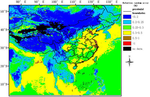
Figure 11.
Performance evaluation results. The relative random errors were calculated in terms of the schematic diagram shown in Figure 1. Parameters for the hardware model are from Table 3, shown in Section 2.5, and environmental parameters are shown in Figure 9 and Figure 10. The geographic extent of Figure 11 includes the whole territory of China and surrounding regions, including South Asia, the Korean peninsula, and Mongolia.

Figure 12.
Performance evaluation results. All parameters used to produce this figure are the same as those used in Figure 11 except the orbit height. The orbit height for Figure 11 is 705 km, while for this figure it is 450 km.
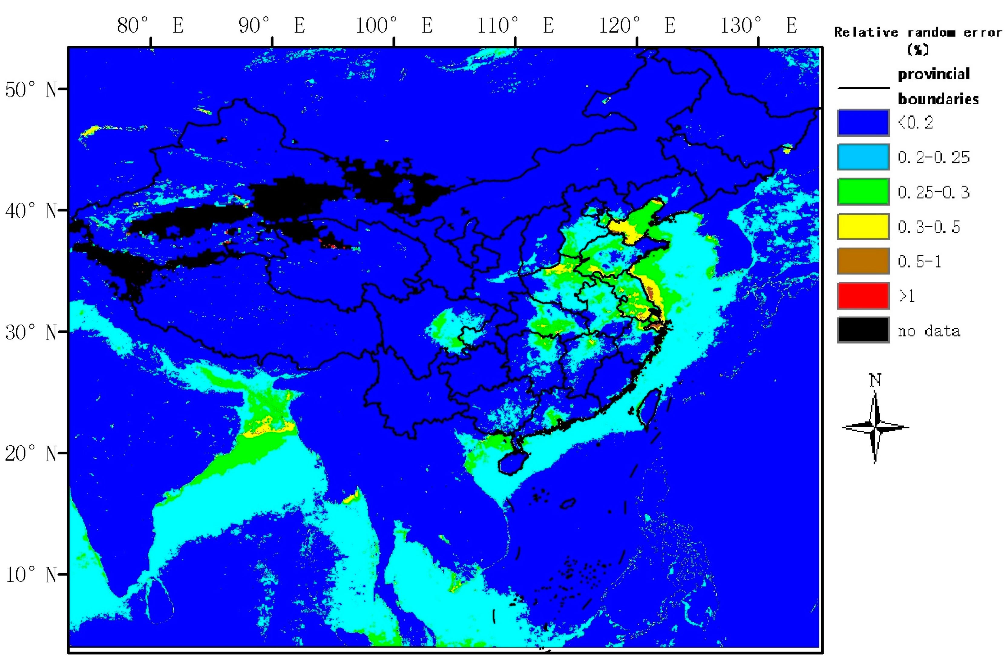
Figure 13.
Global atmospheric CO2 concentrations from 1 January to 11 November 2016, as recorded by National Aeronautics and Space Administration (NASA)’s Orbiting Carbon Observatory-2.
Figure 13.
Global atmospheric CO2 concentrations from 1 January to 11 November 2016, as recorded by National Aeronautics and Space Administration (NASA)’s Orbiting Carbon Observatory-2.

Figure 14.
Weighting functions (WF) for different wavenumbers: (a) shows the relationship between the WF and altitude. Different colors represent different wavenumbers as per the figure legend; In (b), the dotted curve denotes the spectrum for R18, and the colored straight lines represent the wavenumbers shown in the left-hand panel, using the same color key. The spectrum shown in the right-hand panel was calculated using T = 296 K and p = 101325 Pa, and the line has a Voigt shape.


Table 1.
Calculated systematic errors according to the configuration of the CO2-IPDA (integrated path differential absorption lidar).
Table 1.
Calculated systematic errors according to the configuration of the CO2-IPDA (integrated path differential absorption lidar).
| Category | Name | Uncertainty | Error a |
|---|---|---|---|
| atmospheric effect b | temperature | 0.5 K | 0.06 |
| pressure | 0.5 hPa | 0.11 | |
| humidity | 10% | 0.02 | |
| line parameter c | Line strength | 2% | 0.07 |
| Pressure shift | 1% | 0.08 | |
| Pressure broadening | 1% | 0.07 | |
| Temperature scaling exponent | 2% | 0.06 | |
| Laser d | Frequency drift | 0.6 MHz | 0.10 |
| spectral purity | 99.9% with a 0.45 nm filter | 0.24 | |
| fluctuation of ratio of on-line and off-line pulse energy e | 0.1% | - | |
| Satellite d | Doppler shift along track | 140 urad | 0.22 |
| Doppler shift across track | 1000 urad | 0.01 | |
| misalignment of footprint | 25 urad | 0.02 | |
| ranging accuracy | 2 m | 0.08 | |
| Total | 0.40 |
a the background value of XCO2 is set as 400 ppm and the unit of error is also ppm. b according to reference [30]. c according to reference [29]. d theoretical calculation by using equations presented in [29] and parameters herein. e the error derived from that factor is combined into the random error in this work.
Table 2.
Parameters for the orbit sampling equations.
| Name | Description/Value | Unit |
|---|---|---|
| δ | The latitude | degree |
| α | The longitude | degree |
| n | The angular velocity of satellite | rad/s |
| t | Any given time | s |
| t0 | The time at which the satellite passes the ascending node | s |
| Δα | The differential longitude between the ascending node and the current nadir | degree |
| ω | The angular velocity of earth/7.29 × 10−5 | rad/s |
| i | The orbit inclination/98.2 | degree |
| μ | The geocentric gravitational constant/3.986 × 1014 | m3/s2 |
| a | The semi-major axis of satellite orbit | km |
| Hsatellite | The altitude of satellite/705 or 450 in this work | km |
| Tsatellite | The orbit period | s |
Table 3.
Parameter configuration for China’s CO2-IPDA.
| Category | Parameter Name | Value | Unit |
|---|---|---|---|
| Laser Transmitter | Pulse length | 15 | ns |
| On-line wavelength | 6361.225 | cm−1 | |
| Off-line wavelength | 6360.981 | cm−1 | |
| Fluctuation of pulse energy | 1 | % | |
| Fluctuation of ratio of on-line and off-line pulse Energy | 0.1 | % | |
| Linewidth | 50 | MHz | |
| Stability of on-line wavelength | 0.6 | MHz | |
| Spectral purity | 99.9 | % | |
| Energy per pulse | 75 | mJ | |
| Repetition frequency(a pair of on-line and off-line) | 20 | Hz | |
| Divergence angle | 100 | urad | |
| Telescope | Time interval of contiguous pair | 0.2 | ms |
| Diameter | 1 | m | |
| Overall optical efficiency | 51.8 | % | |
| Optical filter bandwidth | 0.45 | nm | |
| Detector | Field of view | 0.2 | mrad |
| Electronic bandwidth | 3 | MHz | |
| Dark current(noise equivalent power) | 64 | fW/ | |
| Quantum efficiency | 73 | % | |
| Internal gain | 9 | mV/W | |
| Excess noise factor | 3.2 | - | |
| Other | Orbit altitude | 705 | km |
| Orbit type | 1 h/13 h sun-synchronous | - | |
| Viewing geometry | Nadir | - | |
| Reflectance over lands | 30 | % | |
| Reflectance over seas | 5 | % | |
| AOD | 0.3 | - | |
| RESOLUTION | 50 km (land)/100 km (ocean) | - |
Table 4.
Validation of XCO2 from OCO-2 with TCCON.
| Unit: PPM | Liang et al. [9] | Wunch et al. [34] | |||||||
|---|---|---|---|---|---|---|---|---|---|
| V7 | V7r | FP | |||||||
| Latitude | Bias a | RMS | Bias | RMS | Bias | RMS | Bias | RMS | N |
| 75 N–85 N | 2.06 | 2.54 | 2.37 | 3.20 | 0.58 | 2.26 | 0.10 | 1.99 | 3 |
| 60 N–70 N | 2.30 | 1.58 | 2.02 | 1.48 | 2.80 | 0.79 | 3.15 | 3.21 | 2 |
| 45 N–55 N | 0.73 | 2.49 | 0.05 | 2.31 | 0.41 | 1.52 | 0.78 | 1.74 | 180 |
| 30 N–40 N | 0.51 | 1.95 | 0.58 | 1.98 | 0.73 | 1.78 | 0.31 | 1.39 | 331 |
| 20 S–0 | 0.57 | 1.49 | 0.13 | 1.56 | 0.19 | 1.00 | 0.34 | 0.88 | 299 |
| 60 S–30 S | 0.45 | 2.43 | 0.02 | 2.28 | 0.01 | 1.51 | 0.28 | 1.37 | 799 |
| Global | 1.10 | 2.15 | 0.86 | 2.03 | 0.79 | 1.74 | 0.36 | 1.33 | / |
© 2017 by the authors. Licensee MDPI, Basel, Switzerland. This article is an open access article distributed under the terms and conditions of the Creative Commons Attribution (CC BY) license (http://creativecommons.org/licenses/by/4.0/).
Share and Cite
MDPI and ACS Style
Han, G.; Ma, X.; Liang, A.; Zhang, T.; Zhao, Y.; Zhang, M.; Gong, W. Performance Evaluation for China’s Planned CO2-IPDA. Remote Sens. 2017, 9, 768. https://doi.org/10.3390/rs9080768
AMA Style
Han G, Ma X, Liang A, Zhang T, Zhao Y, Zhang M, Gong W. Performance Evaluation for China’s Planned CO2-IPDA. Remote Sensing. 2017; 9(8):768. https://doi.org/10.3390/rs9080768
Chicago/Turabian StyleHan, Ge, Xin Ma, Ailin Liang, Tianhao Zhang, Yannan Zhao, Miao Zhang, and Wei Gong. 2017. "Performance Evaluation for China’s Planned CO2-IPDA" Remote Sensing 9, no. 8: 768. https://doi.org/10.3390/rs9080768
Note that from the first issue of 2016, this journal uses article numbers instead of page numbers. See further details here.