An Improved Spectrum Model for Sea Surface Radar Backscattering at L-Band


1
The Key Laboratory for Earth Observation of Hainan Province, Sanya 572029, China
2
State Key Laboratory of Remote Sensing Science, Institute of Remote Sensing and Digital Earth, Chinese Academy of Sciences, Beijing 100101, China
3
University of Chinese Academy of Sciences, Beijing 100049, China
*
Author to whom correspondence should be addressed.
Remote Sens. 2017, 9(8), 776; https://doi.org/10.3390/rs9080776
Submission received: 22 June 2017
/
Revised: 24 July 2017
/
Accepted: 27 July 2017
/
Published: 29 July 2017
(This article belongs to the Special Issue Ocean Radar)
Abstract
:L-band active microwave remote sensing is one of the most important technical methods of ocean environmental monitoring and dynamic parameter retrieval. Recently, a unique negative upwind-crosswind (NUC) asymmetry of L-band ocean backscatter over a low wind speed range was observed. To study the directional features of L-band ocean surface backscattering, a new directional spectrum model is proposed and built into the advanced integral equation method (AIEM). This spectrum combines Apel’s omnidirectional spectrum and an improved empirical angular spreading function (ASF). The coefficients in the ASF were determined by the fitting of radar observations so that it provides a better description of wave directionality, especially over wavenumber ranges from short-gravity waves to capillary waves. Based on the improved spectrum and the AIEM scattering model, L-band NUC asymmetry at low wind speeds and positive upwind-crosswind (PUC) asymmetry at higher wind speeds are simulated successfully. The model outputs are validated against Aquarius/SAC-D observations under different incidence angles, azimuth angles and wind speed conditions.
1. Introduction
L-band microwaves have a high sensitivity to marine physical parameters such as salinity and wind field [1]. Furthermore, due to their long wavelength, L-band microwaves have a good penetrability to adapt to complex surface conditions. L-band active microwave sensors are therefore widely-used in the measurement of ocean salinity and sea-surface wind fields, and have seen an increasing attention and development [2,3,4,5]. The first space-borne synthetic aperture radar (SAR) equipped on Seasat worked using L-band. Since then, several L-band active microwave sensors and missions have begun operation, which include the Japanese phased array type L-band synthetic Aperture Radar (PALSAR) [6], the Aquarius/SAC-D mission [7] and the Soil Moisture Active-Passive (SMAP) mission [8]. The Aquarius/SAC-D and SMAP missions, which were both undertaken by the U.S. National Aeronautics and Space Administration (NASA), have also used L-band microwave radiometers and combined active/passive L-band instruments for ocean research.
Currently, a number of geophysical model functions (GMFs) used to simulate ocean surface backscatter at L-band have been developed [5,6]. GMF is the model used to denote the quantitative transformation relationship between marine physical parameters, satellite observation geometry and normalized radar backscattering cross sections (NRCSs). These models have a high simulation accuracy in practical applications; however, GMFs are empirical models which have no definite physical meaning. Therefore, over the last several decades, some physically-based models were proposed and used to simulate the ocean surface scatter field; e.g., the Kirchhoff approximation (KA) model [9], the small perturbation method (SPM) [10], two-scale model (TSM) [11], small slope approximation (SSA) [12], integral equation method (IEM) [13,14] and the advanced integral equation method (AIEM) [15]. By solving the wave equation and making some approximations, these physically-based models were also called analytic approximate models (AAMs). AAMs can simulate the scatter field of a rough surface effectively in their specific scope of application. Among these AAMs, the IEM model and its improved AIEM model, with a strict physical meaning and high precision, have been used in various applications [16,17]. The IEM and AIEM model have also been utilized to simulate ocean surface microwave scattering. Chen et al. used IEM and the improved Fung-Lee spectrum to simulate the backscattering coefficients of the sea surface at the Ku-band and C-band; the results were in excellent agreement with the field measurements of the airborne scatterometer [18]. To better analyze the global navigation satellite system reflectometry (GNSS-R) signal, the bistatic scattering of the L-band in the sea is simulated by Fung et al. [19] by using IEM model. A backscattering model of the rough sea surface in a rainfall environment was proposed by Xu et al. [20] based on the IEM model and was verified by the C-band ENVISAT/ASAR data. All these successful applications of the IEM or AIEM have indicated the feasibility and advantages of this model in the simulation of ocean surfaces.
Recently, a unique upwind-crosswind (UC) asymmetry of the sea surface at L-band and low wind speed was observed by the space-borne scatterometers. Through the L-band geophysical model function developed for Aquarius/SAC-D, Yueh et al. [3] found that the NRCSs of the ocean surface at L-band versus wind direction show a negative upwind-crosswind (NUC) asymmetry of between approximately 3 and 8 m/s. However, the UC asymmetry appears positive at higher wind speeds or frequency bands. This feature was also confirmed by ALOS-PALSAR [6]. A conjecture that a new and unknown scattering mechanism which is different from Bragg and could account for this special feature was presented in [3]. In this study, we proposed a new explanation of this special UC asymmetry. A semi-empirical model which can simulate and interpret both the NUC and PUC asymmetry of L-band ocean backscatter is established, based on an improved directional spectrum and the AIEM model. Specifically, a new angular spreading function (ASF) is proposed to describe the anisotropy of sea waves. The proposed model is also validated against L-band scatterometer measurements.
2. Modeling
2.1. An Improved Directional Spectrum
Due to wind disturbance, a calm sea surface becomes rough, and the microwave signals emitted by the active microwave sensor can be back-scattered. Therefore, in order to simulate the ocean surface backscattering accurately, the establishment of a geometretical model of the rough sea surface generated by wind is the prime requirement; the accuracy of the sea surface geometry model determines the accuracy of the EM scattering model.
Currently, the sea surface morphology simulation methods are mainly based on the ocean wave spectrum. The elevation spectrum of ocean waves is defined as the Fourier transform of the autocorrelation of the sea surface height field [21]. It is one of the two-order statistical properties of stochastic processes and describes the distribution of each harmonic component of the sea surface with respect to the spatial frequency and orientation directly. The two-dimensional elevation spectrum is also called the directional spectrum or vector spectrum. The integration of the direction spectrum over the azimuth is defined as an omnidirectional spectrum, which is a one-dimensional spectrum and describes the distribution of the sea surface height energy at different wavenumbers. Generally, the omnidirectional spectrum often needs to be used first to obtain the two-dimensional directional spectrum. The relationship between the directional spectrum and omnidirectional spectrum is illustrated as
where k and φ are the wavenumber and wave direction relative to the wind, respectively. S(k) is the omnidirectional spectrum and S(k, φ) is the directional spectrum.
Over the past few decades, scholars have proposed a number of sea wave spectra. These spectra can simulate the sea surface morphology in the specific wind speed and wave number range and find successful applications for the EM scattering models [21,22,23,24,25,26]. Some early wave spectra are empirical formulations which are statistical descriptions of wind-generated surface waves. These spectra offer a better description of the longer gravity waves with measured data, despite the relatively low accuracy in the high wavenumber regime, by taking a simple experiential extension from gravity waves. However, for the EM scattering from the ocean surface, the primary contribution of the scattering is from the short-scale waves [27,28]. Therefore, an accurate description of short-gravity and capillary waves is also essential. To be consistent with the in situ observations of gravity-capillary waves, Apel [23] and Elfouhaily et al. [21] proposed a full wavenumber spectra based on the developed spectra. Kudryavtsev et al. derived a physical model of the short wind wave spectrum by analyzing the input and dissipation of sea wave energy based on the propagation theory of the spectral energy density [29]. Including scattering theory and radar data, the precise retrieval of short-wave spectral properties was implemented with active microwave observations [22,25,26,30]. Based on the technique of stereophotography and image brightness contrast processing, the directional short wind wave characteristics were measured and modeled [28,31,32]. Compared to former empirical spectra, these spectra can better describe the sea surface morphology in the short gravity-capillary wave wavenumber range.
To drive the AIEM model for sea surface backscattering, the geometrical parameters of the sea surface should be calculated by the omnidirectional spectrum. Only the improved Fung–Lee spectrum [18,22] and Elfouhaily spectrum [21] have been used to simulate the sea surface morphology and calculate the high-order spectra for this model. Nonetheless, the backscattering coefficient of the sea surface calculated by the IEM or AIEM model with the improved Fung–Lee spectrum was mainly at a high frequency; e.g., C-band and Ku-band. Meanwhile, although the IEM/Elfouhaily model was successfully used to simulate the L-band bistatic scattering of the sea surface [19], the accuracy of the Elfouhaily spectrum is relatively low in the low wind speed range. Among the numerous spectra mentioned previously, the Apel spectrum that was developed for the EM scattering model has a high accuracy in the full wavenumber and wide wind speed range. In particular, it performs well in our simulations of ocean surface microwave backscattering with the AIEM model. Therefore, in this paper, we choose the Apel omnidirectional spectrum as the basis for establishing our directional spectrum [23].
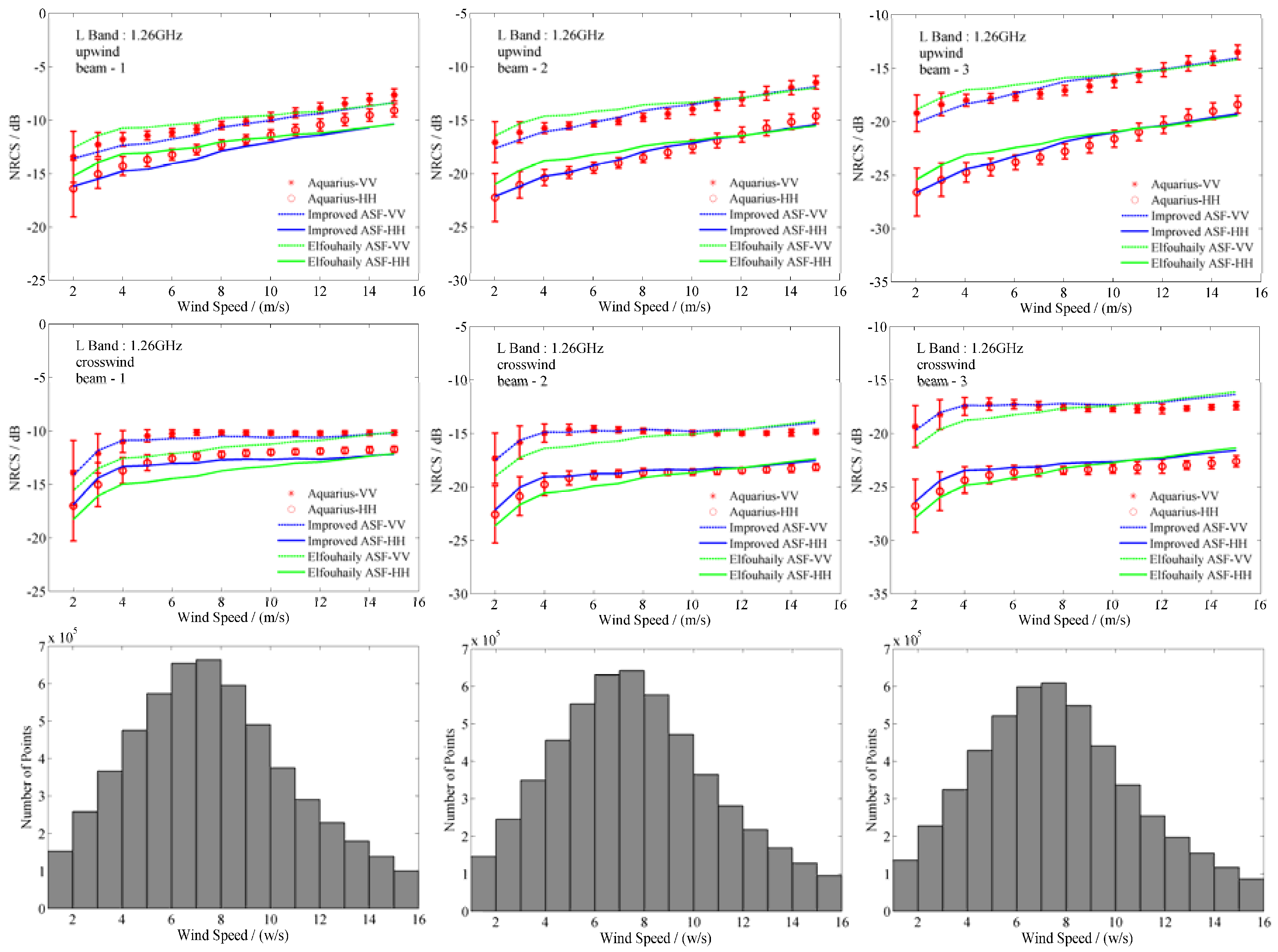
Figure 1 shows the Apel omnidirectional elevation spectrum for the full wavenumber range and for wind speeds from 3 to 21 m/s. The three vertical lines represent the microwave wavenumber k0 = 26.39 rad/m in 1.26 GHz, k0/10, k0*10, respectively. We believe that the sea waves in this range are the main waves which have interactions with the incident electromagnetic wave.
The two-dimensional directional spectrum is the Fourier transform of the bidimensional covariance of surface displacement, while the omnidirectional spectrum is one-dimensional [21]. To extend the one-dimensional omnidirectional spectrum to the two-dimensional directional spectrum, we multiply the omnidirectional spectrum by the angular spreading function (ASF) as
where Φ(k, φ) is the angular spreading function. The ASF describes the distribution of omnidirectional spectral energy in all directions under different wind speeds and different wave numbers so that it is the function of the wave number, wind speed and azimuth angle.
The first commonly used ASF was put forward by Longuet–Higgins [33] which is a cosine-shape parametric function which was improved by Mitsuyasu et al. [34]. Over the following decades, continuous improvements were made by Donelan et al. [25], Fung and Lee [22], Nickolaev et al. [35], Apel et al. [23] and Elfouhaily et al. [21], etc. However, these ASFs have a different noncentrosymmetry, and different spreading functions have diversities of mathematical properties. This introduces a number of difficulties for the use of a directional spectrum in sea surface scattering modeling. To overcome these difficulties, Elfouhaily et al. [21] put forward an angular spreading function based on the first two order harmonics of Fourier series expansion. This solution offers useful mathematical properties; e.g., the normalization of azimuth integral and central symmetry. This improved ASF function can be written as
In Equation (3), Δ(k) is upwind-crosswind ratio that can be calculated from an already developed ASF regardless of whether it is centrosymmetric. Δ ratio describes the anisotropy of the spreading functions and depends on wavenumber k.
With Equation (4), different spreading functions that are already developed can be unified in Δ ratios which are similar in form. Furthermore, these functions can be turned into the form as Equation (3). For the sake of simplicity, we will not give the specific developed ASFs and their Δ ratios here, but the numerical curves of Δ ratios corresponding to the ASFs are shown in Figure 2a.
Radar observation results indicate that the gravity waves have an obvious directionality, while the short-gravity waves lose their directionality gradually with the decrease of the wavelength. However, when the wave wavenumbers decrease into the gravity-capillary range, the waves become more directional again [21,36]. Although it is generally believed that small-scale waves are almost isotropic, the directionality of the gravity-capillary waves observed by the radar can be explained by hydrodynamic modulation due to large-scale waves. Therefore, to better describe the directionality of ocean waves based on the developed ASFs, Elfouhaily et al. [21] suggested a Δ ratio formula in the hyperbolic tangent form for a full wavenumber range spreading function as
where c is the wave phase speed and cp is the phase speed of the dominant long wave. a0 and ap are constants that equal ln(2)/4 and 4, respectively. am is expressed as
where u* is the friction velocity at the sea surface and cm is the minimum phase speed at the wavenumber of the gravity-capillary peak. In Equation (5), the first two items of the hyperbolic tangent function describe the anisotropy of the gravity waves and short-gravity waves of the ocean surface while the third item determines the anisotropy of gravity-capillary waves.
The Elfouhaily spreading function can appropriately describe the directionality of long gravity waves and short capillary waves. Thus, it was used in some microwave scattering models to simulate radar azimuth anisotropy [19]. However, for a special wavelength range, i.e., from short-gravity waves to capillary waves, the sea surface backscattering characteristics still cannot be explained and simulated by the existing ocean wave spectra and analytic approximate models.
Recent observations and studies have discovered that in the 3–9 m/s range of wind speed, the L-band backscatter versus the relative wind direction has a NUC asymmetry. This means that the normalized radar cross sections (NRCSs) at the crosswinds are larger than those upwind or downwind, while the upwind-crosswind asymmetry at high-frequency bands or at above 10 m/s wind speed is positive [3]. This phenomenon has been verified by several operated space-borne L-band scatterometers equipped on ALOS, Aquarius and SMAP [2,6]. However, there are thus far no theories or analytic models that can simulate this phenomenon [2,3]. Some scholars have suspected that the phenomenon is caused by an unknown scattering mechanism which is different from Bragg and dominates at low winds [3]. In this paper, we believe the cause of this unusual phenomenon is the difference of wave directionality in the specific wavenumber range, while the scattering mechanism is still Bragg.
In fact, at moderate and low wind speeds, the directionality of waves generated by the wind changes in the short gravity-capillary wave wavenumber range. Consequently, the directionality of some small-scale waves is contrary to that in the large-scale wave wavenumber range. This means that the numbers of small-scale waves that propagate perpendicular to the wind direction are larger than those along the wind direction. This phenomenon has been confirmed by several observations. In the experiment of Banner et al. [37], their two-dimensional spectrum for short gravity waves shows a greater power spectral density at crosswind than alongwind. Hara et al. [38] found that gravity waves (k = 49 rad/m) may exist and propagate against the wind from their observed spectra, and this can lead to a similar conclusion as Banner et al. [37]. Further, the fitting procedure of the Δ ratio showed negative values in the short gravity wavenumber range, which means that the energy of the spectrum in the crosswind direction can exceed the energy in the alongwind direction [28]. There are no convincing physical explanations for this phenomenon [37,38]; however, some scholars have illustrated a number of kinetic characteristics of small-scale waves that can be instructive. Elfouhaily et al. [21] demonstrated that a few of the shorter waves ridden on longer waves may travel perpendicular to the wind direction due to the interaction between wave. For the same reason, Donelan et al. [39] and Hara et al. [38] believe that some short waves even propagate against the wind direction. Mitsuyasu et al. [34] measured the wave characteristics by buoys under several steady sea conditions. According to the measurements, they found that in a steady wind direction, the wave directionality changes with the decreasing wavelength.
Since most of the existing ASFs do not describe the peculiar directionality of the short gravity waves, we mathematically construct an improved angular spreading function based on Elfouhaily’s Δ ratio formula. The Δ ratio formula of our spreading function is shown as
where, different from Equation (5), the constant a0 equals −ln(2)/4. The second item of the hyperbolic tangent function describes the directionality of short-gravity waves which is contrasted with long-gravity waves with the constant ad = ln(2)/2. Sd also has a hyperbolic tangent shape and a wind speed dependency that is expressed as
where u* is the friction velocity. kx is a function of the wavenumber as
with the minimum phase speed, cm = 0.23 m/s.
In Equation (7), the last two items of the hyperbolic tangent function are basically the same as those of Elfouhaily’s Δ ratio formula. However, the constant am in the last item equals 0.26 by multiplying a factor of two by Elfouhaily’s am = 0.13.
The core of our Δ ratio formula shown as Equation (7) is the second item in the square brackets, which produces the negative part in the range of short gravity waves. This item is constructed mathematically to simulate the directionality of the waves coupled with L-band microwaves. The hyperbolic tangent function is chosen to restrain the energy of the function body. The V-shaped part of our Δ ratio is produced by the “hook function”, which has a general form as . When a > 0 and b > 0, the “hook function” has an extreme point at () in the first quadrant. According to the relationship between scattering directionality and wind velocity, the V-shaped function is constructed with a dependency on the friction velocity and the wavenumber of the spectral peak. The wavenumber of the spectral peak kp is expressed as wave phase speed with the relation written as
Thus, the V-shaped “hook function” is shown as the first two items of the hyperbolic tangent function in Equation (8). The exponents defined in Equation (9) stretch the wavenumber k on the axis. Based on the properties of the “hook function”, the last two items of the hyperbolic tangent function in Equation (8) are constructed to tailor the V-shaped part of Δ ratio to the directionality of L-band microwave backscattering. Further, the coefficients in Equations (8) and (9) are determined by fitting simulations of scattering model and the L-band radar observations (as shown in Section 3).
Figure 2b shows the numerical curve of our Δ ratio formula in the full band range. The corresponding wind speed is from 3 to 15 m/s with a 2 m/s interval. The middle vertical line represents the microwave wavenumber k0 = 26.39 rad/m in 1.26 GHz while the left and right vertical lines represent the waves wavenumber, 2k0sin(20°) and 2k0sin(60°), respectively. They are the wavenumbers of sea surface waves which resonate with the L-band microwaves (1.26 GHz) at 20° and 60° incidence angles, according to the Bragg scattering mechanism. As seen from the curves in Figure 2b, the value of the Δ ratio has both positive and negative aspects which represent opposite wave directionalities for different wavenumbers. In fact, by combining Equations (3) and (4), we may conclude that the absolute value of the Δ ratio decides the wave anisotropy, while the positive and negative of Δ ratio dominates the wave directionality. Therefore, as opposed to most developed spreading functions, the V-shaped part in our Δ ratio curve simulates the special directionality of the short-gravity waves that have been shown in the L-band scattering signals. The V-shaped part in our Δ ratio curve shifts towards the longer wavelength with the increase of the wind speed. During the wavenumber range (between the left and right vertical lines) with which we are concerned, the Δ ratio has negative values at low wind speeds and positive ones at higher speeds. This corresponds to the fact that the NUC asymmetry appears at low speeds while the PUC asymmetry appears at higher speeds. However, the Δ ratio values are almost positive at higher wavenumbers, which may be coupled with higher frequency microwaves; e.g., the C band and Ku band. This explains why the upwind–crosswind asymmetry is positive at high-frequency bands. In addition, the absolute value of the Δ ratio during the wavenumber range between the two vertical lines increases in the 3–5 m/s wind speed range, decreases in the 5–8 m/s wind speed range, and goes up above the 9 m/s wind speed again. This pattern agrees exactly with the change of peak-to-peak radar backscattering variations.
However, it should be noted that the application of our ASF will only focus on the L-band and higher frequencies. With limited observations, our ASF puts more energy in the crosswind direction for gravity waves, which does not conform to the actual situation. Therefore, in the future extension of this study, more in situ measurements or radar observations at lower wavenumbers are needed to extend application range of this ASF [37,38].
Figure 3a–f illustrates, in polar coordinates, the numerical curve of Elfouhaily ASF and our function at 5 m/s wind speed and different wavenumbers, respectively. We can see that the curve shapes of the two ASFs are almost the same in the long-gravity wavenumber range and are slightly different in the capillary wavenumber range. However, the difference between the two ASF curves in the short-gravity wavenumber range is quite large. Our ASF seems to simulate the special directionality during this band range better and is more suitable for an analytical model.
Based on the modeling of sea surface morphology, the geometrical parameters of the ocean surface can be calculated and put into an EM scattering model as described in the following section.
2.2. Scattering Model
The advanced integral equation method (AIEM) is a full analytical model used to simulate the scattering field of a random rough surface. It was developed by Chen et.al. [15] based on the integral equation method (IEM) [13]. The backscattering coefficients of vertical and horizontal polarization calculated by AIEM model are expressed as
where ke and θ are the wavenumber and microwave incidence angles of exploring microwaves. δ is the sea surface morphology parameter that represent the root mean square height. The subscript p can be V or H which denotes vertical or horizontal polarization. is the high-order surface spectrum with , which is the wavenumber of the surface harmonic generatinf Bragg resonance with the incident microwave. For the sake of simplicity, we will not present the specific forms of all coefficients here; they can be found in [40] with additional details.
In this model, δ and describe the geometry of rough surfaces and are important input parameters. Therefore, the key to applying the AIEM model to the simulation of sea surface backscattering is the method of calculating the morphology parameters of the sea surface.
Because the ocean wave spectrum is defined and used to simulate the sea surface morphology, the geometric parameters of a rough ocean surface can be calculated from it. The mean deviation of surface elevations δ2 is given as
However, the mean deviation calculated by Equation (12) cannot be directly used in the AIEM model as shown in Equation (11) as it is the result of the full amount of wavenumber waves. In fact, the exploring microwave does not couple with all wavelength waves but a specific wavenumber range of waves which have comparable roughness scales to the microwave wavelength [19,41]. It means that only a range of roughness scales is effective in generating scattering. Hence, the geometric parameters inserted into the AIEM model should represent the characteristics of the waves coupled with microwaves. According to the Bragg scattering theory, this wavenumber range is a function of exploring the wavelength and incident angle. In practical computations, this range also depends on the selection of scattering model and wave spectrum. The range for the IEM/Fung–Lee model was suggested by Xu et al. [20] and Marrazzo et al. [42] as (k0*0.4, k0*10). Accordingly, by comparing with the in situ measured sea surface geometric data and the satellite observations, we generally believe that the wavenumber range of waves coupled with microwaves is between k0/10 and k0*10, where the microwave wavenumber k0 = 26.39 rad/m in 1.26 GHz (also shown in Figure 1). Notably, this wavenumber range is only chosen to calculate the geometry parameter (δ) for the AIEM model and has a different meaning from the spectrum cutoff used in TSM. Also, it is independent of the wind speed and exploring frequency. Additionally, the waves in this range are also believed to determine sea surface emissivity [4].
The high-order surface spectrum is defined as the two-dimensional Fourier transform of the nth power of the surface autocorrelation function. Therefore, is expressed as
where ρ(r, ϕ) is the normalized autocorrelation function of the ocean surface in the polar coordinate with the lag distance r and azimuth angle ϕ, which are related to wave direction. ρ(r, ϕ) describes the geometric features of rough surfaces in the space dimension.
For the sea surface, the wave spectrum is the Fourier transform of the autocorrelation of the sea surface displacements. We can obtain the sea surface autocorrelation function by the inverse Fourier transform of the wave spectrum. The transform is
The calculations of the surface autocorrelation and the high-order spectrum are operated in the full wavenumber range.
With sea surface morphology parameters calculated by our improved directional spectrum, the L-band ocean backscattering can be simulated by AIEM model.
3. Validation and Discussion
3.1. Data Description
Aquarius/SAC-D is a satellite co-operated by NASA and the Argentina Space Agency (CONAE) which is committed to obtaining global sea surface salinity data. It was launched on 10 June 2011 and came into full operation on 25 August of that year. Unfortunately, this satellite ended its mission prematurely due to the failure of the power support system and attitude control system. During its period of operation, a large number of the ocean observation data was obtained, and its data at all levels were distributed by PO.DAAC at the Jet Propulsion Laboratory (JPL).
The Aquarius instrument has three antennas whose incident angles are 28.7°, 37.8° and 45.6°, respectively [3,43]. These antennas are shared by the L-band microwave radiometer operating at 1.413 GHz and the scatterometer operating at 1.26 GHz. To validate the simulation of the L-band sea surface backscattering with our model, the Aquarius V4.0 L2 data from all of 2014 were collected. These L2 data include sensor-measured data, retrieval products and the related ancillary data of each track. The measurements of the scatterometer provided by the data set were used to validate the model calculation results. In addition, several sea surface dynamic physical parameters included in the data set would also be the input of our model; i.e., the sea surface temperature (SST) from the NOAA optimum interpolation sea surface temperature (OISST) product, the sea surface salinity (SSS) from the hybrid coordinate ocean model (HYCOM) and the sea surface wind field from the NCEP global forecast system (GFS).
3.2. Results and Discussion
The sea surface NRCSs at L-band were calculated with the improved wave spectrum and AIEM model. The results were compared to the Aquarius observations. Specifically, in the calculation process, the dielectric constants needed by the AIEM model were obtained from the K-S model [44]. The model inputs were SST and SSS, which were provided by the ancillary data in the Aquarius L2 data set.
In Figure 4, the VV and HH sea surface NRCSs at L-band versus the relative wind direction were compared to Aquarius observations for different wind speeds. Meanwhile, the mean biases between model simulations and satellite observations were calculated at multiple wind velocities, polarizations and incidence angles. Specifically, each row represents a different wind speed, i.e., 3, 5, 8, 10, 12, 15 m/s, while the columns correspond to three antenna beams. In general, our model results have a good concordance with the satellite observations. Almost all mean biases are less than 1 dB, and most maximal biases are restrained in 1 dB. For an analytical approximate model, these indicate a good accuracy of our model at L-band [17,20,23,24]. In the range of 3–8 m/s wind speed, the NUC asymmetry of the L-band sea surface backscatter, which may also be called “M-shape” feature, was simulated well. As is shown in Figure 2b, the sea waves show the most obvious NUC asymmetry in the concerned wavenumber range, due to the Δ ratios decreasing with wind speed increasing and the minimum of Δ ratios at 5 m/s wind speed. The peak-to-peak variations of NRCSs are up to 1 dB and 0.7 dB for VV polarization and HH polarization at beam 1. The peak-to-peak amplitude decreases in the 5–8 m/s range. For wind speeds above 8 m/s, the upwind–crosswind asymmetry turns positive, which we call the “W-shape” feature in model simulations and observations. The peak-to-peak amplitudes increase as the wind speed increases because the Δ ratios are positive and increase as the wind speed increases. It should also be noted that, in the 3–8 m/s range, the NRCSs have smaller peak-to-peak amplitudes at the larger incidence, while the opposite is true above the 8 m/s wind speed. This phenomenon can be explained by the absolutes of Δ ratios in the concerned range at different wind speeds. The absolutes of Δ ratios decrease in the 3–8 m/s range while increasing in the 9–15 m/s range, with wavenumber increasing; this corresponds to the increase of the incident angle. At a 15 m/s wind speed, the model simulations are larger than the observations at a crosswind while they are smaller than observations at upwind, which suggests that the peak-to-peak amplitude of the model result is smaller than that of the observation. In the analysis of the next section, this limitation is revealed and interpreted. It denotes that the Δ ratio of our angular spreading function should be larger at high wind speeds. In addition, the transition between the “M-shape” feature and “W-shape” feature can be noticed at an 8 m/s wind speed, which indicates the transition of the Δ ratio between the negative portion and positive portion. Our model simulations show a slightly stronger directionality than Aquarius observations at beam 2 and 3. Similarly, at 3 m/s, model results also show stronger directionality. These phenomena will be numerically analyzed in next section.
During the 9–15 m/s wind speed range, however, our model simulations at beam 1 are slightly smaller than the observations, especially for HH polarization. Additionally, at beam 2 and beam 3, the NRCSs simulated by the model are larger than the observations in the downwind direction due to ignoring the skewness effect of sea waves [18,45,46,47].
To further demonstrate the advantages of our improved spectrum in describing the wave directionality in the range of interest, we compared the azimuthal features of model simulations with Elfouhaily’s ASF and our ASF at two specific wind speeds in Figure 5. In reality, the difference of these two ASFs lies in the Δ ratio formulae, which are given in Equations (5) and (7). The wind speed at 5 and 12 m/s were chosen to represent low and high wind speeds, respectively. In general, the AIEM model with our ASF can simulate both the NUC asymmetry at low wind speeds and the PUC asymmetry at higher wind speeds, while it only shows PUC asymmetry at all wind speeds with Elfouhaily’s ASF. At 5 m/s, it can obviously be seen that the model simulations with two different ASFs show almost opposite UC asymmetries. Clearly, by comparing with the satellite observations, model NRCSs calculated with our ASF simulate the NUC asymmetry of L-band ocean surface backscattering successfully, and the simulations with Elfouhaily’s ASF lead to erroneous PUC at low wind speed. However, at 12 m/s, the model simulations with two ASFs are similar and describe the real azimuthal features of sea surface backscattering at all three incidences. Therefore, we may draw the conclusion that our improved ASF shows superiority for wave directionality description at lower wind speeds. This fact will be further illustrated in the following analysis.
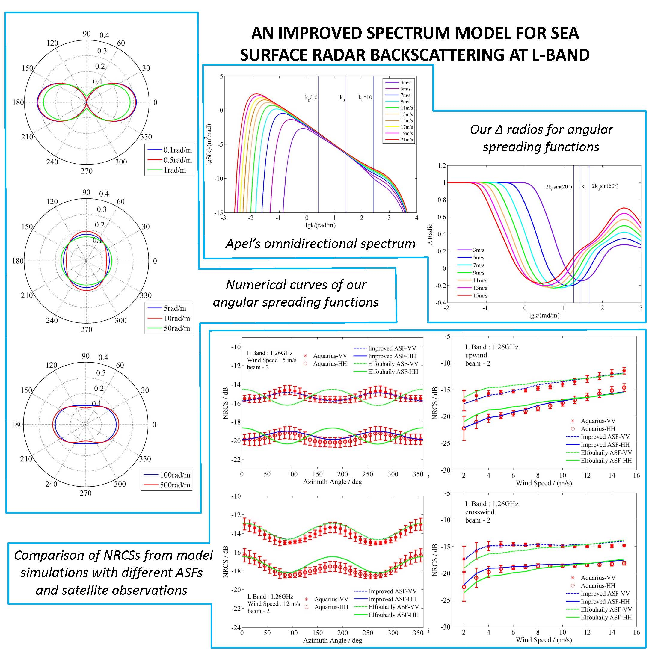
In Figure 6, the model NRCSs calculated with two different ASFs versus the wind speed were also compared to Aquarius observations in the upwind and crosswind direction. As the figures show, at all three beams, the model results using our improved ASF agree with the observations well, which indicate that our ASF has a better description of the directionality of the continuous gravity-capillary waves coupled with L-band microwaves. In addition, the model simulations with two ASFs show obvious gaps at low wind speeds, while they are close at high wind speeds. This also expresses the advantages of our ASF in the low wind speed range. It should be also noted that the L-band sea surface NRCSs keep increasing as the wind speeds increase in the upwind direction. However, the NRCSs in the crosswind direction increase only during the low wind speed range and remain almost steady at higher wind speeds. This suggests that the energy remains conserved for waves during the wavenumber range which are coupled with the incident microwave. A comparison with Aquarius observations shows that model simulations with our spectrum describe this feature well.
3.3. Numerical Analysis of Scattering Directionality
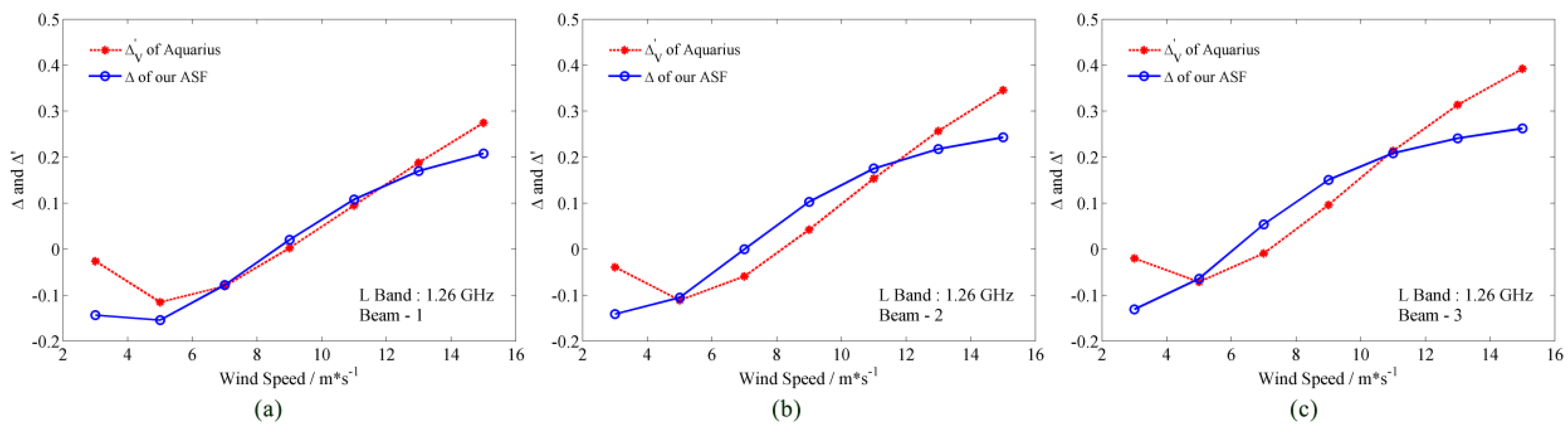
According to Bragg scattering theory, the directionality of ocean surface backscattering is dominated by the directionality of waves around Bragg wavenumbers; specifically, the Δ radio in ASF. Therefore, to quantitatively evaluate the directionality of ocean surface microwave backscattering calculated by our model, here an index similar to the Δ ratio is proposed as
where , and represent the backscattering coefficients at upwind, downwind and crosswind, respectively. is defined in liner unit.
In Figure 7, our Δ radio and the Δ′ calculated by Aquarius observations are compared as a function of wind speed at three beams. As the figures show, the generally good agreements of Δ and Δ′ demonstrate that our semi-empirical model with a new ASF can simulate the NUC and PUC of ocean surface backscattering well. However, it should be noted that at 3 m/s and 15 m/s, Δ are less than Δ′, but the absolutes of Δ are larger and less than Δ′, respectively. This numerical feature explains the stronger and weaker directionality of our model simulations at 3 m/s and 15 m/s. Similarly, at beam 2 and 3, the larger absolute value of Δ at 8 m/s indicates the stronger directionality of our model results.
4. Conclusions
In this paper, a new interpretation of the unique NUC asymmetry of L-band sea surface backscatter in a low wind speed range is presented. Furthermore, an improved ocean wave spectrum is proposed by combining Apel’s omnidirectional spectrum and a new angular spreading function. This new spectrum can better describe the directionality of waves, especially for waves coupled with L-band microwaves. Subsequently, a semi-empirical model which merged this improved spectrum into the AIEM scattering model has been established to simulate the anisotropy and directionality of the sea surface backscatter. Specifically, the wavenumber scope of waves that interact with the incident microwave is determined to calculate the surface morphology parameters, and the high-order spectra for the model are obtained by the Fourier transform of the surface autocorrelation function. The model simulates the L-band NUC asymmetry at low wind speeds and the PUC asymmetry at higher wind speeds successfully; the transition between these two asymmetries is also revealed. However, at several specific wind speeds, our model simulations show a slightly stronger or weaker directionality than Aquarius observations. The comparisons between our model simulations and the Aquarius satellite observations show a good consistency. Besides this, the comparisons of model simulations with our and Elfhouhaily’s ASF indicate the improvement and superiority of our directional spectrum in describing the wave directionality in the concerned wavenumber range. In general, our model has a good performance in simulating L-band ocean surface backscattering and interpreting its NUC and PUC asymmetry.
In the future, we are planning to take the skewness of waves into consideration to simulate the directional difference between the upwind direction and downwind direction. Besides this, more in situ measurements at lower wavenumbers will be included to extend the application range of our directional spectrum. These future works would broaden the applicability of this spectrum.
Acknowledgments
This study is supported by the National Natural Science Foundation of China (Grant No. 41531175), and the Key Research and Development Program of Hainan Province (Grant No. ZDYF2017167). The authors would like to thank F. Xu from Fudan University for his valuable discussion and the anonymous reviewers for their constructive comments. The Aquarius L2 data were provided by NASA PO.DAAC at the Jet Propulsion Laboratory (http://podaac.jpl.nasa.gov/SeaSurfaceSalinity/Aquarius).
Author Contributions
Yanlei Du, Xiaofeng Yang, Kun-Shan Chen and Ziwei Li conceived and designed the experiments; Yanlei Du performed the experiments; Yanlei Du, Wentao Ma analyzed the data; Yanlei Du and Xiaofeng Yang wrote the paper.
Conflicts of Interest
The authors declare no conflict of interest.
References
- Yueh, S.H.; Chaubell, J. Sea surface salinity and wind retrieval using combined passive and active L-band microwave observations. IEEE Trans. Geosci. Remote Sens. 2012, 50, 1022–1032. [Google Scholar] [CrossRef]
- Meissner, T.; Wentz, F.J.; Ricciardulli, L. The emission and scattering of L-band microwave radiation from rough ocean surfaces and wind speed measurements from the Aquarius sensor. J. Geophys. Res.-Oceans 2014, 119, 6499–6522. [Google Scholar] [CrossRef]
- Yueh, S.H.; Tang, W.Q.; Fore, A.G.; Neumann, G.; Hayashi, A.; Freedman, A.; Chaubell, J.; Lagerloef, G.S.E. L-band passive and active microwave geophysical model functions of ocean surface winds and applications to Aquarius retrieval. IEEE Trans. Geosci. Remote Sens. 2013, 51, 4619–4632. [Google Scholar] [CrossRef]
- Ma, W.T.; Yang, X.F.; Yu, Y.; Liu, G.H.; Li, Z.W.; Jing, C. Impact of rain-induced sea surface roughness variations on salinity retrieval from the Aquarius/SAC-D satellite. Acta Oceanol. Sin. 2015, 34, 89–96. [Google Scholar] [CrossRef]
- Yueh, S.H.; Dinardo, S.J.; Fore, A.G.; Li, F.K. Passive and active L-band microwave observations and modeling of ocean surface winds. IEEE Trans. Geosci. Remote Sens. 2010, 48, 3087–3100. [Google Scholar] [CrossRef]
- Isoguchi, O.; Shimada, M. An L-band ocean geophysical model function derived from PALSAR. IEEE Trans. Geosci. Remote Sens. 2009, 47, 1925–1936. [Google Scholar] [CrossRef]
- Lagerloef, G.; Colomb, F.R.; Le Vine, D.; Wentz, F.; Yueh, S.; Ruf, C.; Lilly, J.; Gunn, J.; Chao, Y.; de Charon, A.; et al. The Aquarius/SAC-D mission: Designed to meet the salinity remote-sensing challenge. Oceanography 2008, 21, 68–81. [Google Scholar] [CrossRef]
- Spencer, M.; Wheeler, K.; White, C.; West, R.; Piepmeier, J.; Hudson, D.; Medeiros, J. The soil moisture active passive (SMAP) mission L-band radar/radiometer instrument. In Proceedings of the 2010 IEEE International Geoscience and Remote Sensing Symposium, Honolulu, HI, USA, 25–30 July 2010; pp. 3240–3243. [Google Scholar]
- Bruce, N.C.; Dainty, J.C. Multiple-scattering from random rough surfaces using the kirchhoff approximation. J. Mod. Opt. 1991, 38, 579–590. [Google Scholar] [CrossRef]
- Sotocrespo, J.M.; Nietovesperinas, M.; Friberg, A.T. Scattering from slightly rough random surfaces—A detailed study on the validity of the small perturbation method. J. Opt. Soc. Am. A 1990, 7, 1185–1201. [Google Scholar] [CrossRef]
- Khenchaf, A.; Daout, F.; Saillard, J. The two-scale model for random rough surface scattering. In Proceedings of the Oceans ‘96 MTS/IEEE Conference Proceedings, Prospects for the 21st Century, Fort Lauderdale, FL, USA, 23–26 September 1996; Volumes 1–3, pp. 887–891. [Google Scholar]
- Voronovich, A. Small-slope approximation for electromagnetic-wave scattering at a rough interface of dielectric half-spaces. Wave Random Media 1994, 4, 337–367. [Google Scholar] [CrossRef]
- Fung, A.K.; Li, Z.Q.; Chen, K.S. Backscattering from a randomly rough dielectric surface. IEEE Trans. Geosci. Remote Sens. 1992, 30, 356–369. [Google Scholar] [CrossRef]
- Fung, A.K.; Tjuatja, S. Backscattering and emission signatures of randomly rough surfaces based on IEM. In Proceedings of the 1993 International Geoscience Remote Sensing Symposium (IGARSS ’93), Better Understanding of Earth Environment, Tokyo, Japan, 18–21 August 1993; pp. 1006–1008. [Google Scholar]
- Chen, K.S.; Wu, T.D.; Tsang, L.; Li, Q.; Shi, J.C.; Fung, A.K. Emission of rough surfaces calculated by the integral equation method with comparison to three-dimensional moment method simulations. IEEE Trans. Geosci. Remote Sens. 2003, 41, 90–101. [Google Scholar] [CrossRef]
- Chen, K.S.; Wu, T.D.; Shi, J.C. A model-based inversion of rough soil surface parameters from radar measurements. J. Electromagn. Wave 2001, 15, 173–200. [Google Scholar] [CrossRef]
- Chen, K.S.; Fung, A.K.; Amar, F. An empirical bispectrum model for sea-surface scattering. IEEE Trans. Geosci. Remote Sens. 1993, 31, 830–835. [Google Scholar] [CrossRef]
- Chen, K.S.; Fung, A.K.; Weissman, D.E. A backscattering model for ocean surface. IEEE Trans. Geosci. Remote Sens. 1992, 30, 811–817. [Google Scholar] [CrossRef]
- Fung, A.K.; Zuffada, C.; Hsieh, C.Y. Incoherent bistatic scattering from the sea surface at L-band. IEEE Trans. Geosci. Remote Sens. 2001, 39, 1006–1012. [Google Scholar] [CrossRef]
- Xu, F.; Li, X.F.; Wang, P.; Yang, J.S.; Pichel, W.G.; Jin, Y.Q. A backscattering model of rainfall over rough sea surface for synthetic aperture radar. IEEE Trans. Geosci. Remote Sens. 2015, 53, 3042–3054. [Google Scholar] [CrossRef]
- Elfouhaily, T.; Chapron, B.; Katsaros, K.; Vandemark, D. A unified directional spectrum for long and short wind-driven waves. J. Geophys. Res.-Oceans 1997, 102, 15781–15796. [Google Scholar] [CrossRef]
- Fung, A.K.; Lee, K.K. A semi-empirical sea-spectrum model for scattering coefficient estimation. IEEE J. Ocean. Eng. 1982, 7, 166–176. [Google Scholar] [CrossRef]
- Apel, J.R. An improved model of the ocean surface-wave vector spectrum and its effects on radar backscatter. J. Geophys. Res.-Oceans 1994, 99, 16269–16291. [Google Scholar] [CrossRef]
- Durden, S.L.; Vesecky, J.F. A physical radar cross-section model for a wind-driven sea with swell. IEEE J. Ocean. Eng. 1985, 10, 445–451. [Google Scholar] [CrossRef]
- Donelan, M.A.; Pierson, W.J. Radar scattering and equilibrium ranges in wind-generated waves with application to scatterometry. J. Geophys. Res.-Oceans 1987, 92, 4971–5029. [Google Scholar] [CrossRef]
- Kudryavtsev, V.; Hauser, D.; Caudal, G.; Chapron, B. A semiempirical model of the normalized radar cross section of the sea surface, 2. Radar modulation transfer function. J. Geophys. Res.-Oceans 2003, 108. [Google Scholar] [CrossRef]
- Hwang, P.A. A note on the ocean surface roughness spectrum. J. Atmos. Ocean. Technol. 2011, 28, 436–443. [Google Scholar] [CrossRef]
- Yurovskaya, M.V.; Dulov, V.A.; Chapron, B.; Kudryavtsev, V.N. Directional short wind wave spectra derived from the sea surface photography. J. Geophys. Res.-Oceans 2013, 118, 4380–4394. [Google Scholar] [CrossRef]
- Kudryavtsev, V.N.; Makin, V.K.; Chapron, B. Coupled sea surface-atmosphere model—2. Spectrum of short wind waves. J. Geophys. Res.-Oceans 1999, 104, 7625–7639. [Google Scholar] [CrossRef]
- Bringer, A.; Chapron, B.; Mouche, A.; Guerin, C.A. Revisiting the short-wave spectrum of the sea surface in the light of the weighted curvature approximation. IEEE Trans. Geosci. Remote Sens. 2014, 52, 679–689. [Google Scholar] [CrossRef]
- Benetazzo, A. Measurements of short water waves using stereo matched image sequences. Coast. Eng. 2006, 53, 1013–1032. [Google Scholar] [CrossRef]
- Bechle, A.J.; Wu, C.H. Virtual wave gauges based upon stereo imaging for measuring surface wave characteristics. Coast. Eng. 2011, 58, 305–316. [Google Scholar] [CrossRef]
- Longuet-Higgins, M.S. The effect of nonlinearities on statistical distribution in the theory of sea waves. J. Fluid Mech. 1963, 17, 459–480. [Google Scholar] [CrossRef]
- Mitsuyasu, H.; Tasai, F.; Suhara, T.; Mizuno, S.; Ohkusu, M.; Honda, T.; Rikiishi, K. Observations of directional spectrum of ocean waves using a cloverleaf buoy. J. Phys. Oceanogr. 1975, 5, 750–760. [Google Scholar] [CrossRef]
- Nickolaev, N.I.; Yordanov, O.I.; Michalev, M.A. Non-gaussian effects in the 2-scale model for rough-surface scattering. J. Geophys. Res.-Oceans 1992, 97, 15617–15624. [Google Scholar] [CrossRef]
- Shemdin, O.H.; Tran, H.M.; Wu, S.C. Directional measurement of short ocean waves with stereophotography. J. Geophys. Res.-Oceans 1988, 93, 13891–13901. [Google Scholar] [CrossRef]
- Banner, M.L.; Jones, I.S.F.; Trinder, J.C. Wavenumber Spectra of Short Gravity-Waves. J. Fluid Mech. 1989, 198, 321–344. [Google Scholar] [CrossRef]
- Hara, T.; Bock, E.J.; Lyzenga, D. In-situ measurements of capillary-gravity wave spectra using a scanning laser slope gauge and microwave radars. J. Geophys. Res.-Oceans 1994, 99, 12593–12602. [Google Scholar] [CrossRef]
- Donelan, M.A.; Hamilton, J.; Hui, W.H. Directional spectra of wind-generated waves. Philos. Trans. R. Soc. A 1985, 315, 509–562. [Google Scholar] [CrossRef]
- Fung, A.K.; Chen, K.S. An update on the iem surface backscattering model. IEEE Geosci. Remote Sens. Lett. 2004, 1, 75–77. [Google Scholar] [CrossRef]
- Fung, A.K.; Chen, K.S. Microwave Scattering and Emission for Users; Artech House: Norwood, MA, USA, 2010. [Google Scholar]
- Marrazzo, M.; Sabia, R.; Migliaccio, M. IEM sea surface scattering and the generalized p-power spectrum. In Proceedings of the 2003 IEEE International Geoscience Remote Sensing Symposium (IGARSS ’03), Toulouse, France, 21–25 July 2003; pp. 136–138. [Google Scholar]
- Du, Y.L.; Ma, W.T.; Yang, X.F.; Liu, G.H.; Yu, Y.; Li, Z.W. A rapid atmospheric correction model for l-band microwave radiometer under the cloudless condition. Acta Phys. Sin.-Chin. Ed. 2015, 64. [Google Scholar] [CrossRef]
- Klein, L.A.; Swift, C.T. Improved model for dielectric-constant of sea-water at microwave-frequencies. IEEE Trans. Antennas Propag. 1977, 25, 104–111. [Google Scholar] [CrossRef]
- Hersbach, H.; Stoffelen, A.; de Haan, S. An improved C-band scatterometer ocean geophysical model function: CMOD5. J. Geophys. Res.-Oceans 2007, 112. [Google Scholar] [CrossRef]
- Mouche, A.; Chapron, B. Global C-band envisat, radarsat-2 and sentinel-1 SAR measurements in copolarization and cross-polarization. J. Geophys. Res.-Oceans 2015, 120, 7195–7207. [Google Scholar] [CrossRef]
- Mouche, A.A.; Chapron, B.; Reul, N. A simplified asymptotic theory for ocean surface electromagnetic wave scattering. Wave Random Complex 2007, 17, 321–341. [Google Scholar] [CrossRef]
Figure 1.
Apel omnidirectional spectrum in the full wavenumber range. The wind speed is from 3 to 21 m/s, with a 2 m/s interval. Here k0 = 26.39 rad/m is a microwave wavenumber corresponding to 1.26 GHz.
Figure 1.
Apel omnidirectional spectrum in the full wavenumber range. The wind speed is from 3 to 21 m/s, with a 2 m/s interval. Here k0 = 26.39 rad/m is a microwave wavenumber corresponding to 1.26 GHz.
Figure 2.
(a) Comparison of Δ ratios for several already-developed angular spreading functions (ASFs) and our ratio at a 5 m/s wind speed; (b) Our Δ ratio for wind speed from 3 m/s to 15 m/s with a 2 m/s interval.
Figure 2.
(a) Comparison of Δ ratios for several already-developed angular spreading functions (ASFs) and our ratio at a 5 m/s wind speed; (b) Our Δ ratio for wind speed from 3 m/s to 15 m/s with a 2 m/s interval.
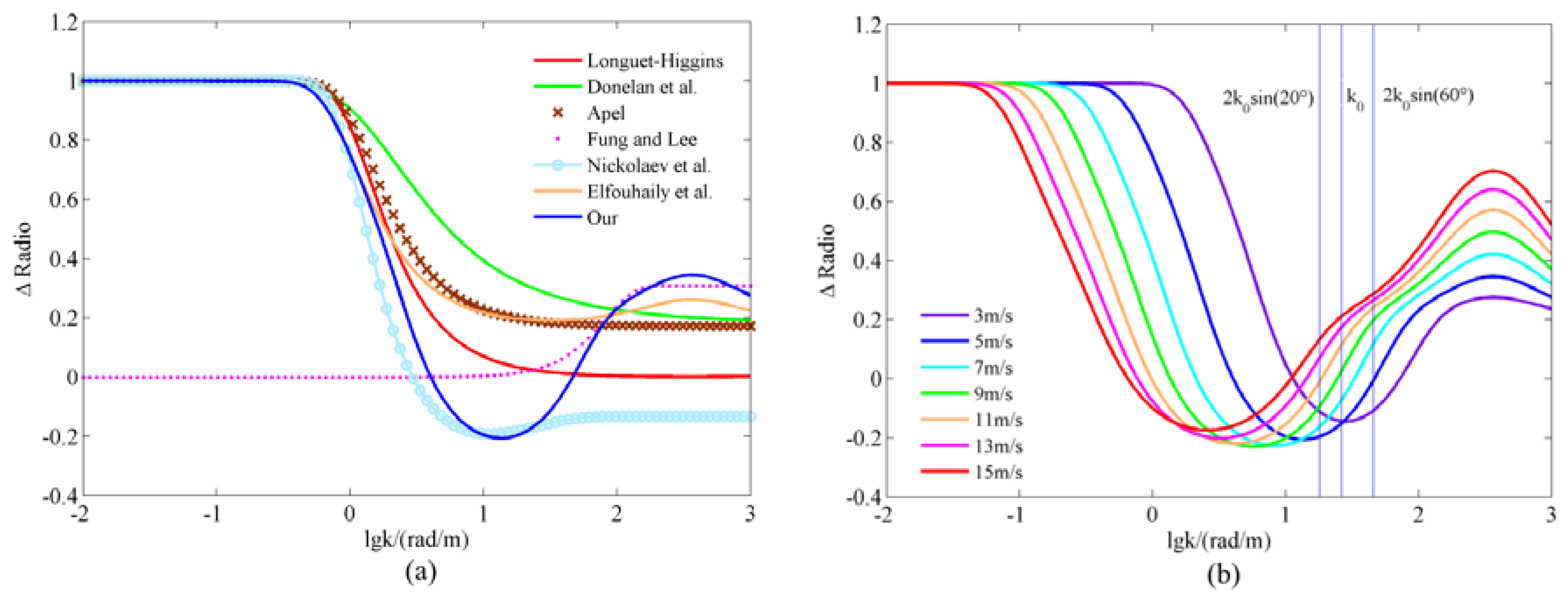
Figure 3.
Numerical curves of two angular spreading functions in polar coordinates at 5 m/s wind speed, versus wavenumber k. The upper row represents Elfouhaily ASF, and the bottom row represents our ASF. (a) Elfouhaily ASF, 0.1, 0.5, and 1 rad/m wavenumber; (b) Elfouhaily ASF, 5, 10, and 50 rad/m wavenumber; (c) Elfouhaily ASF, 100 and 500 rad/m wavenumber; (d) Our ASF, 0.1, 0.5, and 1 rad/m wavenumber; (e) Our ASF, 5, 10, and 50 rad/m wavenumber; (f) Our ASF, 100 and 500 rad/m wavenumber.
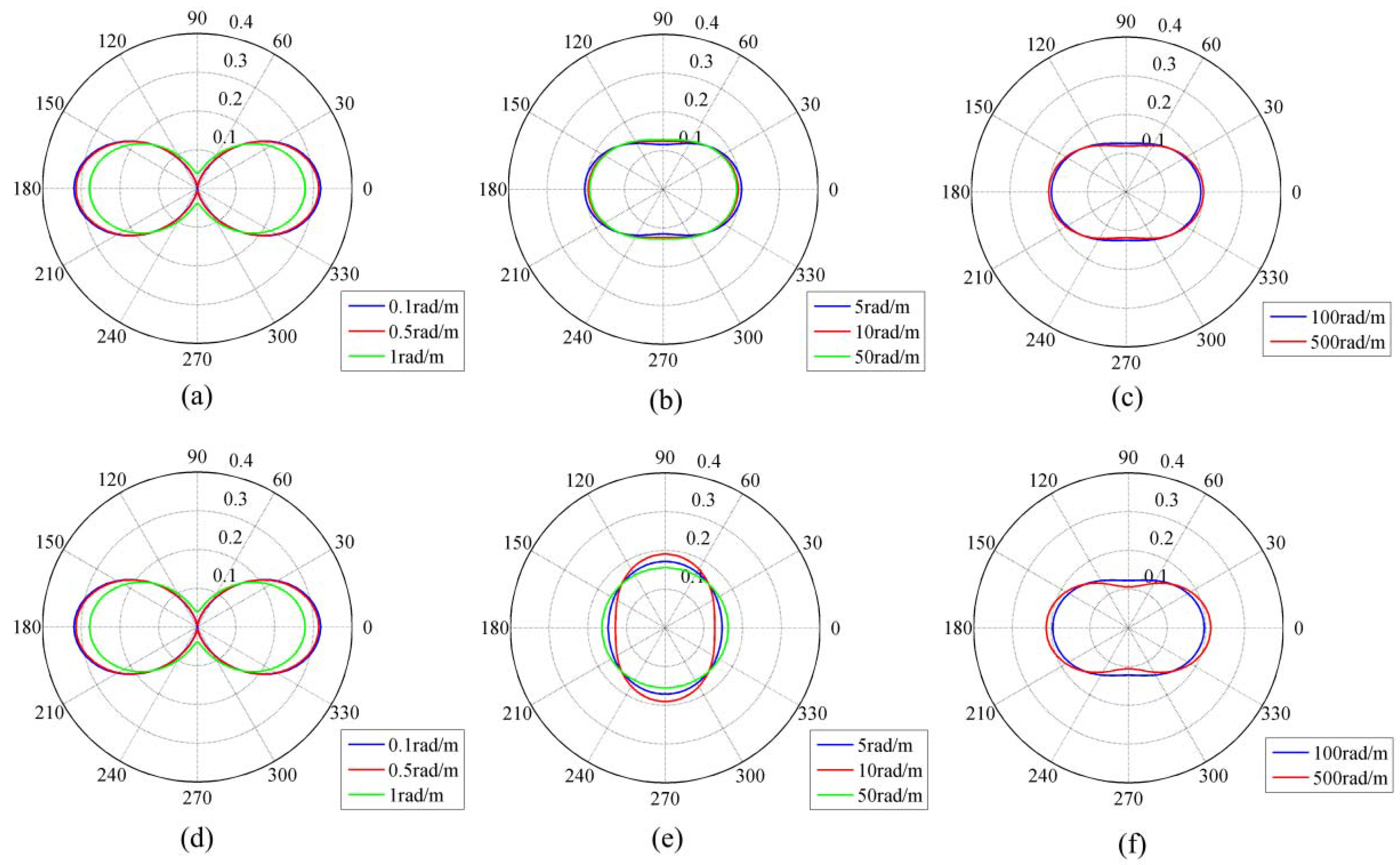
Figure 4.
Comparison of normalized radar backscattering cross-sections (NRCSs) from model simulations and satellite observations versus relative wind direction. Each row represents a different wind speed; i.e., 3, 5, 8, 10, 12, 15 m/s. In each wind speed panel, the left column corresponds to beam 1, the middle column corresponds to beam 2, and the right column corresponds to beam 3. Here, beams 1, 2 and 3 denote the incidence angles of 28.7°, 37.8° and 45.6°, respectively. Red stars and circles are the binned matchup averages for VV and HH polarization, respectively; the vertical bars represent of the matchup data. Blue dashed lines and solid lines are model simulations for VV and HH polarization, respectively.
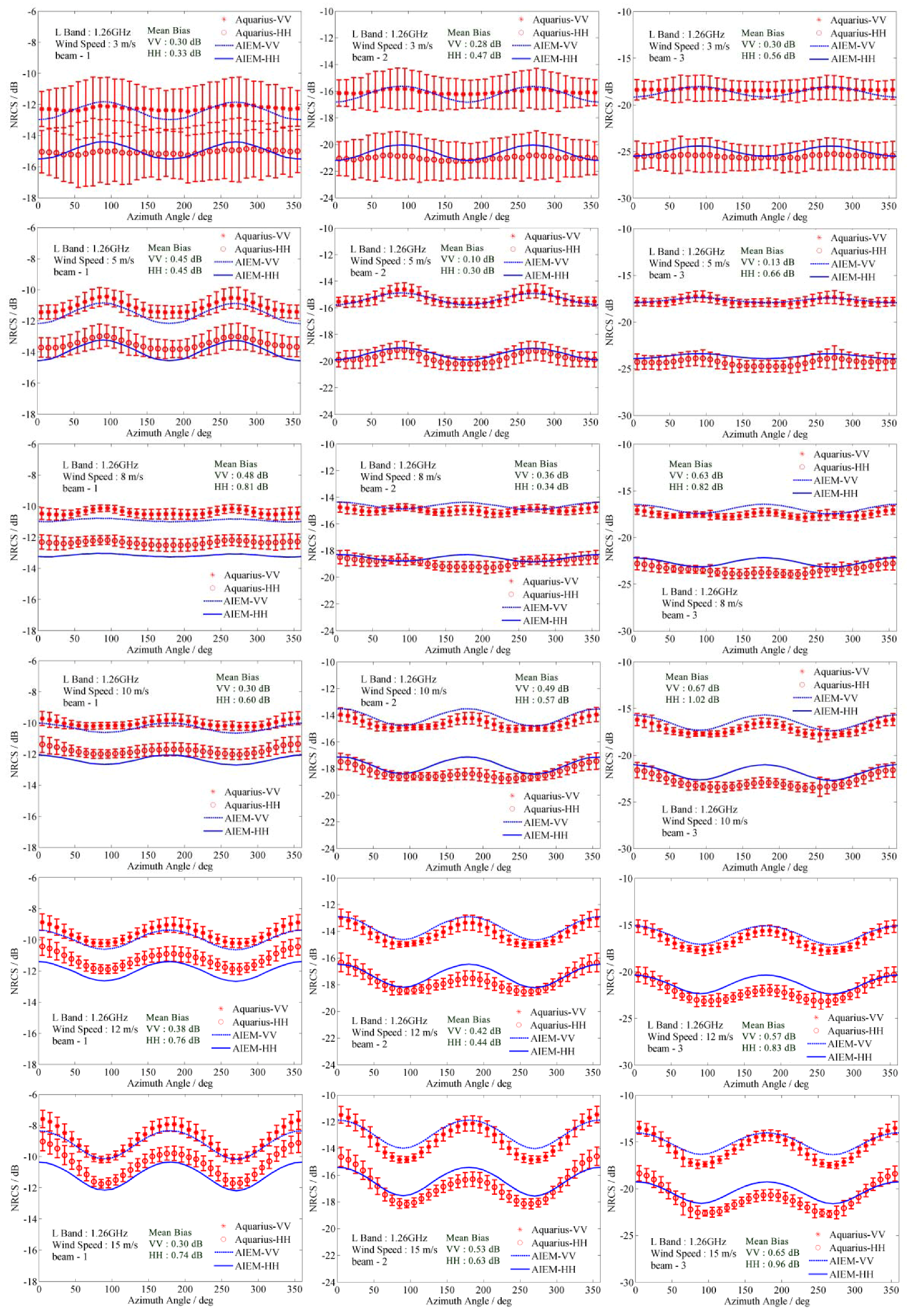
Figure 5.
Comparison of azimuthal features of scattering curves between model simulations with two ASFs and satellite observations. The upper and bottom rows represent the wind speed at 5 and 12 m/s wind, respectively. The left column corresponds to beam 1, the middle column corresponds to beam 2, and the right column corresponds to beam 3. Here, beams 1, 2 and 3 denote the incidence angles of 28.7°, 37.8° and 45.6°, respectively. Red stars and circles are the binned matchup averages for VV and HH polarization, respectively; the vertical bars represent of the matchup data. Dash lines and solid lines are model simulations for VV and HH polarization, respectively. Green and blue lines denote the model simulations with Elfouhaily’s ASF and our improved ASF, respectively.
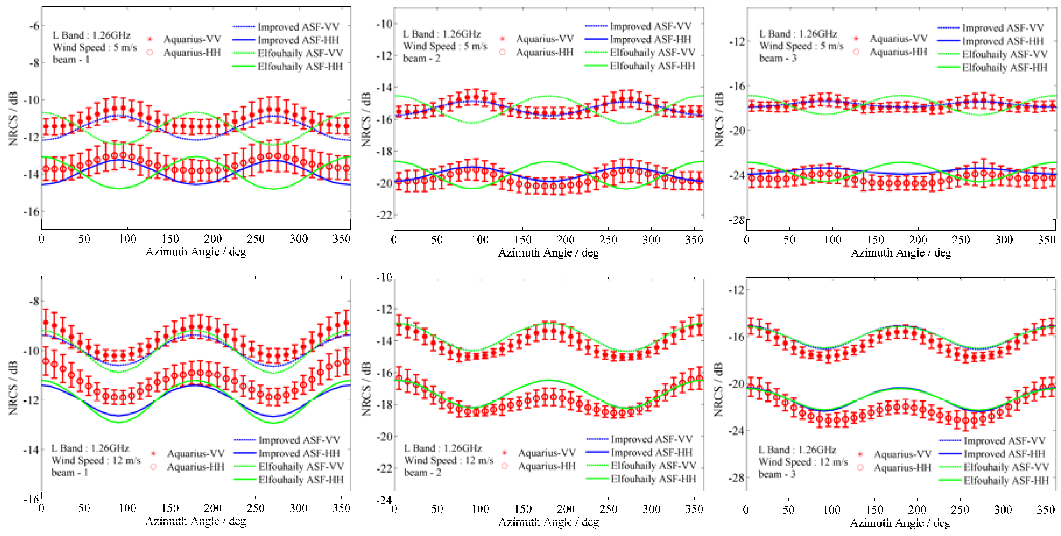
Figure 6.
The upper and middle rows show a comparison of NRCSs from model simulations with different ASFs and satellite observations versus wind speed in the upwind and crosswind direction, respectively. The left column corresponds to beam 1, the middle column corresponds to beam 2, and the right column corresponds to beam 3. Here, beam 1, 2 and 3 denote the incidence angles of 28.7°, 37.8° and 45.6°, respectively. Red stars and circles are the binned matchup averages for VV and HH polarization, respectively; vertical bars represent of matchup data. Dashed lines and solid lines are model simulations for VV and HH polarization, respectively. Green and blue lines denote the model simulations with Elfouhaily’s ASF and our improved ASF, respectively. The bottom row shows the number of data points for calculations at each beam.

Figure 7.
Comparison of Δ radio and Δ′ calculated by Aquarius observations versus wind speeds at L-band. Red dash lines with stars are Δ′ calculated in liner scale with Aquarius observations. Blue solid lines with open circles are Δ radios of our ASF. (a) Beam 1; (b) Beam 2; (c) Beam 3.
Figure 7.
Comparison of Δ radio and Δ′ calculated by Aquarius observations versus wind speeds at L-band. Red dash lines with stars are Δ′ calculated in liner scale with Aquarius observations. Blue solid lines with open circles are Δ radios of our ASF. (a) Beam 1; (b) Beam 2; (c) Beam 3.
© 2017 by the authors. Licensee MDPI, Basel, Switzerland. This article is an open access article distributed under the terms and conditions of the Creative Commons Attribution (CC BY) license (http://creativecommons.org/licenses/by/4.0/).
Share and Cite
MDPI and ACS Style
Du, Y.; Yang, X.; Chen, K.-S.; Ma, W.; Li, Z. An Improved Spectrum Model for Sea Surface Radar Backscattering at L-Band. Remote Sens. 2017, 9, 776. https://doi.org/10.3390/rs9080776
AMA Style
Du Y, Yang X, Chen K-S, Ma W, Li Z. An Improved Spectrum Model for Sea Surface Radar Backscattering at L-Band. Remote Sensing. 2017; 9(8):776. https://doi.org/10.3390/rs9080776
Chicago/Turabian StyleDu, Yanlei, Xiaofeng Yang, Kun-Shan Chen, Wentao Ma, and Ziwei Li. 2017. "An Improved Spectrum Model for Sea Surface Radar Backscattering at L-Band" Remote Sensing 9, no. 8: 776. https://doi.org/10.3390/rs9080776
Note that from the first issue of 2016, this journal uses article numbers instead of page numbers. See further details here.