Application of Abundance Map Reference Data for Spectral Unmixing


Chester F. Carlson Center for Imaging Science, Rochester Institute of Technology, Rochester, NY 14623, USA
*
Author to whom correspondence should be addressed.
Remote Sens. 2017, 9(8), 793; https://doi.org/10.3390/rs9080793
Submission received: 13 June 2017
/
Revised: 19 July 2017
/
Accepted: 27 July 2017
/
Published: 1 August 2017
Abstract
:Reference data (“ground truth”) maps have traditionally been used to assess the accuracy of classification algorithms. These maps typically classify pixels or areas of imagery as belonging to a finite number of ground cover classes, but do not include sub-pixel abundance estimates; therefore, they are not sufficiently detailed to directly assess the performance of spectral unmixing algorithms. Our research aims to efficiently generate, validate, and apply abundance map reference data (AMRD) to airborne remote sensing scenes. Scene-wide AMRD for this study were generated using the remotely sensed reference data (RSRD) technique, which spatially aggregates classification or unmixing results from fine scale imagery (e.g., 1-m GSD) to co-located coarse scale imagery (e.g., 10-m GSD or larger). Validation of the accuracy of these methods was previously performed for generic 10 m × 10 m coarse scale imagery, resulting in AMRD with known accuracy. The purpose of this paper was to apply this previously validated AMRD to specific examples of airborne coarse scale imagery. Application of AMRD involved three main parts: (1) spatial alignment of coarse and fine scale imagery; (2) aggregation of fine scale abundances to produce coarse scale imagery specific AMRD; and (3) demonstration of comparisons between coarse scale unmixing abundances and AMRD. Spatial alignment was performed using our new scene-wide spectral comparison (SWSC) algorithm, which aligned imagery with accuracy approaching the distance of a single fine scale pixel. We compared simple rectangular aggregation to coarse sensor point-spread function (PSF) aggregation, and found that PSF returned lower error, but that rectangular aggregation more accurately estimated true AMRD at ground level. We demonstrated various metrics for comparing unmixing results to AMRD, including several new techniques which adjust for known error in the reference data itself. These metrics indicated that fully constrained linear unmixing of AVIRIS imagery across all three scenes returned an average error of 10.83% per class and pixel. Our reference data research has demonstrated a viable methodology to efficiently generate, validate, and apply AMRD to specific examples of airborne remote sensing imagery, thereby enabling direct quantitative assessment of spectral unmixing performance.
1. Introduction
Reference data maps, which are often called “ground truth” maps in remote sensing literature [1,2], are maps that accurately label areas or pixels of the map as belonging to a finite number of ground cover classes. Such maps have traditionally been used to assess the accuracy of classification algorithms. Well known examples of reference data (RD) include Cuprite [3], Indian Pines [4], Salinas [5], and Pavia [6]. These pixel-wise RD have been used extensively to quantitatively evaluate the performance of classification algorithms. Abundance map reference data (AMRD) are a special type of RD, where each pixel is allowed to be a mixture of the various ground cover classes. AMRD are designed to quantitatively evaluate the performance of spectral unmixing algorithms [7,8]. However, we are not aware of any similarly well-known and widely-available AMRD scenes for airborne imaging spectrometer (IS) data.
Traditional methods of generating RD, such as field surveys and imagery analysis, have not been undertaken frequently because of the time and expense required to accurately generate such data [9]. The added complexity of allowing each RD pixel to be a mixture of the various ground cover classes further complicates the problem. In order to efficiently generate scene-wide AMRD, we proposed a technique called remotely sensed reference data (RSRD) [7], which creates AMRD for coarse scale imagery using co-located fine scale imagery. Specifically, RSRD performs standard classification or unmixing on fine scale imagery (e.g., 1-m GSD National Ecological Observatory Network (NEON) IS), then aggregates fine scale results to co-registered coarse scale pixels (e.g., 15-m GSD Airborne Visible/Infrared Imaging Spectrometer (AVIRIS) IS), thereby creating AMRD for the coarse scale imagery. RSRD methodology is similar to previous studies which have created sub-pixel RD using high-resolution RGB videography [10], RGB imagery [11], multi-spectral imagery [12], and IS imagery [13,14,15].
While RD frequently have been used to assess the performance of classification algorithms and occasionally have been used to assess unmixing algorithms, many studies neglect to account for the accuracy of the RD itself. This means that RD of unknown accuracy often have been used as the benchmark for assessing the accuracy of other algorithms. Indeed, we are not aware of any RD scenes with published validation studies of the RD itself.
In order to determine the accuracy of AMRD generated using the RSRD technique, we conducted an extensive validation study of AMRD for three remote sensing scenes [8]. This paper continues our work with AMRD by applying our previously generated and validated AMRD to specific coarse scale airborne IS imagery. The main concepts involved in applying validated AMRD to coarse scale imagery are listed below.
- Spatial alignment of fine and coarse scale imagery
- Aggregation of fine scale abundances to produce specific coarse scale AMRD
- Comparison of spectral unmixing results and AMRD.
The objective of this study, therefore, is to implement these main concepts using several versions of coarse scale imagery and spectral unmixing. The subsequent sections introduce these important concepts in more detail.
1.1. Spatial Alignment
Accurate spatial alignment between fine and coarse scale imagery is necessary to properly use validated AMRD. Misalignment by only half a coarse scale pixel would significantly increase the error in AMRD itself. Imprecise spatial alignment would necessitate scaling analysis to multiple pixel windows, for example, one previous study using RSRD-like RD recommended scaling analysis to 9 × 9 Landsat pixel windows (270 m × 270 m on the ground) due to inaccurate alignment between fine and coarse imagery [10].
Airborne imagery georegistration is often accurate to 0.5–1.0 pixels. For example, AVIRIS does not claim sub-pixel accuracy from their improved (2010 version) orthorectification and georeferencing processing [16]. We have observed registration errors of 15+ m between NEON and AVIRIS imagery [7]. Lack of georeferencing accuracy necessitates image-to-image spatial alignment, rather than relying on imaging system geocoding.
Image registration is a vast field of research where numerous approaches and algorithms have been developed for a wide variety of image processing tasks. Common approaches include feature matching and intensity correlation, with comparisons made in both the spatial and frequency domains, while post registration resampling and alignment of data are carried out with affine transforms or warping [17]. Remote sensing image registration has often relied on feature matching methods and warping [18,19]. It should be noted that image registration for RSRD is challenging due to highly dissimilar spatial resolution, the need for sub-pixel registration accuracy, and the use of different imaging sensors.
Spatial Fidelity of Individual Coarse Pixels
In addition to aligning fine and coarse scale imagery at the whole scene level, we must also concern ourselves with the spatial fidelity of individual coarse pixels. Much processing occurs between initial airborne collection of radiometric information and final output of imagery, which often includes atmospheric compensation, ortho-rectification, resampling to a north-south oriented grid, etc. [1,2,20]. The method used to spatially resample imagery is of special importance to the spatial fidelity of individual coarse pixels. Nearest-neighbor resampling is often employed in the ortho-rectification and resampling to a north-south grid process [21,22], prioritizing the radiometric fidelity of each collected sample, rather than the spatial fidelity of radiometric information. In the best case, nearest-neighbor resampling results in some final pixels whose reflectance values are a result of initial collections at pixel edge rather than at pixel center. In the worst case, nearest-neighbor resampling results in significant pixel re-use, where adjacent pixels are identical, because one airborne collection sample was spatially closest to two or more final pixels.
1.2. Spatial Aggregation
Aggregation is the term we use to describe averaging together the spectra of many fine pixels that are co-located within a single coarse scale pixel. Aggregation can be implemented using a simple averaging filter covering the rectangular area conceptualized by each coarse scale pixel, or it can take into account the point spread function (PSF) of a pixel, where reflected light from the center of pixels contributes more to the final reflectance value of a pixel than light from pixel edges, and at the same time, each pixel is affected by reflected light originating from outside its rectangular pixel outline [23,24]. The rectangular method is more representative of cover class mixtures on the ground, while the later is more representative of the radiometric information that would have been collected by the imaging sensor. Both methods are used in this study for purpose of comparison.
1.3. Comparison of Unmixing Results and AMRD
In most cases, AMRD have not been available to quantitatively assess the performance of spectral unmixing algorithms. In the absence of AMRD, researchers have used various methods to assess performance. Qualitative assessments have visually compared unmixing results to well-known RD, such as Cuprite, Indian Pines, and Pavia [25,26,27]. Quantitative assessments have used synthetic data [25,26,27], average per-pixel residual error [27,28], used the mean of several algorithms as the ideal and computed residuals from the ideal [28], etc.
Confusion matrices have been the standard method of quantitative comparison between RD maps and classification algorithms [1,2,9]. A confusion matrix is an matrix for an n-class problem. Rows of the matrix typically represent RD, while columns represent classification data, where the th entry represents the number of pixels in the image belonging to class-i that were classified to class-j. Confusion matrices allow the evaluation of overall classification accuracy, as well as providing insight into which classes tend to be confused with one another. Unfortunately, confusion matrices aren’t readily applicable to spectral unmixing and AMRD. Methods have been proposed to generalize confusion matrices for use with AMRD [29], but these methods do not allow straight-forward comparison of individual matrix elements, and essentially amount to comparing total RD area to total unmixed area per class.
As mentioned previously, there are a number of studies that have produced sub-pixel RD through methodologies similar to our RSRD process. These studies also implemented methods to compare AMRD with spectral unmixing results, with the most common strategy being calculation of mean absolute error (MAE) and/or root-mean square error (RMSE) [11,12,13]. Several studies plotted unmixed fraction versus RD fraction and computed a linear regression of the result. Using this technique, perfect unmixing would result in an and slope equal to unity, with the intercept equal to zero [10,13].
2. Methodology
2.1. Data
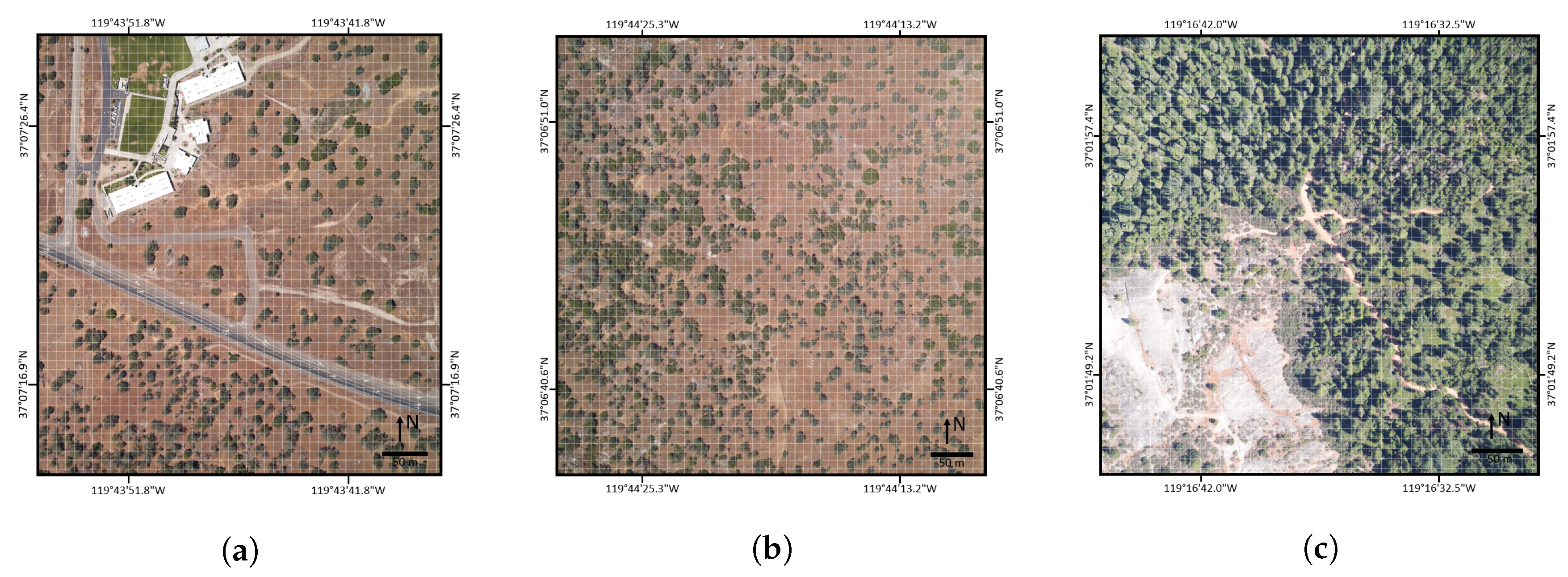
The three study scenes used in this paper are located on or near NEON Domain 17 (D17) research sites near Fresno, CA, USA. We selected these specific areas because they contained significant ground cover variation. The three scenes contain mostly natural landscapes, including high mountain forests, large rock outcroppings, dry valley grasslands, and oak savannah. We also included a developed area with buildings, roads, grass fields, etc. These cover types are representative of many remote sensing scenes and the results should be generally applicable to other similar studies. Extension of our methodologies to more complex urban landscapes should be possible, but we caution that each additional ground cover class increases the complexity of reference data generation and validation, while likely lowering the accuracy of resulting AMRD. Further information for each site is listed below and RGB imagery of the study areas is shown in Figure 1.
- SJERHS—San Joaquin Experimental Range (SJER), Minarets High School (HS)—Located just outside the northern extent of SJER land on privately owned Minarets High School property.
- SJER116—San Joaquin Experimental Range (SJER), NEON field site 116—Located on public property in the area surrounding NEON SJER field site #116.
- SOAP299—Soaproot (SOAP) Saddle, NEON field site 299—Located on public property in the area surrounding NEON SOAP field site #299.
NEON and AVIRIS conducted a joint aerial campaign over these areas in June 2013. Table 1 contains detailed information on the imagery provided to us by NEON and AVIRIS, along with synthetic coarse scale imagery (NEON 15 m/29 m), which we used in this experiment. NEON RGB data were not used in processing tasks, but were useful for enhancing human analyst understanding of the study areas. Note that we used both orthorectified and unorthorectified AVIRIS data in this study, because AVIRIS’ orthorectification processing resulted in many replicated pixels due to nearest-neighbor resampling.
AVIRIS Ortho data were generated as part of the NASA HyspIRI preparatory campaign, which spatially resampled data to a 15-m GSD grid, rather than the standard 18-m GSD grid. This finer sample spacing resulted in higher than normal pixel reuse from nearest-neighbor resampling. Figure 2 displays the amount of pixel reuse in AVIRIS Orthorectified vs AVIRIS Unorthorectified data for the SJERHS scene. This trend was present in all three scenes.
We generated synthetic coarse scale imagery from NEON IS data via frequency domain filtering and spatial domain downsampling of fine scale data using a Gaussian filter, whose spatial domain full width at half maximum (FWHM) was equal to the desired final GSD, thereby simulating coarse sensor PSF. We used this method to create NEON 15 m and NEON 29 m data. The NEON 15 m data were introduced for purposes of comparison with AVIRIS Ortho and Unortho data, while the NEON 29 m data were introduced to study the implications of applying our validated AMRD to coarser scale imagery.
2.2. Validated Abundance Map Reference Data
As mentioned previously, the primary purpose of this paper is to demonstrate the application of previously validated AMRD to specific examples of airborne remotely sensed imagery, such as the AVIRIS imagery described in Table 1. We recommend reviewing the validation paper [8] for detailed information on the validation process; however, we will mention the effort briefly here.
Let be an estimate of , using method m, where is the “true” abundance fraction of ground cover class c in coarse pixel p. We generated for 10 m × 10 m plots, randomly chosen from the three study scenes, ground cover classes, and independent methods of abundance estimates. Details of C and M are listed below. As discussed previously, RSRD aggregates fine scale classification or unmixing results to co-located coarse scale pixels, thereby estimating abundance fractions. We performed the underlying classification/unmixing using a Euclidean distance (ED) classifier, non-negative least squares (NNLS) spectral unmixing algorithm, and by taking the posterior probabilities from a maximum likelihood (ML) estimator, thereby estimating coarse scale abundances using independent algorithms employed within the RSRD framework.
- : Photosynthetic Vegetation (PV)
- : Non-Photosynthetic Vegetation (NPV)
- : Bare Soil (BS)
- : Rock
- : Field surveys by Observer-A (Field-A)
- : Field surveys by Observer-B (Field-B)
- : Imagery analysis by Observer-A on NEON IS, aided by NEON RGB (Analyst-A)
- : Imagery analysis by Observer-B on NEON IS, aided by NEON RGB (Analyst-B)
- : RSRD by Euclidean distance (ED) on NEON IS (RSRD-ED)
- : RSRD by non-negative least squares (NNLS) spectral unmixing on NEON IS (RSRD-NNLS)
- : RSRD by maximum likelihood (ML) on NEON IS (RSRD-ML)
We found statistically significant differences between , , … , , and concluded that no single estimate method was demonstrably superior, based on pairwise comparisons. Given that was unknown, we concluded that the best estimate of true abundance fractions within each 10 m × 10 m plot was the mean of all (MOA) independent versions. MOA is defined in Equation (1).
We then compared each estimation method to MOA using Equations (2)–(4), and found that (Analyst-B) was the closest method to MOA; however, (RSRD-NNLS) was nearly as close to MOA, and provided the opportunity to efficiently generate scene-wide AMRD. As such, we selected RSRD-NNLS to serve as AMRD for our three scenes, with validated accuracy documented in Table 2. Note that we used our NNLS unmixing algorithm on fine scale imagery, but we later enforced a sum-to-one constraint on coarse scale AMRD pixels.
This validation was performed for generic 10 m × 10 m coarse scale imagery, such that the validated scenes could be applied to any co-located coarse scale imagery with GSD > 10 m, such as the AVIRIS data used in this study. The validation study suggested that further aggregation beyond 10 m GSD would decrease the expected standard deviation differences from MOA, but would have no expected effect on mean differences from MOA. Since the coarse data used in this study have GSD ≥ 15 m, we expect the resulting AMRD accuracy to be similar to that listed in Table 2, with slightly reduced standard deviation.
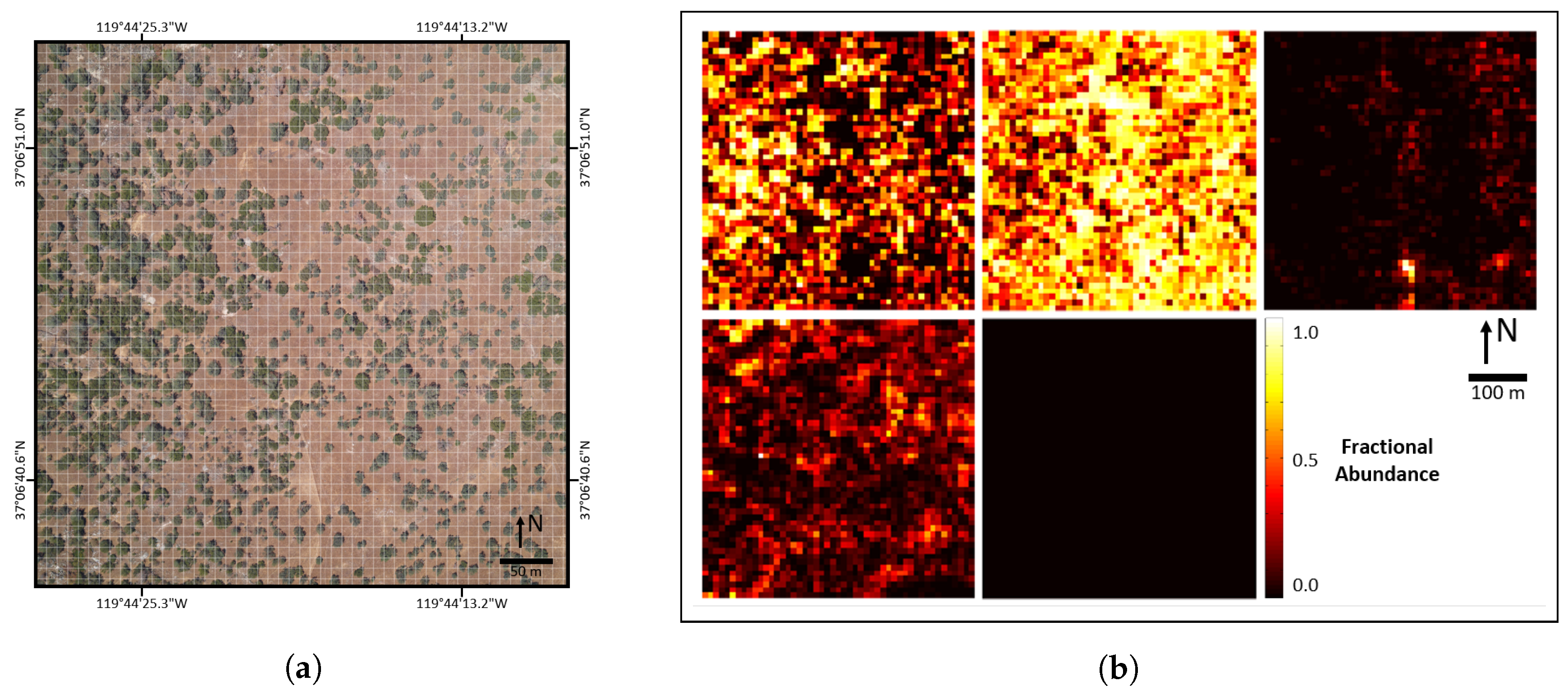
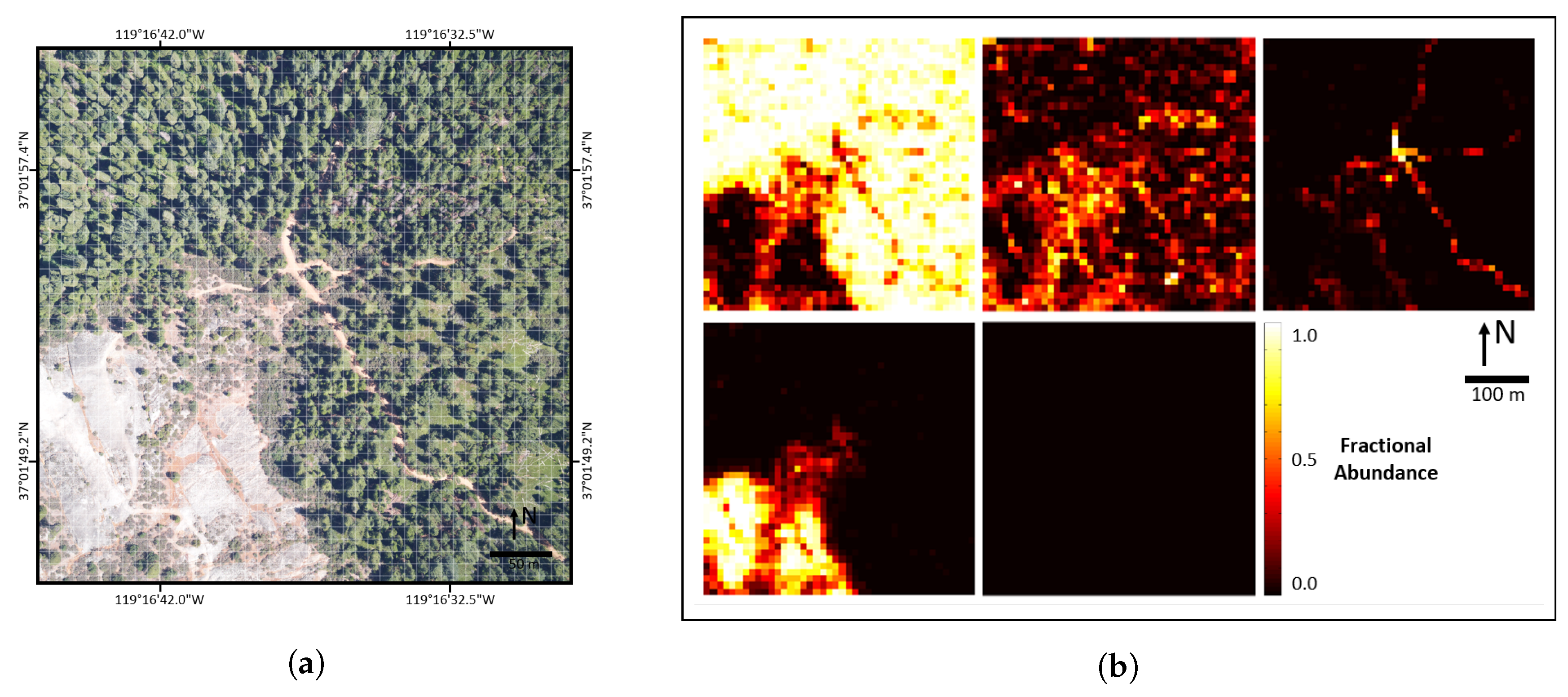
The three scenes and corresponding validated AMRD are shown in Figure 3, Figure 4 and Figure 5. Note that a fifth class, other (roof), was included in the abundance maps to account for the buildings in SJERHS. However, this class was excluded from analysis in the validation because we were not able to collect field survey validation samples on roof tops. We have also excluded it from analysis in this paper, since its accuracy was not validated.
2.3. Spatial Alignment
Spatially aligning fine scale NEON IS data and coarse scale AVIRIS IS data was an important step in applying validated AMRD to specific coarse scale imagery. We first attempted the image registration task using well known feature matching algorithms, including various configurations of ENVI’s image registration workflow [19] and a Scale-Invariant Feature Transform (SIFT) based algorithm [30]. In all cases, is was difficult to accurately identify matching features between fine and coarse scale imagery, leading to badly warped and misaligned output data. Furthermore, these algorithms resampled the warp image to coincide with the base image coordinate system, and did not provide a method to estimate registration accuracy in terms of distance on the ground. It is worth noting that the purpose of this study was not to optimize a state-of-the-art image registration algorithm; we simply needed a method capable of aligning fine and coarse scale imagery within a fraction of coarse scale pixels, thereby preserving the accuracy of validated AMRD.
As such, we used an enhanced version of our own image alignment algorithm [7] to align NEON IS imagery with AVIRIS Ortho, AVIRIS Unortho, NEON 15 m, and NEON 29 m data. We coined this algorithm as “Scene-Wide Spectral Comparison” (SWSC). SWSC is an intensity comparison, spatial domain, affine transform class alignment algorithm that uses the full spectrum of IS data for alignment comparisons. Specifically, the algorithm iteratively rotates, scales, and translates scale imagery, and at each iteration, compares coarse scale pixel spectra to an aggregation of the underlying fine scale pixel spectra. Comparisons were made using Spectral Angle Mapper (SAM) [1], which is described in Equation (5), where s represents an AVIRIS pixel spectrum and x represents an aggregation of underlying NEON pixel spectra.
The following steps detail our use of the SWSC algorithm to align NEON and AVIRIS imagery:
- Extract study scene imagery from flight-line imagery in such a way that AVIRIS scenes are larger than NEON scenes in terms of real distance on the ground.
- Spectrally resample NEON data to match AVIRIS spectral sampling, using a Gaussian model with FWHM equal to band spacing.
- Trim NEON and AVIRIS data, resulting in square study scenes with an odd number of pixels along each edge. AVIRIS should still be larger than NEON in real ground distance.
- Construct an x-y coordinate system for each image, where the image center is located at the origin and each pixel is represented by an integer value.
- Compute the mean of all comparisons in the previous step.
- Cycle through all rotation, scale, and translation iterations.
- Examine the mean graphs to identify the rotation, scale, and translation position resulting in the minimum mean , this is the location of optimal alignment.
- Based on the optimal alignment location, trim excess AVIRIS and NEON imagery, resulting in final aligned images.
- Based on the optimal alignment location, aggregate validated AMRD corresponding to final aligned AVIRIS imagery, resulting in final aligned AVIRIS specific AMRD.
- Confirm alignment via visual inspection of imagery and AMRD.
When aligning data, we first defined a range of possible parameters for rotation, scale, and translation via visual inspection of imagery. We then ran steps 5–8 of the algorithm described above several times, each time narrowing parameter ranges and sampling distances. This manual optimization of alignment parameters could likely be automated in the future to improve algorithm usability. Imagery was considered aligned when mean graphs showed well-defined troughs and parameter sampling distances had reached the following precision:
- Rotation: 1/10 Degree
- Scale: 1/100 Multiplication
- Translation: 1 Single Fine Scale Pixel
This sampling precision resulted in approximately single fine scale pixel precision at imagery edges, from each parameter. The combined precision error from the three parameters, along with uncertainty in mean graphs, could result in an absolute spatial alignment error greater than one fine pixel, with the error expected to increase toward imagery edges.
2.4. Spatial Aggregation
Aggregation of fine scale pixels corresponding to coarse scale pixels was used in both the SWSC algorithm and in subsequent generation of final coarse scale AMRD. We performed both these tasks using two versions of aggregation, a simple rectangular averaging filter the size of coarse scale pixels, and a Gaussian filter with full width half max (FWHM) equal to the GSD of coarse scale pixels. Gaussian aggregation of fine scale pixels was representative of the coarse scale sensor PSF [20]. Rectangular aggregation was performed via averaging pixel spectra in the spatial domain, while PSF aggregation was performed via multiplication in the frequency domain and downsampling in the spatial domain.
2.5. Spectral Unmixing
Spectral unmixing of coarse imagery was performed in order to demonstrate assessment of unmixing performance using AMRD. We unmixed the coarse scale imagery using unconstrained least squares (LS) [1], non-negative least squares (NNLS) [31], and fully-constrained least squares (FCLS) [31], represented by Equations (10)–(12), respectively. We re-used the same endmembers for coarse scale unmixing that we had used to produce our validated AMRD. In the case of AVIRIS Ortho/Unortho unmixing, NEON derived endmembers were spectrally resampled to match AVIRIS bands. Endmembers were obtained from NEON IS imagery by manual inspection and selection, including choosing ten exemplar pixels for each initial ground cover class, whose spectral mean served as the class endmember (). While this method was somewhat simplistic compared to state of the art endmember generation and variability research, its accuracy compared to field surveys and imagery analysis was carefully validated in our previous work. Endmembers were selected independently for each of the three scenes and remained constant throughout validation and application. Unmixing was performed using a larger number of initial ground cover classes, which were subsequently combined into our final ground cover classes of PV, NPV, BS, and Rock. For example, in the SJERHS scene, initial ground cover classes were: white roof, grey roof, grass vegetation, tree vegetation, dry vegetation, dry grass, dirt road, dirt trail, concrete, and blacktop. We selected these initial ground cover classes to characterize the major spectral variation within the scene. Unmixing was performed using these initial ground cover classes, with resulting abundances being combined to produce abundances for our final cover classes. Further details are available in our AMRD validation paper [8].
2.6. Comparison of Spectral Unmixing Results and AMRD
Previous methods of comparing spectral unmixing abundances to AMRD include mean absolute error (MAE), root-mean square error (RMSE), and linear regression. In this study, we compared spectral unmixing abundance maps to AMRD using the previously introduced MAE and LR methods, along with new methods called reference data mean adjusted MAE (MA-MAE) and reference data confidence interval adjusted MAE (CIA-MAE). These new methods take into account the known error in the AMRD itself, which is listed in Table 2. While basic MAE measures error compared to AMRD, MA-MAE and CIA-MAE are more interesting because they remove mean error in the AMRD, thereby tying error estimation back to true ground abundances. The MAE-based comparisons are described in Equations (13)–(16), where are unmixing abundances, are reference data, are AMRD mean distances from MOA, and are AMRD confidence intervals.
The regression comparison methods are described in Equations (17)–(19), where Equation (17) is solved using simple linear regression to obtain the slope and intercept . The calculated abundances, , are found using Equation (18), and the closeness of fit, , is found using Equation (19), where represents the mean unmixing fraction of class c.
3. Results
3.1. Spatial Alignment Accuracy
Spatial alignment was performed between NEON IS imagery and AVIRIS Ortho, AVIRIS Unortho, NEON 15 m, and NEON 29 m imagery for the SJERHS, SJER116, and SOAP299 scenes using Scene Wide Spectral Comparison (SWSC). SWSC alignment depended on identifying the rotation, scale, and translation parameters corresponding to the minimum mean between coarse and fine scale imagery.
Figure 7 displays an example of the mean graphs we used to identify rotation, scale, and translation parameters for optimal spatial alignment. This particular case is from alignment of NEON IS and AVIRIS Unortho imagery for the SJERHS scene. As Figure 7a indicates, the troughs for scale were less smooth and well behaved than rotation and translation troughs, when all troughs were zoomed to a range equal to 100× the precision required for 1 m alignment accuracy at image edge.
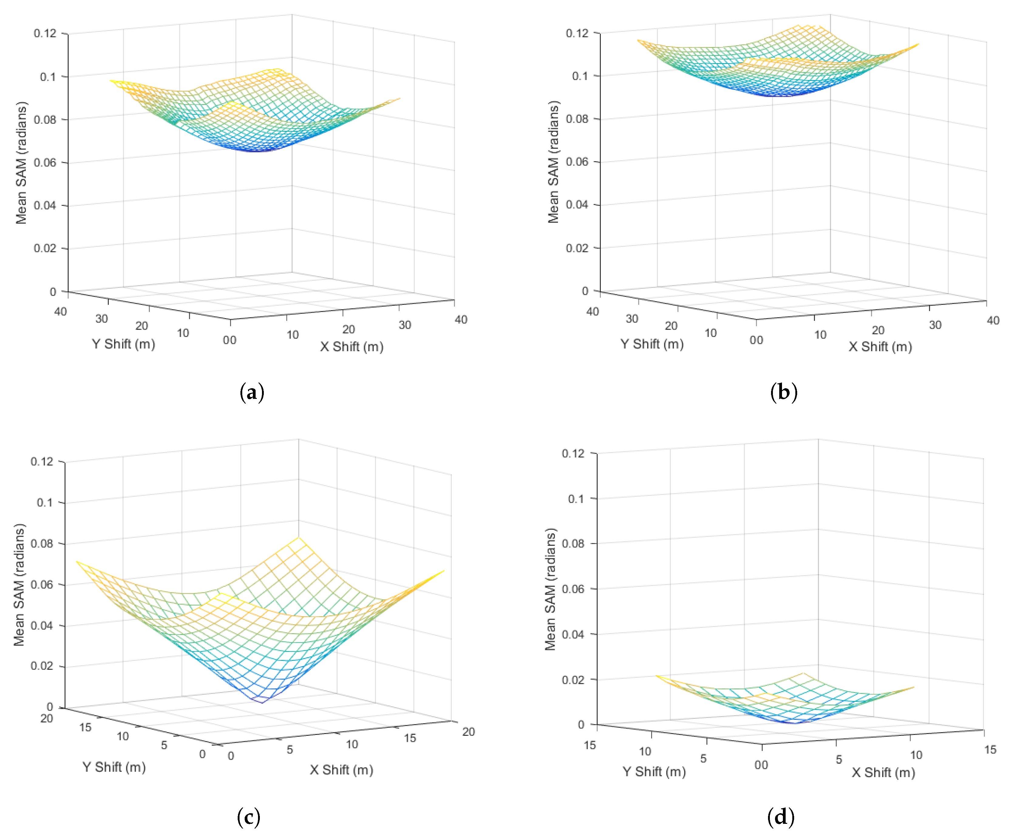
Figure 8 displays the translation parameter’s mean troughs for AVIRIS Ortho, AVIRIS Unortho, NEON 15 m, and NEON 29 m. We chose the same vertical scale for all sub-figures in order to more easily compare the relative mean ranges for the various versions of coarse imagery. Mean values were significantly lower for the semi-synthetic coarse imagery, i.e., NEON 15 m and 29 m, than for the AVIRIS coarse imagery. Surprisingly, mean values for AVIRIS Ortho were lower than AVIRIS Unortho, despite the high rate of pixel reuse from nearest-neighbor resampling.
Table 3 lists the minimum mean values between NEON SI and all four versions of coarse imagery, using both PSF and rectangular aggregation, for the SJERHS, SJER116, and SOAP299 scenes. In general, mean values were lowest for the SJERHS scene and highest for the SOAP299 scene. We attributed these differences in alignment accuracy to steep elevation gradients and shade shifting throughout the day in the SOAP299 scene. PSF aggregation returned slightly lower mean results than the rectangular case. Similar to the results displayed in Figure 8, alignment between NEON IS and semi-synthetic coarse imagery returned much lower mean values than alignment with AVIRIS imagery.
Occasionally, PSF and rectangular aggregation methods yielded slightly different rotation, scale, and/or translation parameters, which amounted to alignment differences of less than 1 m. In these cases, we split the difference between the results from the two methods. Since NEON 15 m/29 m data were generated directly from NEON IS data, we knew the position of correct alignment, and in all cases, the SWSC method re-aligned NEON 15 m/29 m within one fine scale pixel of the true values.
3.2. Assessing the Performance of Unmixing Using Mean Absolute Error
We computed MAE, MA-MAE, and CIA-MAE for all permutations of four image types (i, I = 4), three unmixing types (u, U = 3), and two AMRD types (r, R = 2), resulting in , , and . We then compared results within each category, by averaging across all permutations from the other categories. For example, . The results of this analysis are shown in Table 4. In this analysis, we combined results from three study scenes and four ground cover classes, due to the large amount of available data. Note that errors for certain scenes or classes may depart significantly from the mean, as shown in Figure 9.
Our semi-synthetic coarse imagery, NEON 15 m/29 m, had far lower errors than AVIRIS Ortho/Unortho data, and unexpectedly, AVIRIS Ortho had lower errors than AVIRIS Unortho. LS unmixing produced far higher errors than NNLS and FCLS unmixing. PSF aggregated AMRD yielded slightly lower errors than the rectangular case. Finally, we found that the error of MAE was lower than MA-MAE, and that MA-MAE was lower than both CIA-MAE lower and upper levels. Given the inaccuracy of LS unmixing, we recomputed image and reference type error metrics, while excluding LS unmixing, resulting in Table 5.
Table 5 confirmed most of the findings from Table 4, including that the error in NEON 15 m/29 m < AVIRIS Ortho/Unortho, PSF < Rect, MAE < MA-MAE, and MA-MAE < . However, with LS unmixing results removed, the errors in AVIRIS Ortho and Unortho were approximately the same. Also, the differences between the error in unmixing results from NEON 15 m/29 m and AVIRIS Ortho/Unortho were not as large. Large errors in unconstrained LS unmixing disproportionately affected the AVIRIS cases, especially AVIRIS Unortho. Given that the discrepancies between NEON and AVIRIS coarse imagery were also significant, we also recomputed unmixing and reference type error metrics, while including LS unmixing and excluding AVIRIS imagery, resulting in Table 6.
Table 6 confirmed the findings from Table 4 and Table 5, as well as showing that the errors from LS unmixing were lower when AVIRIS data was excluded from the analysis. While FCLS < NNLS < LS still held true, the LS results in this synthetic imagery case were closer to those from FCLS/NNLS.
Thus far, we have used MAE analysis to explore general trends when using various versions of coarse imagery, unmixing algorithms, and reference data aggregations. We noted the following trends in unmixing errors associated with the various data and methods from this analysis:
- NEON 15 m ≈ NEON 29 m AVIRIS Ortho < AVIRIS Unortho
- FCLS < NNLS LS
- PSF < Rect
- MAE < MA-MAE, and MA-MAE <
Table 7 presents specific error results for AVIRIS Unortho coarse imagery, FCLS unmixing, and rectangular aggregation of AMRD. These results are presented as an example of analysis that can be performed on unmixing abundances using AMRD. The table indicates that there was wide variation in the accuracy of different ground cover classes, including much higher error in NPV than BS. Similar tables could be produced for every combination of coarse imagery, unmixing type, and reference data type.
3.3. Assessing the Performance of Unmixing Using Regression
Linear regression between unmixing abundances and AMRD provided another method for analyzing the performance of unmixing algorithms. Figure 9 shows the result of scatter plots of unmixing abundances versus AMRD for the same data analyzed in Table 7. We combined results from all three scenes into single plots and values in order to present more data in a limited space, and to follow the same convention we’ve used throughout our research, where results from all three scenes have been considered together. We have, however, provided color coded data per scene so that the reader can compare influences from individual scenes into the final results. Regression lines and values are included on the graphs, while slope and intercept values are provided in Table 8. Regression analysis added to the understanding provided by MAE, and clarified certain findings. For example, contrary to MAE findings, regression indicated that BS may have been the least accurate class, with low MAE simply due to lower abundance in general for BS. The combined use of MAE and regression analysis improved our understanding of unmixing results.
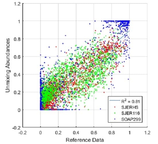
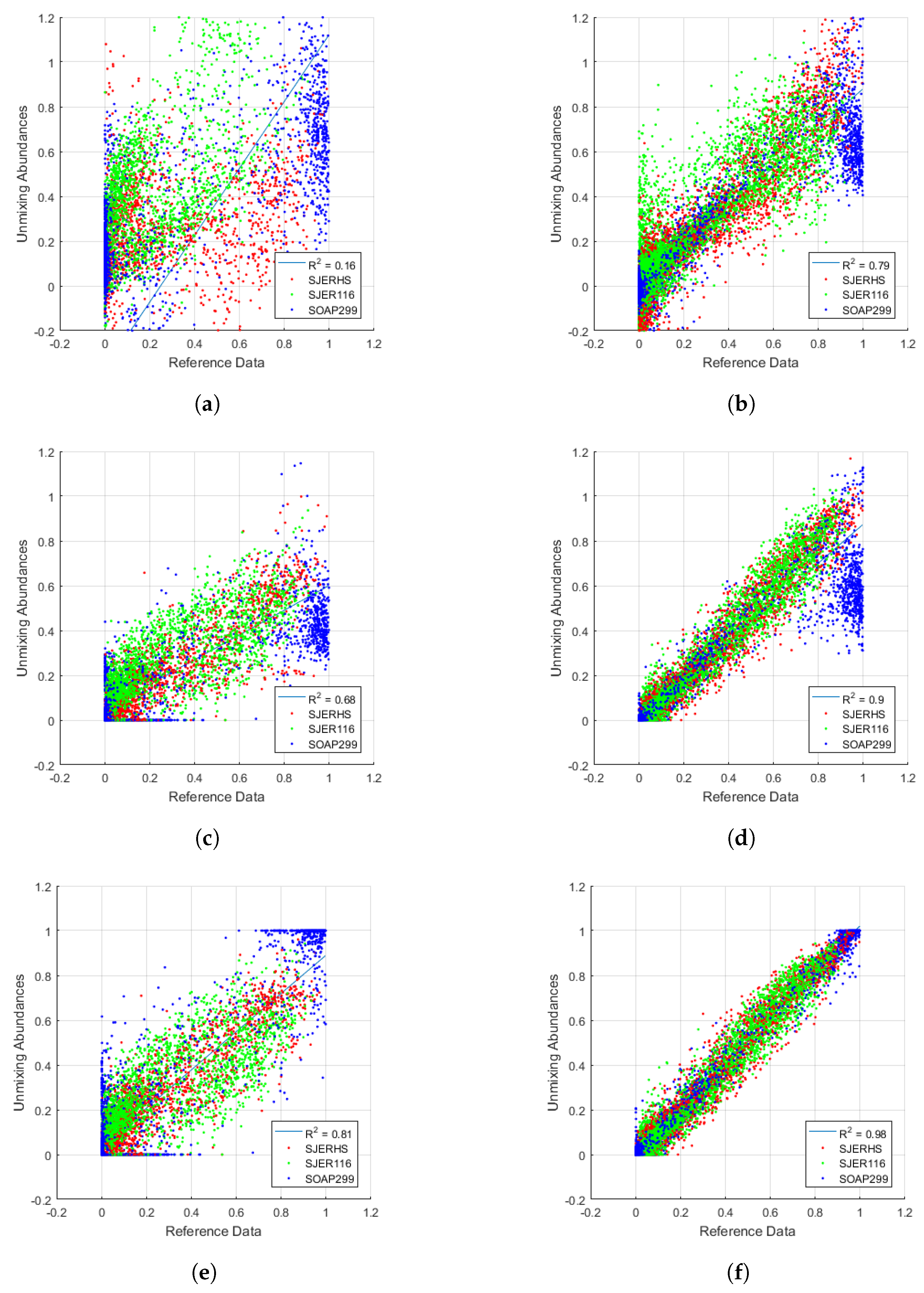
Figure 10 is similar to Figure 9, except that data from all four classes were combined into single plots, and the regression was computed for all classes combined. The left side of Figure 10 contains plots from LS, NNLS, and FCLS unmixing of AVIRIS Unortho data and rectangular AMRD, while the right side contains plots from LS, NNLS, and FCLS unmixing of NEON 15 m data and rectangular AMRD. This figure confirmed findings from MAE analysis, which suggested that differences between unmixing abundances and AMRD were smaller in the semi-synthetic NEON 15 m data, compared to fully independent AVIRIS Unortho data. Constraining unmixing continued to result in improved accuracy, with NNLS outperforming LS, and FCLS outperforming NNLS.
Table 8 lists the slope, intercept, and values for the data displayed in Figure 10, along with providing this same information for individual ground cover classes. Slope, intercept, and values varied widely depending on the choice of coarse imagery and unmixing type, with ranging from 0.16 to 0.98 in AVIRIS Unortho/LS and NEON 15 m/FCLS, respectively. Overall results improved predictably from the top to the bottom of the table, with AVIRIS Unortho/FCLS being roughly equivalent to NEON 15 m/LS.
4. Discussion
The alignment of our semi-synthetic downsampled NEON 15 m/29 m data to the original NEON IS imagery generated known test cases for comparison with AVIRIS alignment results. i.e., NEON 15 m/29 m imagery provided insight into what “perfect” alignment would look like, and provided a baseline against which to compare AVIRIS results. In this context, AVIRIS alignment results were far from the perfect test case, but ultimately resulted in well-defined troughs with the precision required to achieve single fine scale pixel accuracy per parameter. We interpreted these results as indicating successful spatial alignment between coarse and fine imagery. In making this interpretation, however, we acknowledge some level of misalignment, which lowers the accuracy of validated AMRD.
We used both orthorectified and unorthorectified versions of AVIRIS data in this study, due to high pixel replication rates from nearest-neighbor resampling during the orthorectification process. As such, we expected unorthorectified AVIRIS data to align more closely with NEON imagery, but our results indicated little difference between the two data sets, with orthorectified data slightly outperforming unorthorectified data in spatial alignment. Minimum mean values for AVIRIS Ortho ranged from 0.07–0.14 radians, while AVIRIS Unortho values ranged from 0.09–0.13 radians. The ideal coarse imagery for this study likely would have been orthorectified, but used interpolation, rather than nearest-neighbor resampling, during the orthorectification process.
We compared PSF and rectangular aggregation strategies for both spatial alignment and coarse imagery specific AMRD generation. As expected, PSF based spatial alignment returned lower minimum mean values than the rectangualar case, by a factor of approximately 10%. Similarly, unmixing assessments using PSF-aggregated AMRD resulted in slightly lower error than rectangular-aggregated AMRD, by a factor of approximately 5%. Nevertheless, we considered rectangular-aggregated AMRD to more accurately represent true ground cover per pixel. PSF aggregation more accurately represented sensor reaching radiance in our imagery, but our goal was to assess ground level abundances, which were better represented by rectangular aggregation. The difference between PSF and rectangular AMRD represents a persistent form of error in unmixing; i.e., even if we could perfectly unmix the signal measured by an imaging sensor, perfect unmixing of ground abundances would require undoing sensor PSF blurring. We recommend using PSF aggregation in spatial alignment and rectangular aggregation when generating imagery-specific AMRD.
Mean absolute error (MAE) and linear regression provided concise methods for evaluating unmixing performance. Furthermore, reference data mean adjusted MAE (MA-MAE) and confidence interval adjusted MAE (CIA-MAE) gave us the ability to factor in the known error of AMRD data itself. These metrics allowed us to bring the comparison back to MOA, which we determined to be the best available representation of true ground cover fractions. As such, we interpreted the MA-MAE metric as being the most likely error from true ground cover, with CIA-MAE providing bounds. Basic MAE turned out to have lower error for the cases in this study, but lower does not always mean better, as our goal was to assess the true error in unmixed abundances.
Based on MAE analysis alone, we might have concluded that BS was the overall most accurate class in our study. However, the regression results suggested that low MAE in BS may have been due to overall lower fractional abundances, rather than superior accuracy. While MAE answered the basic question of how far the average unmixed abundance was from its true abundance, regression scatter plots provided the ability to visualize and correctly interpret the differences. Scene-specific coloring in the regression figures allowed us to examine the influence of various ground cover classes from each scene. For example, Figure 10a–d indicate that there were a large number of SOAP299 data (mountain forest) that fell near 1 in AMRD, but significantly lower than 1 in unmixing abundances. Further exploration of this phenomenon revealed that these data were primarily from the PV class. It appears that our selection of endmember spectra for PV in the SOAP299 scene emphasized the brightest areas of the image, and as such, the less bright PV areas were underestimated in LS and NNLS unmixing. FCLS unmixing compensated for some of this error. These findings emphasized the importance of endmember estimation and the strong effect of intra-class variability in the unmixing process. Combined use of MAE and regression analysis thus enhanced our understanding of unmixing accuracy.
5. Conclusions
The purpose of this paper was to apply our previously validated abundance map reference data (AMRD) to specific examples of coarse scale imagery. This application of AMRD involved three main parts: (1) spatial alignment of coarse and fine scale imagery; (2) aggregation of fine scale abundances to produce coarse imagery specific AMRD; and (3) demonstration of comparisons between coarse unmixing abundances and AMRD. To accomplish this, we produced AMRD for three study scenes, four versions of coarse scale imagery, two aggregation methods, and three unmixing algorithms, as specified below.
- Scenes: SJERHS (suburban dry grassland), SJER116 (dry grassland), SOAP299 (mountain forest)
- Imagery: AVIRIS Ortho, AVIRIS Unortho, NEON 15 m, NEON 29 m
- Aggregation: PSF, Rectangular
- Unmixing: LS, NNLS, FCLS
Spatial alignment between coarse and fine imagery was perhaps the most challenging aspect of applying validated AMRD to specific coarse scale imagery. After unsuccessfully attempting spatial alignment using standard remote sensing tools, we opted to implement our own spatial alignment algorithm, namely, scene-wide spectral comparison (SWSC), which was designed to use all of the spatial and spectral information from both scenes simultaneously to accomplish spatial alignment. We determined that this spatial alignment approach yielded accuracy approaching that of a single fine scale pixel.
We generated semi-synthetic downsampled coarse scale imagery, NEON 15 m and NEON 29 m, for use in our study. We included NEON 15 m data as a near perfect test case for comparison against AVIRIS data, and NEON 29 m data as a surrogate for satellite-based coarse scale imagery. Semi-synthetic data yielded closer spatial alignment and far superior unmixing performance than AVIRIS data, including an error of 5.35% for NEON 15 m, versus an error of 11.49% for AVIRIS Ortho, even once lower accuracy unconstrained LS unmixing results were removed from the analysis. NEON 29 m results were similar to those of NEON 15 m, indicating that larger GSD coarse imagery could be used with our methodologies, provided that the spatial and spectral attributes of such data allow for accurate spatial alignment. The significant differences in the error between NEON 15 m/29 m and AVIRIS Ortho/Unortho were a reminder that synthetic imagery can be highly useful in research studies, but that we should not underestimate the differences between synthetic and real imagery.
We compared unmixing results to AMRD using mean absolute error (MAE) and linear regression. Reference data mean adjusted MAE (MA-MAE) and confidence interval adjusted MAE (CIA-MAE) provided the ability to account for known error in the reference data itself. MA-MAE analysis indicated that fully constrained linear unmixing of AVIRIS imagery across all three scenes returned an error of 10.83% per class and pixel, with regression analysis yielding a slope = 0.85, intercept = 0.04, and = 0.81.
Our reference data research has demonstrated a viable methodology to efficiently generate, validate, and apply AMRD to specific examples of airborne remote sensing imagery, thereby enabling direct quantitative assessment of spectral unmixing performance. We encourage the remote sensing community to adopt a similarly robust treatment of reference data in future research efforts.
Acknowledgments
This material is based on work partially supported by the NASA HyspIRI Mission under Grant No. NNX12AQ24G. The authors want to thank the AVIRIS and NEON AOP teams for providing airborne and ground data. The National Ecological Observatory Network is a project sponsored by the National Science Foundation and managed under cooperative agreement by NEON, Inc. This material is based in part on work supported by the National Science Foundation under Grant No. DBI-0752017.
Author Contributions
M.D.W. conceived of and designed the experiments, performed the experiments, analyzed the data and wrote the paper. J.P.K. reviewed results, edited the paper and provided remote sensing expertise. J.v.A. conceived of and designed the experiments, reviewed the results, edited the paper and provided remote sensing expertise.
Conflicts of Interest
The authors declare no conflict of interest. The founding sponsors had no role in the design of the study; in the collection, analyses, or interpretation of data; in the writing of the manuscript, and in the decision to publish the results.
Abbreviations
The following abbreviations are used in this manuscript:
| AMRD | Abundance Map Reference Data |
| AVIRIS | Airborne Visible-Infrared Imaging Spectrometer |
| BS | Bare Soil |
| CIA-MAE | Confidence Interval Adjusted MAE |
| ED | Euclidean Distance |
| FCLS | Fully Constrained Least Squares |
| FWHM | Full Width at Half Maximum |
| GSD | Ground Sample Distance |
| HyspIRI | Hyperspectral Infrared Imager |
| IS | Imaging Spectrometer |
| LR | Linear Regression |
| LS | Least Squares |
| MAE | Mean Absolute Error |
| MA-MAE | Mean Adjusted MAE |
| ML | Maximum Likelihood |
| NEON | National Ecological Observatory Network |
| NNLS | Non-Negative Least Squares |
| NPV | Non-Photosynthetic Vegetation |
| Ortho | Orthorectified |
| PSF | Point Spread Function |
| PV | Photosynthetic Vegetation |
| RD | Reference Data |
| RGB | Red Green Blue |
| RMSE | Root Mean Square Error |
| RSRD | Remotely Sensed Reference Data |
| SAM | Spectral Angle Mapper |
| SJERHS | San Joaquin Experimental Range—Minarets High School |
| SJER116 | San Joaquin Experimental Range—NEON Site 116 |
| SOAP299 | Soaproot Saddle—NEON Site 299 |
| SWSC | Scene Wide Spectral Comparison |
| Unortho | Un-orthorectified |
References
- Eismann, M.T. Hyperspectral Remote Sensing; SPIE Press: Bellingham, WA, USA, 2012. [Google Scholar]
- Schott, J.R. Remote Sensing; Oxford University Press: Oxford, UK, 2007. [Google Scholar]
- Swayze, G.; Clark, R.N.; Kruse, F.; Sutley, S.; Gallagher, A. Ground-Truthing AVIRIS Mineral Mapping at Cuprite, Nevada. In Proceedings of the Third Annual JPL Airborne Geoscience Workshop, Pasadena, CA, USA, 1–2 June 1992; Volume 1, pp. 47–49. [Google Scholar]
- Baumgardner, M.F.; Biehl, L.L.; Landgrebe, D.A. 220 Band AVIRIS Hyperspectral Image Data Set: June 12, 1992 Indian Pine Test Site 3; Purdue University: West Lafayette, IN, US, 2015. [Google Scholar]
- Hyperspectral Remote Sensing Scenes. Available online: http://www.ehu.eus/ccwintco/index.php?title=Hyperspectral_Remote_Sensing_Scenes (accessed on 17 November 2016).
- Gamba, P. A collection of data for urban area characterization. In Proceedings of the 2004 IEEE International Geoscience and Remote Sensing Symposium (IGARSS’04), Anchorage, AK, USA, 20–24 September 2004; Volume 1. [Google Scholar]
- Williams, M.D.; van Aardt, J.; Kerekes, J.P. Generation of remotely sensed reference data using low altitude, high spatial resolution hyperspectral imagery. In Proceedings of the SPIE Defense + Security, Baltimore, MD, USA, 17–21 April 2016; Volume 9840, p. 98401R. [Google Scholar]
- Williams, M.D.; Parody, R.J.; Fafard, A.J.; Kerekes, J.P.; van Aardt, J. Validation of Abundance Map Reference Data for Spectral Unmixing. Remote Sens. 2017, 9, 473. [Google Scholar] [CrossRef]
- Congalton, R.G.; Green, K. Assessing the Accuracy of Remotely Sensed Data: Principles and Practices; CRC Press: Boca Raton, FL, USA, 2008. [Google Scholar]
- Powell, R.L.; Roberts, D.A.; Dennison, P.E.; Hess, L.L. Sub-pixel mapping of urban land cover using multiple endmember spectral mixture analysis: Manaus, Brazil. Remote Sens. Environ. 2007, 106, 253–267. [Google Scholar] [CrossRef]
- Van de Voorde, T.; Jacquet, W.; Canters, F. Mapping form and function in urban areas: An approach based on urban metrics and continuous impervious surface data. Landsc. Urban Plan. 2011, 102, 143–155. [Google Scholar] [CrossRef]
- Walton, J.T. Subpixel urban land cover estimation. Photogramm. Eng. Remote Sens. 2008, 74, 1213–1222. [Google Scholar] [CrossRef]
- Schwieder, M.; Leitão, P.J.; Suess, S.; Senf, C.; Hostert, P. Estimating fractional shrub cover using simulated EnMAP data: A comparison of three machine learning regression techniques. Remote Sens. 2014, 6, 3427–3445. [Google Scholar] [CrossRef]
- Iordache, M.D.; Okujeni, A.; van der Linden, S.; Bioucas-Dias, J.; Plaza, A.; Somers, B. A multi-measurement vector approach for endmember extraction in urban environments. In Proceedings of the Image Information Mining Conference, Bucharest, Romania, 5–7 March 2014. [Google Scholar]
- Okujeni, A.; van der Linden, S.; Tits, L.; Somers, B.; Hostert, P. Support vector regression and synthetically mixed training data for quantifying urban land cover. Remote Sens. Environ. 2013, 137, 184–197. [Google Scholar] [CrossRef]
- AVIRIS Orthorectification Document. Available online: ftp://popo.jpl.nasa.gov/pub/free_data/f080611t01p00r06rdn_c/AVIRIS-ORTHO-PROCESSING.doc (accessed on 14 April 2017).
- Zitova, B.; Flusser, J. Image registration methods: A survey. Image Vis. Comput. 2003, 21, 977–1000. [Google Scholar] [CrossRef]
- Dawn, S.; Saxena, V.; Sharma, B. Remote sensing image registration techniques: A survey. In Proceedings of the International Conference on Image and Signal Processing, Trois-Rivières, QC, Canada, 30 June–2 July 2010; pp. 103–112. [Google Scholar]
- ENVI Image Registration Tutorial. Available online: https://www.harrisgeospatial.com/docs/ImageRegistration.html (accessed on 18 April 2017).
- Fiete, R.D. Modeling the Imaging Chain of Digital Cameras; SPIE Press: Bellingham, WA, USA, 2010. [Google Scholar]
- AVIRIS Starting Guide Document. Available online: https://aviris.jpl.nasa.gov/links/AVIRIS_for_Dummies.pdf (accessed on 21 April 2017).
- Creating HyspIRI-like Data Using AVIRIS Imagery. Available online: https://hyspiri.jpl.nasa.gov/downloads/2013_Workshop/day2/9_Dennison_HyspIRI_v8.pdf (accessed on 21 April 2017).
- Fisher, P. The pixel: A snare and a delusion. Int. J. Remote Sens. 1997, 18, 679–685. [Google Scholar] [CrossRef]
- Cracknell, A. Review article Synergy in remote sensing-what’s in a pixel? Int. J. Remote Sens. 1998, 19, 2025–2047. [Google Scholar] [CrossRef]
- Winter, M.E. N-FINDR: An algorithm for fast autonomous spectral end-member determination in hyperspectral data. In Proceedings of the SPIE’s International Symposium on Optical Science, Engineering, and Instrumentation, Denver, CO, USA, 18 July 1999; Volume 3753, pp. 266–275. [Google Scholar]
- Nascimento, J.M.; Dias, J.M. Vertex component analysis: A fast algorithm to unmix hyperspectral data. IEEE Trans. Geosci. Remote Sens. 2005, 43, 898–910. [Google Scholar] [CrossRef]
- Bioucas-Dias, J.M.; Plaza, A.; Dobigeon, N.; Parente, M.; Du, Q.; Gader, P.; Chanussot, J. Hyperspectral unmixing overview: Geometrical, statistical, and sparse regression-based approaches. IEEE J. Sel. Top. Appl. Earth Obs. Remote Sens. 2012, 5, 354–379. [Google Scholar] [CrossRef]
- Zare, A.; Ho, K. Endmember variability in hyperspectral analysis: Addressing spectral variability during spectral unmixing. IEEE Signal Process. Mag. 2014, 31, 95–104. [Google Scholar] [CrossRef]
- Lewis, H.; Brown, M. A generalized confusion matrix for assessing area estimates from remotely sensed data. Int. J. Remote Sens. 2001, 22, 3223–3235. [Google Scholar] [CrossRef]
- Lowe, D.G. Object recognition from local scale-invariant features. In Proceedings of the IEEE Seventh IEEE International Conference on Computer Vision, Kerkyra, Greece, 20–27 September 1999; Volume 2, pp. 1150–1157. [Google Scholar]
- Lawson, C.L.; Hanson, R.J. Solving Least Squares Problems; Society for Industrial and Applied Mathematics (SIAM): Philadelphia, PA, USA, 1995; Volume 15. [Google Scholar]
Figure 1.
RGB imagery of the three study scenes, (a) SJERHS; (b) SJER116; and (c) SOAP299.

Figure 2.
Grey scale values represent the number of identically equal adjacent pixels for each pixel in SJERHS AVIRIS IS (a) Orthorectified and (b) Unorthorectified data, indicating pixel reuse from nearest-neighbor spatial resampling.
Figure 2.
Grey scale values represent the number of identically equal adjacent pixels for each pixel in SJERHS AVIRIS IS (a) Orthorectified and (b) Unorthorectified data, indicating pixel reuse from nearest-neighbor spatial resampling.
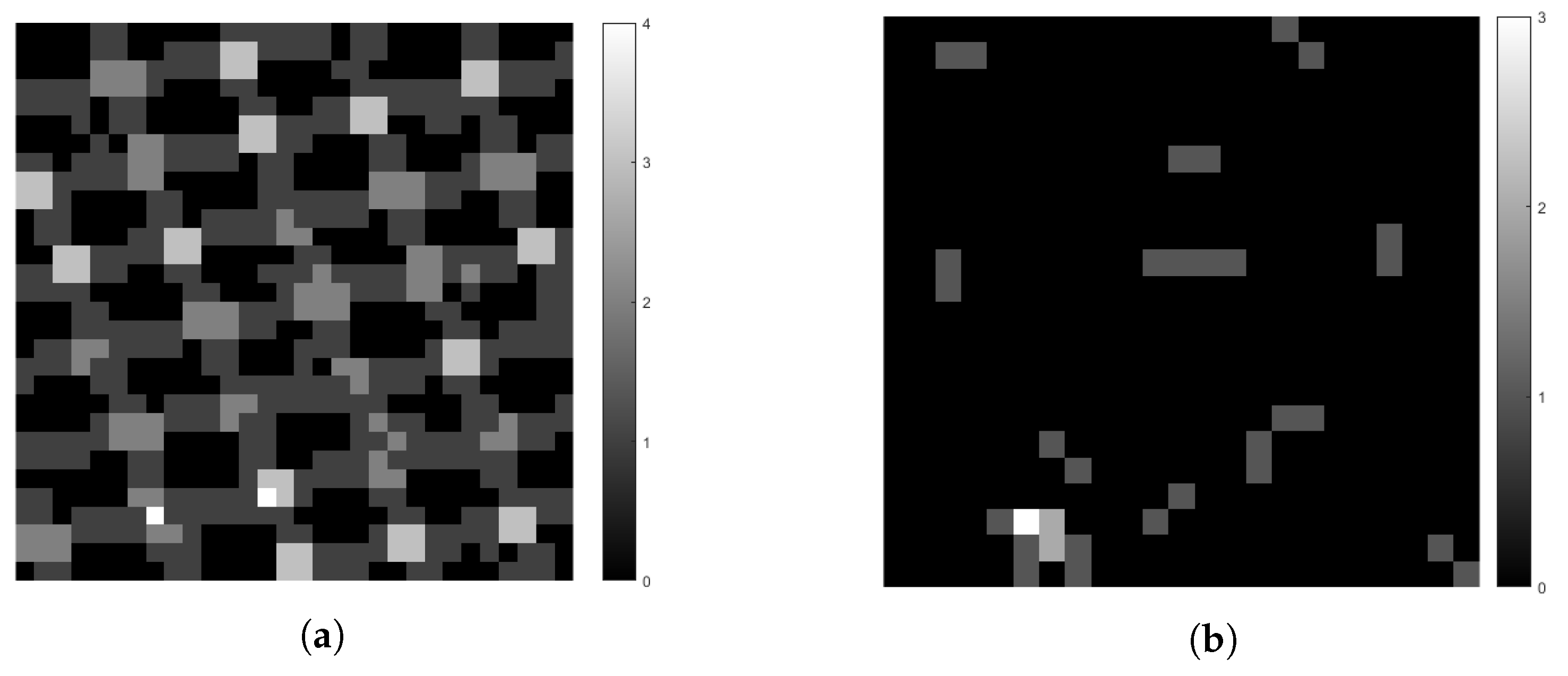
Figure 3.
(a) RGB imagery of SJERHS; (b) Validated abundance map reference data (AMRD) at the 10 m × 10 m aggregation scale for SJERHS, with ground cover classes (left-to-right and top-to-bottom): PV, NPV, BS, Rock, and Other (Roof).
Figure 3.
(a) RGB imagery of SJERHS; (b) Validated abundance map reference data (AMRD) at the 10 m × 10 m aggregation scale for SJERHS, with ground cover classes (left-to-right and top-to-bottom): PV, NPV, BS, Rock, and Other (Roof).
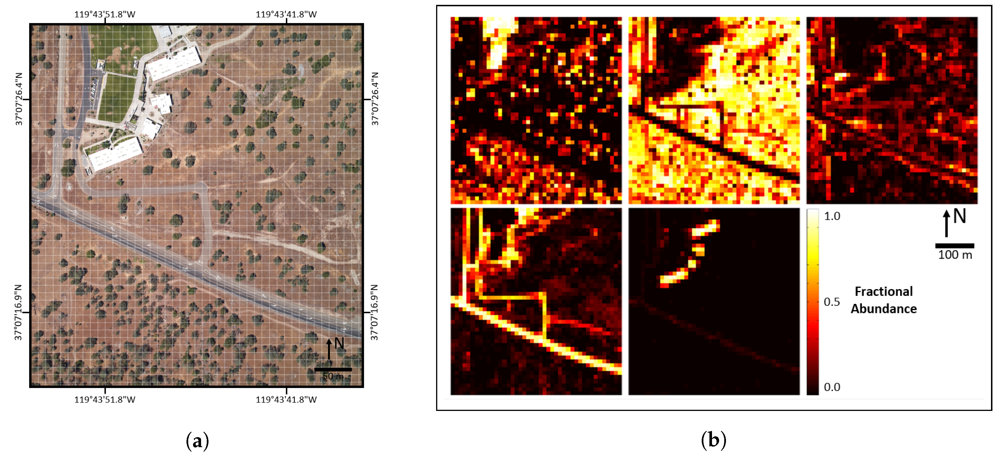
Figure 4.
(a) RGB imagery of SJER116; (b) Validated abundance map reference data (AMRD) at the 10 m × 10 m aggregation scale for SJER116, with ground cover classes (left-to-right and top-to-bottom): PV, NPV, BS, Rock, and Other.
Figure 4.
(a) RGB imagery of SJER116; (b) Validated abundance map reference data (AMRD) at the 10 m × 10 m aggregation scale for SJER116, with ground cover classes (left-to-right and top-to-bottom): PV, NPV, BS, Rock, and Other.

Figure 5.
(a) RGB imagery of SOAP299; (b) Validated abundance map reference data (AMRD) at the 10 m × 10 m aggregation scale for SOAP299, with ground cover classes (left-to-right and top-to-bottom): PV, NPV, BS, Rock, and Other.
Figure 5.
(a) RGB imagery of SOAP299; (b) Validated abundance map reference data (AMRD) at the 10 m × 10 m aggregation scale for SOAP299, with ground cover classes (left-to-right and top-to-bottom): PV, NPV, BS, Rock, and Other.

Figure 6.
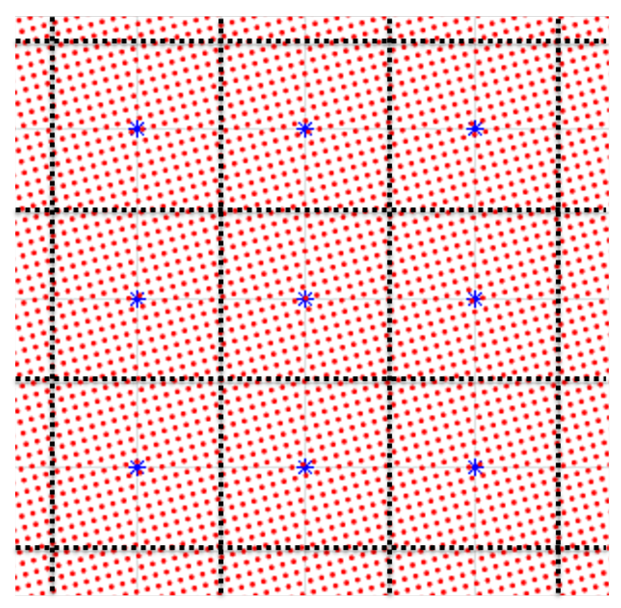
This figure is a visualization of a single rotation, scale, and translation iteration within the SWSC algorithm. Blue stars represent coarse pixels centers, red dots represent fine pixel centers, and black lines represent the nominal divisions between coarse sensors for rectangular aggregation.
Figure 6.
This figure is a visualization of a single rotation, scale, and translation iteration within the SWSC algorithm. Blue stars represent coarse pixels centers, red dots represent fine pixel centers, and black lines represent the nominal divisions between coarse sensors for rectangular aggregation.

Figure 7.
Mean values in these figures were generated by sweeping across possible (a) rotation; (b) scale; and (c) translation values. The minimum mean locations for rotation, scale, and translation were selected as the optimal parameters for spatial alignment between NEON SI and AVIRIS Unorthorectified data for the SJERHS scene.
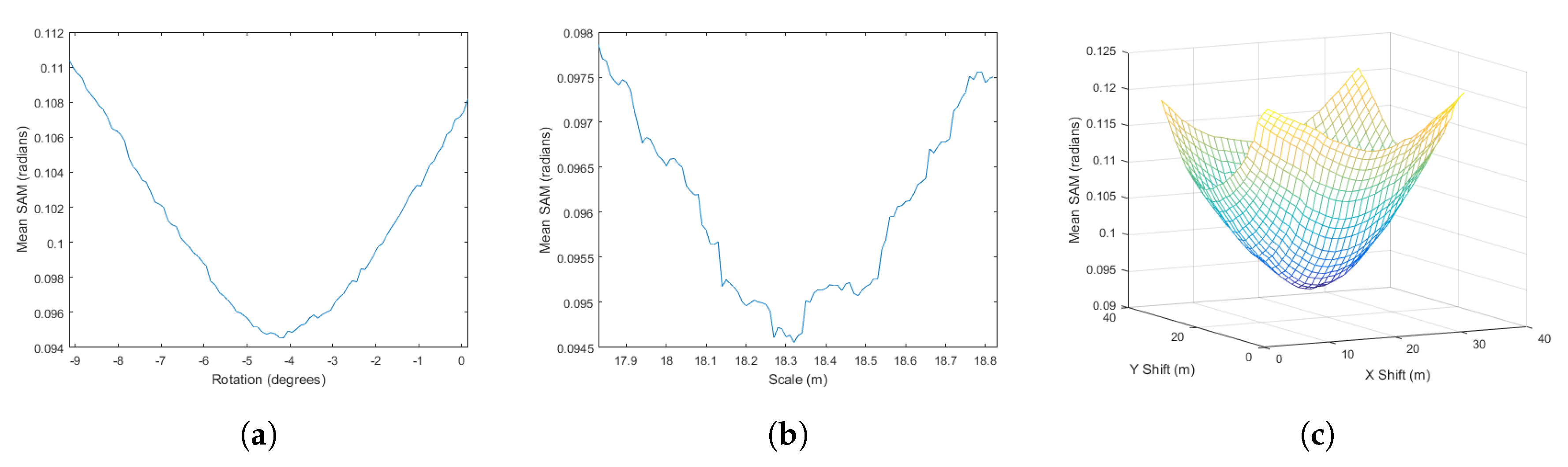
Figure 8.
Mean values in these figures were generated by sweeping across possible translation values. The mean minimums represent the optimal translation for spatial alignment between NEON SI and (a) AVIRIS Orthorectified; (b) AVIRIS Unorthorectified; (c) NEON 15 m; (d) NEON 29 m, for the SJERHS scene.

Figure 9.
FCLS unmixing abundances versus rectangular aggregated AMRD for all three scenes of AVIRIS Unorthorectified data combined, including regression line and , for (a) PV; (b) NPV; (c) BS; and (d) Rock.
Figure 9.
FCLS unmixing abundances versus rectangular aggregated AMRD for all three scenes of AVIRIS Unorthorectified data combined, including regression line and , for (a) PV; (b) NPV; (c) BS; and (d) Rock.
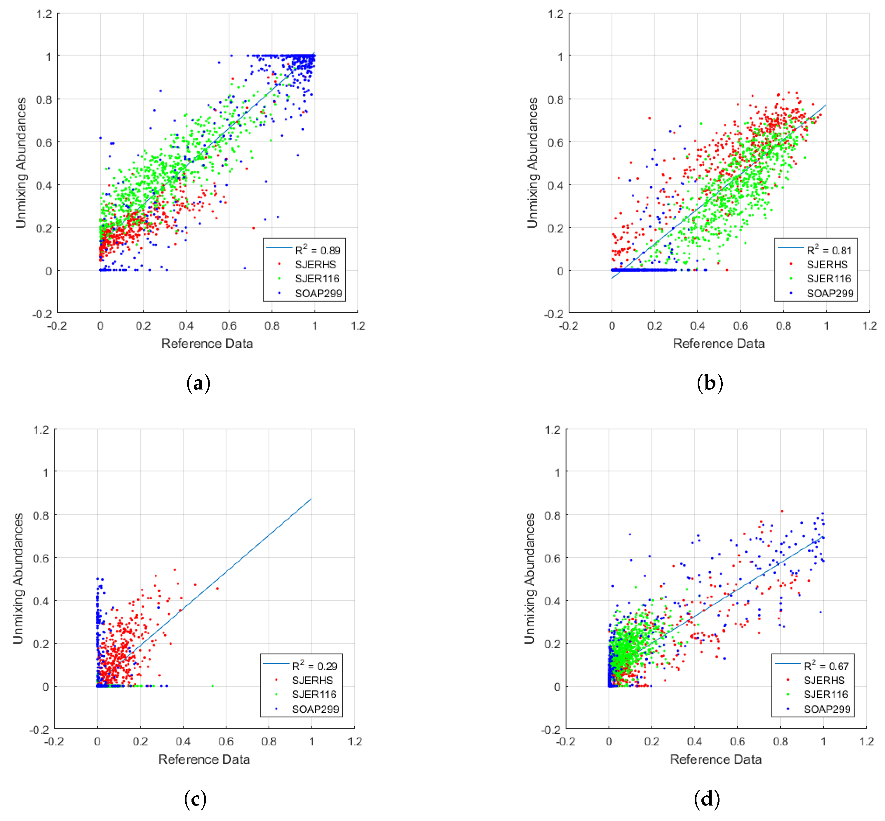
Figure 10.
Unmixing abundances versus rectangular aggregated AMRD for data from all four classes and all three scenes combined, including the regression line and , for (a) AVIRIS Unortho/LS unmixing, (b) NEON 15 m/LS unmixing, (c) AVIRIS Unortho/NNLS unmixing, (d) NEON 15 m/NNLS unmixing, (e) AVIRIS Unortho/FCLS unmixing, and (f) NEON 15 m/FCLS unmixing.


Table 1.
National Ecological Observatory Network (NEON)/Airborne Visible/Infrared Imaging Spectrometer(AVIRIS) Data Details.
Table 1.
National Ecological Observatory Network (NEON)/Airborne Visible/Infrared Imaging Spectrometer(AVIRIS) Data Details.
| Data | GSD | Altitude | Spectra | Bands | Processing | Date/Time (PDT) |
|---|---|---|---|---|---|---|
| NEON RGB | 0.25 m | 1 km | 0.4–0.7 μm | 3 | N/A | 13 June 2013/1430 |
| NEON IS | 1 m | 1 km | 0.4–2.5 μm | 428 | AtmCal/OrthRect | 13 June 2013/1430 |
| AVIRIS IS Ortho | 15 m | 20 km | 0.4–2.5 μm | 224 | AtmCal/OrthRect | 13 June 2013/1058 |
| AVIRIS IS Unortho | 18 m | 20 km | 0.4–2.5 μm | 224 | AtmCal | 13 June 2013/1058 |
| NEON 15 m | 15 m | 1 km | 0.4–2.5 μm | 428 | Conv/DownSamp | 13 June 2013/1430 |
| NEON 29 m | 29 m | 1 km | 0.4–2.5 μm | 428 | Conv/DownSamp | 13 June 2013/1430 |
Table 2.
Accuracy assessment of RSRD-NNLS across 51 validation plots from all three study scenes. Data are expressed in terms of percent coverage area difference from MOA [8].
Table 2.
Accuracy assessment of RSRD-NNLS across 51 validation plots from all three study scenes. Data are expressed in terms of percent coverage area difference from MOA [8].
| Class (c) | ||||
|---|---|---|---|---|
| PV | 1.6 | 3.8 | −0.1 | 3.8 |
| NPV | −1.5 | 7.2 | −4.4 | 1.1 |
| BS | −4.5 | 6.4 | −7.0 | −3.7 |
| Rock | 4.3 | 8.0 | 3.0 | 7.2 |
Table 3.
The values in this table represent minimum mean values (radians) at the location of optimal alignment between NEON SI and coarse scale imagery for the SJERHS, SJER116, and SOAP299 scenes. Values are listed for the PSF and rectangular aggregation methods.
Table 3.
The values in this table represent minimum mean values (radians) at the location of optimal alignment between NEON SI and coarse scale imagery for the SJERHS, SJER116, and SOAP299 scenes. Values are listed for the PSF and rectangular aggregation methods.
| Coarse Scale Imagery | SJERHS | SJER116 | SOAP299 | |||
|---|---|---|---|---|---|---|
| PSF | Rect | PSF | Rect | PSF | Rect | |
| AVIRIS Ortho | 0.0697 | 0.0775 | 0.0754 | 0.0854 | 0.1367 | 0.1405 |
| AVIRIS Unortho | 0.0946 | 0.0980 | 0.0963 | 0.0975 | 0.1209 | 0.1256 |
| NEON 15 m | 0.0041 | 0.0163 | 0.0060 | 0.0177 | 0.0053 | 0.0167 |
| NEON 29 m | 0.0046 | 0.0163 | 0.0024 | 0.0125 | 0.0030 | 0.0192 |
Table 4.
Comparison of mean absolute error (%) between reference data and unmixing abundances by image type, unmixing type, and reference data type.
Table 4.
Comparison of mean absolute error (%) between reference data and unmixing abundances by image type, unmixing type, and reference data type.
| Image Type | ||||
|---|---|---|---|---|
| AVIRIS Ortho | 18.88 | 19.11 | 19.48 | 19.14 |
| AVIRIS Unortho | 26.80 | 28.11 | 28.62 | 28.22 |
| NEON 15 m | 5.87 | 6.92 | 7.56 | 7.31 |
| NEON 29 m | 5.41 | 6.41 | 3.28 | 7.51 |
| Unmix Type | ||||
| LS | 28.02 | 28.25 | 28.60 | 28.35 |
| NNLS | 8.41 | 9.57 | 10.41 | 9.60 |
| FCLS | 6.29 | 7.60 | 8.04 | 8.14 |
| Reference Type | ||||
| Rect | 14.48 | 15.40 | 15.92 | 15.62 |
| PSF | 14.00 | 14.88 | 15.44 | 15.10 |
Table 5.
Comparison of mean absolute error (%) between reference data and unmixing abundances by image type and reference data type, when LS unmixing results were excluded from analysis.
Table 5.
Comparison of mean absolute error (%) between reference data and unmixing abundances by image type and reference data type, when LS unmixing results were excluded from analysis.
| Image Type | ||||
|---|---|---|---|---|
| AVIRIS Ortho | 10.87 | 11.49 | 12.04 | 11.54 |
| AVIRIS Unortho | 10.38 | 12.26 | 13.00 | 12.35 |
| NEON 15 m | 4.07 | 5.35 | 5.99 | 5.87 |
| NEON 29 m | 4.06 | 5.23 | 5.88 | 5.71 |
| Reference Type | ||||
| Rect | 7.59 | 8.86 | 9.48 | 9.14 |
| PSF | 7.10 | 8.31 | 8.98 | 8.60 |
Table 6.
Comparison of mean absolute error (%) between reference data and unmixing abundances by unmixing type and reference data type, when AVIRIS imagery results were excluded from analysis.
Table 6.
Comparison of mean absolute error (%) between reference data and unmixing abundances by unmixing type and reference data type, when AVIRIS imagery results were excluded from analysis.
| UnmixType | ||||
|---|---|---|---|---|
| LS | 8.77 | 9.42 | 10.09 | 9.54 |
| NNLS | 5.01 | 6.17 | 7.01 | 6.40 |
| FCLS | 3.13 | 4.42 | 4.87 | 5.19 |
| Reference Type | ||||
| Rect | 5.84 | 6.90 | 7.52 | 7.27 |
| PSF | 5.44 | 6.43 | 7.13 | 6.82 |
Table 7.
Specific mean absolute error (%) results for the combination of AVIRIS Unorthorectified imagery, FCLS unmixing, and rectangular aggregation of AMRD.
Table 7.
Specific mean absolute error (%) results for the combination of AVIRIS Unorthorectified imagery, FCLS unmixing, and rectangular aggregation of AMRD.
| PV (c = 1) | NPV (c = 2) | BS (c = 3) | Rock (c = 4) | ||
|---|---|---|---|---|---|
| MAEc | 11.17 | 13.69 | 4.25 | 8.31 | 9.35 |
| MA-MAEc | 10.25 | 14.87 | 7.12 | 11.07 | 10.83 |
| CIA-MAEc,ll | 11.11 | 17.26 | 8.92 | 10.14 | 11.86 |
| CIA-MAEc,ul | 13.85 | 12.87 | 6.57 | 13.25 | 11.63 |
Table 8.
Regression Table.
| PV | NPV | BS | Rock | All | |
|---|---|---|---|---|---|
| AVIRIS Unortho/LS | |||||
| Slope | 0.67 | 2.41 | 3.06 | −0.04 | 1.49 |
| Intercept | 0.13 | −0.58 | −0.36 | −0.55 | −0.37 |
| 0.57 | 0.57 | 0.07 | 0.00 | 0.16 | |
| AVIRIS Unortho/NNLS | |||||
| Slope | 0.36 | 0.72 | 0.66 | 0.42 | 0.55 |
| Intercept | 0.18 | −0.04 | 0.01 | 0.07 | 0.05 |
| 0.45 | 0.81 | 0.32 | 0.55 | 0.68 | |
| AVIRIS Unortho/FCLS | |||||
| Slope | 0.89 | 0.81 | 0.86 | 0.62 | 0.85 |
| Intercept | 0.13 | −0.04 | 0.02 | 0.07 | 0.04 |
| 0.89 | 0.80 | 0.29 | 0.67 | 0.81 | |
| NEON 15 m/LS | |||||
| Slope | 0.70 | 1.00 | 1.14 | 1.00 | 0.88 |
| Intercept | 0.05 | −0.02 | −0.01 | −0.02 | 0.00 |
| 0.85 | 0.78 | 0.24 | 0.76 | 0.79 | |
| NEON 15 m/NNLS | |||||
| Slope | 0.66 | 1.06 | 0.88 | 0.95 | 0.86 |
| Intercept | 0.04 | −0.02 | −0.00 | −0.01 | 0.01 |
| 0.84 | 0.95 | 0.79 | 0.95 | 0.90 | |
| NEON 15 m/FCLS | |||||
| Slope | 1.01 | 1.06 | 0.98 | 0.99 | 1.03 |
| Intercept | −0.02 | −0.00 | −0.00 | −0.00 | −0.01 |
| 0.98 | 0.97 | 0.80 | 0.97 | 0.98 |
© 2017 by the authors. Licensee MDPI, Basel, Switzerland. This article is an open access article distributed under the terms and conditions of the Creative Commons Attribution (CC BY) license (http://creativecommons.org/licenses/by/4.0/).
Share and Cite
MDPI and ACS Style
Williams, M.D.; Kerekes, J.P.; Aardt, J.V. Application of Abundance Map Reference Data for Spectral Unmixing. Remote Sens. 2017, 9, 793. https://doi.org/10.3390/rs9080793
AMA Style
Williams MD, Kerekes JP, Aardt JV. Application of Abundance Map Reference Data for Spectral Unmixing. Remote Sensing. 2017; 9(8):793. https://doi.org/10.3390/rs9080793
Chicago/Turabian StyleWilliams, McKay D., John P. Kerekes, and Jan Van Aardt. 2017. "Application of Abundance Map Reference Data for Spectral Unmixing" Remote Sensing 9, no. 8: 793. https://doi.org/10.3390/rs9080793
Note that from the first issue of 2016, this journal uses article numbers instead of page numbers. See further details here.