
Effect of Label Noise on the Machine-Learned Classification of Earthquake Damage


1
Department of Computer Science, Cornell University, 402 Gates Hall, Ithaca, NY 14850, USA
2
Jet Propulsion Laboratory, California Institute of Technology, 4800 Oak Grove Drive, Pasadena, CA 91109, USA
3
Michigan Technological University, 1400 Townsend Drive, Houghton, MI 49931, USA
*
Author to whom correspondence should be addressed.
Remote Sens. 2017, 9(8), 803; https://doi.org/10.3390/rs9080803
Submission received: 30 May 2017
/
Revised: 17 July 2017
/
Accepted: 28 July 2017
/
Published: 4 August 2017
(This article belongs to the Special Issue Earth Observation to Support Disaster Preparedness and Disaster Risk Management)
Abstract
:Automated classification of earthquake damage in remotely-sensed imagery using machine learning techniques depends on training data, or data examples that are labeled correctly by a human expert as containing damage or not. Mislabeled training data are a major source of classifier error due to the use of imprecise digital labeling tools and crowdsourced volunteers who are not adequately trained on or invested in the task. The spatial nature of remote sensing classification leads to the consistent mislabeling of classes that occur in close proximity to rubble, which is a major byproduct of earthquake damage in urban areas. In this study, we look at how mislabeled training data, or label noise, impact the quality of rubble classifiers operating on high-resolution remotely-sensed images. We first study how label noise dependent on geospatial proximity, or geospatial label noise, compares to standard random noise. Our study shows that classifiers that are robust to random noise are more susceptible to geospatial label noise. We then compare the effects of label noise on both pixel- and object-based remote sensing classification paradigms. While object-based classifiers are known to outperform their pixel-based counterparts, this study demonstrates that they are more susceptible to geospatial label noise. We also introduce a new labeling tool to enhance precision and image coverage. This work has important implications for the Sendai framework as autonomous damage classification will ensure rapid disaster assessment and contribute to the minimization of disaster risk.
1. Introduction
Two major innovations have improved our ability to rapidly assess damage in the aftermath of a major earthquake event: high spatial resolution remote sensing imagery and online crowdsourcing [1,2]. In the two days after the 2011 earthquake in New Zealand, nearly 70,000 unique online visitors amassed 779 reports that informed the activities of local volunteers who helped clear more than 360,000 tons of silt and rubble [3]. This effort effectively allocated assistance to the neediest areas and enabled accurate estimation of the cost of recovery. Due to the success of crowdsourcing efforts, damage assessment has largely shifted to websites such as Tomnod and OpenStreetMap (OSM) [4].
Despite success stories associated with crowdsourced damage assessment, the quality of amateur data is a major concern. A study of the 2010 crowdsourced effort that mapped damage in high-resolution images of the Haiti earthquake validated crowd annotations against ground observations and Pictometry data. This study found the accuracy of the crowdsourced effort to range between 20% and 80% depending on the damage class and data source used for validation [5]. One Red Cross member reported after the 2015 Nepal earthquake that “more than half of the contributors are completely new to OSM and are making their very first edits...Whilst that’s undoubtedly a good thing, many are making mistakes and need to be trained along the way” [6]. Many projects have tried to address data quality issues by requiring volunteer training or a minimum level of expertise. However, projects seeking to improve data quality experience trade-offs in terms of increased costs to implement quality controls and decreased volunteer participation [7]. Meanwhile, the number of remotely-sensed data products with increased spatial, spectral and temporal coverage is proliferating. It is unclear that crowdsourcing can continue to be the primary method for the annotation of damage in the era of big data. If crowdsourced volunteers can be shifted toward the generation of training data, then automated classifiers can classify damage in large amounts of imagery in a fraction of the time.
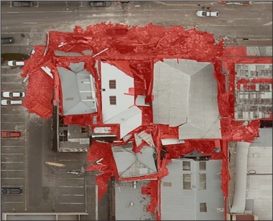
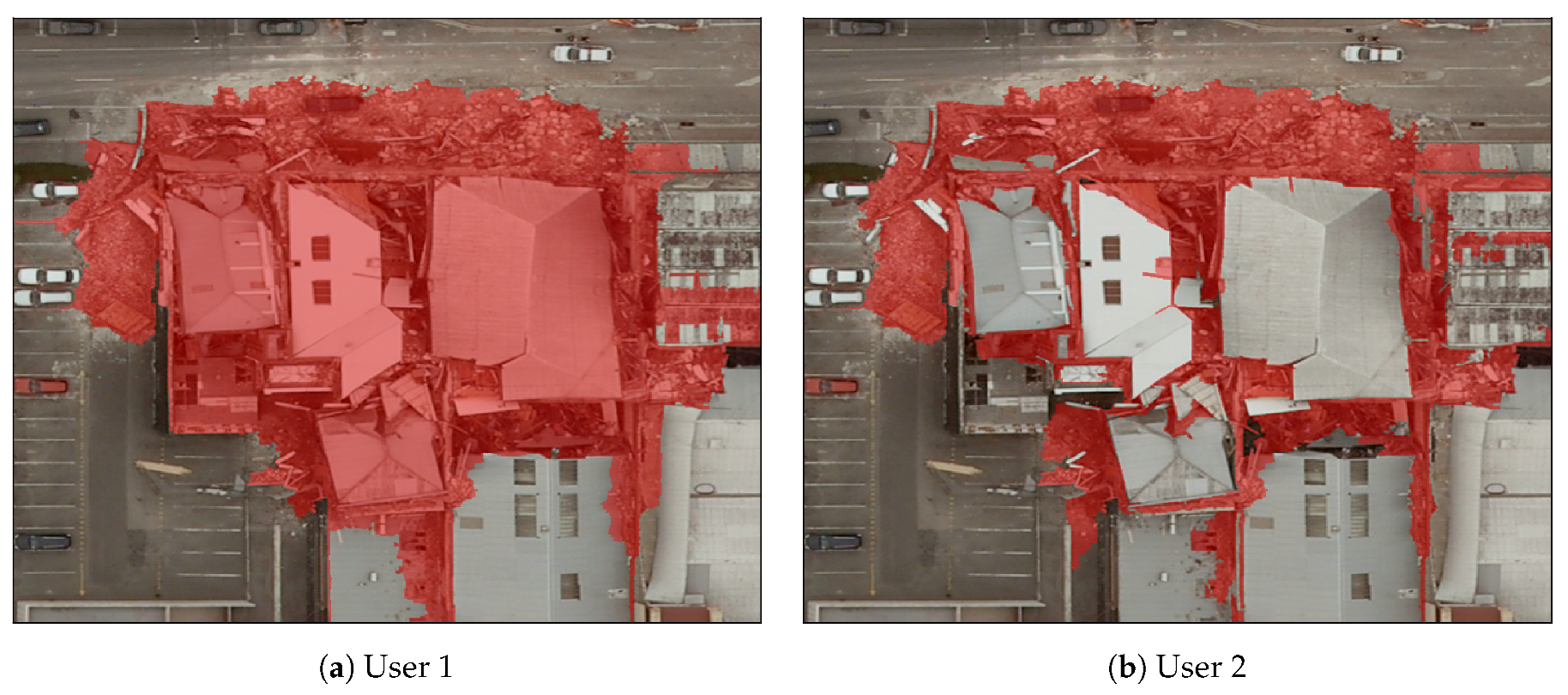
This study focuses on the machine-learned classification of rubble in remotely-sensed images taken in the aftermath of an earthquake event. Automated classifiers have shown promise detecting rubble in remote sensing images [8]. However, the impact of training data quality on classifier performance has received little attention in both earthquake damage detection and remote sensing as a whole. Even within the machine learning literature, label noise is usually simulated and assumed to be distributed uniformly [9,10]. In reality, objects that occur near rubble, like buildings and streets, are more likely to be mislabeled than unrelated structures, such as water or trees. Similar problems may arise if labeling instructions are not carefully specified. Figure 1 is an example of two user annotations of the same damaged structure where different labeling tools and instructions were used. User 1 was tasked with labeling “damage” and marked intact roofs that belonged to damaged buildings, an ambiguity that would confuse a classifier whose annotations of damage largely consist of rubble. We call this type of label confusion that occurs in spatially-contiguous regions of remote sensing imagery geospatial label noise. The effects of geospatial label noise can be seen in the map in Figure 2. This figure shows five individuals’ attempts to identify earthquake damage in an image. Bright red regions indicate areas that all labelers believed contained damage. Dark red regions indicate areas that only one labeler did. Noticeably, regions in which labelers tend to disagree with the majority vote happen in close geospatial proximity to regions in which all labelers agree.
In this paper, we compare how geospatial label noise affects classifiers from the two major remote sensing classification paradigms: pixel-based and object-based. Object-based methods are also known as Geographic Object-Based Image Analysis (GEOBIA) [11] and assume a pre-processing step of image segmentation that partitions the scene into relatively homogeneous segments that ideally correspond to semantically-meaningful objects (e.g., cars, buildings, roads). Then, a feature extraction process runs upon each object to yield measurements that characterize the object’s shape, texture and colors. Pixel-based classification uses only the spectral content of each pixel or passes a sliding window over each pixel to capture contextual textural and spectral features.
We conduct experiments with both pixel- and object-based classifiers on two large orthorectified images of downtown Christchurch, New Zealand, taken after the 22 February 2011 earthquake. Our results confirm the results from the GEOBIA literature that object-based classifiers outperform pixel-based classifiers when trained on data that are free of label noise. However, the performance of object-based classifiers degrades more quickly and sinks below the performance of pixel-based classifiers as training data are mislabeled with increasing amounts of geospatial label noise. We experiment with two types of simulated geospatial label noise and demonstrate the use of a new labeling tool that is less prone to introducing noise during the labeling process.
The remainder of the paper includes the following sections. Section 2 describes related work on remote sensing classification, random forest classifiers and label noise. Section 3 introduces the data and imagery used in the experiments. Section 4 describes the experimental setup. Section 5 presents the results from all noise experiments. Section 6 summarizes our findings and presents their implications for disaster preparedness and risk management.
2. Related Work
2.1. Pixel- vs. Object-Based Classifiers
Pixel-based classifiers were popular in the later 20th Century [12] and are still used for lower resolution classification tasks at scales where shapes are largely uninformative, such as in rainforest classification [13,14]. However, at higher resolutions, pixel-based approaches face limitations. Increased spatial resolution creates settings in which scene objects are significantly larger than the sensor’s resolution cell. These settings, called H-resolution situations, expand the number and variety of pixels in small structures such as buildings and trees [15]. This increased intra-class variance of pixels diminishes the predictive capabilities of pixel-based approaches, an issue referred to as the H-resolution problem [11]. However, this improved detail enables the use of image segmentation in order to partition the scene into objects that ideally correspond to natural features in the scenes. Object construction allows for the calculation of features that encapsulate new information about an object’s context and shape, in addition to texture and color. In high resolution imagery, the combination of textural, shape and color features allows GEOBIA classifiers to outperform pixel-based methods.
2.2. Label Noise
Label noise is broadly categorized into three models: Noise Completely at Random (NCAR), Noise at Random (NAR), or Noise Not at Random (NNAR) [16]. NCAR occurs in binary classification when every label is equally probable of being wrong and may be modeled by a simple Bernoulli random variable, independent of class. NAR occurs in binary classification when one class is more likely to be modeled incorrectly than the other and may be modeled by a Bernoulli random variable with different prior probabilities for each class. These first two types of noise have been greatly analyzed mathematically and their simple probability functions make them easy to simulate. Classifier performance is often only evaluated against these two models of noise [9,10].
NNAR is the most elusive noise model in the machine learning literature [16]. NNAR is modeled by a probability function dependent on the feature space of the data rather than its labeling scheme. In one of the few studies that attempts to simulate NNAR noise, it is modeled with a probability density function that is dependent on the distance of an example from the classification boundary [17]. Another study of label noise in a multi-class setting simulated label noise by swapping labels between similar classes. Like the experiments in [17], these studies analyze NNAR based on class ambiguity and proximity in the feature space as opposed to geospatial proximity [18]. Although these methods model noise caused by class ambiguity, they do not model geospatial label noise that occurs in remote sensing classification.
In the remote sensing literature, several papers have discussed both correlated and uncorrelated imperfect ground reference data [19,20]. These methods of label noise analysis study alterations to the confusion matrix of classifier predictions against ground observations and compromises counts of false positives, true positives, false negatives and true negatives. The alteration of a confusion matrix to generate prior probabilities simulates NAR label noise, but not NNAR.
Geospatial label noise as we define it falls under the NNAR category. Label noise for rubble is likely to be restricted to sidewalks and rooftops because they are in closer geospatial proximity to the rubble target class. This type of label noise cannot be modeled using distance from the classification boundary because, although rubble and rooftops are in close geospatial proximity, the smooth textures and simple geometries of roads and rooftops are dissimilar to the heterogeneous textures and jagged boundaries of rubble. The likely source of error is not the labeler’s inability to distinguish between an intact road versus rubble, but imprecision in labeling due to geospatial proximity and the use of certain digital labeling tools.
3. Study Area and Data
Study Site
Figure 3 shows the location studied in this paper. The images were taken following the 22 February 2011 earthquake. The study site is an urban area in downtown Christchurch, New Zealand, between the latitudes of and and the longitudes of and . The area contains residential housing, a green park and a construction quarry that is always confused with rubble. The entire region is filled with grid-like streets and large commercial buildings.
The images were released on 24 February 2011, by New Zealand Aerial Mapping two days after a magnitude 6.3 earthquake was recorded [21]. The images were taken with a UCXp sensor at 0.1-m spatial resolution and are comprised of red, green and blue spectral bands. The images were stitched together and orthorectified by re-projecting from the center of each image to minimize building lean. Our study is based on Tiles 1-0003-0002 and 1-0003-0003, each of which is pixels in size.
4. Experiments
We conduct two major groups of experiments. In the first, we simulate label noise in order to measure the impact of different types and amounts of label noise on both pixel- and object-based classification. In the second, we solicited three human-labeled training sets that were labeled with different labeling methodologies and tools in order to measure how different labeling methods impact classification results.
4.1. Experimental Setup
In this section, we describe our experimental platform and its software implementation. We first describe the overall classification framework, followed by the feature sets extracted for object- and pixel-based classification, the methods of simulating both random, and geospatial label noise and our performance metrics.
4.1.1. Classification
Our classifier of choice is the random forest [22], a popular classifier known for its resilience to overfitting and label noise [9,10,16]. We use scikit-learn’s implementation of the random forest for classification, setting the number of trees at 85 and all other parameters at default values. In order to quantify the uncertainty of the random forest decision, the share of trees that voted for rubble is used as a posterior probability. By converting the output into a probability, we can evaluation our results at arbitrary decision thresholds between 0.0 and 1.0 and generate Receiver Operator Characteristic (ROC) curves, described in more detail in Section 4.1.4.
We perform two versions of each experiment where Tiles 0002 and 0003 are used for training and testing, and vice versa. For each direction, we present the mean and standard deviation of ten experimental iterations since the random forest has non-deterministic behavior.
4.1.2. Feature Extraction
In pixel-based classification, the unit of classification is the individual pixel. With object-based classification, the unit of classification is a segment produced via segmentation of the image. Pixel-based features include the spectral content of the individual pixel along with features extracted from an neighborhood of pixels centered on the pixel in question. For object-based classification, we extract object-based features from the segments produced via image segmentation.
We used eCognition’s built-in implementation of the Baatz Schäpe algorithm [23] for image segmentation. An important parameter, called the scale parameter, sets the average size of the segment. When the scale parameter is set to 1000, multiple city blocks are included in one segment. At smaller scales, such as 50, rubble patches are divided into dozens of segments. We additionally set shape and compactness parameters to and leave all other parameters set to eCognition’s default settings.Classification is performed on a single segmentation, but features from other segmentations with larger scale parameter values provide encompassing segments that contextualize features and improve classification in a hierarchical approach. For our experiments, we classify at scale 50 and generate contextual features from scale 100.
For both the object- and pixel-based classifiers, we generate features that reflect the random, textured qualities of rubble. The features we calculate for the pixel-based classifier are edge densities, Histograms of Oriented Gradients [24] and average color. The edge density is computed by applying a canny edge detector (with thresholds 50 and 100) to the image and then subjecting the neighborhood around the pixel to a normalized box filter. We implemented the edge density feature using the functions and from the python implementation of the openCV computer vision library [25]. We implement the Histogram of Oriented Gradients (HOG) by using the filter to calculate partial derivatives of the image in the x and y directions, converting both gradient images to polar coordinates using and creating a 16-bin histogram for each pixel using a sliding window of the polar coordinate image. We then used scikit-image’s function [26]. We calculated average color by taking a Gaussian blur (using ) over each band using a sliding window size of . The total number of pixel features is 23, comprised of 3 RGB pixel values, 3 average RGB pixel values, 16 HOG bins and 1 measure of edge density.
For the GEOBIA classifier, we use these same features calculated on individual segments rather than window cells, as well as additional features collected using eCognition detailed in Table 1. These features measure the texture, color and shape of each object. Figure 4 shows the top 24 features in terms of their importance to the random forest classifier.
4.1.3. Label Noise Simulation
Our experiments using label noise simulation focus on the problem of “over-labeling” rubble. This means that we assume users tend to draw generous boundaries around rubble and falsely label non-rubble as rubble, rather than mistaking rubble as something non-rubble or some type of object that is not damage. Our simulations flip segments from a finely segmented image (using scale parameter 50) rather than individual pixels, so that we can use the same simulated noise for both object- and pixel-based classifiers.
We simulate random noise and two varieties of geospatial label noise. We present the performance of the classifier as a function of the percentage of the rubble class that is mislabeled, where the x-axes will be labeled percent noise. For the object classifier, this value is the percentage of segments, whereas in the pixel classifier, it is the percentage of pixels. Starting with a noise-free labeling, we iteratively select new non-rubble training segments to mislabel as rubble in batches of 100. Depending on the experiment, these 100 segments are selected in the following ways:
- NAR: NAR or random noise is simulated such that our labeled rubble class is flipped with probability zero while non-rubble is flipped with probability , where is the number of non-rubble segments in an image. At the start of the experiment, 19,024 of the 19,745 segments are non-rubble, so the probability that a non-rubble segment is flipped is .
- Building noise: This type of NNAR represents the scenario in which a labeler misinterprets the task and includes parts of the buildings adjacent to the rubble. For this class-specific contamination, rather than flipping all non-rubble labels with equal likelihood, we flip only the labels of non-rubble segments containing buildings.
- Geospatial noise: This type of noise is simulated by applying a morphological dilation to the areas correctly labeled as rubble. Non-rubble data that are geospatially closer to rubble are therefore more likely to be corrupted. This emulates imprecise labeling tools because the regions of interest have not changed, only the width of the label. An example of this process’s appearance can be seen in Figure 5.
4.1.4. Performance Evaluation and Metrics
The default performance metric in machine learning is accuracy. However, for classification problems like rubble detection where of the data are in the non-rubble class, a classifier that predicts all data as non-rubble will result in a accuracy, which is a misleading result. We use the False Positive Rate (FPR) and the True Positive Rate (TPR) defined as follows:
Definition 1.
Definition 2.
By default, the decision threshold that determines whether an example is positive or negative is 0.5. However, in order to consider the full range of possible decision thresholds in the evaluation of our classifier performance, we use Receiver Operator Characteristic (ROC) curves, which form a continuum over all possible decision thresholds. ROC curves can be summarized as a single value, called Area Under the Curve (AUC). A large AUC, close to one, indicates a high-performing classifier, whereas an AUC of 0.5 indicates random classification.
In order to ensure comparability between pixel- and object-based classifiers, we weight the classification of each object in the object-based classification by the number of pixels it contains.
4.2. Human-Labeled Training Data and Labeling Tools
We solicited three human-labeled training sets for our final experiment, each of which made use of a different labeling tool. Table 2 describes for each training dataset the labeling tool and methodology used.
Dataset uses QGIS’s polygon drawing tool. This interface works by allowing the user to draw arbitrary polygons by specifying vertices with a mouse. An example of labeling rubble using this tool can be seen in Figure 6a. We found that this method of labeling had a number of problems. First, labeling with polygons is imprecise for identifying rubble. Polygon tools are helpful for when a class object can be easily outlined with a simple shape (e.g., buildings). Rubble is inherently random and often concave in shape. It takes dozens of points to carefully outline one small patch. Second, it is difficult to ensure that the entire image has been labeled. Many images are extremely large and require zooming in 10 to 20 times to label in detail. When zooming and panning around large images, it is easy to miss unlabeled sections of the map entirely. Dataset was also labeled with an objective of identifying damage as opposed to rubble. This caused the labeler to annotate non-rubble pixels as damage. Figure 7d reveals that the labeler annotated the relatively intact roof of a damaged building as damage. This tendency towards over-labeling rubble resulted in large amounts of geospatial label noise.
Dataset was solicited in response to the noise issues with Dataset . was labeled with the objective of conservatively identifying areas that were rubble. This labeler used eCognition’s segmentation (at scale parameter 25) and selected only those segments that he/she was certain contained rubble. As a result, large sections of each image were not labeled, and many rubble areas were omitted from the training set.
To solve both of these issues, we developed a web-based labeling tool that labels objects created via image segmentation. First, each image is divided into a number of tiles that may be zoomed into for reference. Each tile is outlined in green when seen, giving the user an indicator of whether they have omitted a section of the map. Figure 6c shows an example of this view after labeling the entire map. When the user zooms into a tile, the map is further partitioned, in this case by a scale 50 segmentation. Each segment is outlined when hovered over. To label areas as rubble, users click and drag across relevant regions, causing the segments covering those regions to glow red. Because the segmentation is small and adheres to the natural edges of the image, painting these segments is both precise and fast. An example of this editing view can be seen in Figure 6b. All segments highlighted in red have been painted by the user as rubble. In the figure, the user’s mouse hovers over the car in the center, and the relevant segment is outlined in white. Although it is possible to label in this way with both eCognition and QGIS by adjusting multiple settings, both are full-featured GIS applications that may be unfriendly for inexperienced users performing a one-off task. Our tool is lightweight and easily deployed on a web server. Dataset was labeled with this tool.
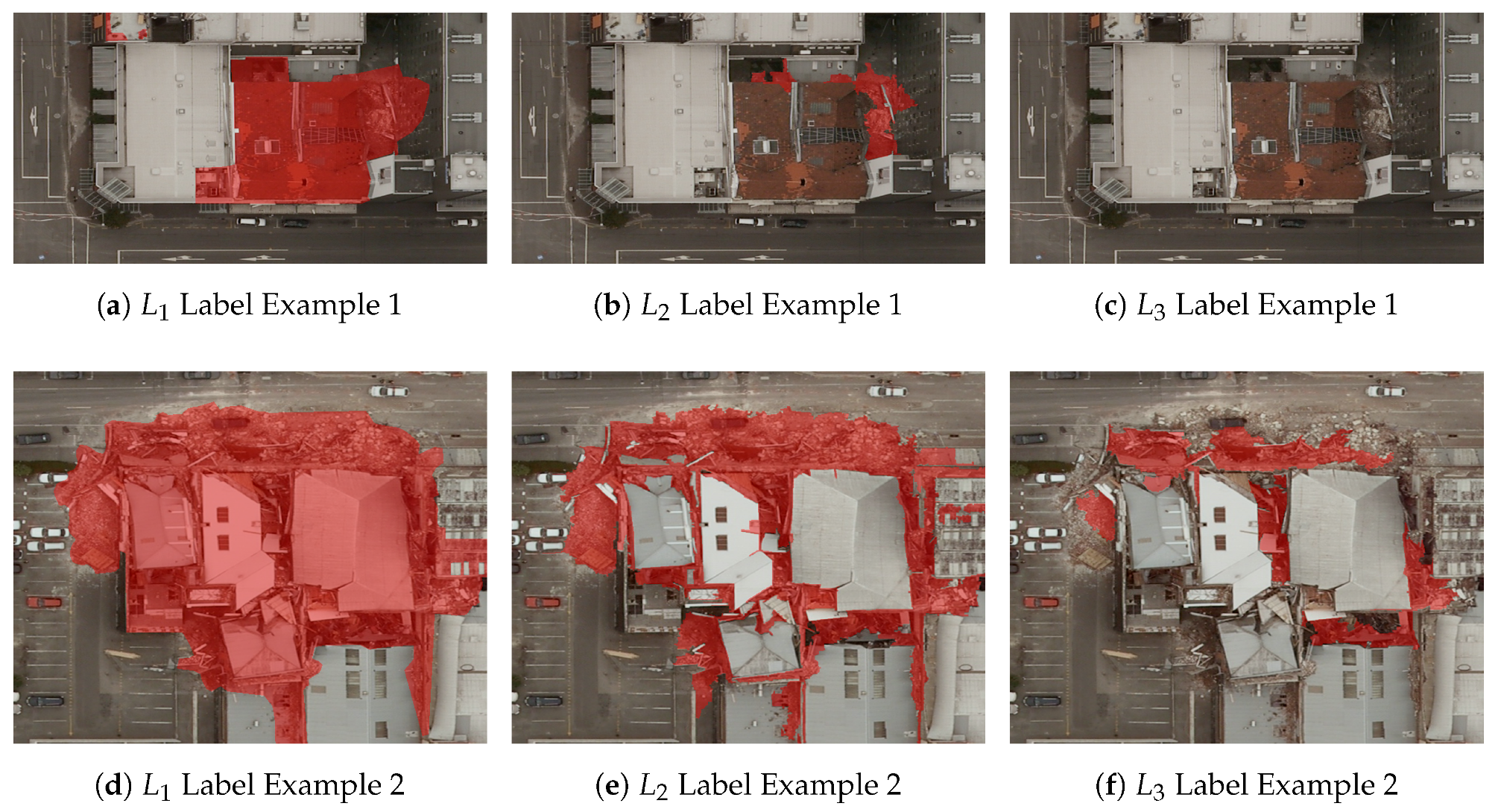
In summary, , and were not only labeled with different tools, but also with different definitions of damage. A closeup of the differing labeling styles can be seen in Figure 7 where the translucent red indicates labeled rubble. In both examples, encircles entire buildings when they are adjacent to rubble. primarily only covers rubble regions. labels nothing in Figure 7c and only labels the very centers of rubble patches in Figure 7f.
We consider to be the best of the three in terms of completeness and cleanliness and use it as a starting point for the simulated label noise. We did not have access to the ground truth for this dataset.
5. Results and Discussion
We present our results on experiments with simulated noise before showing results on experiments with human-labeled training data.
5.1. Experiments with Simulated Noise
Figure 8 shows the effects of increasing levels of NNAR noise types (building and simulated geospatial noise) on both pixel and object-based (GEOBIA) classifiers. We compare both noise types against random noise as a baseline. The horizontal-axis represents the percent of the labeled rubble that is noise. The vertical-axis represents the performance of the classifier trained on the noisy labels. The results are the mean of ten experimental iterations with line width indicating the standard deviation.
We first note that both our pixel-based and GEOBIA classifier are more robust to NAR (random noise) than they are to NNAR (building noise and simulated geospatial noise). The AUC of the GEOBIA classifier’s performance dropped by only percentage points when of the damage class was contaminated. The same classifier’s performance dropped by percentage points under building noise and percentage points under the simulated geospatial label noise. Similarly, the pixel-based classifier’s performance dropped by only percentage points under random noise, but dropped by three and points under building and simulated geospatial noise, respectively.
Under all forms of label noise, the GEOBIA classifier’s performance drops faster than the pixel-based classifier. While the GEOBIA classifier initially outperforms its pixel-based counterpart, classifiers’ performances under geospatial label noise are nearly even when the percentage of noise is slightly over . Although contamination may seem numerically significant, the visual differences lie well within human error. In fact, had nearly -times more rubble pixels labeled than .
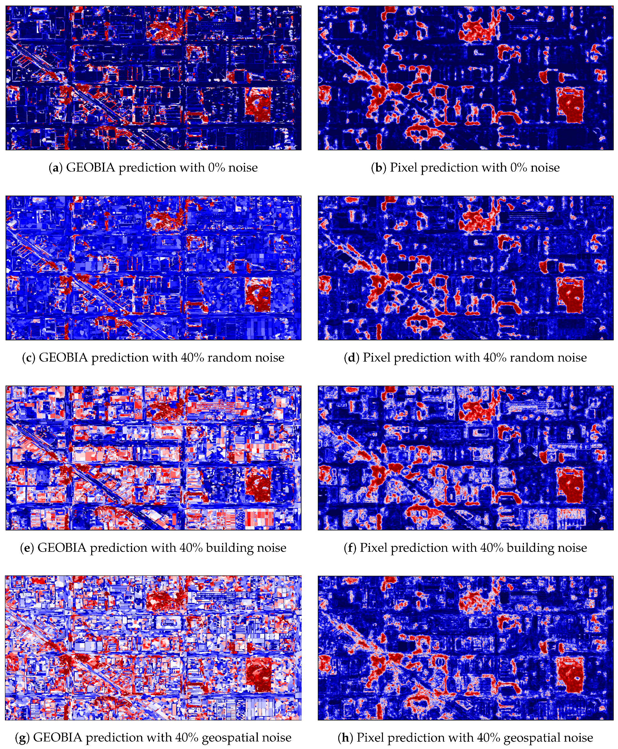
To understand why classifiers are so much more sensitive to building noise, we can analyze the probability heat maps in Figure 9. Dark blue corresponds to a probability of zero, indicating that the classifier is confident that the segment or pixel is non-rubble. Dark red corresponds to a probability of one, indicating that the classifier is confident that the segment or pixel is rubble. White corresponds to a probability close to , indicating that the classifier is unsure of the class of the segment or pixel. Figure 9a shows this heat map when trained on clean labels, and Figure 9c shows this heat map when contaminated with random label noise. Initially, the rubble is primarily correctly identified in dark red, and the rest of the map is confidently not rubble. As more random noise is added, the non-rubble sections uniformly brighten due to increasing uncertainty in their predicted labels. Because all labels increase gradually and uniformly, even when the non-rubble approaches , it is still possible to cleanly threshold the prediction at without losing any true positives or generating new false positives. Figure 9e shows the prediction probabilities when the training data are contaminated with building noise. Because the contaminated segments are solely buildings, the influence on the prediction is concentrated only in these structures. This eliminates the clean threshold separating the damage and non-damage class and generates false positives.
Interestingly, the classifier impacted by simulated geospatial label noise maintains a steady performance for the first 10 to . This could mean that a slightly looser definition of rubble, one that extends spatially farther than our clean labels, would not harm performance. However, as we move past that point, the performance declines at an accelerated rate.
Although the noise progression curves of the simulated geospatial noise appear similar to those of the building noise, the probability heat maps differ greatly. While the building contamination results clearly find only more buildings, the positive predictions for the simulation in Figure 9g are harder to define. Many of the streets are correctly predicted as non-rubble, but the intersections all see spikes in false positives. Some buildings are confidently non-rubble, but others are riddled with incorrect classifications. The prediction is clearly not random, but also defies a simple semantic interpretation. This more realistic noise simulation is just as destructive to the classifier performance, but harder to visually diagnose. The classifier’s extreme degradation is particularly surprising given the relatively minimal and localized contamination as visualized in Figure 5.
The pixel-based heat map of building noise in Figure 9f shows that the pixel-based classifier does not learn to classify buildings nearly as fast as the GEOBIA classifier. Some of the buildings in the pixel heat map show flecks of dark red, but not nearly as uniformly as in the GEOBIA heat map.
Explaining the Noise Resilience of the Px-Based Classifier
To understand why the pixel-based classifier is more robust to noise, we look at the two most prominent differences between the classifiers: the GEOBIA classifier has far more features than the pixel-based classifier, and the pixel-based classifier contains more training data points than the GEOBIA classifier.
Figure 10 shows how these differences impact classifier noise resilience. Figure 10a shows changes in a GEOBIA classifier subjected to building noise when we limit the GEOBIA classifier’s features to only those available to the pixel-based classifier: colors, edge density and the histogram of gradients. This change decreases the overall performance of the classifier, as expected. It also makes the classifier less robust to noise and drops percent compared to the original percent drop. This means that the additional features help with noise resilience and do not explain the difference between the noise resilience of the pixel-based and GEOBIA classifiers.
Figure 10b shows how the pixel-based classifier subjected to building noise changes when we only sample the number of data points available to the GEOBIA classifier, approximately three orders of magnitude smaller than its original size. Under these conditions, the pixel-based classifier does become more sensitive to noise. Its performance drops by percentage points, whereas the original classifier’s performance dropped by only three percentage points. This change accounts for much of the noise resilience disparity between the two classifier paradigms. The smaller training size allows for a larger variance of trees in the random forest because the trees are generated via sampling with replacement. This difference in classifier variance is visible in Figure 10b, where the standard deviation of the classifier using less data is significantly larger. Thus, because GEOBIA classifiers tend to use fewer samples, they are more prone to label contamination in training sets.
5.2. Experiments with Human-Labeled Training Sets
Finally, we compare the performance of the user-labeled training sets , and described in Table 2. We will define the predictions generated by models trained on as .
Because the QGIS labeling was performed with a polygon tool, where polygons do not correspond to the segments used by a GEOBIA classifier, we looked at the composition of labels overlaying the segment in question. If any segment contains more than damage pixels, it is labeled as damage. At larger segment levels, this overlap threshold greatly impacts the training data, but because level 50 segments are small, the difference in prediction based on the threshold is marginal.
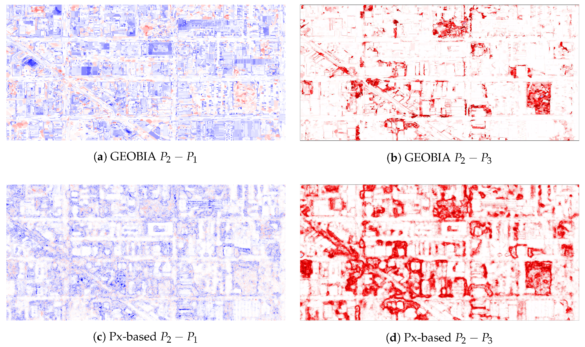
It is difficult to directly compare two labellings because no ground truth labeling exists for the evaluation. However, we can compare how two classifiers trained on two datasets predict new imagery differently by subtracting their probability predictions () as seen in Figure 11. Areas that are red indicate locations where is more likely to label as rubble than . Areas that are blue indicate locations where is more likely to label as rubble than . Areas that are white indicate locations where both and agree.
Figure 11 depicts these probability differences. Figure 11a shows for the GEOBIA classifier. This figure shows a very clear trend that is consistent with our previous simulated results. Because includes more rubble-adjacent buildings, the predictions of building tops shift much more rapidly and threaten the performance of the classifier. Figure 11c shows this same difference, but with the pixel-based classifier. In this probability difference, the buildings are solid white because, even though more buildings have been included in the training, the model’s prediction of them has barely changed. Instead, the rubble sections are darker red toward their centers and light blue toward their edges. This pattern reveals that the building noise has simply broadened ’s rubble predictions and diluted its confidence. In the presence of ’s noisier labeling, the GEOBIA classifier predicted new types of structures, while the pixel-based classifier primarily broadened and became less sure of the structures it had already found. These findings are consistent with the simulated results.
Figure 11b shows . Here, has a more conservative labeling and therefore misses much of the rubble. In this case, as expected, the only difference in prediction is the extent of the prediction. No blue is present, which means that does not predict anything that misses. Instead, simply misses much of the rubble that identifies. A similar trend is seen for the pixel-based classifier in Figure 11d. However, the damage classification of is worse for the pixel-based model than it is for the GEOBIA model, and it therefore predicts more false positives.
6. Conclusions
In this study, we examined a more accurate representation of label noise in remote sensing classification. Our study shows that claims made of classifier resilience to label noise in the machine learning literature do not fully extend to remote sensing. While an object-based classifier does outperform a pixel-based classifier in a clean environment, it must also be trained on a larger area of imagery than is sufficient for the pixel-based classifier. Based on these results, we suggest a few precautionary lessons, especially when dealing with inexperienced labelers.
First, when choosing a classifier, it is important to recognize that the machine learning analyses may need to be reexamined in the context of the specific domain to which they are applied. Although random forest classifiers are known to be robust to label noise, it is worth investigating how label noise appears in remote sensing specifically before accepting theoretical results. In this study, we found that a classifier’s sensitivity to label noise increases in a remote sensing environment. When choosing between pixel-based and GEOBIA classifiers, if label quality is known to be poor and the training region consists of a small geographic area, pixel-based classifiers’ robustness to geospatial label noise may be preferable despite their weaker performance in a clean label environment.
Second, finding or developing effective tools cannot only expedite the labeling process, but also diminish the geospatial label noise that comes with imprecision. Polygon-drawing interfaces may not be precise or efficient enough for some labeling tasks.
Finally, defining a classification task carefully is crucial for high performance results. Broad class definitions are prone to introducing unwanted class-specific noise that may greatly impact classifier predictions. In our own experimentation, performance significantly improved when we refined our objective definition from any damage to just rubble. Both definitions point to the same regions of interest, but the broader term is less separable in the feature space.
These lessons have important implications for the future of crowdsourcing in the remote sensing community. One of the priorities of the Sendai framework for disaster reduction is to enhance disaster preparedness for effective response and “Build Back Better” in terms of recovery, rehabilitation and reconstruction. Earth-observing satellites and crowdsourcing will play a critical role in achieving this principle. The results of this study indicate that while classifier design is crucial, creating an online environment with explicit expectations and carefully crafted tools is perhaps just as important for generating accurate and useful results when trying to harness crowdsourcing to map the impact of extreme events in remotely-sensed images.
Acknowledgments
This material is based on work supported by the National Science Foundation under Grant No. 1300720. Research described in this presentation was carried out at the Jet Propulsion Laboratory, under contract with the National Aeronautics and Space Administration. Copyright 2017. All rights reserved.
Author Contributions
J.F. did the primary research, including the design and execution of experiments, development of the web tool, results analysis and paper writing. U.R. supervised the research and edited the paper. J.B. provided data and labels for experimentation. U.R., J.B., T.O. and T.C.H. provided feedback on the paper’s experimentation and write-up.
Conflicts of Interest
The authors declare no conflict of interest.
References
- Kaya, G.; Taski, K.; Musaoglu, N.; Ersoy, O. Damage assessment of 2010 Haiti earthquake with post-earthquake satellite image by support vector selection and adaptation. Photogramm. Eng. Remote Sens. 2011, 77, 1025–1035. [Google Scholar] [CrossRef]
- Li, P.; Xu, H.; Liu, S.; Guo, J. Urban building damage detection from very high resolution imagery using one-class SVM and spatial relations. In Proceedings of the IEEE International, Geoscience and Remote Sensing Symposium, Cape Town, South Africa, 12–17 July 2009; pp. V-112–V-114m. [Google Scholar]
- McMurren, J.; Verhults, S.; Young, A. New Zealand’s Christchurch Earthquake Clusters. Open Data’s Impac. 2016. Available online: http://odimpact.org/case-new-zealands-christchurch-earthquake-clusters.html (accessed on 20 July 2016).
- Huynh, A.; Eguchi, M.; Lin, A.Y.-M.; Eguchi, R. Limitations of crowdsourcing using the EMS-98 scale in remote disaster sensing. In Proceedings of the 2014 IEEE Aerospace Conference, Big Sky, MT, USA, 1–8 March 2014; pp. 1–8. [Google Scholar]
- Corbane, C.; Saito, K.; Dell’Oro, L.; Bjorgo, E.; Gill, S.P.D.; Piard, B.E.; Huyck, C.K.; Kemper, T.; Lemoine, G.; Spence, R.J.S.; et al. A comprehensive analysis of building damage in the January 12, 2010 Mw7 Haiti earthquake using high-resolution satellite and aerial imagery. Photogramm. Eng. Remote Sens. 2011, 77, 997–1009. [Google Scholar] [CrossRef]
- Clark, L. How Nepal’s Earthquake Was Mapped in 48 hours. Wired. 28 April 2015. Available online: http://www.wired.co.uk/article/mapping-nepal-after-the-earthquake (accessed on 29 July 2016).
- See, L.; Mooney, P.; Foody, G.; Bastin, L.; Comber, A.; Jacinto, E.; Steffen, F.; Kerle, N.; Jiang, B.; Laakso, M.; et al. Crowdsourcing, Citizen Science or Volunteered Geographic Information? The Current State of Crowdsourced Geographic Information. ISPRS Int. J. Geo-Inf. 2016, 5, 55. [Google Scholar] [CrossRef]
- Bialas, J.; Oommen, T.; Rebbapragada, U.; Levin, E. Object-based classification of earthquake damage from high-resolution optical imagery using machine learning. J. Appl. Remote Sens. 2016, 10, 036025. [Google Scholar] [CrossRef]
- Ghimire, B. An Evaluation of Bagging, Boosting, and Random Forests for Land-Cover Classification in Cape Cod, Massachusetts, USA. GISci. Remote Sens. 2012, 49, 623–643. [Google Scholar] [CrossRef]
- Gislason, P. Random Forests for land cover classification. Patter Recognit. Lett. 2006, 27, 294–300. [Google Scholar] [CrossRef]
- Blaschke, T.; Hay, G.; Kelly, M.; Lang, S.; Hofmann, P.; Addink, E.; Feitosa, R.; van der Meer, F.; van der Werff, H.; van Coillie, G.; et al. Geographic Object-Based Image Analysis-Towards a new paradigm. ISPRS J. Photogramm. Remote Sens. 2014, 87, 180–191. [Google Scholar] [CrossRef] [PubMed]
- Blaschke, T.; Lang, S.; Lorup, E.; Zeil, P. Object-oriented image processing in an integrated GIS/remote sensing environment and perspectives for environmental applications. Environ. Inf. Plan. Politics 2000, 2, 555–570. [Google Scholar]
- Rodriguesz-Galiano, V.; Ghimire, B.; Rogan, J.; Rigol-Sanchez, J. An assessment of the effectiveness of a random forest classifier for land-cover classification. ISPRS J. Photogramm. Remote Sens. 2012, 67, 93–104. [Google Scholar] [CrossRef]
- Simard, M.; Saatchi, S.S.; De Grandi, G. The use of decision tree and multiscale texture for classification of JERS-1 SAR data over tropical forest. IEEE Trans. Geosci. Remote Sens. 2000, 38, 2310–2321. [Google Scholar] [CrossRef]
- Marpu, P.R. Geographic Object-Based Image Analysis. Ph.D. Thesis, The Faculty of Geosciences, Geo-Engineering and Mining of the Technische Universitat Bergakademie, Freiberg, Germany, 2009. [Google Scholar]
- Frénay, B.; Verleysen, M. Classification in the presence of label noise: A survey. IEEE Trans. Neural Netw. Learn. Syst. 2014, 25, 845–869. [Google Scholar] [CrossRef] [PubMed]
- Chhikara, R.; McKeon, J. Linear Discriminant Analysis with Misallocation in Training Samples. J. Am. Stat. Assoc. 1984, 79, 899–906. [Google Scholar] [CrossRef]
- Foody, G.M.; Pal, M.; Rocchini, D.; Garzon-Lopez, C.X.; Bastin, L. The Sensitivity of Mapping Methods to Reference Data Quality: Training Supervised Image Classifications with Imperfect Reference Data. ISPRS Int. J. Geo-Inf. 2016, 5, 199. [Google Scholar] [CrossRef]
- Foody, G.M. The impact of imperfect ground reference data on the accuracy of land cover change estimation. Int. J. Remote Sens. 2009, 30, 3275–3281. [Google Scholar] [CrossRef]
- Foody, G.M. Assessing the accuracy of the land cover change with imperfect ground reference data. Remote Sens. Environ. 2010, 114, 2271–2285. [Google Scholar] [CrossRef]
- Land Information New Zealand. Christchurch Earthquake Imagery. Available online: http://www.linz.govt.nz/land/maps/linz-topographic-maps/imagery-orthophotos/christchurch-earthquake-imagery (accessed on 3 September 2013).
- Breiman, L. Random Forests. Mach. Learn. 2001. [Google Scholar] [CrossRef]
- Baatz, M.; Schäpe, A. Multiresolution segmentation: An optimization approach for high quality multi-scale image segmentation. XII Angew. Geogr. Informationsverarbeitung 2000, XII, 12–23. [Google Scholar]
- Lowe, G. Distinctive Image Features from Scale-Invariant Keypoints. Int. J. Comput. Vis. 2004, 60, 91–110. [Google Scholar] [CrossRef]
- Bradski, G. The OpenCV Library. Dr. Dobb’s. Available online: http://www.drdobbs.com/open-source/the-opencv-library/184404319 (accessed on 27 April 2017).
- Van der Walt, S.; Schönberger, J.L.; Nunez-Iglesias, J.; Boulogne, F.; Warner, J.D.; Yager, N.; Gouillart, E.; Yu, T. Scikit-image: Image processing in Python. PeerJ 2014, 2, e453. [Google Scholar] [CrossRef] [PubMed]
- Definiens Developer Reference Book XD 2.0.4. Definiens AG, 2012. Available online: http://www.imperial.ac.uk/media/imperial-college/medicine/facilities/film/Definiens-Developer-Reference-Book-XD-2.0.4.pdf (accessed on 1 August 2017).
Figure 1.
Annotations of the same destroyed building by two users using different labeling tools and methodologies. (a) User 1 was tasked with marking “damage” and included an intact roof in the training data, whereas in (b) User 2 limited annotation to rubble only. User 1’s annotation would confuse a rubble classifier.

Figure 2.
This image superimposes the attempts of five individuals at labeling rubble. Bright red indicates that all labelers believed the area was damage, while dark red indicates that only one labeler did. Regions in which labelers tend to disagree happen in close geospatial proximity to regions in which all labelers agree.
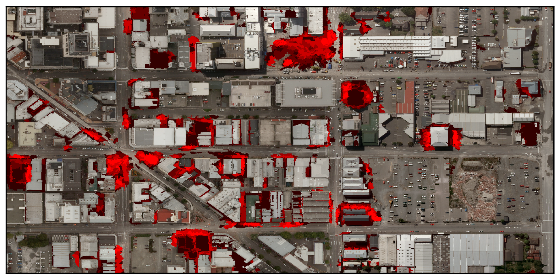
Figure 3.
(a) Region of study in New Zealand. (b) A top-bottom concatenation of Tiles 1-0003-0003 and 1-0003-0002 where 1-0003-0003 (top) contains the two tree-lined square enclosures and 1-0003-0002 (bottom) features a large rubble-filled X-shaped intersection and a construction quarry on the bottom right.
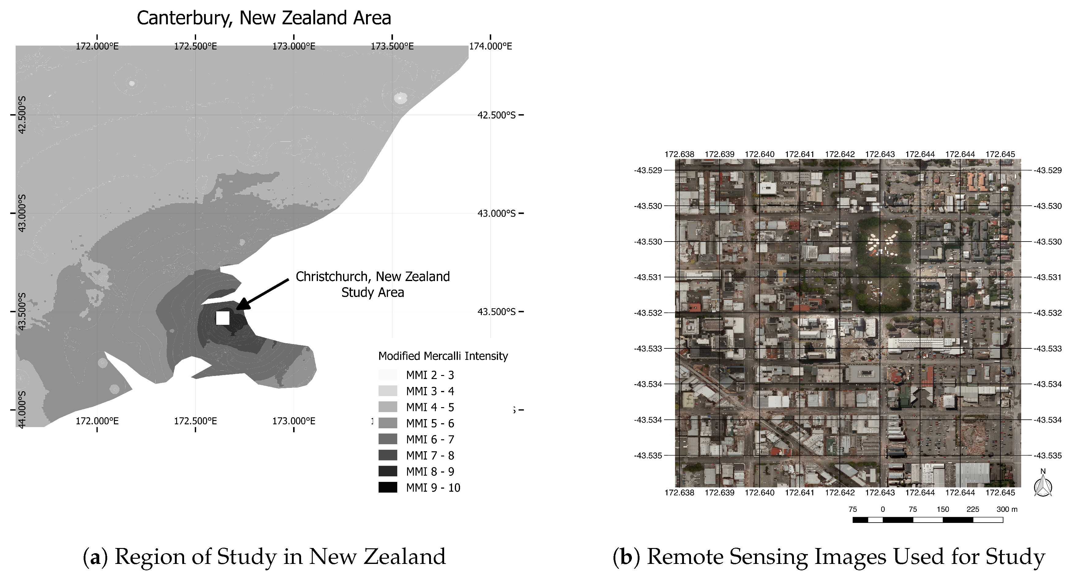
Figure 4.
The 24 features with the highest feature importance values to the GEOBIA classifier.
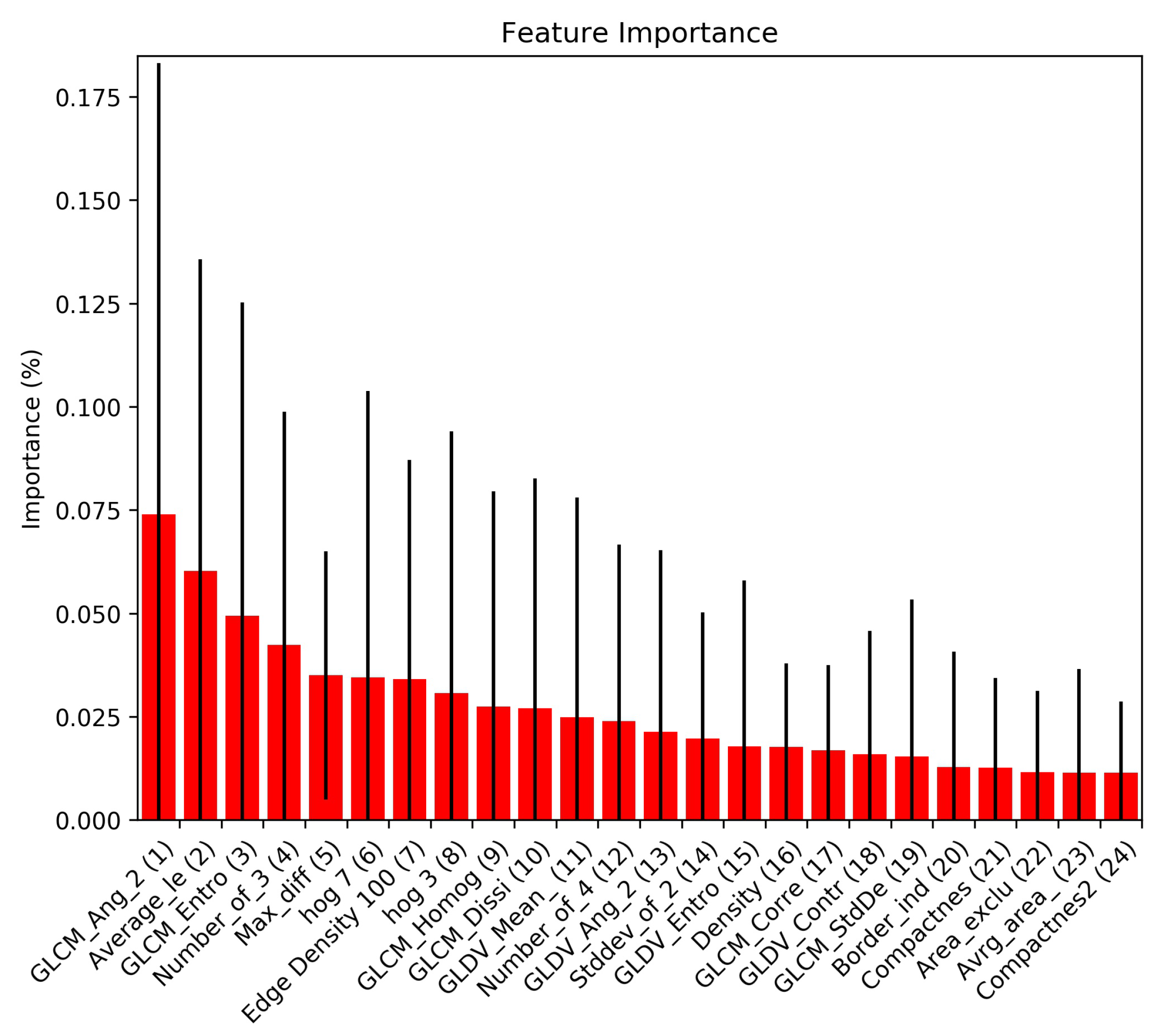
Figure 5.
Simulated geospatial label noise using morphological dilation. Red pixels indicate rubble labels: (a) 0% simulated noise; (b) 40% simulated noise.
Figure 5.
Simulated geospatial label noise using morphological dilation. Red pixels indicate rubble labels: (a) 0% simulated noise; (b) 40% simulated noise.
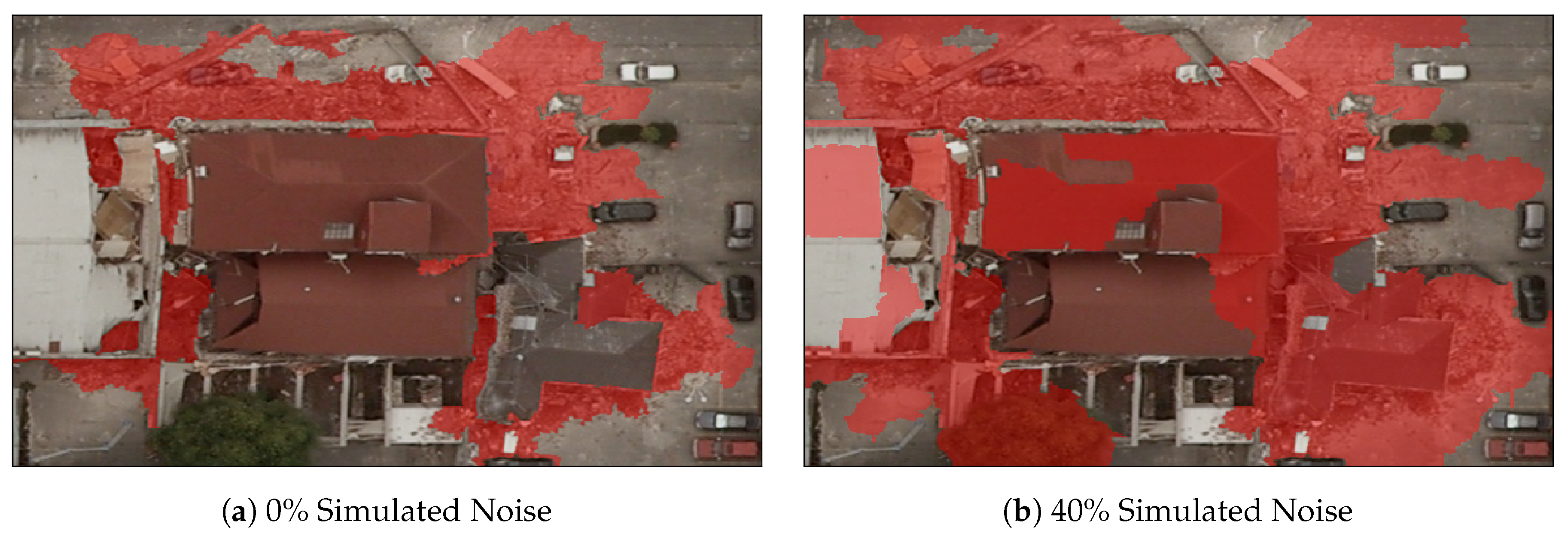
Figure 6.
A comparison of labeling tools. (a) Labeling rubble using QGIS’s built-in polygon tool. (b) The editing mode of our custom labeling tool. The user labels segments via clicking and dragging her/his mouse. (c) A zoomed out view of our custom labeling tool. A tile outlined in green indicates that the user has already labeled it.
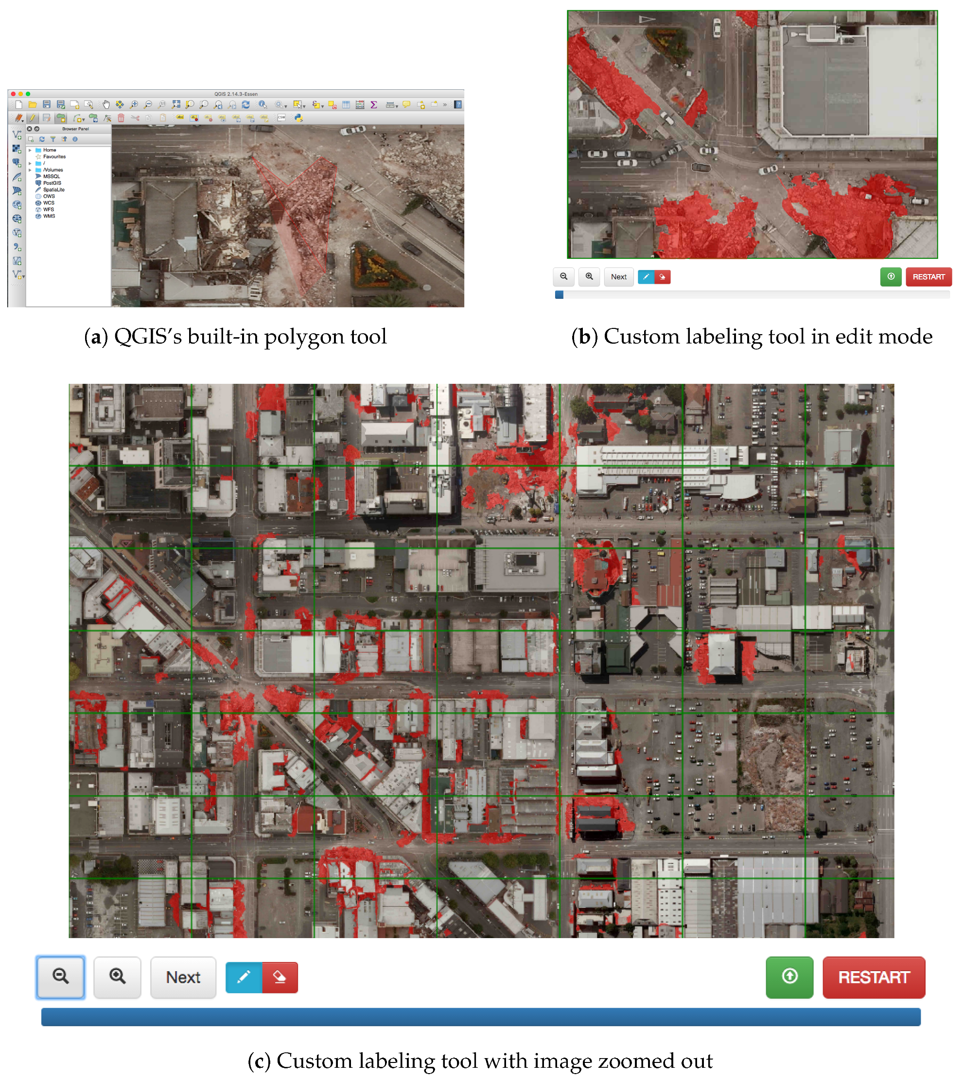
Figure 7.
Annotations of the same destroyed building. The translucent red indicates labeled rubble. The left labels, , were drawn with polygons in QGIS. The middle labels, , were drawn with a custom labeling tool. The right labels, , were labeled using eCognition.
Figure 7.
Annotations of the same destroyed building. The translucent red indicates labeled rubble. The left labels, , were drawn with polygons in QGIS. The middle labels, , were drawn with a custom labeling tool. The right labels, , were labeled using eCognition.

Figure 8.
We measure classification performance (in terms of AUC) under increasing amounts of label noise. Object-based classifiers perform better at low noise levels, but are less resilient to label noise. The line width indicates the standard deviation of the result. (a) Building noise. (b) Geospatial noise vs. random noise.
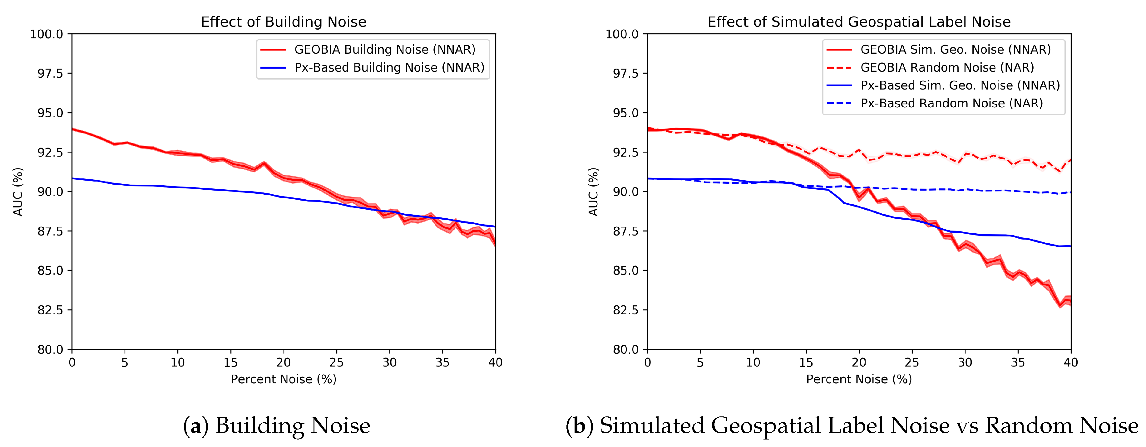
Figure 9.
Probability heat maps with noise. Dark blue indicates that the classifier is confident that the segment or pixel is non-rubble. Dark red indicates that the classifier is confident that the segment or pixel is damage. White indicates that the classifier is unsure of the class of the segment or rubble. (a) GEOBIA prediction with 0% noise. (b) Pixel prediction with 0% noise. (c) GEOBIA prediction with 40% random noise. (d) Pixel prediction with 40% random noise. (e) GEOBIA prediction with 40% building noise. (f) Pixel prediction with 40% building noise. (g) GEOBIA prediction with 40% geospatial noise. (h) Pixel prediction with 40% geospatial noise.

Figure 10.
A test of two hypotheses: (a) What is GEOBIA’s performance when limited to the features used by the pixel-based (Px-based) classifier? (b) What is the Px-based performance when limited to the same number of training samples as GEOBIA?
Figure 10.
A test of two hypotheses: (a) What is GEOBIA’s performance when limited to the features used by the pixel-based (Px-based) classifier? (b) What is the Px-based performance when limited to the same number of training samples as GEOBIA?
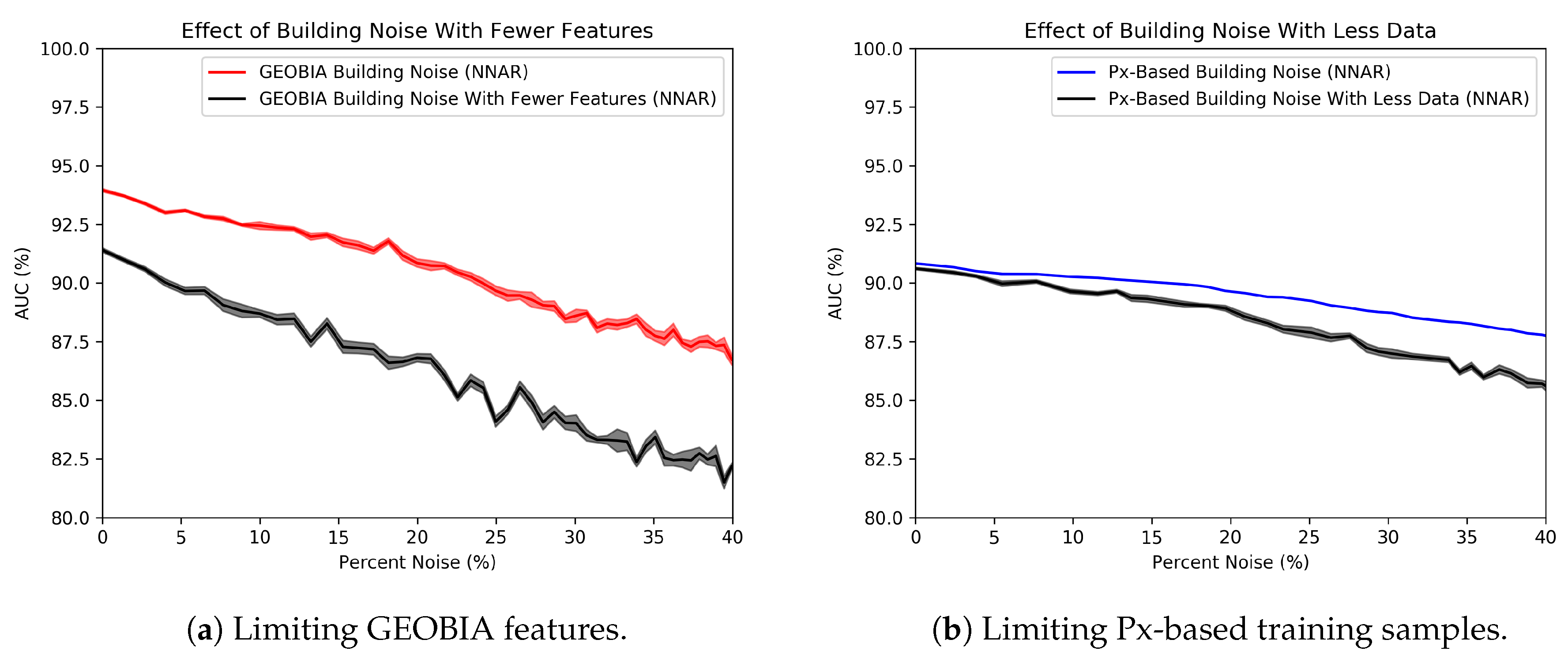
Figure 11.
Prediction differences resulting from the use of , and . For any , areas that are red indicate locations where is more likely to label as rubble than . Areas that are blue indicate locations where is more likely to label as rubble than . Areas that are white indicate locations where both and agree. (a) GEOBIA . (b) GEOBIA . (c) Px-based . (d) Px-based .

Table 1.
Object-based features calculated per segment using eCognition software. These features are defined in [27].
Table 1.
Object-based features calculated per segment using eCognition software. These features are defined in [27].
| Class | Features |
|---|---|
| Spectral | Brightness, Mean Value, Standard Deviation, Max. Diff., Hue, Saturation, Intensity |
| Texture | GLCM Homogeneity, GLCM Contrast, GLCM Dissimilarity, GLCM Entropy, GLCM Angular 2nd Momentum, GLCM Mean, GLCM Std. Dev., GLCM Correlation, GLDV Angular 2nd Momentum, GLDVEntropy |
| Shape | Extent Area, Border Length, Length, Length/Thickness, Length/Width, Number of Pixels, Thickness, Volume, Width |
| Shape Asymmetry, Border Index, Compactness, Density, Elliptic Fit, Main Direction, Radius of Largest Enclosed Ellipse, Radius of Smallest Enclosed Ellipse, Rectangular Fit, Roundness, Shape Index | |
| Based on Polygons Area (excluding inner polygons), Area (including inner polygons), Average Length of Edges (Polygon), Compactness (Polygon), Length of Longest Edge (Polygon), Number of Edges (Polygon), Number of Inner Objects (Polygon), Perimeter (Polygon), Polygon Self-Intersection (Polygon), Std. Dev. Of Length of Edges | |
| Based on Skeletons Average Branch Length, Average Area Represented by Segments, Curvature/Length (Only Main Line), Degree of Skeleton Branching, Length of Main Line (No Cycles), Length of Main Line (Regarding Cycles), Length/Width (Only Main Line), Maximum Branch Length, Number of Segments, Std. Dev. Curvature (Only Main Line), Std. Dev. of Area Represented by Segments, Width (Only Main Line) |
Table 2.
Human-labeled datasets.
| Dataset | Labeling Tool | Methodology |
|---|---|---|
| QGIS Polygon Drawing | Full image labeled. Tendency toward over-labeling rubble. | |
| Web-based Segment Labeling (scale = 50) | Full image labeled by segment. Considered the cleanest of three. | |
| eCognition Segment Labeling (scale = 25) | Partial image labeled. Some rubble areas omitted from training. |
© 2017 by the authors. Licensee MDPI, Basel, Switzerland. This article is an open access article distributed under the terms and conditions of the Creative Commons Attribution (CC BY) license (http://creativecommons.org/licenses/by/4.0/).
Share and Cite
MDPI and ACS Style
Frank, J.; Rebbapragada, U.; Bialas, J.; Oommen, T.; Havens, T.C. Effect of Label Noise on the Machine-Learned Classification of Earthquake Damage. Remote Sens. 2017, 9, 803. https://doi.org/10.3390/rs9080803
AMA Style
Frank J, Rebbapragada U, Bialas J, Oommen T, Havens TC. Effect of Label Noise on the Machine-Learned Classification of Earthquake Damage. Remote Sensing. 2017; 9(8):803. https://doi.org/10.3390/rs9080803
Chicago/Turabian StyleFrank, Jared, Umaa Rebbapragada, James Bialas, Thomas Oommen, and Timothy C. Havens. 2017. "Effect of Label Noise on the Machine-Learned Classification of Earthquake Damage" Remote Sensing 9, no. 8: 803. https://doi.org/10.3390/rs9080803
Note that from the first issue of 2016, this journal uses article numbers instead of page numbers. See further details here.