Estimation of Fugacity of Carbon Dioxide in the East Sea Using In Situ Measurements and Geostationary Ocean Color Imager Satellite Data


1
School of Urban and Environmental Engineering, Ulsan National Institute of Science and Technology (UNIST), Ulsan 44919, Korea
2
East Sea Research Institute, Korea Institute of Ocean Science and Technology, Uljin 36315, Korea
3
Korea Institute of Ocean Science and Technology, Ansan 15627, Korea
*
Author to whom correspondence should be addressed.
Remote Sens. 2017, 9(8), 821; https://doi.org/10.3390/rs9080821
Submission received: 24 May 2017
/
Revised: 1 August 2017
/
Accepted: 8 August 2017
/
Published: 10 August 2017
(This article belongs to the Section Ocean Remote Sensing)
Abstract
:The ocean is closely related to global warming and on-going climate change by regulating amounts of carbon dioxide through its interaction with the atmosphere. The monitoring of ocean carbon dioxide is important for a better understanding of the role of the ocean as a carbon sink, and regional and global carbon cycles. This study estimated the fugacity of carbon dioxide (ƒCO2) over the East Sea located between Korea and Japan. In situ measurements, satellite data and products from the Geostationary Ocean Color Imager (GOCI) and the Hybrid Coordinate Ocean Model (HYCOM) reanalysis data were used through stepwise multi-variate nonlinear regression (MNR) and two machine learning approaches (i.e., support vector regression (SVR) and random forest (RF)). We used five ocean parameters—colored dissolved organic matter (CDOM; <0.3 m−1), chlorophyll-a concentration (Chl-a; <21 mg/m3), mixed layer depth (MLD; <160 m), sea surface salinity (SSS; 32–35), and sea surface temperature (SST; 8–28 °C)—and four band reflectance (Rrs) data (400 nm–565 nm) and their ratios as input parameters to estimate surface seawater ƒCO2 (270–430 μatm). Results show that RF generally performed better than stepwise MNR and SVR. The root mean square error (RMSE) of validation results by RF was 5.49 μatm (1.7%), while those of stepwise MNR and SVR were 10.59 μatm (3.2%) and 6.82 μatm (2.1%), respectively. Ocean parameters (i.e., sea surface salinity (SSS), sea surface temperature (SST), and mixed layer depth (MLD)) appeared to contribute more than the individual bands or band ratios from the satellite data. Spatial and seasonal distributions of monthly ƒCO2 produced from the RF model and sea-air CO2 flux were also examined.
1. Introduction
Carbon dioxide, one of the greenhouse gases, has significantly increased since the industrial revolution due to economic and population growth. Increase of carbon dioxide concentration in the atmosphere accelerates global warming, which is directly related with on-going climate change. Climate change has brought significant impacts on human society and the natural environment all over the world, in such ways as increasing extreme weather events and a rise in sea levels [1]. The ocean contains fifty times more carbon dioxide than the atmosphere, and twenty times more than terrestrial ecosystems. Although the substantial amount of carbon dioxide in the atmosphere is absorbed into the oceans, approximately half of anthropogenic carbon dioxide remains in the atmosphere, increasing its concentration [2]. Since the ocean acts as a buffer for carbon dioxide uptake, temporal and spatial changes of the sea-air carbon dioxide flux are crucial to understanding the global carbon cycle [3].
The increasing absorption of carbon dioxide from the atmosphere can result in huge damage to marine organisms [4]. When the carbon dioxide dissolves in seawater, it becomes carbonic acid and has a negative effect on biochemical functions of organisms, in particular, calcareous ones, such as lime, coral algae, clams, and oysters, with their shells composed of calcium carbonate ([5] and references therein, for example). Accumulated carbon dioxide in the ocean accelerates global warming and climate change by decreasing the capacity of the ocean that absorbs carbon dioxide from the atmosphere. Consequently, quantifying the distribution of ocean carbon dioxide is crucial in order to better understand the ocean carbon sink [6]. However, there has been limited exploration of ocean carbon dioxide around East Asia, especially in the East Sea located between Korea and Japan.
In situ field observations are relatively limited over the ocean because of technical and financial problems [6]. In addition, in situ measurements are not typically continuous in the spatiotemporal domain. Satellite remote sensing can be a good alternative to this as satellite sensors collect data over vast areas at high temporal resolution (~hours). Satellite data can be used to estimate various ocean parameters including chlorophyll-a concentration (Chl-a), sea surface temperature (SST), and colored dissolved organic materials (CDOM), which are related to the distribution of carbon dioxide in the ocean.
In this study, we used multi-sensor satellite data and in situ measurements to quantify carbon dioxide over the East Sea of Korea. This study focuses on the fugacity of carbon dioxide (ƒCO2) in surface seawater, in order to examine ocean carbon dioxide. Fugacity is expressed in Pascals or in atmospheres, the same unit as is used with partial pressure. Since it is difficult to retrieve pressure (or fugacity) of carbon dioxide directly from satellite reflectance data, it is necessary to use satellite-derived ocean parameters that are related to carbon dioxide concentration [7]. Many studies have suggested that SST and Chl-a are the important parameters for estimating the partial pressure of carbon dioxide [8,9,10,11,12,13,14,15,16,17,18,19]. The capacity of gas solubility is highly related to SST. SST also affects other carbon pumps, which are physical transport and biological photosynthesis and respiration [20]. SST could act as an indication of cooler upwelling water by vertical mixing [7]. In addition, sea surface salinity (SSS) [6,7,8,11,12,15], mixed layer depth (MLD) [10,11,16], CDOM [21], and wind speed [6,16,21] were used to quantify the partial pressure of carbon dioxide in the ocean. SSS also shows the variability of carbon dioxide by expressing the mixing between seawater and freshwater [7]. SSS can determine the characteristics of surface seawater carbon dioxide not determined by other ocean parameters (i.e., SST, MLD, and biological variables) as water mass tracer and water parcel history [22]. MLD is defined as the depth of the vertical mixing process of the ocean. The bottom layer of seawater has a high concentration of dissolved inorganic carbon, which can come up to the surface through the process, resulting in ƒCO2 increases [23,24]. CDOM and Chl-a are controlled by organisms that produce O2 and consume CO2. Active photosynthesis decreases surface water ƒCO2 [23,25,26,27]. Temperature is related to seasonal thermal balance [7].
The East Sea, surrounded by Korean peninsula, Japan, and Russia, is a mid-latitude marginal sea with average depth of about 1750 m. It is connected to the western North Pacific through the Korea, Tsugaru, Soya/La Pérouse, and Tatar Straits. The inflow through the Korea Strait that brings warm and salty water, and the outflow through the Tsugaru, Soya/La Pérouse are mainly confined to about upper 150 m. Below the upper level, there is a thermohaline circulation due to deep convection occurring in the northern part of East Sea [28,29]. Deep convection carries anthropogenic carbon dioxide into the East Sea, making a large reservoir for carbon dioxide. The specific column inventory of anthropogenic carbon dioxide in the East Sea is two or three times greater than that of the North Pacific, which results in a great change in the carbonate chemistry of the sea through the large accumulation of carbon dioxide [23]. Within the East Sea, ƒCO2 varies even over a small area due to environmental variations [30]. In response to the increase in the atmospheric CO2 concentration, ƒCO2 in the East Sea steadily increased between 1995 and 2010 [20]. A numerical model with ocean carbon chemistry suggests that the inflow into the East Sea could also contribute to a change in ƒCO2 [31]. Considering these environments, quantifying ƒCO2 is crucial for monitoring carbon flux in the East Sea and improving our understanding of the regional carbon cycle. However, there have been only a few studies analyzing the carbon dioxide in the East Sea using in situ data [20,23,30]. Park et al. [32] constructed a neural network model to estimate pCO2 in the East Sea based on satellite-derived SST and Chl-a and in situ pCO2 data from 2003 to 2012. The variability of pCO2 was large due to high primary production and mesoscale eddies, and the relationship between pCO2 and SST was higher than Chl-a [32].
Most of the studies mentioned above estimated the pressure of ocean carbon dioxide using in situ and satellite data through statistical approaches, such as simple linear and multiple linear regression. Such linear approaches might not work well for the nonlinear behavior of carbon dioxide over the ocean with a dynamic spatiotemporal environment. More advanced algorithms that can handle the nonlinear behavior are required to examine the relationship between ocean carbon dioxide and ocean related parameters [33]. In the field of remote sensing, recently adopted machine learning approaches or nonlinear analyses, may be able to effectively model the pressure of ocean carbon dioxide. These techniques include various neural networks including self-organizing maps (SOM) [6,14,15,20,32,34,35], mechanistic nonlinear models [13], principal component analysis [9], mechanistic semi-analytic algorithms [7], and quadratic polynomial regression [9]. However, generalization of the empirical modeling approaches from one area to different areas is still challenging.
Most of the studies mentioned above used polar orbiting satellite sensors (especially, Moderate Resolution Imaging Spectroradiometer (MODIS)). We used Geostationary Ocean Color Imager (GOCI) satellite sensor, which has higher spatial and temporal resolutions than MODIS. This is the first study to estimate the surface seawater ƒCO2 using GOCI satellite data.
The objectives of this study were (1) to estimate surface seawater ƒCO2 in the East Sea of Korea using satellite data and in situ measurements based on multi-variate nonlinear regression (MNR) and machine learning approaches, and (2) to examine ocean parameters contributing to ƒCO2 estimation, and (3) investigate the spatial and temporal variation of surface seawater ƒCO2 and sea-air CO2 flux over the East Sea using satellite data. Two machine learning approaches including support vector regression (SVR) and random forest (RF) were used in this study. MNR, recently applied in a study [9] to estimate pCO2, was used for comparison with the two machine learning approaches.
2. Data
2.1. In Situ Data
In situ measurements for this study were provided by the Korea Institute of Ocean Science and Technology (KIOST). KIOST conducted several field surveys (May 2014; August 2014; March 2015; April 2015; August 2015; October 2015; November 2015) in the East Sea and provided in situ data measured every minute. Each point data contains information about the date/time, location (latitude and longitude), SST (°C), SSS, and ocean ƒCO2 (μatm).
In the LI-COR (LI-COR Biosciences, Lincoln, NE, USA) LI-7000 mode, a non-dispersive infrared analysis instrument was used to measure concentrations of carbon dioxide in the atmosphere and ocean by the standard operating procedure (SOP) [36]. The underway CO2 data obtained from the non-dispersive infrared analyzer were calibrated using three non-zero standard gases with known CO2 concentrations every three hours. SST and SSS were measured using a Sea-Bird Electronics 45 Micro TSG thermosalinograph (Sea-Bird Electronics Inc., Bellevue, WA, USA). It measures sea surface conductivity and SST in real time by passing seawater through the pump, and also computes SSS. Surface seawater was pumped aboard from a 2-m depth and a showerhead type equilibrator was used. The underway system was operated on a cycle consisting of three standard gases, measurements of air, and measurements of a headspace equilibrated with flowing seawater. Air and seawater measurements were conducted at a 1-min interval. The system measured the mole fraction of CO2 in dry air (xCO2), which was converted into CO2 fugacity by correcting for the non-ideality of the gas and the water vapor level, as outlined in [37]. All post-cruise calculations of ƒCO2 including temperature correction were done using the methods described in [37]. The maximum ƒCO2 in summer (August 2014) is higher than the other seasons due to warming of surface seawater (Figure 1; Table 1 and Table 2). Warming of surface seawater increases ƒCO2 thermodynamically [38]. Surface seawater ƒCO2 is higher in fall than spring because of a higher SST and deeper MLD.
2.2. GOCI Imagery
The Geostationary Ocean Color Imager (GOCI), launched in June 2010, is the first geostationary ocean color observation satellite sensor in the world. GOCI collects data hourly for 8 h per day from 9 a.m. to 4 p.m. in local time at six visible (centered at 412 nm, 443 nm, 490 nm, 555 nm, 660 nm, and 680 nm) and two near-infrared bands (centered at 745 nm and 865 nm) at 500 m resolution. It covers 2500 km × 2500 km square around the Korean peninsula, East China, and Japan (Figure 1). GOCI provides three basic products including the concentrations of Chl-a, suspended sediment, and CDOM, which are downloadable from the Korea Ocean Satellite Center (KOSC) website [39] free charge. This study used Chl-a and CDOM products (Table 1), which are related to the biochemical processes and carbon cycle on the ocean surface. Band reflectance (Rrs) data at four visible bands (bands 1–4; Table 3) among the eight bands were used in this study because most pixels in red and NIR bands have very low reflectance close to 0. Details of the products are found in the KOSC website [40].
2.3. HYCOM Imagery
The HYbrid Coordinate Ocean Model + NRL Coupled Ocean Data Assimilation (HYCOM + NCODA) system provides reanalyzed ocean data based on multiple satellite data and in situ measurements through partnerships with various academic, governmental, and commercial entities, such as the Florida State University Center for Ocean-Atmospheric Prediction Studies (FSU/COAPS), the Naval Research Laboratory/Stennis Space Center (NRL/STENNIS), the National Oceanographic and Atmospheric Administration (NOAA), and Planning Systems Inc. (Reston, VA, USA). Among many variables that HYCOM provides, we used the daily 1/12 degree (around 8.3 km) MLD, SST, and SSS products (Table 1), which were downloaded from the HYCOM + NCODA homepage [41].
2.4. NOAA Greenhouse Gas Marine Boundary Layer Reference
NOAA Greenhouse Gas Marine Boundary Layer (MBL) reference provides surface xCO2 data based on in situ measurements for all over the ocean, which is provided from the NOAA Earth System Research Laboratory (ESRL) carbon cycle cooperative global air sampling network [42]. Surface xCO2 data was used to calculate atmosphere ƒCO2 to analyze carbon sink or source in the East Sea. They provide weekly data at intervals of 0.05 times the sine of latitude, and it was downloaded from the NOAA ESRL Greenhouse Gas MBL reference homepage [43].
2.5. European Reanalysis of (ERA-) Interim Data
European Centre for Medium-Range Weather Forecasts (ECMWF) provides ERA-Interim data, which is global atmospheric reanalysis data since 1979 based on data assimilation [44]. ERA-Interim data include various variables related with atmospheric conditions. We used daily 0.125 degree mean sea level pressure, and 10 m U and V wind components to calculate atmosphere ƒCO2 and sea-air CO2 flux. ERA-Interim daily data were downloaded from the ECMWF homepage [45]
3. Methodology
3.1. Experimental Schemes
In this study, five major ocean parameters and individual band reflectance (Rrs) data were used to estimate ƒCO2 in surface seawater from GOCI satellite products and in situ measurements We used ocean parameters (SST, SSS, MLD, CDOM, and Chl-a), as in the existing literature, and additionally individual band reflectance and band ratio data as input parameters. Satellite-derived ocean parameters are produced using band reflectance data, sometimes causing high uncertainty, especially near coastal areas. Band reflectance data and their ratios were considered because there is a chance that satellite-derived CDOM and Chl-a products might not effectively reflect biological processes in the East Sea.
In this study, samples, which spatiotemporally matched satellite data, were used to estimate ƒCO2. Some samples were excluded due to cloud cover in the corresponding satellite data, and, when multiple samples were located within one pixel, they were averaged. While in situ data were measured every minute, satellite data were collected either every hour between 9 a.m. and 4 p.m. for GOCI at 500 m spatial resolution. Thus, in situ samples were selected considering the collection times and the spatial resolution of satellite data. HYCOM data were resampled at 500 m, the same pixel size with GOCI, using bilinear interpolation. Samples were divided into two groups: eighty percent of the samples were randomly selected and used to train machine learning algorithms, while the remaining samples (twenty percent of the samples) were used to validate the models to estimate ƒCO2.
We used four band reflectance data (excluding red and NIR bands; Table 3) and their ratios, and ocean parameters (CDOM, Chl-a, MLD, SSS, and SST) as input parameters to develop machine learning models to estimate ƒCO2 in surface seawater. The total number of samples was for 843 (673 for calibration and 170 for validation). SST, SSS, and MLD (from HYCOM) and visible (i.e., blue and green) band reflectance (Rrs), their ratios, CDOM, and Chl-a (from GOCI) were used to develop machine learning models for surface seawater ƒCO2 estimation. Then, the developed models were applied to GOCI satellite band reflectance, their ratios, CDOM, Chl-a, HYCOM MLD, SSS, and SST images to examine the spatiotemporal patterns of ƒCO2 in surface seawater. The MNR regression model used the log-transformed MLD because of its large-scale distributions [9], but not in machine learning approaches, which do not generally require data normalization or scaling. Unlike traditional statistical approaches, RF and SVR are not significantly influenced by the range distribution of parameters.
3.2. Multi-Variate Nonlinear Regression
Chen et al. [9] used stepwise multiple linear regression (MLR), principal component regression (PCR), multi-variate nonlinear regression (MNR), and stepwise MNR to estimate surface pCO2 from MODIS satellite data in the West Florida Shelf. They found that MNR performed the best among the four approaches and we adopted MNR in the present study to compare its performance with those of our proposed machine learning approaches. ƒCO2 in surface seawater is calculated using Equation (1) based on MNR [9]:
where n is the number of input parameters, xi is each input parameter, and k is the coefficient associated with each term (coefficients are not shown in this paper). Various combinations of input parameters were tested and the subset of input parameters that resulted in the best performance was used in the subsequent analyses. Various combinations of input variables (a total of 16 combinations with 4–7 parameters based on random selection and variable importance identified from RF) were evaluated in this study. MNR is relatively easier to understand than machine learning approaches. However, it is time-consuming to identify the best combination of input parameters (through the trial-and-error approach) and require statistical assumptions on data distribution.
3.3. Machine Learning Approaches
3.3.1. Random Forest
RF uses multiple classification and regression trees (CART) [46], which is based on repeated binary splits to construct a tree to reach a solution. Although CART or other decision trees have been widely used for various classification and regression tasks [47,48,49,50], it is highly sensitive to training data configuration, frequently resulting in overfitting. RF improves such a weakness of CART through introducing two randomizations to develop many independent trees. A random subset of training samples and a random subset of input parameters at each node are used to construct a tree. Such independent trees (typically more than 100) are combined to reach a solution through a (weighted) majority voting for classification and (weighted) averaging for regression. RF uses the Gini index, a measure of statistical dispersion, to determine a variable at each node in a tree. RF performs internal cross validation using unused samples (i.e., out-of-bag (OOB) samples) for each tree and provides relative variable importance, which can be identified by the increase of mean squared errors using OOB samples when a variable is permuted. Breiman [46] provides more details about RF. RF has been widely used for various classification and regression tasks [51,52,53,54,55,56,57,58,59,60,61,62] and is known to better overcome an overfitting problem than simple decision trees such as CART. RF requires less setting of parameters and is faster than SVM and other ensemble classifiers [57]. Although results are straightforward, it is hard to interpret all trees when the number of trees is large (e.g., 500–1000). RF is known to be often sensitive to sample size and quality [57].
In this study, RF was performed in the R statistical software (version 3.1.3) (1020 Vienna, Austria) using the ‘randomForest’ package. We used 500 trees, which is a default number of trees in the RF package and recommended by [57] as the number of trees when using the RF classifier on remotely sensed data.
3.3.2. Support Vector Regression
SVR is a regression version of support vector machines (SVM) and has been used for estimating biophysical parameters in the remote sensing field [63]. SVR transforms the original dimension of input data into a higher dimension using a kernel function to find an optimum hyperplane to effectively separate samples. SVM and SVR are known to be good at modeling when the training sample size is small [64,65,66,67,68,69]. It is often challenging to select and parameterize an appropriate kernel. Commonly used kernel functions include linear, polynomial, Gaussian, sigmoid, spectral angle, and radial basis functions [58,70,71]. Since many studies showed that the radial basis kernel function produced better performance than the others in various applications, it was also used in this study. In this study, we used the package LIBSVM as a library for SVM [72]. A grid search optimization algorithm was applied to optimize the radial basis kernel function with two parameters (i.e., 8 for gamma and 512 for penalty parameters in LIBSVM). SVM/SVR is known to be less sensitive to sample size and quality, but selecting a proper kernel function and optimizing associated parameters are crucial for successful performance of SVM/SVR [62]. Although SVM/SVR has been widely used for various remote sensing applications, it is difficult to interpret results from SVM/SVR to understand the mechanism of processes. Detailed explanation about SVM/SVR can be found in [63].
3.4. Cost Function
Cost functions (CF) were calculated to compare the accuracy of the models for each scheme (Equation (2)) [11,73]:
where N is the number of samples and σ is the standard deviation of the in situ measurements. CF indicates the closeness between each sample and the output from the optimized model, and lower CF means better performance than higher CF.
3.5. Sea-Air CO2 Flux Calculation
Sea-air CO2 flux is an important factor to analyze carbon sink or source between the ocean and atmosphere. Sea-air flux can be calculated by Equation (3) [36,74]:
where U10 is the 10 m wind speed (m s−1), Sc is the Schmidt number, 660 is the Schmidt number of CO2 in seawater at 20 °C, and K0 is the solubility of CO2 as a function of SST and SSS. The unit is ‘mol m−2 year−1’.
4. Results and Discussion
4.1. Estimation of Surface Seawater ƒCO2
Table 4 summarizes the correlation coefficients between input parameters and in situ surface seawater ƒCO2. SST shows the best correlation with surface seawater ƒCO2 among the input parameters. SST is highly related with the capacity of gas solubility, and it is suggested as a crucial parameter in many studies [6,7,8,9,10,11,12,13,14,15,16,17,18,19].
Table 5 summarizes the calibration and validation results based on each model. In the case of MNR (Equation (1) in Section 3.2), the various combinations of input parameters were tested and the one yielding the best performance is presented in the table. The best combination of input parameters was SST, SSS, log10(MLD), band 1, band 2, band 3, and band 4.
Figure 2 depicts the scatterplots between in situ measured and predicted surface seawater ƒCO2. Two machine learning approaches produced high and similar calibration accuracy (root mean square error (RMSE) = 1.82–2.31 μatm; 0.6–0.7%). For validation results, RF (5.49 μatm; 1.7%) and SVR (6.82 μatm; 2.1%) performed better than MNR (10.59 μatm; 3.2%), RF produced the slightly lower RMSE, mean bias error, and CF values than SVR (Table 5). We tested another rule-based machine learning algorithm called Cubist [75], developed by RuleQuest Research Inc. (Empire Bay, Australia). Cubist performed better than SVR and worse than RF. The results of Cubist are not shown in this paper because Cubist is similar to RF in that both are rule-based ones.
We evaluated MODIS satellite data (Chl-a, CDOM, and four band reflectance data) to justify the use of GOCI data. MODIS-based models produced higher uncertainty due to two possible reasons: (1) a much smaller training sample size for developing MODIS-based models when compared to GOCI-based models, and (2) a greater temporal discrepancy between in situ measurements and satellite-derived products for MODIS-based models (in situ data from 9 a.m. to 4 p.m. vs. one MODIS image per day around 1:30 p.m.) (results not shown).
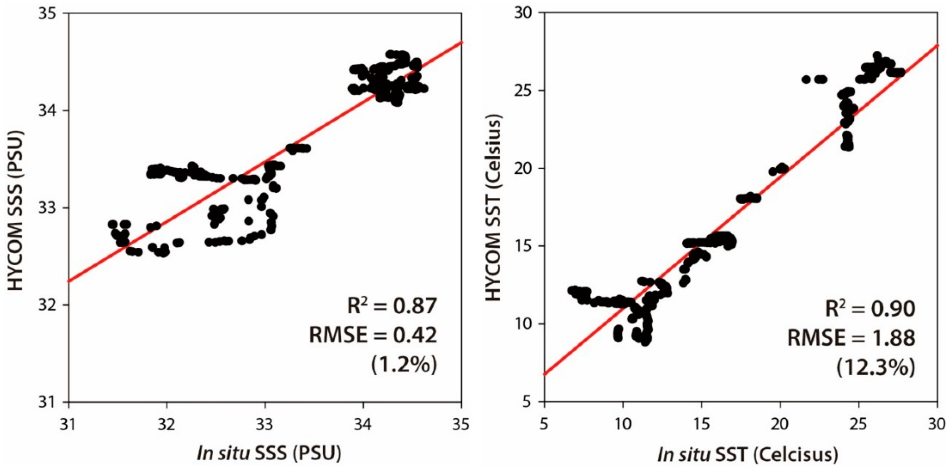
Although the number of in situ measurements used in this study was relatively small, they cover spring (March, April, and May), summer (August), and fall (October and November), which implies that the proposed models can be used to estimate surface seawater ƒCO2 in any season except winter. In case of SST and SSS, the difference between in situ measurements and HYCOM data might increase the uncertainty of the models, although the relationships between the two are moderately good with R2 ~ 0.87–0.9 (Figure 3). It should be noted that HYCOM data are daily while in situ data are time-specific (between 9 a.m. and 4 p.m.) and thus some discrepancies between the two exist. In addition, the discrepancies occur due to the different spatial scale: while the spatial resolution of HYCOM is 1/8 degrees, in situ samples are point-based. Thus, when multiple in situ samples were located in a grid of HYCOM, they were averaged. Since there were no in situ Chl-a and CDOM data, it was not possible to compare them to satellite-derived products.
SVR is known to be suitable for modeling especially when the training sample size is small [64,65,66,67], it was right in this study. As the selection and optimization of a kernel function is critical for successful modeling in SVR, the use of different kernel functions and parameters might improve the performance. RF uses an ensemble approach (i.e., numerous trees), which is efficient at modeling the nonlinear characteristics of surface seawater ƒCO2. By using 500 independent trees, a well-known overfitting problem when using a single tree was effectively mitigated in this study [57]. RF showed the highest accuracy in this study. Both linear and nonlinear characteristics of surface seawater ƒCO2 were effectively modeled using the RF approach. Since RF uses an ensemble approach (i.e., combining numerous independent tree results), it appeared to be less sensitive to overfitting, resulting in higher validation accuracy, when compared to the other approaches. More training samples can mitigate validation accuracy of the two machine learning approaches in further study.
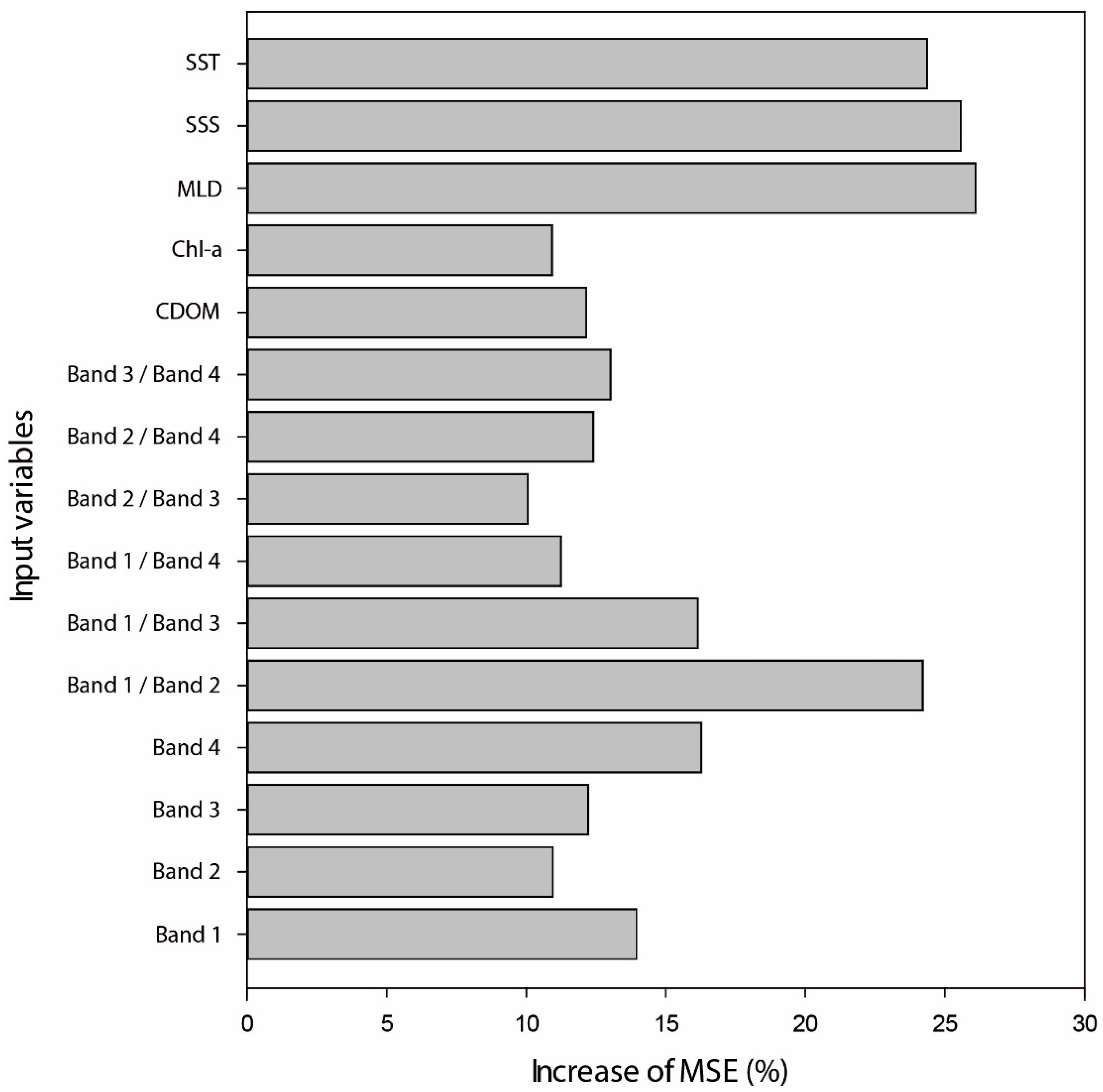
Figure 4 summarizes the relative variable importance provided by RF. From the variable importance identified by RF, the three ocean parameters (i.e., SST, SSS, and MLD) were considered more important than the individual band reflectance data, except for the ratio between bands 1 and 2. Although some of the ocean parameters were generated using satellite band reflectance data, it appears that the band reflectance data only by themselves were not able to effectively model surface seawater ƒCO2 without other input variables using the three machine learning approaches. MLD was identified as the most important variable for RF models. MLD is the second least correlated to surface seawater ƒCO2 (Table 5), but becomes the most important variable in the RF model, which implies that there is a nonlinear relationship between MLD and surface seawater ƒCO2. While MLD and ƒCO2 showed a relatively positive relationship in the spring season, no clear pattern (but with some clusters) was found in the summer and autumn seasons (not shown). This nonlinear seasonality with clusters could be well addressed by the rules produced in RF. Since MLD is a result of vertical mixing, it is a parameter controlling surface seawater ƒCO2 [23]. By controlling stratification and subsequent vertical mixing, salinity influences to ƒCO2. As SST is related to solubility of CO2, and directly affects biological processes [7], it has been commonly used to estimate the partial pressure of CO2 [10,11,14,17]. The various carbon pumps in the ocean carbon cycle are directly or indirectly related to SST.
Among band reflectance data, band 4 and the ratio between bands 1 and 2 were identified as important in an RF model. The ratio between bands 3 and 4 is used to make CDOM and Chl-a products and band 2 is used to make CDOM for GOCI [76]. Results from the RF model showed that there are several other bands and band ratios that are important to estimate surface seawater ƒCO2, which are not used to make ocean parameters for GOCI. This implies that only using a few ocean parameters for predicting surface seawater ƒCO2 might not be ideal because they do not represent all major biological processes occurring in surface seawater with different environments. In that regard, individual band reflectance data can be used as good supplements for modeling ƒCO2.
4.2. Spatial and Temporal Distribution of Surface Seawater ƒCO2
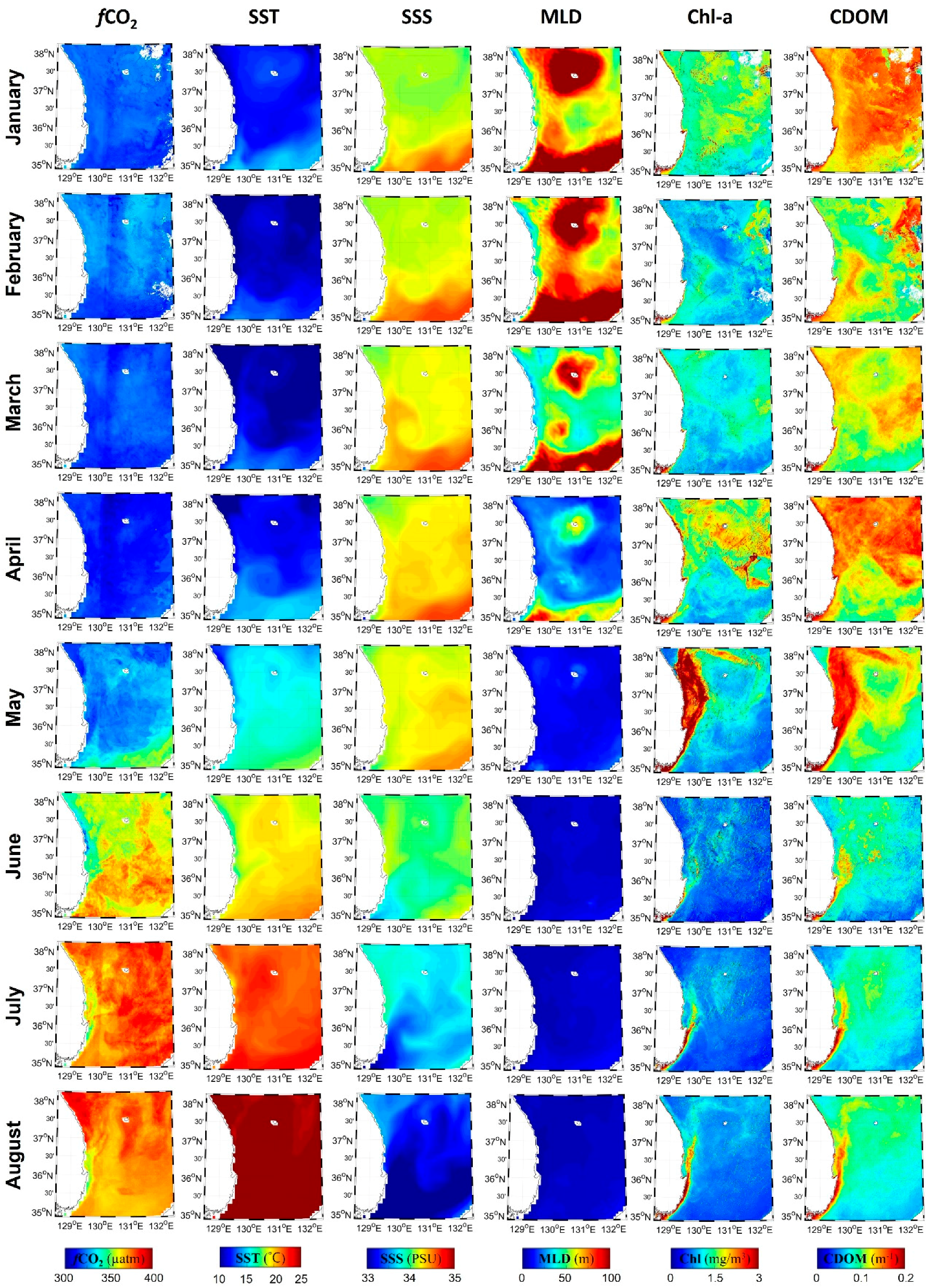
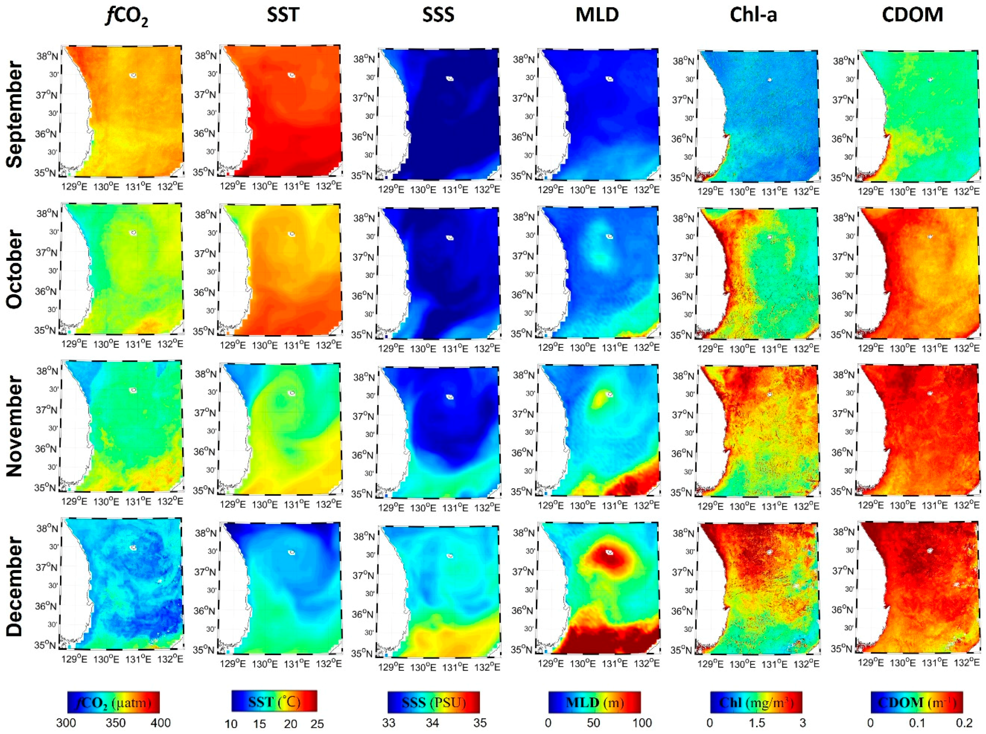
We applied the RF model, which produced the best performance, to GOCI satellite and HYCOM reanalysis images, and examined the seasonal variability of surface seawater ƒCO2 averaged by month in 2015. The GOCI images collected around 1:30 p.m. were used to produce the distribution of surface seawater ƒCO2. Satellite-based surface seawater ƒCO2 maps show similar spatial distribution with in situ measurements (Figure 1). The spatial distribution of GOCI-estimated surface seawater ƒCO2 has a similar pattern to those of SST, SSS, and MLD (Figure 5), which are highly affected by ocean currents in the East Sea [77]. While the estimated surface seawater ƒCO2 generally shows a similar monthly pattern with SSS and SST, it is substantially influenced by MLD when MLD shows extreme variations. The estimated monthly surface seawater ƒCO2 in summer (June, July, and August) might be affected by an inflow of warm current from the south, and it shows similar distribution to HYCOM SSS and SST. The low surface seawater ƒCO2 in coastal areas in July, August, and September appears to be related to biological activity, which implies that high biological activities reduce surface seawater ƒCO2 values. This agrees with in situ measurements in August showing low surface seawater ƒCO2 values in coastal regions (Figure 1). The vortex pattern of the estimated surface seawater ƒCO2 in fall is derived by the distributions of ocean parameters of MLD, SSS, SST, and Chl-a (Figure 5). Especially, patches with relatively high ƒCO2 values found in the southern part of the East Sea in June are mainly associated with lower SSS values.
Many factors are related with the uncertainty of the spatial distribution of ƒCO2 produced from the proposed approach. First of all, input parameters, especially ocean parameters from GOCI and HYCOM, contain their own uncertainties, which are inherent in the distribution of ƒCO2. This implies that more robust and reliable products of ocean parameters may further reduce the uncertainty of estimated ƒCO2. For example, the operational algorithms of GOCI standard products (e.g., chl-a and CDOM) will be upgraded in the GOCI Data Processing System (GDPS) and available later in 2017, which implies that the accuracy of ƒCO2 estimation may improve with the new products in the future. In addition, it should be noted that the different numbers of daily ƒCO2 data by pixel were used to generate the spatial distribution of ƒCO2 for each month mainly due to cloud cover. In particular, the areas with high environmental changes in terms of currents and biological activities appeared to have relatively high uncertainty of the spatial distribution of ƒCO2.
Compared to in situ measurement data, the estimated surface seawater ƒCO2 in November show lower values. This is likely due to temporal bias of in situ measurements that covered only one day (15 November). The surface seawater ƒCO2 values in summer are higher than other seasons mainly due to higher SST values. An increase in SST raises surface seawater ƒCO2 thermodynamically [38]. Biological activity controlling surface seawater ƒCO2 is also lowest in summer except coastal areas due to lack of nutrients. Surface seawater ƒCO2 values in fall and winter are higher than those in spring, and variations in biological production, SST, and MLD can explain these seasonal differences [20]. Deeper MLD in winter brings subsurface waters with high CO2 concentrations to the surface, leading to higher surface seawater ƒCO2 values. Nutrients supplied from subsurface to the surface by deepening of MLD cause an increase of biological production in the following spring, resulting in a decrease of ƒCO2 values. In addition to higher biological production, lower SST values in spring compared to those in fall are also responsible for lower surface seawater ƒCO2 values in spring. Seasonal variations of estimated ƒCO2 values correspond well to measured seasonal changes in surface seawater ƒCO2 in the East Sea [78]. Since the in situ data are a bit limited, only covering spring, summer, and fall, there might be high uncertainty of ƒCO2 estimation during the winter season.
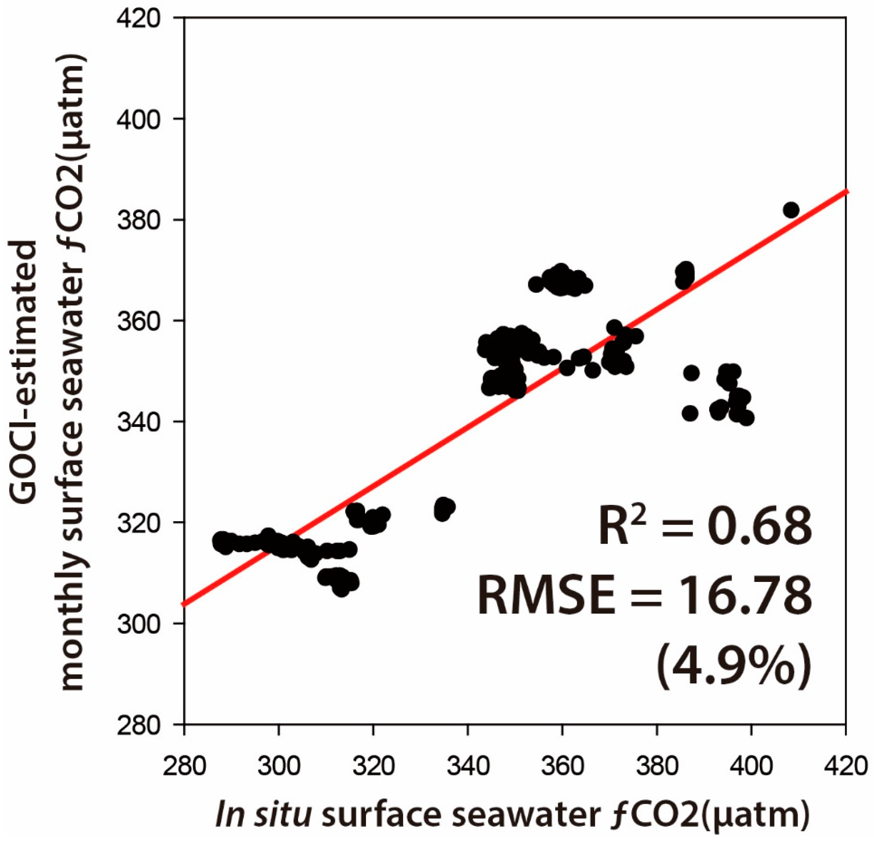
Validation of the monthly distribution of ƒCO2 produced from GOCI and HYCOM data was conducted using the in situ measurements. In situ ƒCO2 measurements collected around the time of data collection of GOCI (collection time is around 1:30 p.m.) were averaged by month and compared with the monthly surface seawater ƒCO2 estimation from GOCI and HYCOM data in each pixel (Figure 6). It should be noted, though, that there is a temporal discrepancy between the two: while the daily satellite-estimated ƒCO2 images were averaged for cloud-free days over a month, in situ measurements for only a few days per month were averaged for comparison. Nonetheless, the results are very promising, which supports the use of machine learning and satellite data fusion approaches for the estimation of surface seawater ƒCO2.
4.3. Sea-Air CO2 Fluxes
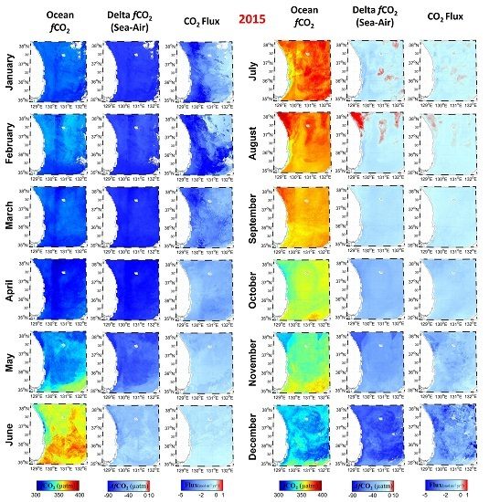
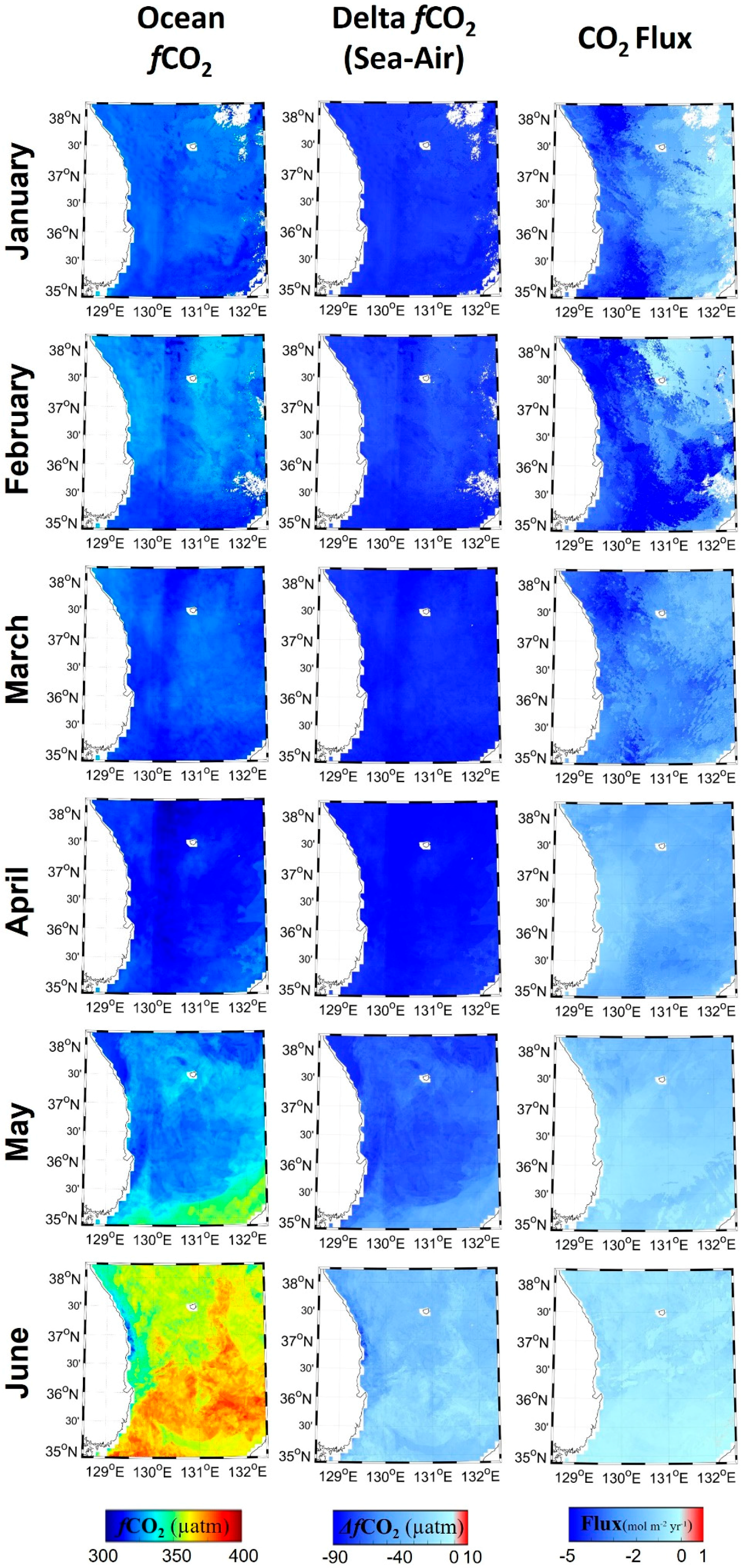
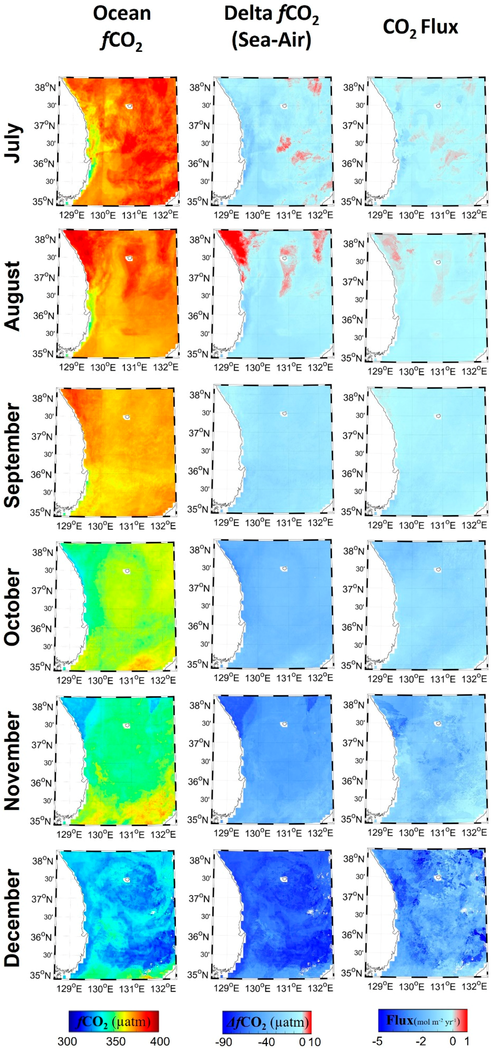
Figure 7 is monthly distributions of surface seawater ƒCO2, delta (sea-air) ƒCO2, and sea-air CO2 flux for the reference year 2015 calculated using Equation (3), and Table 6 shows monthly mean values of each factor in the whole study area (the East Sea) in 2015. The spatial distributions of delta (sea-air) ƒCO2 and sea-air CO2 flux have similar patterns to those of predicted surface seawater ƒCO2 and SST (Figure 5). In the case of delta (sea-air) ƒCO2 and sea-air CO2 flux, the blue color depicts absorption of carbon from the atmosphere (negative value; carbon sink) and red color depicts efflux of carbon (positive value; carbon source) from the ocean. Seasonal changes of CO2 flux between the ocean and atmosphere clearly appeared in Figure 7. Overall, the East Sea absorbs CO2 from the atmosphere throughout the whole region, acts as a sink for atmospheric CO2, except some areas in July and August (Figure 7 and Table 6). Monthly mean delta (sea-air) ƒCO2 shows a minimum in April and a maximum in August that is in agreement with the result of [20] (Table 6). The largest CO2 flux to the ocean was estimated in winter and the lowest flux was found in summer. The annual mean CO2 flux value of −1.53 mol m−2 year−1 estimated in this study is slightly lower than the value of CO2 flux (−2.47 ± 1.26 mol m−2 year−1) reported in the Ulleung Basin of the East Sea [78]. This is due to fact that the Ulleung Basin is the most productive area in the East Sea except coastal regions, and our study area is much larger than that of [78].
The amount of absorbed CO2 was smaller from June to September than the other months (Delta ƒCO2 from June to September ranged from −29.50 to −4.14 µatm while the yearly mean was −48.92 µatm; CO2 flux from June to September ranged from −0.56 to −0.11 mol m−2 year−1 while the yearly mean was −1.53 mol m−2 year−1). This lower uptake of atmospheric CO2 in summertime is mainly due to higher SST than the other seasons. Increase of SST causes a decrease of solubility, leading to an increase of surface seawater ƒCO2. Lower biological production compared to other seasons also resulted in higher surface seawater ƒCO2 and less negative or positive delta (sea-air) ƒCO2 values. While the highest monthly mean surface seawater ƒCO2 value was observed in July, the highest monthly mean delta (sea-air) ƒCO2 (−4.14 µatm) and the lowest monthly mean CO2 flux to the ocean (−0.11 mol m−2 year−1) was shown in August (Table 6). This is due to lower atmospheric CO2 values in August than in July. The seasonal cycle of atmospheric CO2 is in the opposite phase to that of surface seawater ƒCO2 according to the intensity of land biosphere production. In addition, the month with the lowest monthly mean delta (sea-air) ƒCO2 (April) does not correspond to that with the highest monthly mean CO2 flux to the ocean (February) due to higher wind speed in winter compared to in spring. Variation of wind speed has a significant impact on the changes in sea-air CO2 fluxes (see Equation (3)). For the period from July to August, some areas of the East Sea experienced weakly positive CO2 fluxes (red color) implying a release of CO2 to the atmosphere. The areas showing positive flux values in August correspond well to those with relatively higher SSS values (Figure 5), leading to higher surface seawater ƒCO2 by decreasing solubility.
5. Conclusions
This study estimated the surface seawater ƒCO2 in the East Sea of Korea using in situ measurements, GOCI satellite and their derived products, and HYCOM reanalysis data through MNR and two machine learning approaches (RF and SVR). Results show that RF generally produced a better performance than MNR and SVR. RF effectively modeled both linear and nonlinear characteristics of surface seawater ƒCO2 through an ensemble approach. Ocean parameters (i.e., SSS, SST, and MLD) appeared to be more contributing than the individual bands or band ratios from the satellite data. Since MLD controls the amount of carbon dioxide moving into the surface from the subsurface, it may be very useful for estimating surface seawater ƒCO2. It should be noted, however, that HYCOM MLD uses a fixed threshold of change in the vertical profile of temperature to identify the depth.
The monthly surface seawater ƒCO2 maps in 2015 provided valuable information of seasonal spatial variations of surface seawater ƒCO2 in the East Sea. Strong saturations of CO2 in the ocean was observed in summer because of increased SST. Surface seawater ƒCO2 was higher in fall than spring because of a higher SST and deeper MLD [20]. The spatial distribution of surface seawater ƒCO2 in the East Sea showed a strong link with SST, SSS, and MLD in GOCI-based estimation. Overall, the East Sea is a sink for atmospheric CO2, although some areas in summer act as a weak CO2 source.
Compared to the existing literature that used traditional regression models [8,10,11,12,16,17,19], this study estimated surface seawater ƒCO2 with complicated, but more advanced algorithms than conventional statistical ones, using two machine learning approaches. In addition, using the world first geostationary ocean color satellite data (i.e., GOCI), we were able to improve the model performance: much more data collection by GOCI allowed us to use more samples temporally matched between in situ measurements and satellite-derived data. However, there are several limitations of this study, for which further research is needed. In situ measurements data used in this study only cover a few months in spring, summer, and fall. Longer time series data should be investigated to make the model much more robust and reliable. Uncertainty of satellite-derived products should also be reduced, especially near the coastal areas.
Acknowledgments
This research was supported by “Development of satellite based ocean carbon flux model for seas around Korea” funded by the Ministry of Ocean and Fisheries, Republic of Korea, and Technology Development Program to Solve Climate Changes through the National Foundation of Korea (NRF) funded by the Ministry of Science, ICT, and Future Planning of Korea (Grant: NRF-2012M1A2A2671851).
Author Contributions
Eunna Jang led manuscript writing and contributed to the data analysis and research design. Jungho Im supervised this study, contributed to the research design and manuscript writing, and served as the corresponding author. Geun-Ha Park and Young-Gyu Park contributed to the discussion of the results and manuscript writing.
Conflicts of Interest
The authors declare no conflict of interest.
References
- Pachauri, R.K.; Allen, M.R.; Barros, V.R.; Broome, J.; Cramer, W.; Christ, R.; Church, J.A.; Clarke, L.; Dahe, Q.; Dasgupta, P.; et al. Climate Change 2014: Synthesis Report. Contribution of Working Groups I, II and III to the Fifth Assessment Report of the Intergovernmental Panel on Climate Change; Pachauri, R., Meyer, L., Eds.; IPCC: Geneva, Switzerland, 2014. [Google Scholar]
- Sabine, C.L.; Feely, R.A.; Gruber, N.; Key, R.M.; Lee, K.; Bullister, J.L.; Wanninkhof, R.; Wong, C.; Wallace, D.W.; Tilbrook, B. The oceanic sink for anthropogenic CO2. Science 2004, 305, 367–371. [Google Scholar] [CrossRef] [PubMed] [Green Version]
- Takahashi, T.; Sutherland, S.C.; Wanninkhof, R.; Sweeney, C.; Feely, R.A.; Chipman, D.W.; Hales, B.; Friederich, G.; Chavez, F.; Sabine, C. Climatological mean and decadal change in surface ocean pCO2, and net sea–air CO2 flux over the global oceans. Deep Sea Res. Part II Top. Stud. Oceanogr. 2009, 56, 554–577. [Google Scholar] [CrossRef] [Green Version]
- Raven, J.; Caldeira, K.; Elderfield, H.; Hoegh-Guldberg, O.; Liss, P.; Riebesell, U.; Shepherd, J.; Turley, C.; Watson, A. Ocean Acidification Due to Increasing Atmospheric Carbon Dioxide; The Royal Society: London, UK, 2005. [Google Scholar]
- Sung, C.-G.; Kim, T.W.; Park, Y.-G.; Kang, S.-G.; Inaba, K.; Shiba, K.; Choi, T.S.; Moon, S.-D.; Litvin, S.; Lee, K.-T. Species and gamete-specific fertilization success of two sea urchins under near future levels of pCO2. J. Mar. Syst. 2014, 137, 67–73. [Google Scholar] [CrossRef]
- Zeng, J.; Nojiri, Y.; Landschützer, P.; Telszewski, M.; Nakaoka, S. A global surface ocean ƒCO2 climatology based on a feed-forward neural network. J. Atmos. Ocean. Technol. 2014, 31, 1838–1849. [Google Scholar] [CrossRef]
- Bai, Y.; Cai, W.J.; He, X.; Zhai, W.; Pan, D.; Dai, M.; Yu, P. A mechanistic semi-analytical method for remotely sensing sea surface pCO2 in river-dominated coastal oceans: A case study from the East China Sea. J. Geophys. Res. Oceans 2015, 120, 2331–2349. [Google Scholar] [CrossRef]
- Borges, A.V.; Ruddick, K.; Lacroix, G.; Nechad, B.; Asteroca, R.; Rousseau, V.; Harlay, J. Estimating pCO2 from Remote Sensing in the Belgian Coastal Zone. Available online: http://orbi.ulg.be/bitstream/2268/81111/1/borges_et_al_2010_esa_living_planet%5B1%5D.pdf (accessed on 10 August 2017).
- Chen, S.; Hu, C.; Byrne, R.H.; Robbins, L.L.; Yang, B. Remote estimation of surface pCO2 on the West Florida Shelf. Cont. Shelf Res. 2016, 128, 10–25. [Google Scholar] [CrossRef]
- Chierici, M.; Olsen, A.; Johannessen, T.; Trinañes, J.; Wanninkhof, R. Algorithms to estimate the carbon dioxide uptake in the northern North Atlantic using shipboard observations, satellite and ocean analysis data. Deep Sea Res. Part II Top. Stud. Oceanogr. 2009, 56, 630–639. [Google Scholar] [CrossRef]
- Chierici, M.; Signorini, S.R.; Fransson, A.; Olsen, A. Surface water ƒCO2 algorithms for the high-latitude Pacific sector of the Southern Ocean. Remote Sens. Environ. 2012, 119, 184–196. [Google Scholar] [CrossRef]
- Cosca, C.E.; Feely, R.A.; Boutin, J.; Etcheto, J.; McPhaden, M.J.; Chavez, F.P.; Strutton, P.G. Seasonal and interannual CO2 fluxes for the central and eastern equatorial Pacific Ocean as determined from ƒCO2-SST relationships. J. Geophys. Res. Oceans 2003, 108. [Google Scholar] [CrossRef]
- Hales, B.; Strutton, P.G.; Saraceno, M.; Letelier, R.; Takahashi, T.; Feely, R.; Sabine, C.; Chavez, F. Satellite-Based prediction of pCO2 in coastal waters of the eastern North Pacific. Prog. Oceanogr. 2012, 103, 1–15. [Google Scholar] [CrossRef]
- Jo, Y.H.; Dai, M.; Zhai, W.; Yan, X.H.; Shang, S. On the variations of sea surface pCO2 in the northern South China Sea: A remote sensing based neural network approach. J. Geophys. Res Oceans 2012, 117. [Google Scholar] [CrossRef]
- Landschützer, P.; Gruber, N.; Bakker, D.; Schuster, U.; Nakaoka, S.; Payne, M.; Sasse, T.; Zeng, J. A neural network-based estimate of the seasonal to inter-annual variability of the Atlantic Ocean carbon sink. Biogeosciences 2013, 10, 7793–7815. [Google Scholar] [CrossRef] [Green Version]
- Lauvset, S.K.; Chierici, M.; Counillon, F.; Omar, A.; Nondal, G.; Johannessen, T.; Olsen, A. Annual and seasonal ƒCO2 and air–sea CO2 fluxes in the Barents Sea. J. Mar. Syst. 2013, 113, 62–74. [Google Scholar] [CrossRef]
- Ono, T.; Saino, T.; Kurita, N.; Sasaki, K. Basin-Scale extrapolation of shipboard pCO2 data by using satellite SST and Chl-a. Int. J. Remote Sens. 2004, 25, 3803–3815. [Google Scholar] [CrossRef]
- Sarma, V.; Saino, T.; Sasaoka, K.; Nojiri, Y.; Ono, T.; Ishii, M.; Inoue, H.; Matsumoto, K. Basin-Scale pCO2 distribution using satellite sea surface temperature, Chl-a, and climatological salinity in the North Pacific in spring and summer. Glob. Biogeochem. Cycles 2006, 20. [Google Scholar] [CrossRef]
- Tao, Z.; Qin, B.; Li, Z.; Yang, X. Satellite observations of the partial pressure of carbon dioxide in the surface water of the Huanghai Sea and the Bohai Sea. Acta Oceanol. Sin. 2012, 31, 67–73. [Google Scholar] [CrossRef]
- Kim, J.Y.; Kang, D.J.; Lee, T.; Kim, K.R. Long-Term trend of CO2 and ocean acidification in the surface water of the Ulleung Basin, the East/Japan sea inferred from the underway observational data. Biogeosciences 2014, 11, 2443. [Google Scholar] [CrossRef] [Green Version]
- Else, B.G.; Yackel, J.J.; Papakyriakou, T.N. Application of satellite remote sensing techniques for estimating air–sea CO2 fluxes in Hudson Bay, Canada during the ice-free season. Remote Sens. Environ. 2008, 112, 3550–3562. [Google Scholar] [CrossRef]
- Telszewski, M.; Chazottes, A.; Schuster, U.; Watson, A.; Moulin, C.; Bakker, D.; González-Dávila, M.; Johannessen, T.; Körtzinger, A.; Luger, H.O. Estimating the monthly pCO2 distribution in the north Atlantic using a self-organizing neural network. Biogeosciences 2009, 6, 1405–1421. [Google Scholar] [CrossRef] [Green Version]
- Park, G.H.; Lee, K.; Tishchenko, P.; Min, D.H.; Warner, M.J.; Talley, L.D.; Kang, D.J.; Kim, K.R. Large accumulation of anthropogenic CO2 in the East (Japan) Sea and its significant impact on carbonate chemistry. Glob. Biogeochem. Cycles 2006, 20. [Google Scholar] [CrossRef]
- Park, Y.G.; Choi, S.H.; Kim, C.H. Assessment of pCO2 in the Yellow and East China Sea using an earth system model. Ocean Polar Res. 2011, 33, 447–455. [Google Scholar] [CrossRef]
- Gamo, T.; Momoshima, N.; Tolmachyov, S. Recent upward shift of the deep convection system in the Japan Sea, as inferred from the geochemical tracers tritium, oxygen, and nutrients. Geophys. Res. Lett. 2001, 28, 4143–4146. [Google Scholar] [CrossRef]
- Kim, K.; Kim, K.R.; Min, D.H.; Volkov, Y.; Yoon, J.H.; Takematsu, M. Warming and structural changes in the East (Japan) Sea: A clue to future changes in global Oceans? Geophys. Res. Lett. 2001, 28, 3293–3296. [Google Scholar] [CrossRef]
- Min, D.H.; Warner, M.J. Basin-Wide circulation and ventilation study in the East Sea (Sea of Japan) using chlorofluorocarbon tracers. Deep Sea Res. Part II Top. Stud. Oceanogr. 2005, 52, 1580–1616. [Google Scholar] [CrossRef]
- Park, Y.G.; Park, J.H.; Lee, H.J.; Min, H.S.; Kim, S.D. The effects of geothermal heating on the East/Japan sea circulation. J. Geophys. Res. Oceans 2013, 118, 1893–1905. [Google Scholar] [CrossRef]
- Park, Y.G. The effects of Tsushima warm current on the interdecadal variability of the East/Japan Sea thermohaline circulation. Geophys. Res. Lett. 2007, 34. [Google Scholar] [CrossRef]
- Choi, S.H.; Kim, D.; Shim, J.; Min, H.S. The spatial distribution of surface ƒCO2 in the Southwestern East Sea/Japan Sea during summer 2005. Ocean Sci. J. 2011, 46, 13. [Google Scholar] [CrossRef]
- Park, Y.G.; Seol, K.H.; Boo, K.O.; Lee, J.; Cho, C.; Byun, Y.H.; Seo, S. Acidification at the surface in the marginal seas around Korea: A coupled climate-carbon cycle model study. 2017; under review. [Google Scholar]
- Park, S.; Lee, T.; Jo, Y.H. Sea surface pCO2 and its variability in the Ulleung Basin, East Sea constrained by a neural network model. Sea 2016, 21, 1–10. [Google Scholar] [CrossRef]
- Chen, F.; Cai, W.J.; Benitez-Nelson, C.; Wang, Y. Sea surface pCO2-SST relationships across a cold-core cyclonic eddy: Implications for understanding regional variability and air-sea gas exchange. Geophys. Res. Lett. 2007, 34. [Google Scholar] [CrossRef]
- Parard, G.; Charantonis, A.A.; Rutgerson, A. Remote sensing the sea surface CO2 of the Baltic Sea using the SOMLO methodology. Biogeosciences 2015, 12, 3369–3384. [Google Scholar] [CrossRef]
- Parard, G.; Charantonis, A.A.; Rutgersson, A. Using satellite data to estimate partial pressure of CO2 in the Baltic Sea. J. Geophys. Res. Biogeosci. 2016, 121, 1002–1015. [Google Scholar] [CrossRef]
- Dickson, A.G.; Sabine, C.L.; Christian, J.R. Guide to Best Practices for Ocean CO2 Measurements; North Pacific Marine Science Organization: Sidney, BC, Canada, 2007; p. 191. [Google Scholar]
- Pierrot, D.; Neill, C.; Sullivan, K.; Castle, R.; Wanninkhof, R.; Lüger, H.; Johannessen, T.; Olsen, A.; Feely, R.A.; Cosca, C.E. Recommendations for autonomous underway pCO2 measuring systems and data-reduction routines. Deep Sea Res. Part II Top. Stud. Oceanogr. 2009, 56, 512–522. [Google Scholar] [CrossRef]
- Millero, F.J. Thermodynamics of the carbon dioxide system in the Oceans. Geochim. Cosmochim. Acta 1995, 59, 661–677. [Google Scholar] [CrossRef]
- Korea Ocean Satellite Center (KOSC) Website. Available online: http://kosc.kiost.ac.kr/eng/ (accessed on 3 March 2016).
- KOSC Website. Available online: http://kosc.kiost.ac/ (accessed on 3 March 2016).
- HYCOM + NCODA Homepage. Available online: http://tds.hycom.org/thredds/catalog.html (accessed on 3 March 2016).
- Dlugokency, E.J.; Masarie, K.A.; Lang, P.M.; Tans, P.P. NOAA Greenhouse Gas Reference from Atmospheric Carbon Dioxide Dry Air Mole Fractions from the NOAA ESRL Carbon Cycle Cooperative Global Air Sampling Network. Available online: ftp://aftp.cmdl.noaa.gov/data/trace_gases/co2/flask/surface/ (accessed on 10 October 2016).
- NOAA ESRL Greenhouse Gas MBL Reference Homepage. Available online: https://www.esrl.noaa.gov/gmd/ccgg/mbl/mbl.html (accessed on 3 March 2016).
- Berrisford, P.; Dee, D.; Poli, P.; Brugge, R.; Fielding, K.; Fuentes, M.; Kallberg, P.; Kobayashi, S.; Uppala, S.; Simmons, A. The ERA-Interim Archive Version 2.0; ERA Report Series 1; ECMWF: Reading, UK, 2011. [Google Scholar]
- ECMWF Homepage. Available online: http://apps.ecmwf.int/datasets/data/interim-full-daily/levtype=sfc/ (accessed on 3 March 2016).
- Breiman, L. Random forests. Mach. Learn. 2001, 45, 5–32. [Google Scholar] [CrossRef]
- Jensen, J.R.; Im, J. Remote sensing change detection in urban environments. In Geo-Spatial Technologies in Urban Environments; Springer: Berlin/Heidelberg, Germany, 2007; pp. 7–31. [Google Scholar]
- Im, J.; Jensen, J.R.; Coleman, M.; Nelson, E. Hyperspectral remote sensing analysis of short rotation woody crops grown with controlled nutrient and irrigation treatments. Geocarto Int. 2009, 24, 293–312. [Google Scholar] [CrossRef]
- Lu, Z.; Im, J.; Quackenbush, L.J. A volumetric approach to population estimation using LiDAR remote sensing. Photogramm. Eng. Remote Sens. 2011, 77, 1145–1156. [Google Scholar] [CrossRef]
- Rhee, J.; Im, J.; Carbone, G.J.; Jensen, J.R. Delineation of climate regions using in-situ and remotely sensed data for the Carolinas. Remote Sens. Environ. 2008, 112, 3099–3111. [Google Scholar] [CrossRef]
- Richardson, H.J.; Hill, D.J.; Denesiuk, D.R.; Fraser, L.H. A comparison of geographic datasets and field measurements to model soil carbon using Random Forests and stepwise regressions (British Columbia, Canada). GISci. Remote Sens. 2017, 54, 573–591. [Google Scholar] [CrossRef]
- Rhee, J.; Im, J. Meteorological drought forecasting for ungauged areas based on machine learning: Using long-range climate forecast and remote sensing data. Agric. For. Meteorol. 2017, 237, 105–122. [Google Scholar] [CrossRef]
- Park, S.; Im, J.; Park, S.; Rhee, J. Drought monitoring using high resolution soil moisture through multi-sensor satellite data fusion over the Korean peninsula. Agric. For. Meteorol. 2017, 237, 257–269. [Google Scholar] [CrossRef]
- Lee, S.; Im, J.; Kim, J.; Kim, M.; Shin, M.; Kim, H.-C.; Quackenbush, L.J. Arctic sea ice thickness estimation from Cryosat-2 satellite data using machine learning-based lead detection. Remote Sens. 2016, 8, 698. [Google Scholar] [CrossRef]
- Lee, S.; Han, H.; Im, J.; Jang, E.; Lee, M.-I. Detection of deterministic and probabilistic convection initiation using Himawari-8 advanced Himawari imager data. Atmos. Meas. Tech. 2017, 10, 1859. [Google Scholar] [CrossRef]
- Lu, Z.; Im, J.; Rhee, J.; Hodgson, M. Building type classification using spatial and landscape attributes derived from LiDAR remote sensing data. Landsc. Urban Plan. 2014, 130, 134–148. [Google Scholar] [CrossRef]
- Belgiu, M.; Drăgut, L. Random forest in remote sensing: A review of applications and future directions. ISPRS J. Photogramm. Remote Sens. 2016, 114, 24–31. [Google Scholar] [CrossRef]
- Kim, Y.H.; Im, J.; Ha, H.K.; Choi, J.K.; Ha, S. Machine learning approaches to coastal water quality monitoring using GOCI satellite data. GISci. Remote Sens. 2014, 51, 158–174. [Google Scholar] [CrossRef]
- Kim, M.; Im, J.; Han, H.; Kim, J.; Lee, S.; Shin, M.; Kim, H.C. Landfast sea ice monitoring using multisensor fusion in the Antarctic. GISci. Remote Sens. 2015, 52, 239–256. [Google Scholar] [CrossRef]
- Pal, M. Random forest classifier for remote sensing classification. Int. J. Remote Sens. 2005, 26, 217–222. [Google Scholar] [CrossRef]
- Rhee, J.; Park, S.; Lu, Z. Relationship between land cover patterns and surface temperature in urban areas. GISci. Remote Sens. 2014, 51, 521–536. [Google Scholar] [CrossRef]
- Torbick, N.; Corbiere, M. Mapping urban sprawl and impervious surfaces in the Northeast United States for the past four decades. GISci. Remote Sens. 2015, 52, 746–764. [Google Scholar] [CrossRef]
- Mountrakis, G.; Im, J.; Ogole, C. Support vector machines in remote sensing: A review. ISPRS J. Photogramm. Remote Sens. 2011, 66, 247–259. [Google Scholar] [CrossRef]
- Foody, G.M.; Mathur, A. The use of small training sets containing mixed pixels for accurate hard image classification: Training on mixed spectral responses for classification by a SVM. Remote Sens. Environ. 2006, 103, 179–189. [Google Scholar] [CrossRef]
- Shin, K.S.; Lee, T.S.; Kim, H.J. An application of support vector machines in bankruptcy prediction model. Expert Syst. Appl. 2005, 28, 127–135. [Google Scholar] [CrossRef]
- Maxwell, A.; Strager, M.; Warner, T.; Zegre, N.; Yuill, C. Comparison of NAIP orthophotography and RapidEye satellite imagery for mapping of mining and mine reclamation. GISci. Remote Sens. 2014, 51, 301–320. [Google Scholar] [CrossRef]
- Moreira, L.C.J.; Teixeira, A.d.S.; Galvão, L.S. Potential of multispectral and hyperspectral data to detect saline-exposed soils in Brazil. GISci. Remote Sens. 2015, 52, 416–436. [Google Scholar] [CrossRef]
- Lin, Z.; Yan, L. A support vector machine classifier based on a new kernel function model for hyperspectral data. GISci. Remote Sens. 2016, 53, 85–101. [Google Scholar] [CrossRef]
- Zeng, J.; Matsunaga, T.; Saigusa, N.; Shirai, T.; Nakaoka, S.-I.; Zheng-Hong, T. Evaluation of three machine learning models for surface ocean CO2 mapping. Ocean Sci. 2017, 13, 303. [Google Scholar] [CrossRef]
- Rao, C.; Malleswara Rao, J.; Senthil Kumar, A.; Lakshmi, B.; Dadhwal, V. Expansion of LISS III swath using AWiFS wider swath data and contourlet coefficients learning. GISci. Remote Sens. 2015, 52, 78–93. [Google Scholar] [CrossRef]
- Xun, L.; Wang, L. An object-based SVM method incorporating optimal segmentation scale estimation using Bhattacharyya Distance for mapping salt cedar (Tamarisk spp.) with QuickBird imagery. GISci. Remote Sens. 2015, 52, 257–273. [Google Scholar] [CrossRef]
- Chang, C.C.; Lin, C.J. LibSVM: A library for support vector machines. ACM Trans. Intell. Syst. Technol. 2011, 2, 27. [Google Scholar] [CrossRef]
- Holt, J.T.; Allen, J.I.; Proctor, R.; Gilbert, F. Error quantification of a high-resolution coupled hydrodynamic–ecosystem coastal–ocean model: Part 1 model overview and assessment of the hydrodynamics. J. Mar. Syst. 2005, 57, 167–188. [Google Scholar] [CrossRef]
- Wanninkhof, R. Relationship between wind speed and gas exchange over the ocean revisited. Limnol. Oceanogr. Methods 2014, 12, 351–362. [Google Scholar] [CrossRef]
- RuleQuest Research. RuleQuest Research Data Mining Tools. 2012. Available online: http://www.rulequest.com/ (accessed on 3 March 2016).
- Moon, J.E.; Park, Y.J.; Ryu, J.H.; Choi, J.K.; Ahn, J.H.; Min, J.E.; Son, Y.B.; Lee, S.J.; Han, H.J.; Ahn, Y.H. Initial validation of GOCI water products against in situ data collected around Korean peninsula for 2010–2011. Ocean Sci. J. 2012, 47, 261–277. [Google Scholar] [CrossRef]
- Lee, K.E. Surface water changes recorded in late quaternary marine sediments of the Ulleung Basin, East Sea (Japan Sea). Palaeogeogr. Palaeoclimatol. Palaeoecol. 2007, 247, 18–31. [Google Scholar] [CrossRef]
- Choi, S.H.; Kim, D.; Shim, J.; Kim, K.H.; Min, H.S.; Kim, K.R. Seasonal variations of surface ƒCO2 and sea-air CO2 fluxes in the Ulleung Basin of the East/Japan. Sea. Terr. Atmos. Ocean. Sci. 2012, 23, 343–353. [Google Scholar] [CrossRef]
Figure 1.
The study area of this research and monthly ƒCO2 distribution based on in situ observations. The red box represents the specific study area in the East Sea where the in situ measurements were conducted.
Figure 1.
The study area of this research and monthly ƒCO2 distribution based on in situ observations. The red box represents the specific study area in the East Sea where the in situ measurements were conducted.
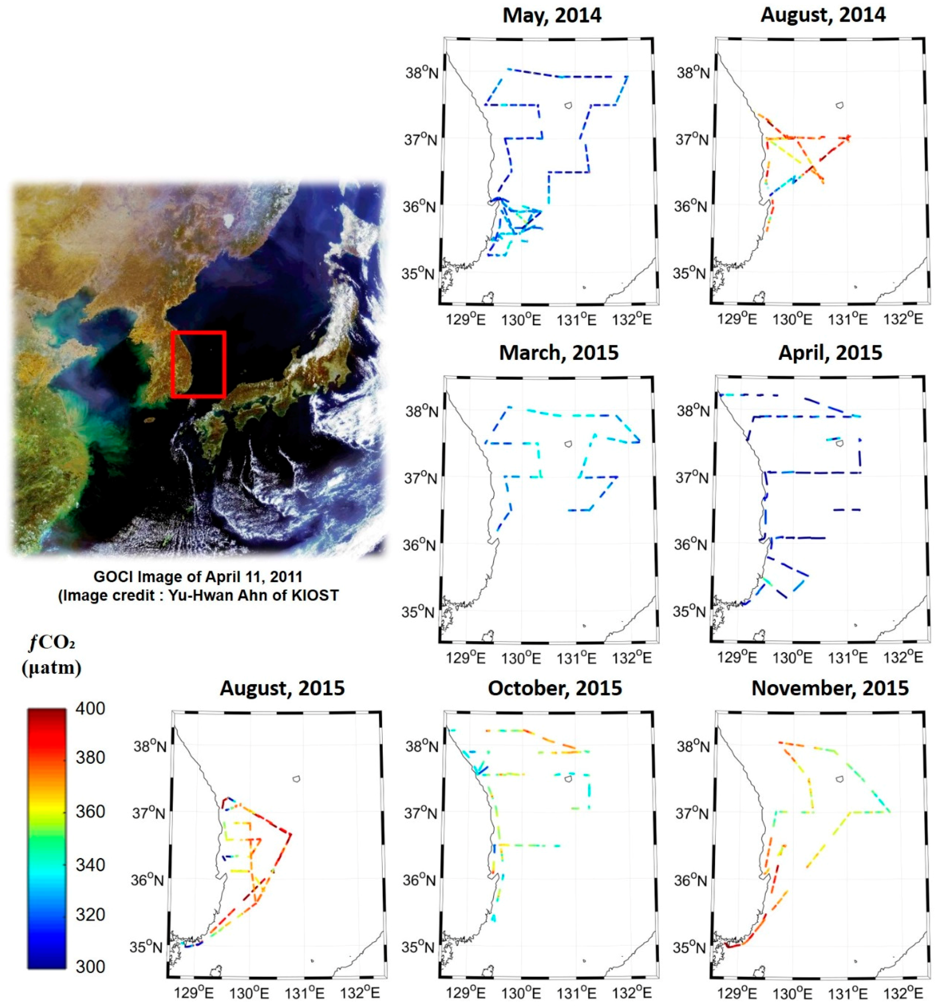
Figure 2.
The result of machine learning-based surface seawater ƒCO2 estimation using (a–d) Geostationary Ocean Color Imater (GOCI) band reflectance data, band ratios, colored dissolved organic matter (CDOM), and chlorophyll-a (Chl-a) and Hybrid Coordinate Ocean Model (HYCOM) mixed layer depth (MLD), sea surface salinity (SSS), and sea surface temperature (SST).
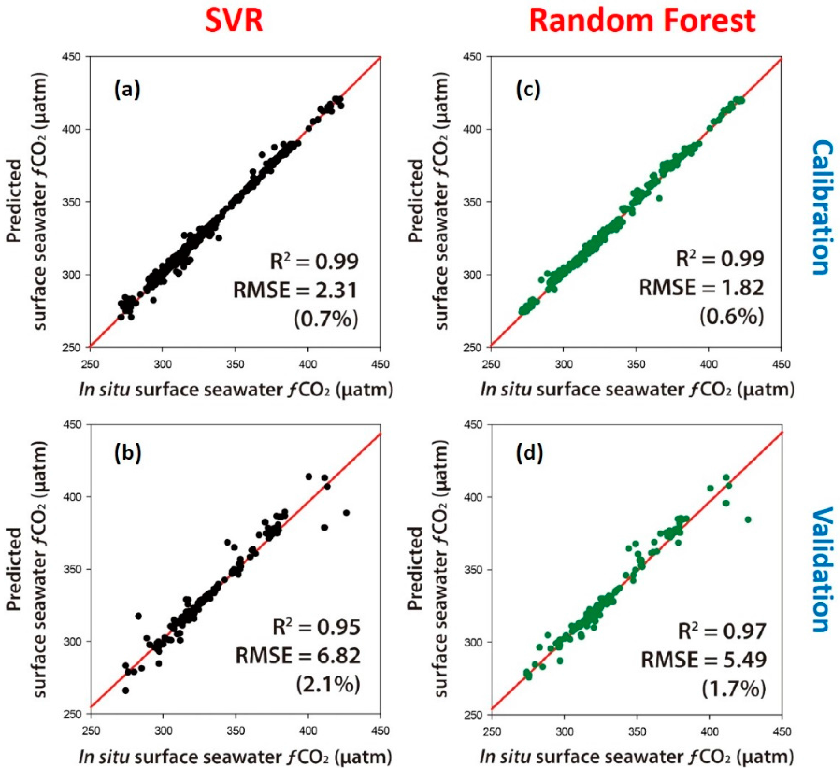
Figure 3.
The comparison of SST and SSS between in situ measurements and HYCOM data.

Figure 4.
Variable importance identified by random forest (RF). Increase of mean squared error (MSE) of RF was calculated using out-of-bag (OOB) data when a variable is perturbed. More explanation about the increase of Mean Square Error (MSE; %) is provided in Section 3.3.1.
Figure 4.
Variable importance identified by random forest (RF). Increase of mean squared error (MSE) of RF was calculated using out-of-bag (OOB) data when a variable is perturbed. More explanation about the increase of Mean Square Error (MSE; %) is provided in Section 3.3.1.

Figure 5.
The monthly surface seawater ƒCO2 produced using the RF model (i.e., GOCI CDOM, Chl-a, and band reflectance data and HYCOM MLD, SSS, and SST), HYCOM SST, SSS, and MLD, and GOCI Chl-a and CDOM distribution maps in 2015. No data pixels in white in the ocean were due to GOCI CDOM and Chl-a data. Please note that Korean Institute of Ocean Science and Technology (KIOST) often provides slot-uncorrected images in L1B band reflectance data, which resulted in an artifact line along longitude 130°E, which is shown in some of the ƒCO2 maps.


Figure 6.
Scatterplots between in situ surface seawater ƒCO2 averaged by month and GOCI-derived monthly ƒCO2.
Figure 6.
Scatterplots between in situ surface seawater ƒCO2 averaged by month and GOCI-derived monthly ƒCO2.

Figure 7.
The surface seawater ƒCO2, delta (sea-air) ƒCO2, and sea-air CO2 flux distribution maps in 2015 for each month.
Figure 7.
The surface seawater ƒCO2, delta (sea-air) ƒCO2, and sea-air CO2 flux distribution maps in 2015 for each month.


Table 1.
Summary of the data used in this study.
| Ship Name (Belong) | In Situ Start Date | In Situ End Date | Latitude | Longitude | In Situ Products | GOCI c Products | HYCOM d Products | Number of In Situ Data Collected in the Ship | Number of Data Matched with Satellite g |
|---|---|---|---|---|---|---|---|---|---|
| Ieodo (KIOST a) | 04/05/2014 07:55 | 11/05/2014 00:25 | 35.24°–36.12°N | 129.38°–130.38°E | Date (YY-MM-DD), Time (hh-mm-dd), Latitude (°), Longitude (°), SST (°C), SSS, Ocean ƒCO2 (μatm) | Chl-a (mg/m3), CDOM (m−1), Band reflectance (Rrs) | SST (°C), SSS MLD (m) | 3348 | 499 |
| Ieodo (KIOST) | 13/05/2014 07:30 | 16/05/2014 10:05 | 35.66°–38.04°N | 129.30°–132.00°E | 1878 | 121 | |||
| Ieodo (KIOST) | 19/08/2014 09:00 | 25/08/2014 11:00 | 35.61°–37.40°N | 129.26°–131.06°E | 3252 | 93 | |||
| Ieodo (KIOST) | 06/03/2015 13:00 | 10/03/2015 07:15 | 36.17°–38.05°N | 129.30°–132.25°E | 1725 | 329 | |||
| Tamgu 3 (NIFS b) e | 08/04/2015 13:00 | 18/04/2015 14:00 | 35.08°–38.22°N | 128.59°–131.27°E | 3193 | 382 | |||
| Ieodo (KIOST) | 10/08/2015 11:55 | 15/08/2015 08:45 | 34.97°–37.22°N | 128.76°–130.77°E | 3226 | 215 | |||
| Tamgu 3 (NIFS) f | 19/10/2015 16:00 | 01/11/2015 10:00 | 35.37°–38.23°N | 128.59°–131.27°E | 2014 | 52 | |||
| Ieodo (KIOST) | 13/11/2015 17:30 | 18/11/2015 07:40 | 34.97°–38.05°N | 128.71°–131.80°E | 2267 | 47 |
KIOST a: Korea Institute of Ocean Science and Technology; NIFS b: National Institute of Fisheries Science; GOCI c: Geostationary Ocean Color Imager; HYCOM d: Hybrid Coordinate Ocean Model; e There are no initial data because of instability of GPS; f There is no latter data because of equipment failure; g The number of data matched with GOCI satellite and HYCOM reanalysis data. The number is different to the number of samples used in machine learning approaches because, when multiple samples fall into one pixel, they were averaged.
Table 2.
Key statistics of in situ surface seawater ƒCO2 measurements (µatm).
| Statistics | May 2014 | August 2014 | March 2015 | April 2015 | August 2015 | October 2015 | November 2015 |
|---|---|---|---|---|---|---|---|
| Maximum | 396.56 | 439.15 | 343.12 | 355.78 | 415.36 | 411.32 | 446.06 |
| Minimum | 287.52 | 297.10 | 306.63 | 252.34 | 226.30 | 317.92 | 336.9 |
| Mean | 323.34 | 374.19 | 327.10 | 304.64 | 373.32 | 351.26 | 369.33 |
| Standard Deviation | 13.21 | 21.91 | 8.97 | 17.09 | 26.11 | 14.85 | 17.25 |
Table 3.
Specification of Geostationary Ocean Color Imager (GOCI) bands used in this study. These four bands were used for input parameters of machine learning approaches.
Table 3.
Specification of Geostationary Ocean Color Imager (GOCI) bands used in this study. These four bands were used for input parameters of machine learning approaches.
| Band | Bandwidth (nm) |
|---|---|
| Band 1 | 402–422 |
| Band 2 | 433–453 |
| Band 3 | 480–500 |
| Band 4 | 545–565 |
Table 4.
Correlation coefficients between input parameters and in situ surface seawater ƒCO2.
| Variables | Correlation Coefficients |
|---|---|
| CDOM a | −0.2082 |
| Chl b | −0.1200 |
| MLD c | −0.0866 |
| SSS d | −0.7335 |
| SST e | 0.7488 |
| Band 1 | 0.2824 |
| Band 2 | 0.2285 |
| Band 3 | 0.1403 |
| Band 4 | −0.0435 |
| Band 1/2 | 0.0627 |
| Band 1/3 | 0.2829 |
| Band 1/4 | 0.2713 |
| Band 2/3 | 0.1810 |
| Band 2/4 | 0.2585 |
| Band 3/4 | 0.1612 |
a colored dissolved organic matter; b chlorophyll-a; c mixed layer depth; d sea surface salinity; e sea surface temperature.
Table 5.
A summary of calibration and validation results of each model.
| Approaches | Calibration/Validation | R2 | RMSE a (rRMSE) | Mean Bias | Cost Function |
|---|---|---|---|---|---|
| MNR b | Calibration | 0.92 | 8.55 (2.6%) | −0.01 | 0.08 |
| Validation | 0.90 | 10.59 (3.2%) | −1.94 | 0.11 | |
| RF c | Calibration | 0.99 | 1.82 (0.6%) | −0.02 | 0.00 |
| Validation | 0.97 | 5.49 (1.7%) | −0.15 | 0.03 | |
| SVR d | Calibration | 0.99 | 2.31 (0.7%) | −0.03 | 0.01 |
| Validation | 0.95 | 6.82 (2.1%) | −0.15 | 0.05 |
a root mean square error; b multi-variate nonlinear regression; c random forest; d support vector regression.
Table 6.
Monthly mean value of surface seawater ƒCO2, delta (sea-air) ƒCO2, and sea-air CO2 flux in the whole study area in 2015.
Table 6.
Monthly mean value of surface seawater ƒCO2, delta (sea-air) ƒCO2, and sea-air CO2 flux in the whole study area in 2015.
| Month | Surface Seawater ƒCO2 (µatm) | Delta (Sea-Air) ƒCO2 (µatm) | Sea-Air CO2 Flux (mol m−2 year−1) |
|---|---|---|---|
| January | 320.88 | −77.01 | −2.65 |
| February | 323.54 | −75.49 | −3.32 |
| March | 319.71 | −80.41 | −2.87 |
| April | 315.76 | −83.50 | −2.05 |
| May | 329.72 | −64.95 | −1.32 |
| Jun | 360.24 | −29.50 | −0.56 |
| July | 376.13 | −8.73 | −0.19 |
| August | 375.11 | −4.14 | −0.11 |
| September | 369.79 | −13.19 | −0.34 |
| October | 354.85 | −34.38 | −1.03 |
| November | 347.89 | −48.41 | −1.45 |
| December | 332.70 | −67.32 | −2.50 |
| Yearly mean | 343.86 | −48.92 | −1.53 |
© 2017 by the authors. Licensee MDPI, Basel, Switzerland. This article is an open access article distributed under the terms and conditions of the Creative Commons Attribution (CC BY) license (http://creativecommons.org/licenses/by/4.0/).
Share and Cite
MDPI and ACS Style
Jang, E.; Im, J.; Park, G.-H.; Park, Y.-G. Estimation of Fugacity of Carbon Dioxide in the East Sea Using In Situ Measurements and Geostationary Ocean Color Imager Satellite Data. Remote Sens. 2017, 9, 821. https://doi.org/10.3390/rs9080821
AMA Style
Jang E, Im J, Park G-H, Park Y-G. Estimation of Fugacity of Carbon Dioxide in the East Sea Using In Situ Measurements and Geostationary Ocean Color Imager Satellite Data. Remote Sensing. 2017; 9(8):821. https://doi.org/10.3390/rs9080821
Chicago/Turabian StyleJang, Eunna, Jungho Im, Geun-Ha Park, and Young-Gyu Park. 2017. "Estimation of Fugacity of Carbon Dioxide in the East Sea Using In Situ Measurements and Geostationary Ocean Color Imager Satellite Data" Remote Sensing 9, no. 8: 821. https://doi.org/10.3390/rs9080821
Note that from the first issue of 2016, this journal uses article numbers instead of page numbers. See further details here.