LiDAR Validation of a Video-Derived Beachface Topography on a Tidal Flat

 ,
,
Abstract
:
1. Introduction
2. Materials and Methods
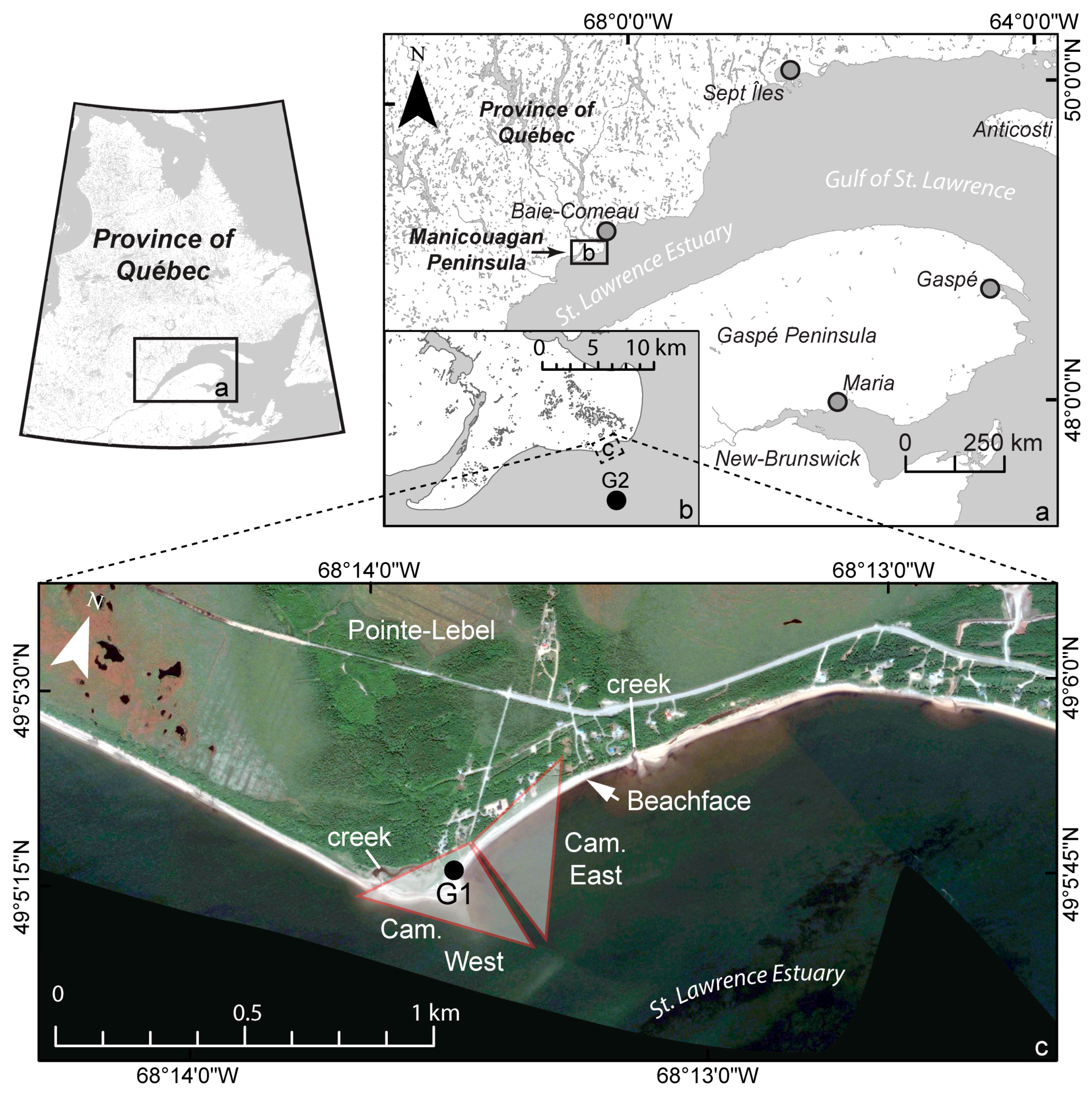
2.1. Study Area
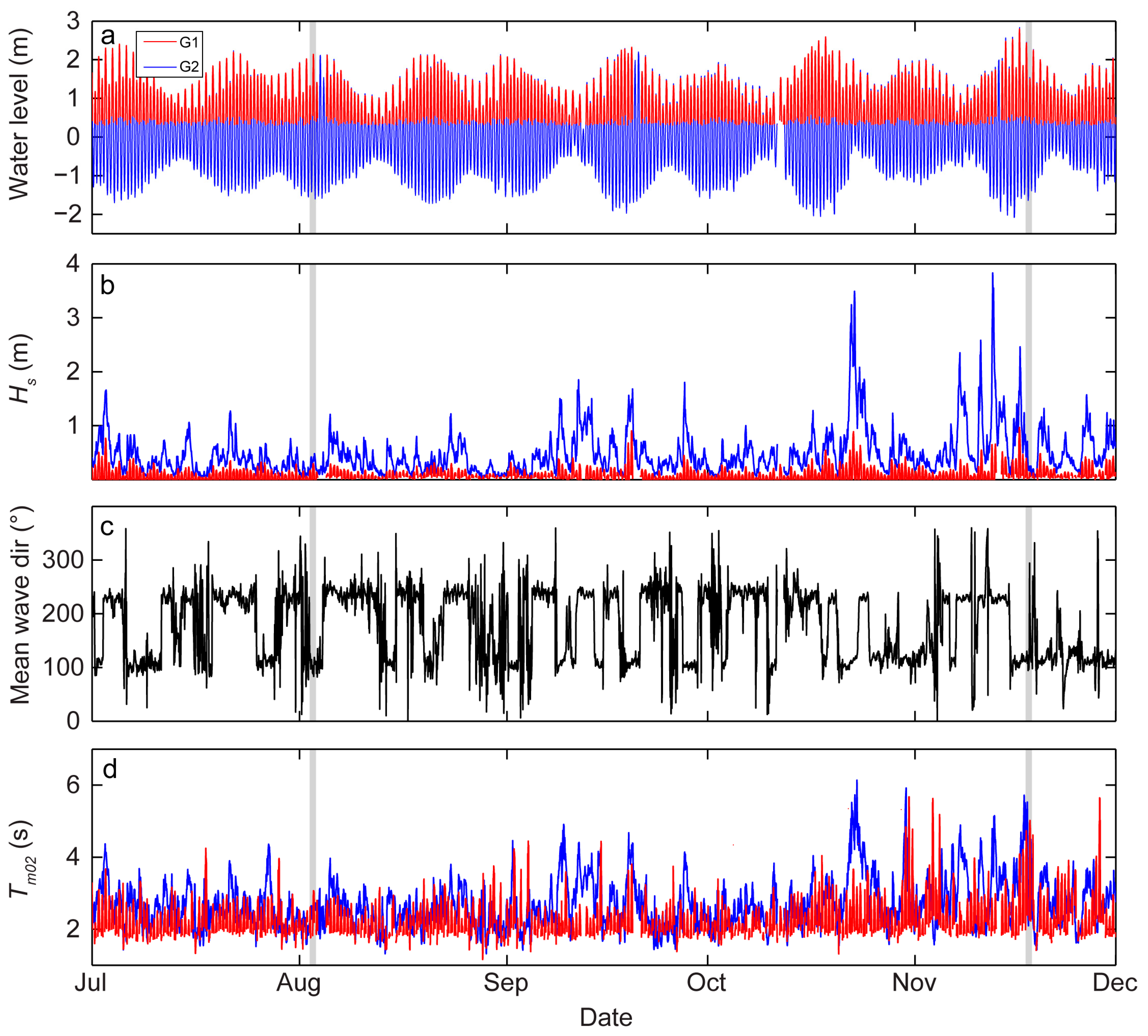
2.2. Wave and Tidal Data
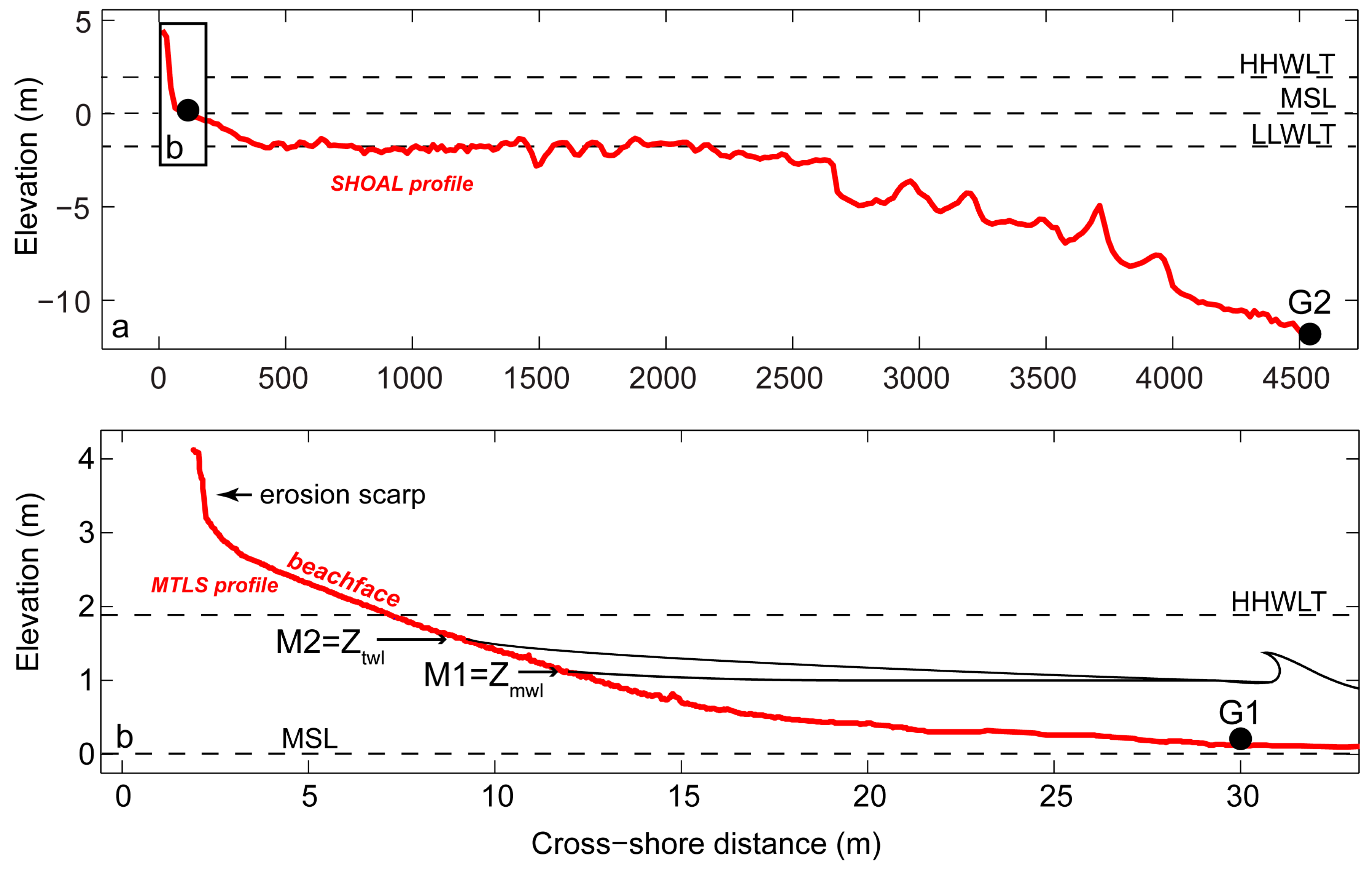
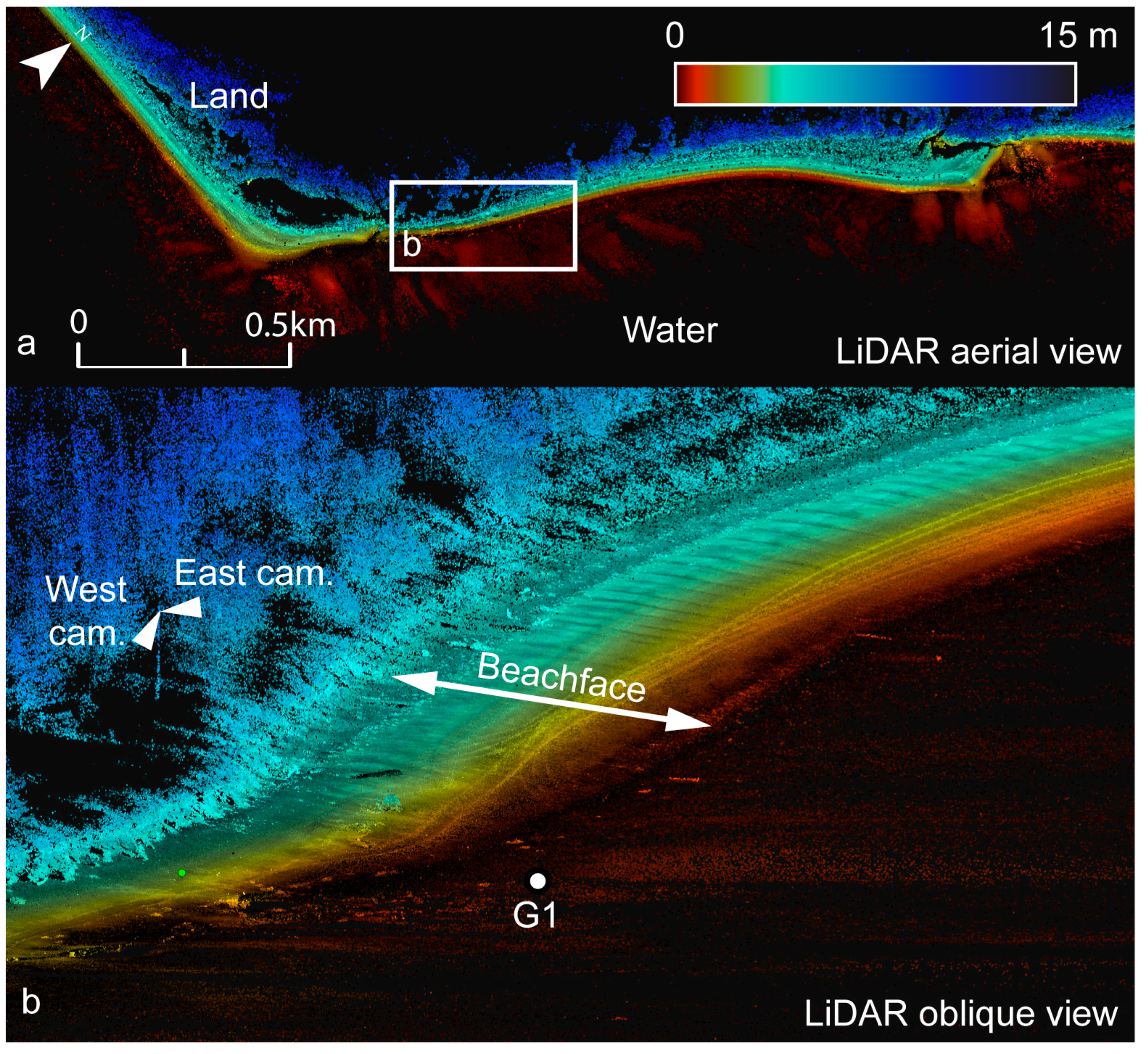
2.3. LiDAR Survey and Topographic Data
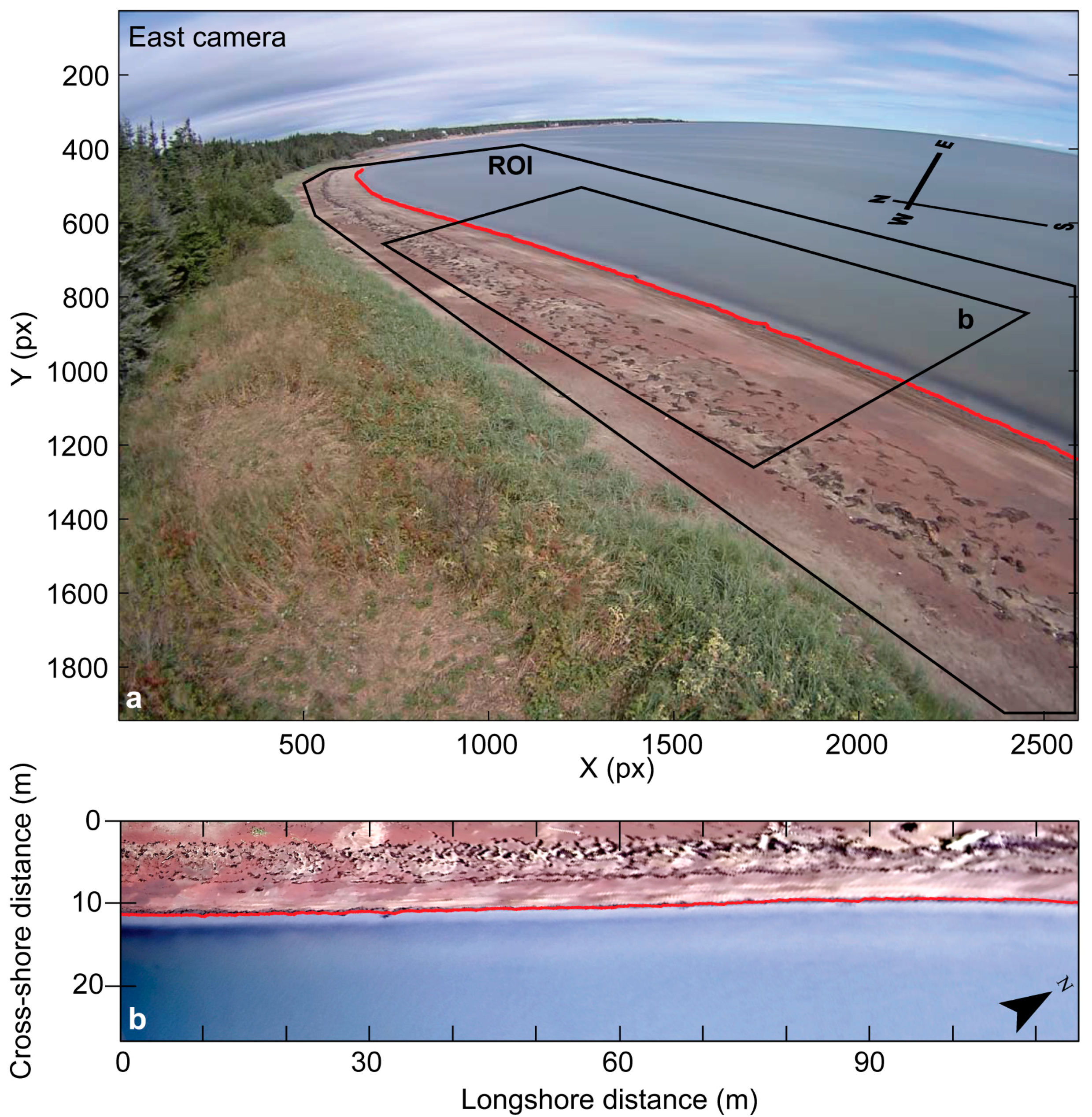
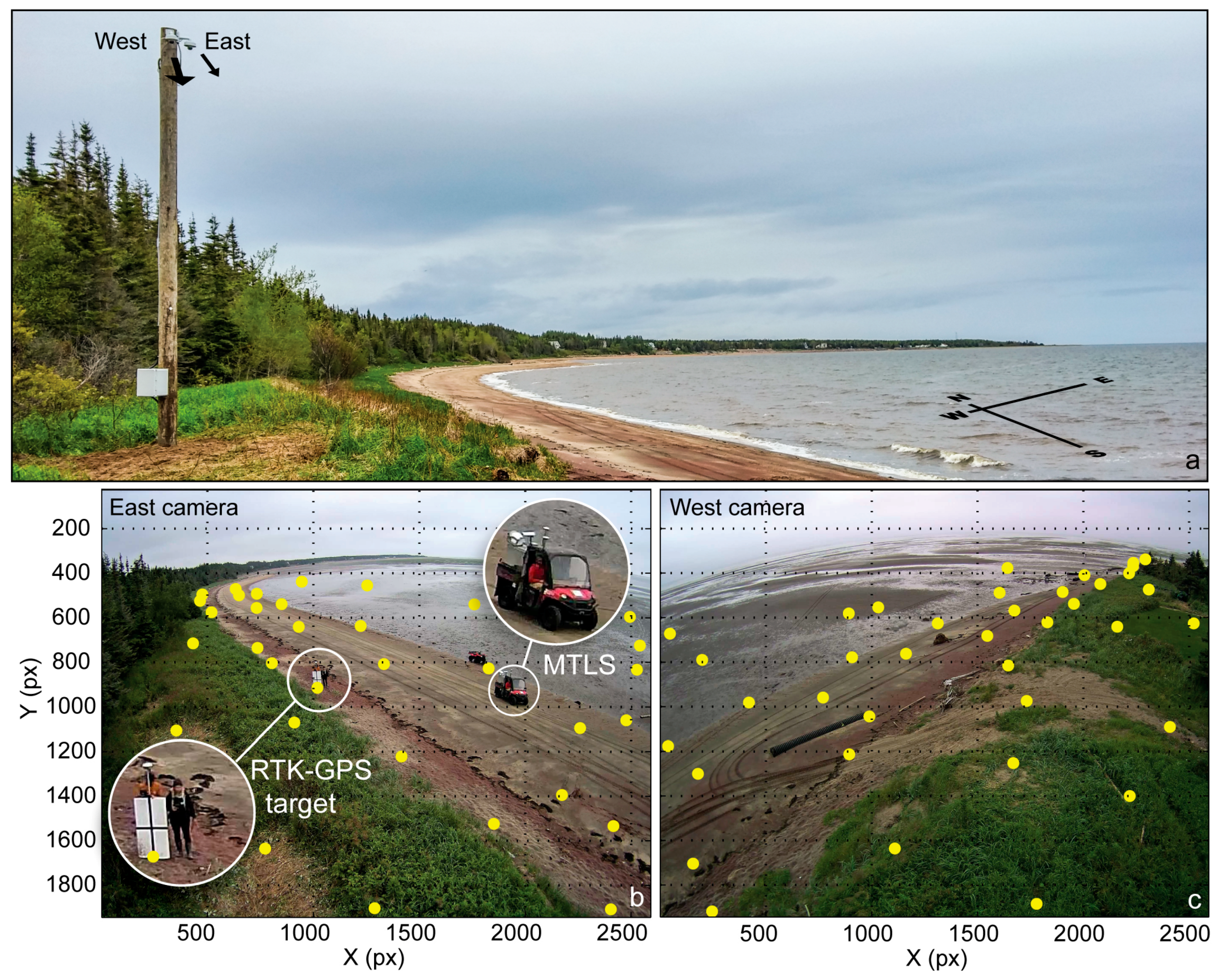
2.4. Video Monitoring Station
2.5. Cameras Calibration
2.6. Shoreline Detection and Water Elevation Models
3. Results and Discussion
3.1. Shoreline Detection and Elevation Analyses
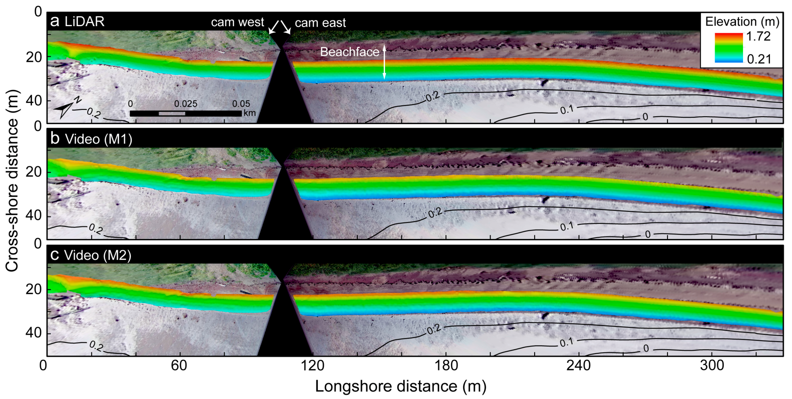
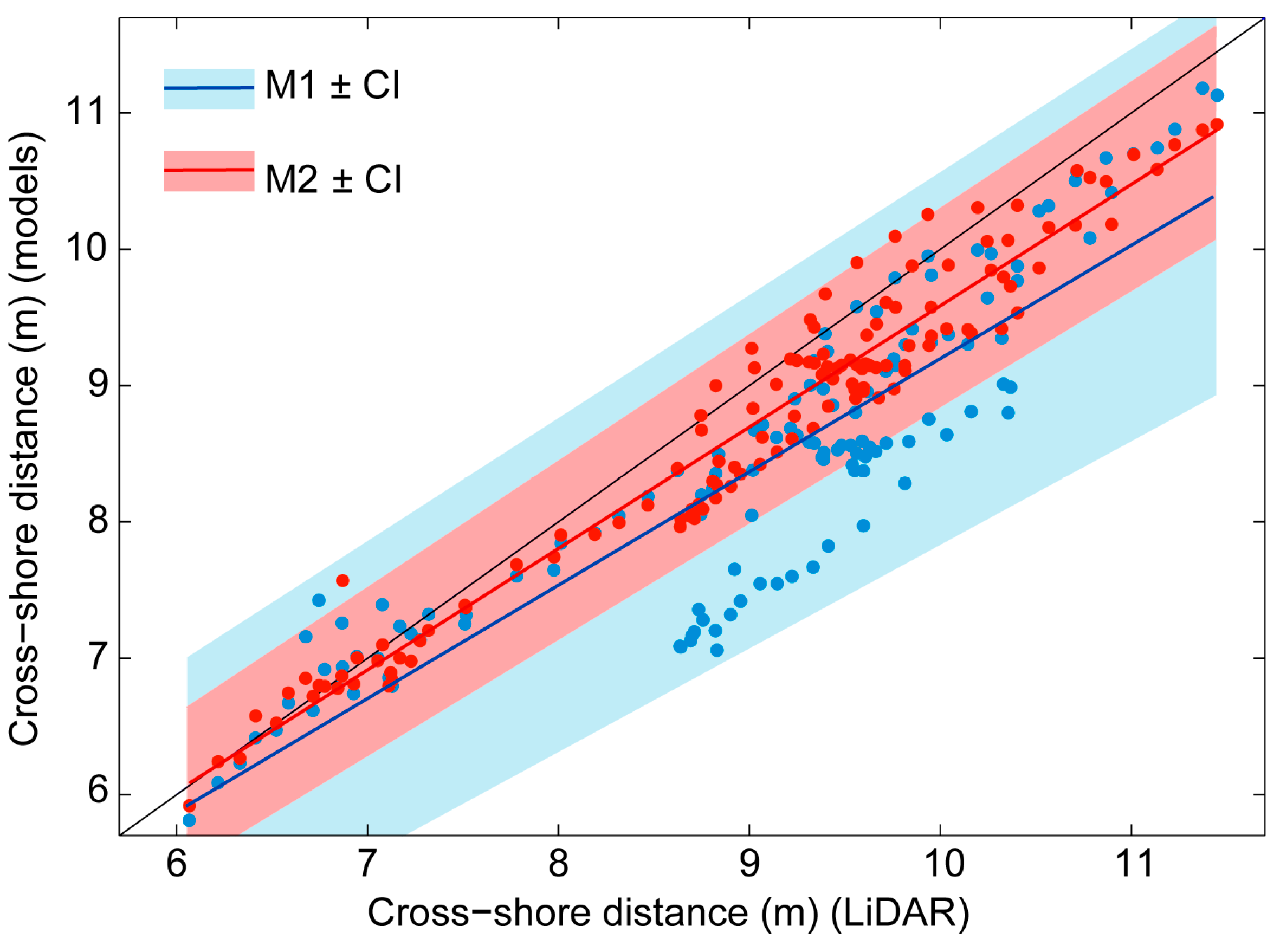
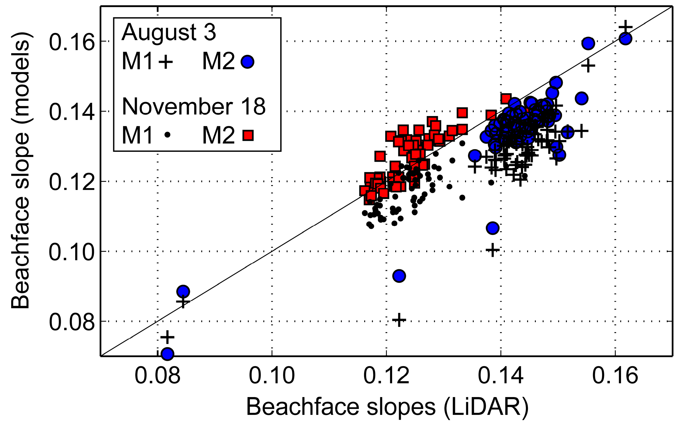
3.2. Comparing Video- to LiDAR-Based Topography
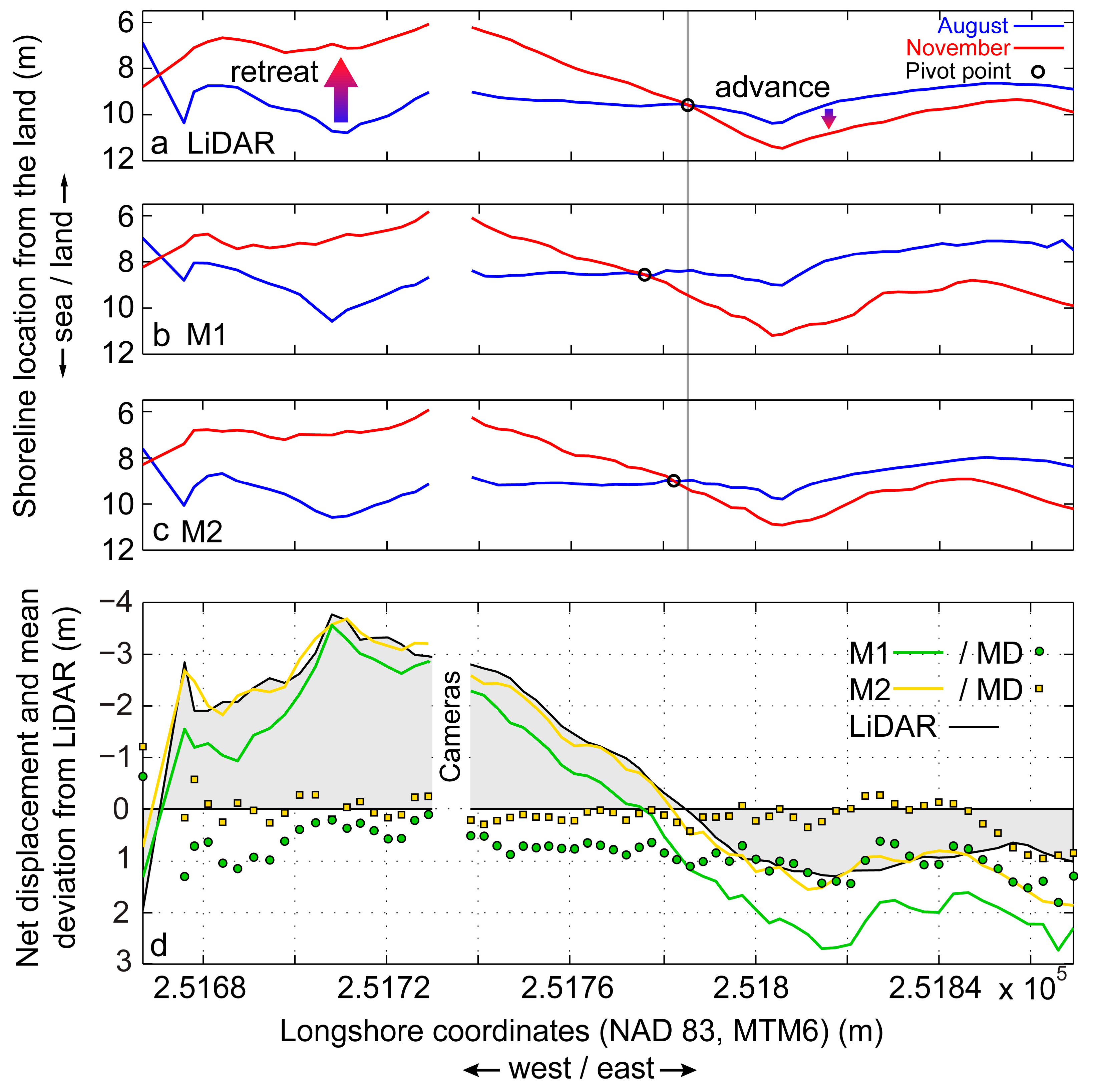
3.3. Cross-Shore Position of the Shoreline
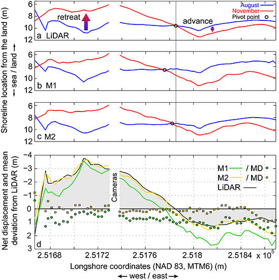
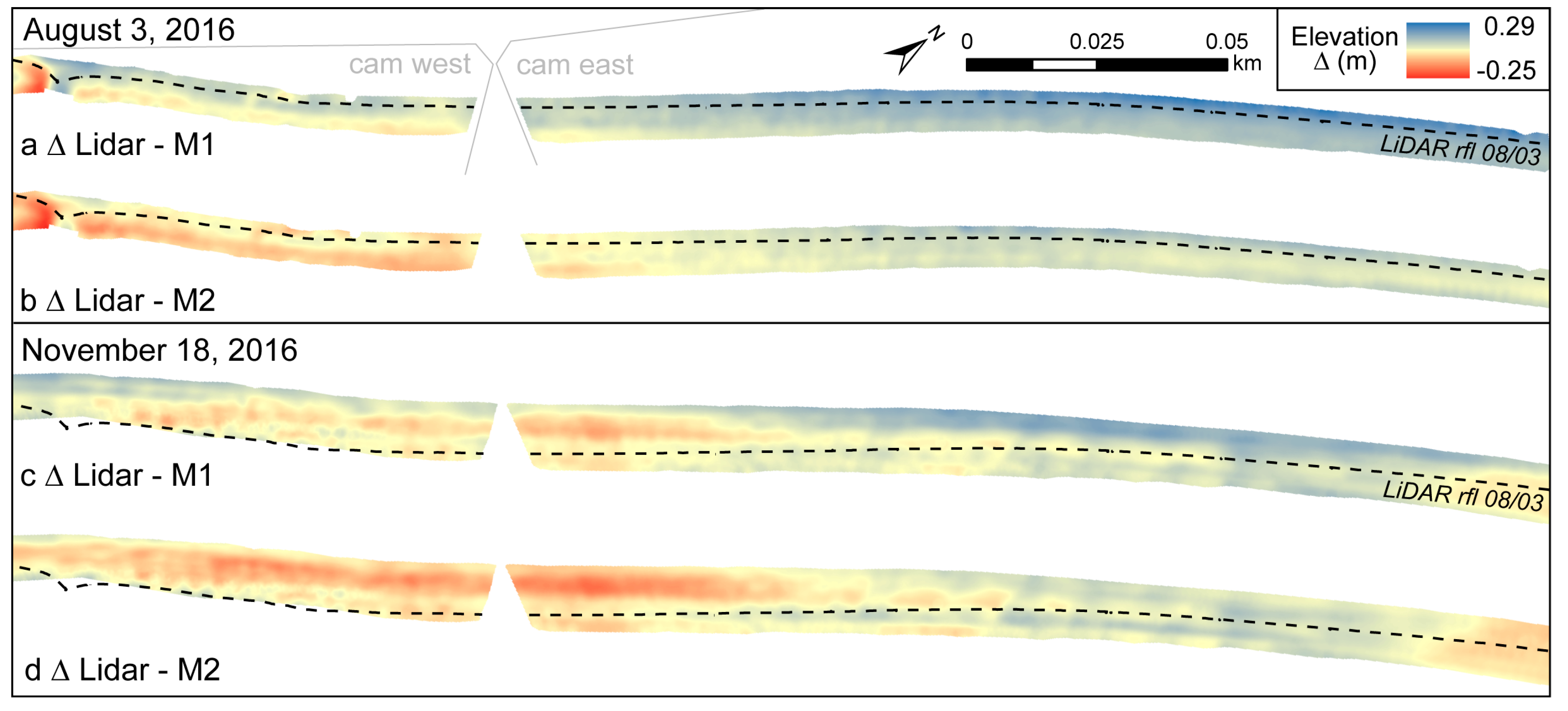
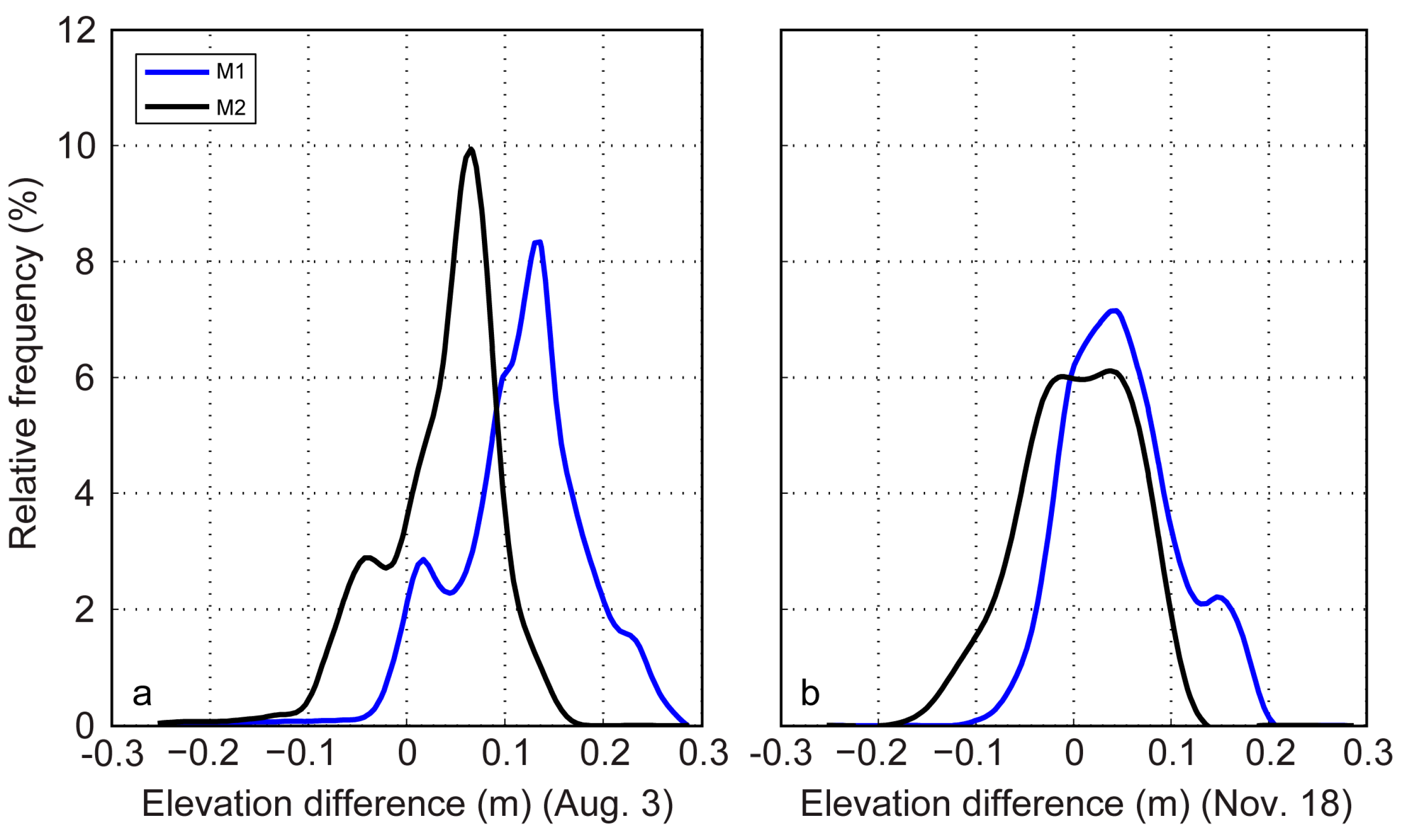
3.4. Spatiotemporal Analysis of the Morphological Evolution
3.5. Perpectives and Limitations
4. Conclusions
Acknowledgments
Author Contributions
Conflicts of Interest
References
- Masselink, G.; Puleo, J.A. Swash-zone morphodynamics. Cont. Shelf Res. 2006, 26, 661–680. [Google Scholar] [CrossRef]
- Ruessink, B.G.; Kleinhans, M.G.; van den Beukel, P.G.L. Observations of swash under highly dissipative conditions. J. Geophys. Res. Oceans 1998, 103, 3111–3118. [Google Scholar] [CrossRef]
- Sous, D.; Petitjean, L.; Bouchette, F.; Rey, V.; Meulé, S.; Sabatier, F.; Martins, K. Field evidence of swash groundwater circulation in the microtidal rousty beach, France. Adv. Water Resour. 2016, 97, 144–155. [Google Scholar] [CrossRef]
- Huisman, C.E.; Bryan, K.R.; Coco, G.; Ruessink, B.G. The use of video imagery to analyse groundwater and shoreline dynamics on a dissipative beach. Cont. Shelf Res. 2011, 31, 1728–1738. [Google Scholar] [CrossRef] [Green Version]
- Vousdoukas, M.I.; Velegrakis, A.F.; Dimou, K.; Zervakis, V.; Conley, D.C. Wave run-up observations in microtidal, sediment-starved pocket beaches of the Eastern Mediterranean. J. Mar. Syst. 2009, 78, S37–S47. [Google Scholar] [CrossRef]
- Yates, M.L.; Guza, R.T.; O’Reilly, W.C. Equilibrium shoreline response: Observations and modeling. J. Geophys. Res. 2009, 114, C09014. [Google Scholar] [CrossRef]
- Hardisty, J. A morphodynamic model for beach gradients. Earth Surf. Process. Landf. 1986, 11, 327–333. [Google Scholar] [CrossRef]
- Aagaard, T.; Black, K.P.; Greenwood, B. Cross-shore suspended sediment transport in the surf zone: A field-based parameterization. Mar. Geol. 2002, 185, 283–302. [Google Scholar] [CrossRef]
- Forbes, D.L.; Taylor, R.B. Ice in the shore zone and the geomorphology of cold coasts. Prog. Phys. Geogr. 1994, 18, 59–89. [Google Scholar] [CrossRef]
- Blossier, B.; Bryan, K.R.; Daly, C.J.; Winter, C. Spatial and temporal scales of shoreline morphodynamics derived from video camera observations for the island of Sylt, German Wadden Sea. Geo-Mar. Lett. 2016. [Google Scholar] [CrossRef]
- Bernatchez, P.; Fraser, C. Evolution of coastal defence structures and consequences for beach width trends, Québec, Canada. J. Coast. Res. 2012, 285, 1550–1566. [Google Scholar] [CrossRef]
- Trenhaile, A.S. Modeling the accumulation and dynamics of beaches on shore platforms. Mar. Geol. 2004, 206, 55–72. [Google Scholar] [CrossRef]
- Didier, D.; Bernatchez, P.; Marie, G.; Boucher-Brossard, G. Wave runup estimations on platform-beaches for coastal flood hazard assessment. Nat. Hazards 2016, 83, 1143–1467. [Google Scholar] [CrossRef]
- Floc’h, F.; Le Dantec, N.; Lemos, C.; Cancouët, R.; Sous, D.; Petitjean, L.; Bouchette, F.; Ardhuin, F.; Suanez, S.; Delacourt, C. Morphological response of a macrotidal embayed beach, Porsmilin, France. J. Coast. Res. 2016, 75, 373–377. [Google Scholar] [CrossRef]
- Tribbia, J.; Moser, S.C. More than information: what coastal managers need to plan for climate change. Environ. Sci. Policy 2008, 11, 315–328. [Google Scholar] [CrossRef]
- List, J.H.; Farris, A.S.; Sullivan, C. Reversing storm hotspots on sandy beaches: Spatial and temporal characteristics. Mar. Geol. 2006, 226, 261–279. [Google Scholar] [CrossRef]
- Cheng, J.; Wang, P.; Guo, Q. Measuring beach profiles along a low-wave energy microtidal coast, West-Central Florida, USA. Geosciences 2016, 6, 44. [Google Scholar] [CrossRef]
- Coco, G.; Senechal, N.; Rejas, A.; Bryan, K.R.; Capo, S.; Parisot, J.P.; Brown, J.A.; Macmahan, J.H.M. Beach response to a sequence of extreme storms. Geomorphology 2014, 204, 493–501. [Google Scholar] [CrossRef] [Green Version]
- Silveira, T.M.; Carapuço, A.M.; Sousa, H.; Taborda, R.; Psuty, N.P. Optimizing beach topographical field surveys: Matching the effort with the objectives. J. Coast. Res. 2013, 1, 588–593. [Google Scholar] [CrossRef]
- Suanez, S.; Cancouët, R.; Floc’h, F.; Blaise, E.; Ardhuin, F.; Filipot, J.-F.; Cariolet, J.-M.; Delacourt, C. Observations and predictions of wave runup, extreme water levels, and medium-term dune erosion during storm conditions. J. Mar. Sci. Eng. 2015, 3, 674–698. [Google Scholar] [CrossRef] [Green Version]
- McNinch, J.E. Bar and swash imaging radar (BASIR): A mobile X-band radar designed for mapping nearshore sand bars and swash-defined shorelines over large distances. J. Coast. Res. 2007, 231, 59–74. [Google Scholar] [CrossRef]
- Casella, E.; Rovere, A.; Pedroncini, A.; Mucerino, L.; Casella, M.; Cusati, L.A.; Vacchi, M.; Ferrari, M.; Firpo, M. Study of wave runup using numerical models and low-altitude aerial photogrammetry: A tool for coastal management. Estuar. Coast. Shelf Sci. 2014, 149, 160–167. [Google Scholar] [CrossRef]
- Mancini, F.; Dubbini, M.; Gattelli, M.; Stecchi, F.; Fabbri, S.; Gabbianelli, G. Using unmanned aerial vehicles (uav) for high-resolution reconstruction of topography: The structure from motion approach on coastal environments. Remote Sens. 2013, 5, 6880–6898. [Google Scholar] [CrossRef] [Green Version]
- Holman, R.A.; Brodie, K.L.; Spore, N.J. Surf zone characterization using a small quadcopter: Technical issues and procedures. IEEE Trans. Geosci. Remote Sens. 2017, 55, 2017–2027. [Google Scholar] [CrossRef]
- Vousdoukas, M.I.; Kirupakaramoorthy, T.; Oumeraci, H.; de la Torre, M.; Wübbold, F.; Wagner, B.; Schimmels, S. The role of combined laser scanning and video techniques in monitoring wave-by-wave swash zone processes. Coast. Eng. 2014, 83, 150–165. [Google Scholar] [CrossRef]
- Blenkinsopp, C.E.; Mole, M.A.; Turner, I.L.; Peirson, W.L. Measurements of the time-varying free-surface profile across the swash zone obtained using an industrial LIDAR. Coast. Eng. 2010, 57, 1059–1065. [Google Scholar] [CrossRef]
- Brodie, K.L.; Raubenheimer, B.; Elgar, S.; Slocum, R.K.; McNinch, J.E. Lidar and pressure measurements of inner-surfzone waves and setup. J. Atmos. Ocean. Technol. 2015, 32, 1945–1959. [Google Scholar] [CrossRef]
- Holman, R.; Stanley, J. The history and technical capabilities of Argus. Coast. Eng. 2007, 54, 477–491. [Google Scholar] [CrossRef]
- Pitman, S.J. Methods for field measurement and remote sensing of the swash zone. In Geomorphological Techniques; Cook, S.J., Clark, L.E., Nield, J.M., Eds.; British Society of Geomorphology: Oxford, UK, 2014; Volume 3, pp. 1–14. [Google Scholar]
- Almar, R.; Ibaceta, R.; Blenkinsopp, C.; Catalan, P.; Cienfuegos, R.; Trung Viet, N.; Hai Thuan, D.; Van Uu, D.; Lefebvre, J.-P.; Sowah Laryea, W.; et al. Swash-based wave energy reflection on natural beaches. Proc. Coast. Sediments 2015, 1–13. [Google Scholar] [CrossRef]
- Simarro, G.; Guedes, R.M.C.; Sancho, A.; Guillen, J.; Bryan, K.R.; Coco, G. On the use of variance images for runup and shoreline detection. Coast. Eng. 2015, 99, 136–147. [Google Scholar] [CrossRef]
- Senechal, N.; Coco, G.; Bryan, K.R.; Holman, R.A. Wave runup during extreme storm conditions. J. Geophys. Res. 2011, 116, C07032. [Google Scholar] [CrossRef]
- Stockdon, H.F.; Thompson, D.M.; Plant, N.G.; Long, J.W. Evaluation of wave runup predictions from numerical and parametric models. Coast. Eng. 2014, 92, 1–11. [Google Scholar] [CrossRef]
- Stockdon, H.; Holman, R.; Howd, P.; Sallenger, A. Empirical parameterization of setup, swash, and runup. Coast. Eng. 2006, 53, 573–588. [Google Scholar] [CrossRef]
- Vousdoukas, M.I.; Ferreira, Ó.; Almeida, L.P.; Pacheco, A. Toward reliable storm-hazard forecasts: XBeach calibration and its potential application in an operational early-warning system. Ocean Dyn. 2012, 62, 1001–1015. [Google Scholar] [CrossRef]
- Uunk, L.; Wijnberg, K.M.; Morelissen, R. Automated mapping of the intertidal beach bathymetry from video images. Coast. Eng. 2010, 57, 461–469. [Google Scholar] [CrossRef]
- Almar, R.; Senechal, N.; Coco, G. Estimation vidéo haute fréquence de la topographie inter- tidale d’une plage sableuse: Application à la caractérisation des seuils d’engraissement et d’érosion. In Xèmes Journées Nationales Génie Côtier—Génie Civil; Paralia: Sophia Antipolis, France, 2008; pp. 505–514. [Google Scholar]
- Almar, R.; Ranasinghe, R.; Sénéchal, N.; Bonneton, P.; Roelvink, D.J.A.; Bryan, K.R.; Marieu, V.; Parisot, J.-P.; Senechal, N.; Bonneton, P.; et al. Video-based detection of shorelines at complex meso-macro tidal beaches. J. Coast. Res. 2012, 28, 1040–1048. [Google Scholar] [CrossRef]
- Pearre, N.S.; Puleo, J.A. Quantifying seasonal shoreline variability at Rehoboth Beach, Delaware, using automated imaging techniques. J. Coast. Res. 2009, 254, 900–914. [Google Scholar] [CrossRef]
- Holman, R.; Sallenger, A.; Lippmann, T.; Haines, J. The application of video image processing to the study of nearshore processes. Oceanography 1993, 6, 78–85. [Google Scholar] [CrossRef]
- Bernatchez, P.; Dubois, J.-M.M. Seasonal quantification of coastal processes and cliff erosion on fine sediment shorelines in a cold temperate climate, north shore of the St. Lawrence maritime estuary, Québec. J. Coast. Res. 2008, 1, 169–180. [Google Scholar] [CrossRef]
- Aarninkhof, S.G.J.; Turner, I.L.; Dronkers, T.D.T.; Caljouw, M.; Nipius, L. A video-based technique for mapping intertidal beach bathymetry. Coast. Eng. 2003, 49, 275–289. [Google Scholar] [CrossRef]
- Plant, N.G.; Holman, R. A. Intertidal beach profile estimation using video images. Mar. Geol. 1997, 140, 1–24. [Google Scholar] [CrossRef]
- Madsen, A.J.; Plant, N.G. Intertidal beach slope predictions compared to field data. Mar. Geol. 2001, 173, 121–139. [Google Scholar] [CrossRef]
- Morris, B.D.; Coco, G.; Bryan, K.R.; Turner, I.L.; Street, K.; Vale, M. Video-derived mapping of estuarine evolution. J. Coast. Res. 2007, 2007, 410–414. [Google Scholar]
- Turner, I.L.; Leyden, V.M. System Description and Analysis of Shoreline Change: August 1999–February 2000. Report 1. Northern Gold Coast Coastal Imaging System; Water Research Laboratory: Manly Vale, NSW, Australia, 2000. [Google Scholar]
- Vousdoukas, M.I.; Ferreira, P.M.; Almeida, L.P.; Dodet, G.; Psaros, F.; Andriolo, U.; Taborda, R.; Silva, A.N.; Ruano, A.; Ferreira, Ó.M. Performance of intertidal topography video monitoring of a meso-tidal reflective beach in South Portugal. Ocean Dyn. 2011, 61, 1521–1540. [Google Scholar] [CrossRef]
- Plant, N.G.; Aarninkhof, S.G.J.; Turner, I.L.; Kingston, K.S. The performance of shoreline detection models applied to video imagery. J. Coast. Res. 2007, 23, 658–670. [Google Scholar] [CrossRef]
- Cariolet, J.-M.; Suanez, S. Runup estimations on a macrotidal sandy beach. Coast. Eng. 2013, 74, 11–18. [Google Scholar] [CrossRef]
- Melby, J.; Caraballo-Nadal, N.; Kobayashi, N. Wave runup prediction for flood mapping. In Proceedings of the Coastal Engineering, Santander, Spain, 1–6 July 2012; Volume 1, p. 79. [Google Scholar]
- Bernatchez, P.; Dubois, J.-M.M. Bilan des connaissances de la dynamique de l’érosion des côtes du Québec maritime laurentien. Géographie Phys. Quat. 2004, 58, 45. [Google Scholar] [CrossRef] [Green Version]
- Bernatchez, P. Évolution Littorale Holocène et Actuelle des Complexes Deltaïques de Betsiamites et de Manicouagan-Outardes: Synthèse, Processus, Causes et Perspectives. Ph.D. Thesis, Université Laval, Ville de Québec, QC, Canada, 2003. [Google Scholar]
- Duchesne, M.J.; Pinet, N.; Bédard, K.; St-Onge, G.; Lajeunesse, P.; Campbell, D.C.; Bolduc, A. Role of the bedrock topography in the Quaternary filling of a giant estuarine basin: The Lower St. Lawrence Estuary, Eastern Canada. Basin Res. 2010, 22, 933–951. [Google Scholar] [CrossRef]
- Pratte, S.; Garneau, M.; De Vleeschouwer, F. Late-Holocene atmospheric dust deposition in eastern Canada (St. Lawrence North Shore). Holocene 2016. [Google Scholar] [CrossRef]
- Senneville, S.; St-Onge Drouin, S.; Dumont, D.; Bihan-Poudec, M.-C.; Belemaalem, Z.; Corriveau, M.; Bernatchez, P.; Bélanger, S.; Tolszczuk-leclerc, S.; Villeneuve, R. Modélisation des Glaces dans L’estuaire et le Golfe du Saint-Laurent dans la Perspective des Changements Climatiques; Technical Report; Université du Québec à Rimouski: Rimouski, QC, Canada, 2014. [Google Scholar]
- Ruest, B.; Neumeier, U.; Dumont, D.; Bismuth, E.; Senneville, S.; Caveen, J. Recent wave climate and expected future changes in the seasonally ice-infested waters of the Gulf of St. Lawrence, Canada. Clim. Dyn. 2015. [Google Scholar] [CrossRef]
- CHS Canadian Tides and Water Levels Data Archives. Available online: http://www.isdm-gdsi.gc.ca/isdm-gdsi/twl-mne/index-eng.htm (accessed on 20 March 2015).
- Saucier, F.J.; Chassé, J. Tidal circulation and buoyancy effects in the St. Lawrence Estuary. Atmos. Ocean 2000, 38, 505–556. [Google Scholar] [CrossRef]
- Masselink, G.; Short, A.D. The effect of tide range on beach morphodynamics and morphology: A conceptual beach model. J. Coast. Res. 1993, 9, 785–800. [Google Scholar]
- Scott, T.; Masselink, G.; Russell, P. Morphodynamic characteristics and classification of beaches in England and Wales. Mar. Geol. 2011, 286, 1–20. [Google Scholar] [CrossRef] [Green Version]
- Dupuis, L.; Ouellet, Y. Prévision des vagues dans l’estuaire du Saint-Laurent à l’aide d’un modèle bidimensionnel. Can. J. Civ. Eng. 1999, 26, 713–723. [Google Scholar] [CrossRef]
- Didier, D.; Bernatchez, P.; Boucher-Brossard, G.; Lambert, A.; Fraser, C.; Barnett, R.; Van-Wierts, S. Coastal flood assessment based on field debris measurements and wave runup empirical model. J. Mar. Sci. Eng. 2015, 3, 560–590. [Google Scholar] [CrossRef]
- Stumpf, A.; Augereau, E.; Delacourt, C.; Bonnier, J. Photogrammetric discharge monitoring of small tropical mountain rivers: A case study at Rivière des Pluies, Réunion Island. Water Resour. Res. 2016, 52, 4550–4570. [Google Scholar] [CrossRef]
- Harley, M.D.; Turner, I.L.; Short, A.D.; Ranasinghe, R. Assessment and integration of conventional, RTK-GPS and image-derived beach survey methods for daily to decadal coastal monitoring. Coast. Eng. 2011, 58, 194–205. [Google Scholar] [CrossRef]
- Bracs, M.A.; Turner, I.L.; Splinter, K.D.; Short, A.D.; Lane, C.; Davidson, M.A.; Goodwin, I.D.; Pritchard, T.; Cameron, D. Evaluation of opportunistic shoreline monitoring capability utilizing existing “surfcam” infrastructure. J. Coast. Res. 2016, 319, 542–554. [Google Scholar] [CrossRef]
- Angnuureng, D.B.; Almar, R.; Senechal, N.; Castelle, B.; Addo, K.A.; Marieu, V.; Ranasinghe, R. Shoreline resilience to individual storms and storm clusters on a meso-macrotidal barred beach. Geomorphology 2017, 290, 265–276. [Google Scholar] [CrossRef]
- Poate, T.G.; McCall, R.T.; Masselink, G. A new parameterisation for runup on gravel beaches. Coast. Eng. 2016, 117, 176–190. [Google Scholar] [CrossRef]
- Ojeda, E.; Guillén, J. Shoreline dynamics and beach rotation of artificial embayed beaches. Mar. Geol. 2008, 253, 51–62. [Google Scholar] [CrossRef]
- Abessolo Ondoa, G.; Almar, R.; Kestenare, E.; Bahini, A.; Houngue, G.-H.; Jouanno, J.; Du Penhoat, Y.; Castelle, B.; Melet, A.; Meyssignac, B.; et al. Potential of video cameras in assessing event and seasonal coastline behaviour: Grand Popo, Benin (Gulf of Guinea). J. Coast. Res. 2016, 75, 442–446. [Google Scholar] [CrossRef]
- McCarroll, R.J.; Brander, R.W.; Turner, I.L.; Leeuwen, B. Van Shoreface storm morphodynamics and mega-rip evolution at an embayed beach: Bondi Beach, NSW, Australia. Cont. Shelf Res. 2016, 116, 74–88. [Google Scholar] [CrossRef]
- Blossier, B.; Bryan, K.R.; Daly, C.J.; Winter, C. Nearshore sandbar rotation at single-barred embayed beaches. J. Geophys. Res. Oceans 2016, 121, 2286–2313. [Google Scholar] [CrossRef]
- Wright, L.D.; Short, A.D. Morphodynamic variability of surf zones and beaches: A synthesis. Mar. Geol. 1984, 56, 93–118. [Google Scholar] [CrossRef]


| Analysis | Model Fit | Model Skill | ||||
|---|---|---|---|---|---|---|
| R2 | RMSE | MD | MAD | |||
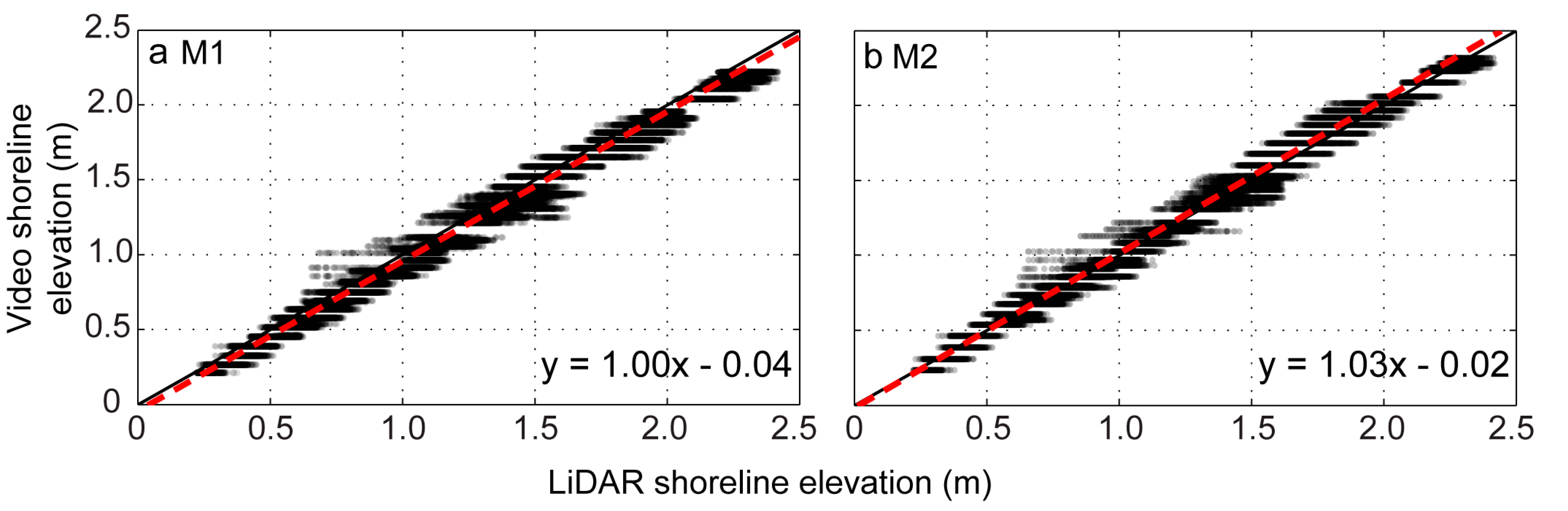
| Shoreline detection (Δz) | M1~LiDAR | 1.00x − 0.04 | 0.99 | 0.06 | −0.04 | 0.06 |
| M2~LiDAR | 1.03x − 0.02 | 0.99 | 0.06 | 0.02 | 0.05 | |
| Cross-shore location (Δy) (same date) | M1~LiDAR | 0.83x + 0.90 | 0.81 | 0.52 | 0.63 | 0.66 |
| M2~LiDAR | 0.89x + 0.68 | 0.95 | 0.27 | 0.31 | 0.36 | |
| Cross-shore displacements (Δy) (multi-dates) | M1~LiDAR | 1.11x + 0.92 | 0.97 | 0.35 | 0.83 | 0.85 |
| M2~LiDAR | 1.02x + 0.12 | 0.97 | 0.33 | 0.11 | 0.24 | |
| Beachface slopes (Δtan βbf) (August) | M1~LiDAR | 0.95x + 0.006 | 0.73 | 0.007 | 0.014 | |
| M2~LiDAR | 0.99x − 0.007 | 0.79 | 0.006 | 0.008 | ||
| (November) | M1~LiDAR | 0.64x + 0.04 | 0.39 | 0.005 | 0.007 | |
| M2~LiDAR | 1.02x | 0.66 | 0.004 | 0.004 | ||
© 2017 by the authors. Licensee MDPI, Basel, Switzerland. This article is an open access article distributed under the terms and conditions of the Creative Commons Attribution (CC BY) license (http://creativecommons.org/licenses/by/4.0/).
Share and Cite
Didier, D.; Bernatchez, P.; Augereau, E.; Caulet, C.; Dumont, D.; Bismuth, E.; Cormier, L.; Floc’h, F.; Delacourt, C. LiDAR Validation of a Video-Derived Beachface Topography on a Tidal Flat. Remote Sens. 2017, 9, 826. https://doi.org/10.3390/rs9080826
Didier D, Bernatchez P, Augereau E, Caulet C, Dumont D, Bismuth E, Cormier L, Floc’h F, Delacourt C. LiDAR Validation of a Video-Derived Beachface Topography on a Tidal Flat. Remote Sensing. 2017; 9(8):826. https://doi.org/10.3390/rs9080826
Chicago/Turabian StyleDidier, David, Pascal Bernatchez, Emmanuel Augereau, Charles Caulet, Dany Dumont, Eliott Bismuth, Louis Cormier, France Floc’h, and Christophe Delacourt. 2017. "LiDAR Validation of a Video-Derived Beachface Topography on a Tidal Flat" Remote Sensing 9, no. 8: 826. https://doi.org/10.3390/rs9080826