Determinants of Aboveground Biomass across an Afromontane Landscape Mosaic in Kenya
by
 , , , , and
Hari Adhikari
1,* ,
,
Janne Heiskanen
1 ,
,
Mika Siljander
1,
Eduardo Maeda
2,
Vuokko Heikinheimo
1 and
Petri K. E. Pellikka
1 1
Department of Geosciences and Geography, University of Helsinki, P.O. Box 68, FI-00014 Helsinki, Finland
2
Fisheries and Environmental Management Group, Department of Environmental Sciences, University of Helsinki, P.O. Box 65, FI-00014 Helsinki, Finland
*
Author to whom correspondence should be addressed.
Remote Sens. 2017, 9(8), 827; https://doi.org/10.3390/rs9080827
Submission received: 21 June 2017
/
Revised: 4 August 2017
/
Accepted: 7 August 2017
/
Published: 11 August 2017
(This article belongs to the Special Issue Biomass Remote Sensing in Forest Landscapes)
Abstract
:Afromontane tropical forests maintain high biodiversity and provide valuable ecosystem services, such as carbon sequestration. The spatial distribution of aboveground biomass (AGB) in forest-agriculture landscape mosaics is highly variable and controlled both by physical and human factors. In this study, the objectives were (1) to generate a map of AGB for the Taita Hills, in Kenya, based on field measurements and airborne laser scanning (ALS), and (2) to examine determinants of AGB using geospatial data and statistical modelling. The study area is located in the northernmost part of the Eastern Arc Mountains, with an elevation range of approximately 600–2200 m. The field measurements were carried out in 215 plots in 2013–2015 and ALS flights conducted in 2014–2015. Multiple linear regression was used for predicting AGB at a 30 m × 30 m resolution based on canopy cover and the 25th percentile height derived from ALS returns (R2 = 0.88, RMSE = 52.9 Mg ha−1). Boosted regression trees (BRT) were used for examining the relationship between AGB and explanatory variables at a 250 m × 250 m resolution. According to the results, AGB patterns were controlled mainly by mean annual precipitation (MAP), the distribution of croplands and slope, which explained together 69.8% of the AGB variation. The highest AGB densities have been retained in the semi-natural vegetation in the higher elevations receiving more rainfall and in the steep slope, which is less suitable for agriculture. AGB was also relatively high in the eastern slopes as indicated by the strong interaction between slope and aspect. Furthermore, plantation forests, topographic position and the density of buildings had a minor influence on AGB. The findings demonstrate the utility of ALS-based AGB maps and BRT for describing AGB distributions across Afromontane landscapes, which is important for making sustainable land management decisions in the region.

1. Introduction
Afromontane tropical forests are globally important ecosystems, which maintain high biodiversity and provide valuable ecosystem services, such as carbon sequestration [1]. Tropical forests store large amounts of carbon, but due to forest degradation and deforestation, they can emit carbon to the atmosphere and boost global warming [2]. It tropical countries, such as Kenya, forests are under constant pressure because of increasing demand for food and shelter [3]. In East Africa, between 2002 and 2008, wooded vegetation cover decreased in area by 5.1%, 15.8% and 19.4% from forests, woodland and shrubland, respectively [4].
Hence, mapping above ground biomass (AGB) is an essential task for monitoring carbon stocks and dynamics across tropical African landscapes. Measuring AGB is also required for implementing payments for ecosystem services schemes and the United Nations Reducing Emissions from Deforestation and Forest Degradation (REDD+) mechanism [5]. Furthermore, AGB maps can be used for studying the determinants that control AGB distribution [6], which is important for the management of carbon stocks and understanding how carbon stocks might change in the future.
Field measurements provide accurate information about AGB, but sampling can be spatially limited due to difficult terrain or lacking resources. Remote sensing provides a cost-efficient alternative to mapping the wall-to-wall distribution of AGB across landscapes. Nonetheless, the use of optical satellite imagery for AGB mapping is often hindered by frequent cloud coverage. Furthermore, over dense crown covers, the data obtained by optical sensors may have limited capabilities in describing vegetation structure, as most spectral information is retrieved from the topmost parts of the canopy [2]. Radar sensors also have critical limitations in assessing AGB over tropical regions, given that their sensitivity to AGB variation decreases in the old-growth forests [7]. On the other hand, light detection and ranging (LiDAR) systems offer three-dimensional information on canopy structure that is better suited for AGB modelling than optical or radar imagery [8]. In particular, airborne laser scanning (ALS) has been found to be useful for estimating forest biophysical parameters, such as leaf area index (LAI), canopy height, canopy cover and AGB (e.g., [8,9]).
Although ALS has been used increasingly for AGB estimation and mapping in Africa [10,11,12], most studies to date have focused on tropical forests (e.g., [11,13]). However, tropical African landscapes are typically mosaics of multiple land uses, and a large fraction of landscape-level AGB can be located outside the forests [14]. For example, [15] determined mean AGB densities for land cover classes using samples of ALS data and a satellite image-based land cover map. Nevertheless, the distribution of AGB is highly variable, even under the same climatic condition and land use types [16,17]. Under these circumstances, wall-to-wall ALS coverage provides unique possibilities to recover spatial variations in AGB patterns.
Furthermore, ALS-based AGB maps can be paired with other geospatial data to study the fundamental biotic and abiotic determinants of AGB [6,18,19]. Digital elevation models (DEM), climate data, land use and land cover maps and soil databases are commonly used for this purpose [6,16,18,19,20]. Although the underlining mechanisms of the relationships between large-scale drivers (e.g., climate variables) and AGB are currently better understood [21], the landscape scale drivers of the spatial distribution of AGB are still poorly understood. For instance, while the relationships between topography, biophysical factors, climate and AGB have been evaluated in previous studies, inconsistent results were observed in different ecosystems.
The objectives of this study were to (1) generate an AGB map for the Taita Hills using ALS and (2) examine the determinants of AGB using geospatial datasets on topography, soils, climate, land use and statistical modelling at the landscape to the regional scale. The Taita Hills, in southeastern Kenya, provide a unique setting to address our objectives. In a relatively small area, with large topographic variations, the landscape is characterized by a complex land cover mosaic, with large local variations in AGB.
2. Materials and Methods
2.1. Study Area
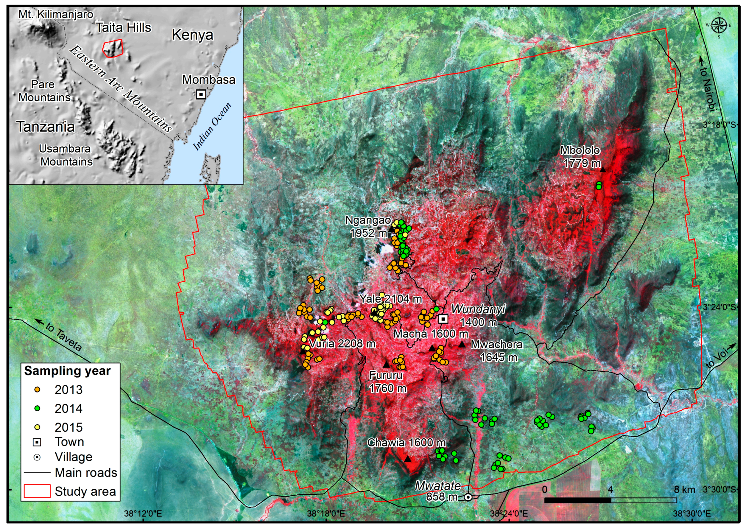
The Taita Hills (study area ca. 55,000 ha) in southeast Kenya are part of the Eastern Arc Mountains (Figure 1). The highest hilltop (Vuria) reaches 2208 meters above sea level (m a.s.l.). The hills are surrounded by semi-arid scrublands and dry savannas at an elevation of 600–900 m a.s.l. Due to the altitude difference, the hills experience a lower mean annual temperature (18.2 °C) compared with the lowlands (24.6 °C) [22]. The region has a bimodal rainfall pattern: long rains from March–May/June and short rains from October–December. Mean annual precipitations between 1986 and 2003 were 1132 mm at 1768 m a.s.l (Mgange) and 587 mm at 560 m a.s.l. (Voi) [23]. The higher elevations receive more rain because of the orographic rainfall pattern, while the northwestern slope in the rain-shadow receives less precipitation compared with the southeastern slope [3].
The area belongs to one of the world’s most important biodiversity hotspots [1] and hosts some remaining indigenous montane forests [24]. The landscape is a highly fragmented mosaic of montane forest patches, exotic plantations and agriculture with agroforestry and horticulture being common [25]. According to [15], the main land use and land cover types in 2011 were cropland (40.5%), thicket (28.9%), shrubland (12.8%), woodland and agroforestry (10.7%), plantation forest (4.6%), indigenous montane forest (1.4%) and bare rock, soil and built-up areas (1.1%). Agricultural expansion has been taking place in the area for decades. Since 1987, cropland area has increased at the expense of thickets and shrublands in the foothills and lowlands, while the hills were taken to agriculture before the 1950s and after [23,24].
The remnant montane forests can be separated into lower and upper montane forests. The lower montane forests are taller and drier compared with the elfin forest like upper montane forests, which receive significant amounts of precipitation through a mist. These mist forests on the top of Vuria, have typically only one layer and are covered by epiphytic mosses and lichens [26,27].
Common tree species in the montane forests include Tabernaemontana stapfiana, Macaranga capensis, Psychotria petitii, Xymalos monospora, Prunus africana, Maesa lanceolata and Albizia gummifera, while Eucalyptus spp., Cupressus lusitanica and Pinus spp. are the main tree species in the plantations. In the lowlands, common tree species include Albizia amara, Sterculia africana, Lannea alata, Acacia tortilis, Commiphora africana and Commiphora incisa. Rocky and sandy areas outside the forests are dominated by Acacia mearnsii, while typical agroforestry species in the hills are Grevillea robusta and Persea americana and Mangifera indica in the lowlands [28,29].
2.2. Field Measurements and Aboveground Biomass Computations
The field measurements from a total of 215 circular 0.1-ha sample plots (radius 17.84 m) were used in this study for AGB modelling (Figure 1). The sampling design depended on the field campaign and sampling year. In 2013 and 2014, 150 plots were sampled randomly within 100-ha clusters in the hills and lowlands. In addition, 65 plots were sampled subjectively from high-biomass forest areas in 2014 and 2015. Sampling in the forest was guided by the ALS data [31] and visible to near-infrared imaging spectroscopy data (AisaEAGLE) [32] acquired in 2013 in order to cover variation in canopy structure and tree species composition.
Sample plot centers were positioned using a Trimble GeoXH GNSS receiver, and differential correction was made using a GNSS base station setup close to the town of Wundanyi (Figure 1). The slope in field plots varied from 0–50.5°. Slope correction was done either in the field in order to keep the plot area constant (i.e., 0.1 ha), or sample plot areas were corrected based on mean slope computed from ALS-derived DEM.
All of the tree stems with a diameter (D) at breast height (1.3 m) ≥10 cm were measured for D [18,20], and tree species were identified by a local para-taxonomist. In 2013, tree height (H) was measured for the majority of the trees outside forests by a clinometer, but only random measurements were made in the forests. In 2014 and 2015, H was measured using a laser range finder for at least three trees in each plot (i.e., the tree with minimum, maximum and median D) [32]. Furthermore, H was measured for all of the palms. For trees with only D measurement, H was predicted using a two-parameter Curtis height function [33]. Non-linear mixed effect modelling and the plot as random effects (e.g., [34]) were used to calibrate the H-D model for each sample plot. The ‘nlme’ package [35] in the R statistical software [36] was used to fit the model (RMSE 1.47 m, 22.6%).
In total, 6337 trees belonging to 141 species were measured. Tree species-specific equations are poorly available for the species-rich study area (e.g., [37]). However, generic species-specific models were used for Acacia spp., Eucalyptus spp., Pinus spp. and palms [37,38,39]; for the rest of the species, the AGB (kg) was computed based on wood-specific density (ρ, g cm−3), D (cm) and H (m) by the pantropical allometric model of [40]. Values of ρ were obtained from the global wood density databases [41,42]. Genus level averages were used for the species that lacked species-specific values, and if such could not be derived, a site-averaged value was used. Based on the tree-wise AGB estimates, AGB was calculated for the plots. Descriptive statistics for the field plots are given in Table 1.
2.3. Airborne Laser Scanning Data
ALS flights were conducted during several periods in 2014–2015 (Table 2). The data were provided as pre-processed and georeferenced point clouds. LAStools software (rapidlasso GmbH) was used to classify ground, building and vegetation returns and to create 2-m (for normalizing height) and 5-m (for explanatory variables) resolution DEMs. Triangular irregular network (TIN) interpolation was used for interpolating between the ground points [43].
The ALS point cloud elevations were normalized to heights above the ground surface by using the 2-m resolution DEM. Based on the normalized heights, noisy returns (e.g., high points) and returns from the electric lines were identified and removed manually.
2.4. Aboveground Biomass Mapping
The vegetation returns were further analyzed using FUSION software [44]. For modelling, various ALS metrics representing return height distribution and canopy cover were computed for the plots (Table 3). A 3-m threshold was used to separate understory and ground returns from canopy returns. This threshold was considered to match well with the minimum D used in the field measurements (i.e., 10 cm). For prediction, spatial grids of ALS metrics were generated at a spatial resolution of 30 m × 30 m. The spatial resolution of ALS metrics was determined by the sample plot size (0.1 ha). The correlation coefficients among the ALS metrics are shown in Figure A1.
General models for modelling AGB from ALS metrics are available (e.g., [45,46]). To obtain the highest possible accuracy to map AGB in the study area, the linear regression models were fit using the ‘lm’ function in R, and the ‘regsubsets’ function in the package ‘leaps’ [9,47] was used for exhaustive search of the best models having 1–4 predictors. The coefficient of determination (R2) and the root mean square error (RMSE) were used to evaluate the AGB models. The models were validated using leave-one-out cross-validation. The best model was selected based on the lowest Akaike’s information criterion and variance inflation factor (VIF < 4) [48].
2.5. Explanatory Variables for Modelling Distribution of Aboveground Biomass
A range of explanatory variables was derived from geospatial datasets for modelling AGB. Table 4 presents the complete list of variables.
The topographical and hydrological variables were derived from ALS-based DEM (5 m × 5 m cell). Higher spatial resolution (5 m) was used as the spatial resolution of ALS metrics was considered too coarse for topographic modelling. Slope, aspect, topographic position index (TPI), topographic wetness index (TWI) and river network were computed using System for Automated Geoscientific Analyses (SAGA) GIS (v. 2.1.2). The default settings were used if not stated otherwise. Slope (°) and aspect (°) were created using the ‘slope, aspect, curvature’ module. TPI is the difference between the elevation of a cell and the mean elevation of the cells in a neighborhood or within a specified radius around it. Positive values represent ridges, negative values valleys, and near zero values are either flat or have a constant slope [49]. Six radii between 50 m and 500 m were tested to cover local and landscape-scale variation in the ‘topographic position index’ module [50]. TWI was calculated using the ‘SAGA wetness index’ module [51]. River networks were extracted using the ‘channel network’ module, which requires elevation and catchment area as input. Catchment area was computed using the ‘catchment area (flow tracing)’ module [52], and the initiation type greater than 100,000 was used for channel network calculation. Soil type was derived from the Soil Atlas of Africa in the vector format [53]. Soil types included calcaric fluvisols (FL), rhodic ferralsols (FR), rendzic leptosols (LP), chromic luvisols (LV) and cambic umbrisols (UM).
Climatic variables included mean annual temperature (°C) and mean annual precipitation (mm), which were derived from [54] and [23], respectively. Temperatures were collected using small data loggers, which were placed at a height of 1.5 m at 40 sites covering different elevation zones and land cover types from dry, lowlands savannas to humid montane forest [54]. A 20-m resolution grid of mean annual precipitation (MAP) data was produced by interpolating monthly rainfall records of 11 ground stations in the Taita Hills from 1987–2005 using the procedures from the ANUSPLINE [55] package [23].
Land use classes (extent of croplands and plantation forest) were extracted from the most recent land use and land cover classification for the area [15,56]. A SPOT 4 HRVIR satellite image from October 2011 with a pixel size of 20 m × 20 m has been used for the classification with ten classes. The distribution of buildings was based on the ALS point clouds ’building’ class. Misclassified buildings were removed manually with the help of high-resolution satellite imagery available as the base map in ArcGIS [57]. Furthermore, the intensity image from ALS and the same imagery were used for digitizing the main roads. The correlation coefficients among the explanatory variables are shown in Figure A2 (Appendix).
Finally, the AGB map and all of the explanatory variables were aggregated to a 250 m × 250 m cell size for analysis. This was done in order to reduce uncertainties in AGB predictions [6] and explanatory variables and to better capture the landscape- and regional-scale impacts of explanatory variables on AGB.
2.6. Statistical Analysis
Boosted regression trees (BRT) [58] were used for examining the relationship between AGB and the explanatory variables. BRT improves the predictive performance by combining many simple models. BRT combines the strength of two algorithms: (1) regression trees and (2) boosting [58]. BRT can fit complex nonlinear relationships, and there is no need for prior data transformation. BRT had been used in similar studies for analyzing the effect of topography on biomass (e.g., [59]).
In order to reduce spatial autocorrelation, 25% of the cells were systematically sampled before statistical analysis. Correlations between the explanatory variables were studied, and highly correlated variables were excluded based on the Pearson correlation coefficient (|r| > 0.7) [60]. Among the correlated explanatory variables, the variable with the strongest univariate relationship with the response variable was retained [20]. The mean annual temperature (MAT) and elevation were correlated with MAP and hence removed (Appendix A). Furthermore, TWI was correlated with the slope. TPIs were correlated with each other, and the TPI500 having the strongest univariate relationship with AGB was retained.
BRT analysis was done using the ‘dismo’ package [61] in R. The Gaussian error distribution was used. Furthermore, the minimum predictive error was achieved when using a learning rate of 0.008, a tree complexity (interaction depth) of 7, a bag fraction of 0.5 and the tolerance method ‘fixed’.
3. Results
3.1. Aboveground Biomass Map
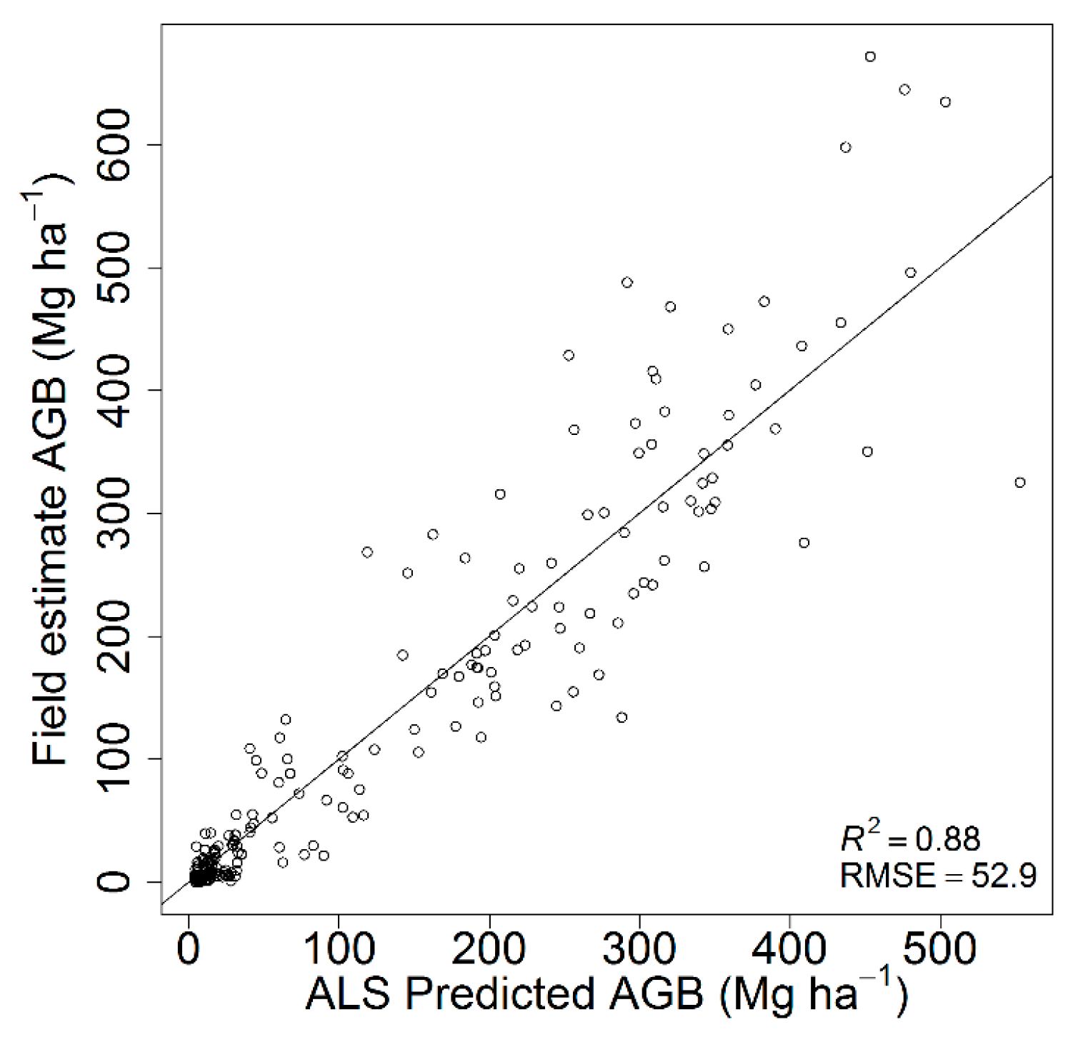
The best AGB model was fitted with an R2 of 0.88 and RMSE of 52.9 Mg⋅ha−1 based on the 25th percentile of height values (H.p25) and canopy cover (CC.all.first) (Table 5). The inclusion of additional ALS metrics did not significantly improve the model fit. The scatterplot of the predicted versus field-estimated AGB is presented in Figure 2. A single model performed well across the study area without any signs of systematic over- or under-estimation in any range of the values. The results were back-transformed (squared), and the square of residual standard error (3.78) was added to the predicted values [62].
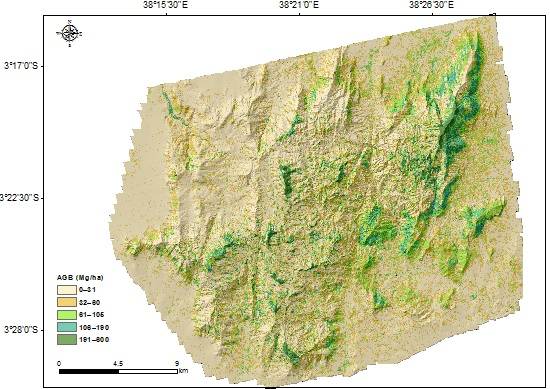
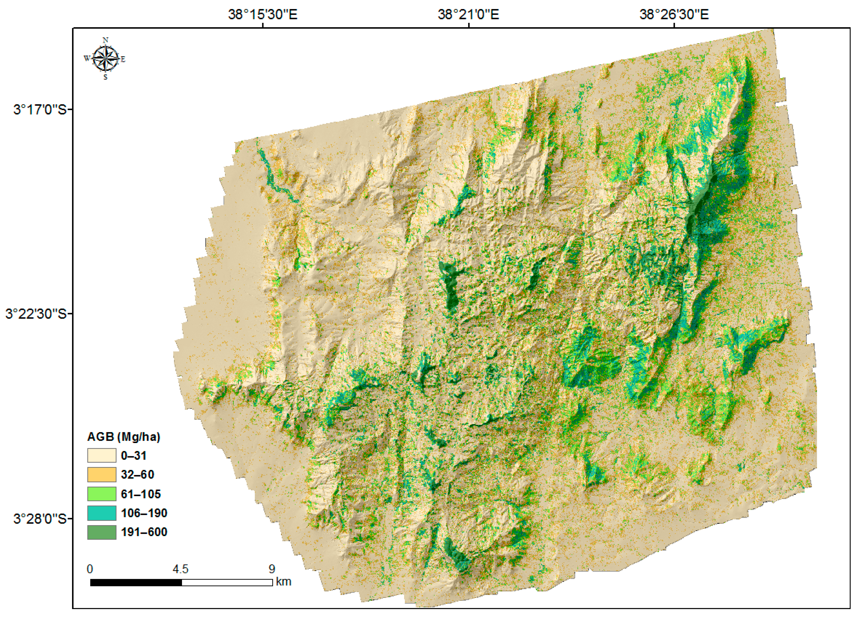
The AGB map predicted at 30 m × 30 m resolution is shown in Figure 3. The largest values were concentrated on montane forest patches in the hills and slopes with northeast and southeast aspects. In general, the AGB density decreases towards the lower elevations. Furthermore, lower densities (less than 31 Mg ha−1) are observed in the northwestern part of the area, which is in the rain-shadow of the hills. Some hilltops, for example in Yale and Ngangao, are without tree cover. In the foothills and lowlands, AGB densities are low and less variable compared with the hills, particularly in the northeast and southeast parts of the area. In the lowlands, larger AGB is concentrated in riverine areas, as those provide the consistent wetness necessary for trees.
3.2. Determinants of Aboveground Biomass
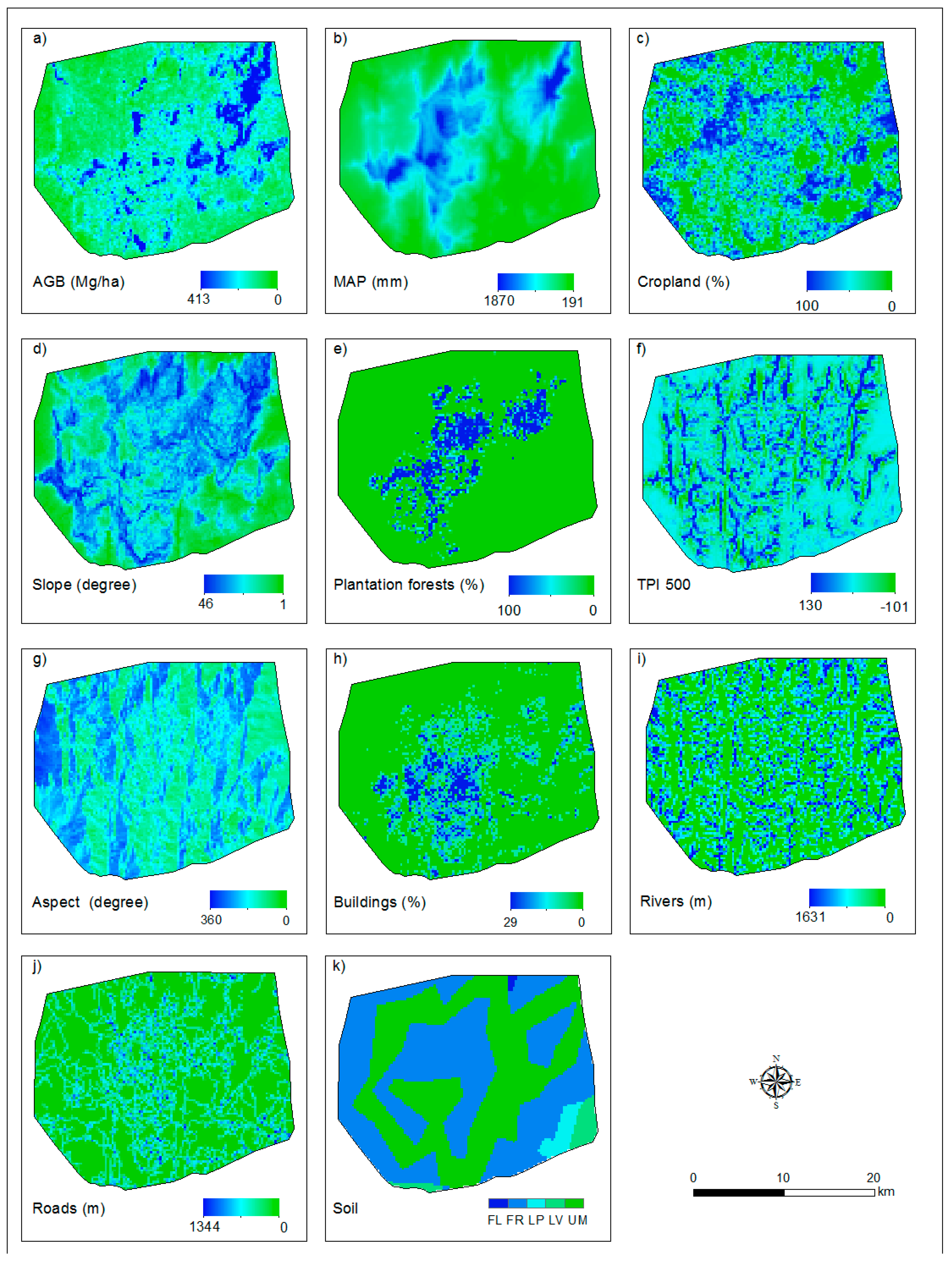
The AGB map and all of the explanatory variables used to explain the spatial distribution of AGB in the Afromontane landscape are shown in Figure A3. Plantation forests are limited in the northeast and southwest regions, which could be due to the distribution of precipitation in the region. LULC variables, for example buildings, are spatially concentrated, and croplands are really sparsely distributed (Figure A3).
The total explained deviance (cross-validated D2) of the BRT model was 72.7%. Figure 4 shows the relative importance and partial dependence plot for each explanatory variable. The most influential variables were MAP (37.6%), cropland (16.9%) and slope (15.3%). Only 5.9% of the total deviance was explained by rivers, roads and soil type.
According to the partial dependence plots, AGB increases rapidly with increasing precipitation after approximately 1240 mm, which corresponds to elevations above 1350 m. Cropland and slope also play a role in AGB distribution, especially at the lower cropland coverage and the steeper slope (<37 degrees).
The effect of the plantation as predictor variables is observed especially at the lower plantation coverage (i.e., below 65%), and above that, it is constant. Plantation forests were available on small patches, and only a few areas were completely covered. The relative strength of the contribution of TPI500 is high especially at the beginning and end of the range. At the landscape scale (TPI500), high AGB was found both in the upper and lower slope. Aspect clearly shows that AGB is more concentrated in northeast and southeast slopes with decreasing AGB on the leeward side. Furthermore, areas with fewer buildings contain more AGB.
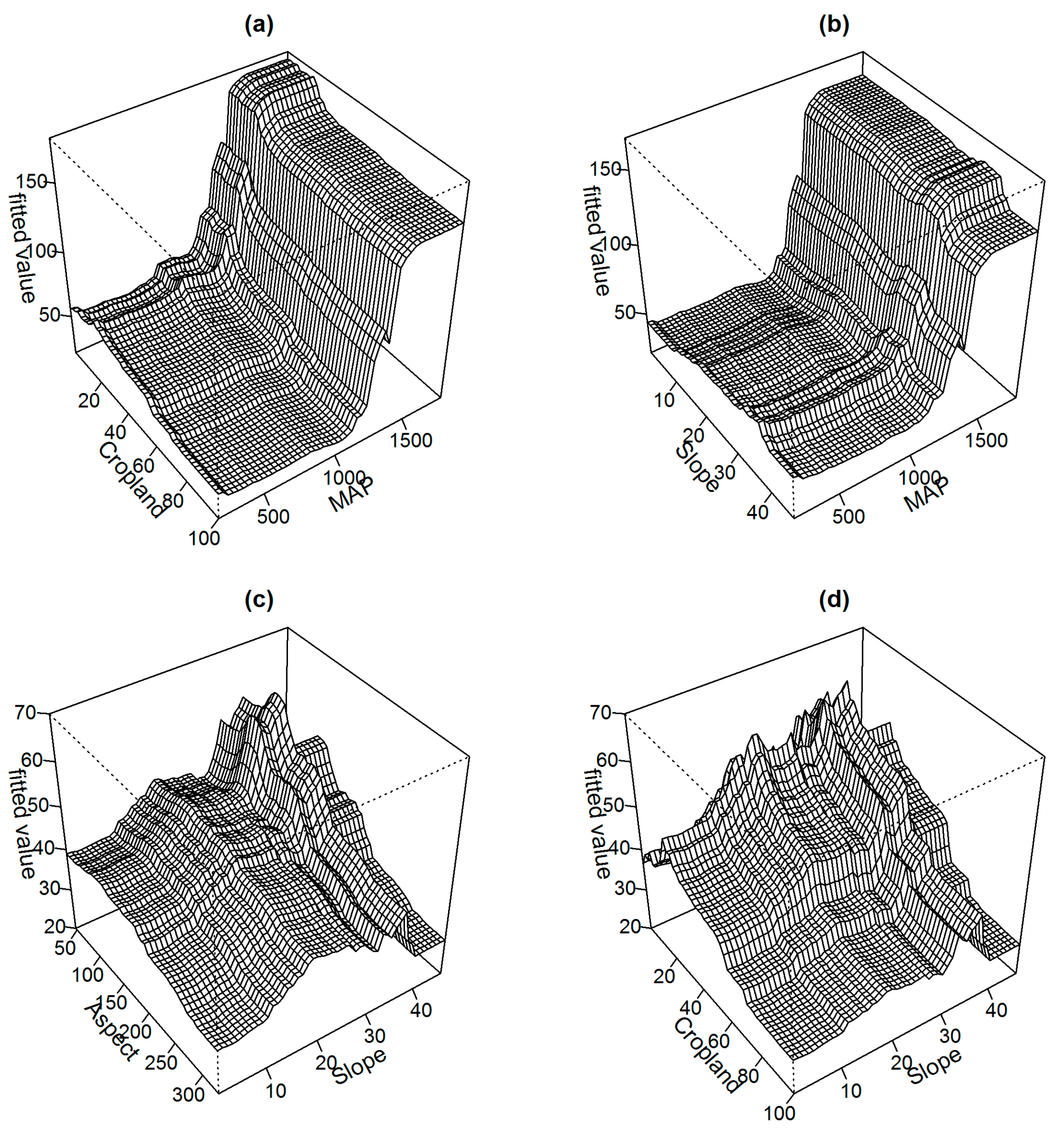
Figure 5 displays two-variable partial dependence plots on some of the most influential variables. Interaction effects of varying degree are presented among these variable pairs. The strongest interactions in the final model were observed between MAP and cropland (Figure 5a), and MAP and slope (Figure 5b). Cropland and slope have important effects on the predicted spatial distribution of AGB when MAP is at the highest and cropland and slope are at the lowest fraction (below 20) and below 37 degrees, respectively. When MAP is less than approximately 1250 mm, cropland and slope have low impacts on AGB. Additionally, the steep slope (up to 37 degrees) in the northeast aspect (Figure 5c) and regions with low cropland fraction (Figure 5d) contain high AGB. However, comparatively less AGB is present in the steepest slope.
4. Discussion
4.1. ALS-Based Aboveground Biomass Map
Using a combination of field plots and ALS metrics, a wall-to-wall high-resolution AGB map was made for the Taita Hills. The AGB model had an R2 of 0.88 and an RMSE of 52.9 Mg⋅ha−1 (43%). Some of the previous studies in the tropics have achieved better model fits and accuracies [10,12,16,63]. However, a larger plot size has usually been used, which reduces the error [18]. Furthermore, the heterogeneous land cover could explain the worse accuracy, but a single model for the whole area was considered appropriate here as systematic over- or under-estimation was not observed. Therefore, averaging AGB estimates to 250 m × 250 m resolution for modelling is likely to improve accuracy considerably [6]. The final model was based on percentile height (H.p25) and canopy cover (CC.all.first). The variables are in line with the previous studies in Africa, which have used, for example, mean canopy height, height percentiles and canopy density for modelling [6,10,11,12]. Both modelling accuracy and explanatory variables are similar to the model used for the hills in the study by [15], who developed separate models for hills and lowlands using different ALS data.
Although the general patterns of AGB are very similar, the current map is an improvement over an earlier aboveground carbon map for the Taita Hills [15]. The authors in [15] generated their map for analyzing the effect of the land cover change on carbon stocks using a satellite image-based land cover map and land cover type-specific mean carbon density values. However, the continuous AGB estimates are important as AGB depends on many variables, also within land cover classes (see Section 4.2). If converted to carbon, the new map had slightly larger mean carbon densities for montane forests (94.9 Mg⋅C⋅ha−1), exotic plantation forests (36.0 Mg⋅C⋅ha−1) and woodland (27.1 Mg⋅C⋅ha−1) in comparison to [15], who reported mean values of 89.5 Mg⋅C⋅ha−1, 29.4 Mg⋅C⋅ha−1 and 16.8 Mg⋅C⋅ha−1, respectively.
Uncertainties in the ALS-based mapping could be decreased by using species-specific allometric equations [37]. Due to the absence of local wood density data and species-level allometric equations, beside genera Acacia and Eucalyptus, we used [40] for the rest of the species. Therefore, future studies should attempt to contribute to filling this gap. Furthermore, stems having D < 10 cm were not sampled in this study as they usually contribute only little to the aboveground carbon in mature African tropical forests [20,64]. However, in a boreal forest, The author of [65] showed that a minimum DBH of 3 cm produced better AGB modelling results than 10 cm for the young forests, although improvement was small for the mature forests. Therefore, having a smaller DBH limit could improve modelling accuracy slightly in the areas with abundant small trees and shrubs. Additionally, the slope can bias ALS height percentiles [66], which were used in the final AGB model. This could increase AGB predictions in the steep slopes with an effect on the BRT analysis (Section 4.2), and future studies should consider applying a slope correction [67] before computing ALS height metrics. Nonetheless, there was no sign of systematic overestimation in the steep slopes when assessing the model residuals against the slope.
4.2. Determinants of Aboveground Biomass Distribution
AGB distribution in the Taita Hills is driven by the quantity and spatial distribution of precipitation. Precipitation is uneven due to the orographic rain pattern causing the eastern slopes and eastern parts of the hills to receive more precipitation than the leeward side in the western region, which is suffering from high water stress. AGB was the greatest at mid-altitude hills where MAP is high in comparison with the lowlands. The authors of [21] observed that precipitation explained 39% of the variation in LAI, and LAI increased significantly with increasing MAP in woody biomes. The bimodal rainfall pattern in the study area provides precipitation for more than half a year. In this study, precipitation explained 37.6% of AGB variation. The authors of [68] observed that AGB in African tropical forests shows a positive relationship with rainfall in the driest nine months and is negative for the wettest three months of the year. Low AGB in the lowlands could be due to higher air temperature, which results in higher respiration, and low precipitation in the lowlands could limit photosynthesis.
Both precipitation and temperature are closely related to elevation. We removed elevation and MAT from the analysis as they strongly correlated with MAP. The authors of [6] observed that elevation and the fraction of photosynthetic vegetation cover together accounted for 27–67% of the spatial variation in aboveground carbon density in areas in the north and south aspects of Madagascar. The authors of [20] revealed that AGB was the greatest in gentle slope and mid-elevation, which explained 63.7% of the variation in aboveground carbon in the Eastern Arc Mountains, especially Tanzania. The authors of [16] highlighted the fact that increasing elevation corresponds to a 53–84% decrease in AGB levels depending on substrate age class. Normally, at higher elevations, growth can be limited by water shortage and reduced temperature [20,69]. However, in tropical montane cloud forests, high atmospheric-humidity levels are sustained due to frequent cloud cover and fog [69].
Furthermore, greater AGB was found in areas with smaller cropland fraction and on the relatively steep slope, compared with valleys and ridges. Croplands, if present in the mid-altitude, are concentrated on the northern and southwestern slopes, for example around Vuria and Ngangao. There is an increasing trend in croplands at the expense of thickets and shrublands in the lowlands. The amount of precipitation is low in the lowlands, which is directly linked with productivity. In the hills above 1220 m a.s.l., croplands are converted to shrublands and woodlands, due to the growing number of trees in the farms due to agroforestry and government policies [15]. Besides that, cropland in hills has less economic returns from cash crop and high labor demand. This pattern is also observed here as even though the cropland fraction in the area is more than 50%, there is still some AGB (<120 Mg⋅ha−1). Steeper slopes have less cropland as they are not suitable for agriculture due to soil loss during heavy rainfall. The slope was the most important control in tropical landscapes in Costa Rica [19]. Convexity, elevation and slope were significantly related to AGB in subtropical broad-leaved forests of Taiwan [70]. The results are in line with [19] and [70], as slope also explained more of the variation in AGB in the Afromontane landscape mosaic. In this study, larger AGBs are limited to steep slopes (<37 degrees), compared with shallow and steepest slope in [20] and [71]. The steepest slopes and hilltops are covered by bare rocks, and they do not have enough nutrients and soil to hold high biomass forests. For instance, part of the hilltops in Ngangao are covered by Erica mannii and the top of Vuria by short elfin forests. The forest on the hilltops is also reserved for conservation under the Kenya Forest Service [72] and recognized as sacred forests [73].
Plantation of trees on former agriculture lands substantially increases biomass accumulation during the first few years of forest recovery in the restored tropical forest in Costa Rica [74]. In addition to the small and fragmented indigenous forest patches, the Taita Hills host plantations of exotic tree species, such as Cupressus lusitanica, Eucalyptus spp., Grevillea robusta and Pinus spp. [24], which explained 8.3% of the AGB variation. Forests found on a steep slope at higher altitudes were less likely to be deforested and less accessible to transport forest materials, while they were more likely to contain the tallest trees harboring the highest AGB. However, the height of trees is low in the upper montane forest, like in Vuria, which could be due to the frequent occurrence of low cloud, the possibility of mechanical damage due to the wind and low radiation (persistence cloud) [69].
Except for plantation and cropland, other land use and land cover variables were found to be relatively insensitive to the spatial distribution of AGB, for example road and rivers. Built-up areas are sparsely distributed and have less impact on AGB. The local people practice agroforestry in the hills in order to preserve the soil, its nutrients and provide shade from trees. There is a low population density in the drier northwestern part of the study area. The authors of [75] showed the dependency of dense population with precipitation in the Taita Hills. In rural Africa, dense populations are linked to croplands with low biomass compared with forests. The authors of [18] observed that for upland tropical rain forest landscapes, AGB was relatively insensitive to soil type and topography. The influence of soil was among the lowest also in this study.
Previous studies have analyzed the relationship between ALS-based AGB and biotic and abiotic explanatory variables from the plot to the landscape level [6,18,19]. The relationship between the predictors and response variables differs between biomes and changes over spatial scales and through time [60]. The fitted functions are not supposed to be applied to another area as the objective of BRT analysis was to help with understanding the controlling factors of AGB, but not making a predictive model for AGB. Although the regression methods were different, explanatory variables with higher spatial resolution (1 ha) explained 67% of the spatial variation in aboveground carbon density in [6]. Additional research is needed to compare the explained deviance using the same regression techniques and explanatory variables at different spatial resolutions. Furthermore, the model could be further improved by including forest stand characteristics, for example stand age or disturbance history.
5. Conclusions
The Taita Hills comprise a human-dominated landscape with heterogeneous land cover and forest being limited to small patches typically far from the main areas of human settlement. In this study, field estimates of AGB were used for mapping AGB using ALS metrics to construct a wall-to-wall map for the Taita Hills area. ALS metrics representing the height of the canopy and canopy cover (i.e., volume of the canopy) predict AGB with the highest accuracy. AGB is concentrated in native moist evergreen montane forests, which are located in the windward side in the north and southeast aspects of the Taita Hills in higher elevations receiving more rainfall. The high biomass areas are also located on hilltops and steep slopes, as they are too cumbersome to take into agricultural practice. This study revealed the influence of climate, land use and topography in shaping the spatial patterns in AGB in a heterogeneous landscape. Using the coverage of the AGB map and various explanatory variables, it was possible to capture the spatial variation in AGB throughout the highly complex region and a large altitudinal gradient. Hence, the results provide novel insights into the cross-scale nature of determinants of AGB, in a region where multiple factors may interact non-linearly in defining landscape-level AGB.
Acknowledgments
We would like to thank the Building Biocarbon and Rural Development in West Africa (BIODEV) project funded by the Ministry of Foreign Affairs of Finland, the Integrated land cover-climate-ecosystem process study for water management in the East African highlands (TAITAWATER) project funded by the Academy of Finland and the Faculty of Science of the University of Helsinki for making ALS data available. In addition, this study is a result of the project: Remote sensing of water harvesting and carbon sequestration by forests in the Taita Hills, Kenya, funded by the Finnish Culture Foundation. The Taita Research Station of the University of Helsinki in Kenya is gratefully acknowledged for logistical support and Darius Kimuzi, Benson Mwakachola Lombo, Jessica Broas, Jesse Hietanen, Elisa Schäfer for field assistance. Mr. Adhikari is currently funded by the Doctoral Programme in Atmospheric Sciences (ATM-DP, University of Helsinki) and was supported by Geoinformatics in Monitoring and Modelling Environment Change (GIMMEC) during the initial period. Research Permit NCST/RCD/17/012/33 for the Taita Research Station from the National Council for Science and Technology of Kenya is gratefully acknowledged. Two anonymous reviewers and the Journal Editor are thanked for useful insights and comments that helped improve this work.
Author Contributions
Hari Adhikari, Janne Heiskanen and Mika Siljander conceived of and designed the experiments. Hari Adhikari performed the experiments. Hari Adhikari and Janne Heiskanen analyzed the data. Hari Adhikari, Janne Heiskanen, Vuokko Heikinheimo and Petri Pellikka contributed materials/analysis tools. Hari Adhikari wrote the paper. Janne Heiskanen, Eduardo Maeda, Vuokko Heikinheimo, Petri Pellikka and Mika Siljander commented on the manuscript.
Conflicts of Interest
The authors declare no conflict of interest.
Appendix A
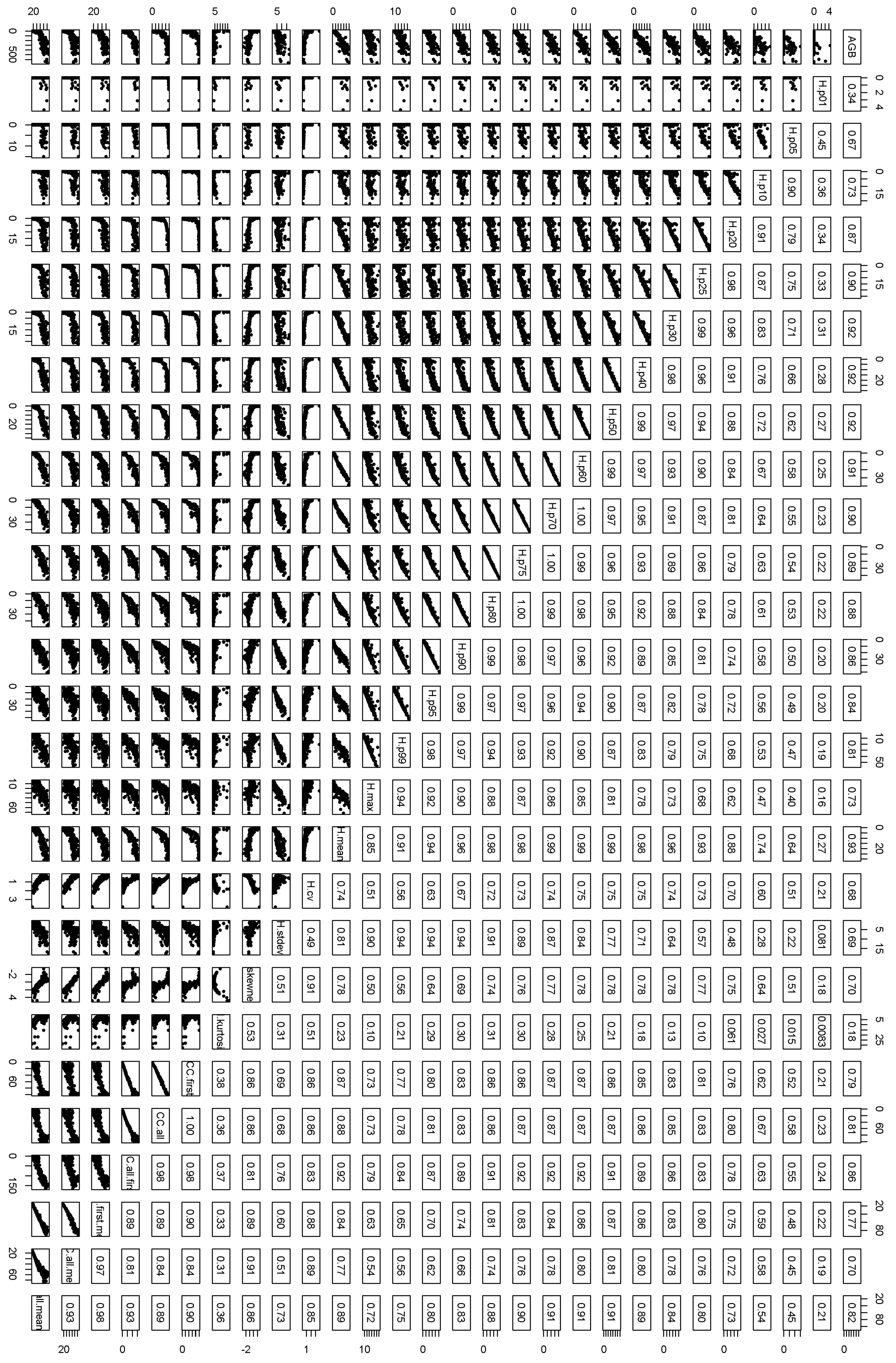
Figure A1.
Pearson correlation between the ALS metrics and their scatter plots. Variables name in the diagonal follow the same pattern as in Table 3 (Metric column).
Figure A1.
Pearson correlation between the ALS metrics and their scatter plots. Variables name in the diagonal follow the same pattern as in Table 3 (Metric column).

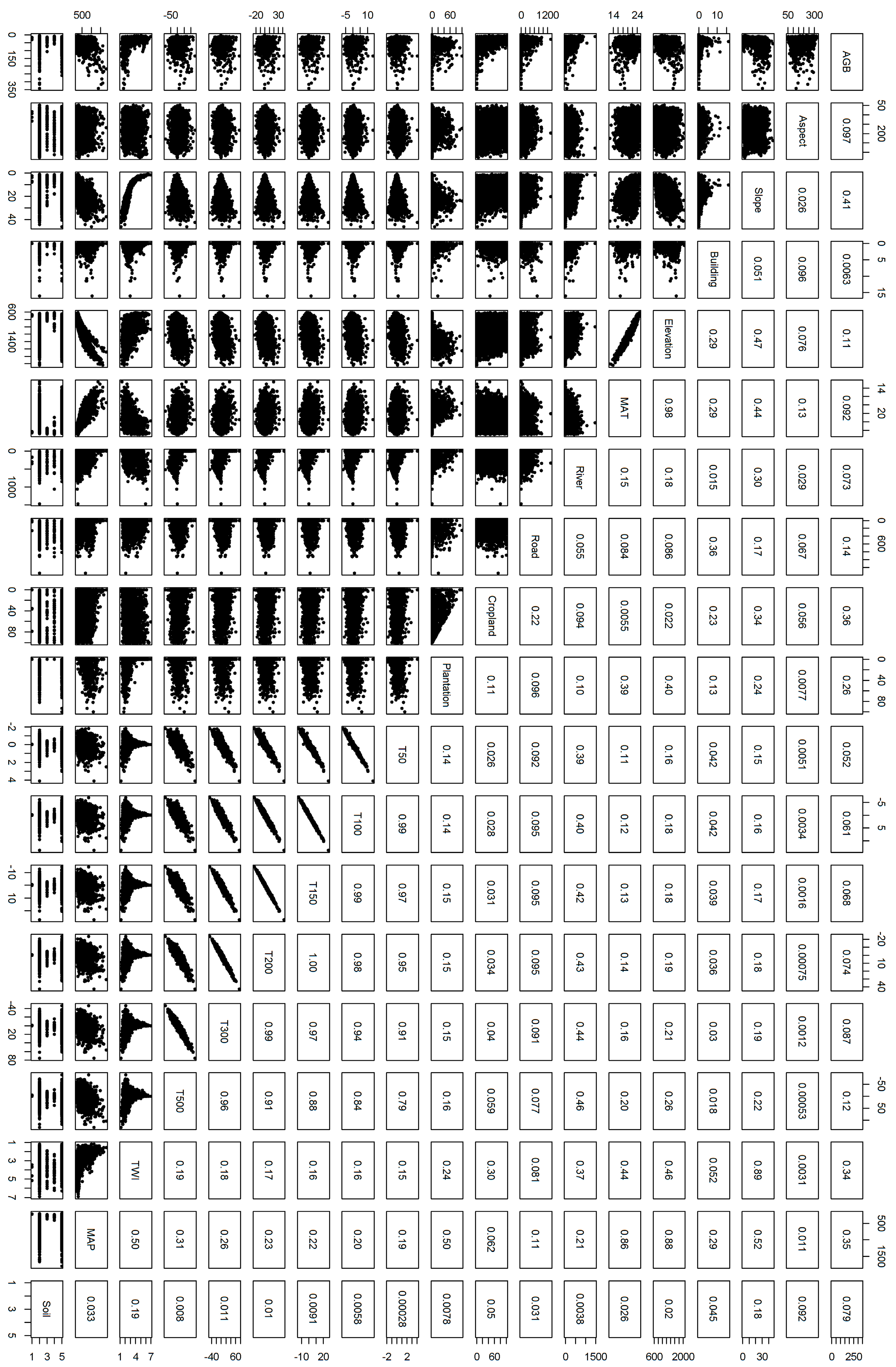
Figure A2.
Pearson correlation between the variables and their scatter plots.

Figure A3.
ALS-based aboveground biomass (AGB) map (a) and (b–k) explanatory variables at 250-m resolution. MAP is the mean annual precipitation, and TPI 500 is the topographic position index with a 500-m radius. Panels (i) and (j) refer to the distance of the river and roads in the given pixel (i.e., 250 m × 250 m). See Table 4 for description of the variables.
References
- Lovett, J.C.; Wasser, S.K. Biogeography and Ecology of the Rainforests of Eastern Africa; Cambridge University Press: Cambridge, UK, 1993. [Google Scholar]
- Ioki, K.; Tsuyuki, S.; Hirata, Y.; Phua, M.-H.; Wong, W.V.C.; Ling, Z.-Y.; Saito, H.; Takao, G. Estimating above-ground biomass of tropical rainforest of different degradation levels in Northern Borneo using airborne LiDAR. Forest Ecol. Manag. 2014, 328, 335–341. [Google Scholar] [CrossRef]
- Pellikka, P.K.E.; Clark, B.J.F.; Gosa, A.G.; Himberg, N.; Hurskainen, P.; Maeda, E.; Mwang’ombe, J.; Omoro, L.M.A.; Siljander, M. Chapter 13—Agricultural expansion and its consequences in the Taita Hills, Kenya. In Developments in Earth Surface Processes; Paolo Paron, D.O.O., Christian Thine, O., Eds.; Elsevier: Amsterdam, The Netherlands, 2013. [Google Scholar]
- Pfeifer, M.; Platts, P.J.; Burgess, N.D.; Swetnam, R.D.; Willcock, S.; Lewis, S.L.; Marchant, R. Land use change and carbon fluxes in East Africa quantified using earth observation data and field measurements. Environ. Conserv. 2012, 40, 241–252. [Google Scholar] [CrossRef]
- United Nations Framework Convention on Climate Change. Available online: http://unfccc.int/meetings/bali_dec_2007/meeting/6319.php (accessed on 11 August 2017).
- Asner, G.P.; Clark, J.K.; Mascaro, J.; Vaudry, R.; Chadwick, K.D.; Vieilledent, G.; Rasamoelina, M.; Balaji, A.; Kennedy-Bowdoin, T.; Maatoug, L.; et al. Human and environmental controls over aboveground carbon storage in Madagascar. Carbon Balance Manag. 2012, 7, 2. [Google Scholar] [CrossRef] [PubMed] [Green Version]
- Lu, D. The potential and challenge of remote sensing-based biomass estimation. Int. J. Remote Sens. 2006, 27, 1297–1328. [Google Scholar] [CrossRef]
- Zolkos, S.G.; Goetz, S.J.; Dubayah, R. A meta-analysis of terrestrial aboveground biomass estimation using LiDAR remote sensing. Remote Sens. Environ. 2013, 128, 289–298. [Google Scholar] [CrossRef]
- Singh, K.K.; Chen, G.; McCarter, J.B.; Meentemeyer, R.K. Effects of LiDAR point density and landscape context on estimates of urban forest biomass. ISPRS J. Photogramm. Remote Sens. 2015, 101, 310–322. [Google Scholar] [CrossRef]
- Vaglio Laurin, G.; Chen, Q.; Lindsell, J.A.; Coomes, D.A.; Frate, F.D.; Guerriero, L.; Pirotti, F.; Valentini, R. Above ground biomass estimation in an African tropical forest with LiDAR and hyperspectral data. ISPRS J. Photogramm. Remote Sens. 2014, 89, 49–58. [Google Scholar] [CrossRef]
- Hansen, E.H.; Gobakken, T.; Bollandsas, O.M.; Zahabu, E.; Naesset, E. Modeling aboveground biomass in dense tropical submontane rainforest using airborne laser scanner data. Remote Sens. 2015, 7, 788–807. [Google Scholar] [CrossRef] [Green Version]
- Chen, Q.; Vaglio Laurin, G.; Valentini, R. Uncertainty of remotely sensed aboveground biomass over an African tropical forest: Propagating errors from trees to plots to pixels. Remote Sens. Environ. 2015, 160, 134–143. [Google Scholar] [CrossRef]
- Vaglio Laurin, G.; Puletti, N.; Chen, Q.; Corona, P.; Papale, D.; Valentini, R. Above ground biomass and tree species richness estimation with airborne LiDAR in tropical Ghana forests. Int. J. Appl. Earth Obs. 2016, 52, 371–379. [Google Scholar] [CrossRef]
- Zomer, R.J.; Neufeldt, H.; Xu, J.; Ahrends, A.; Bossio, D.; Trabucco, A.; van Noordwijk, M.; Wang, M. Global tree cover and biomass carbon on agricultural land: The contribution of agroforestry to global and national carbon budgets. Sci. Rep. 2016, 6, 29987. [Google Scholar] [CrossRef] [PubMed]
- Pellikka, P.K.E.; Heikinheimo, V.; Hietanen, J.; Schäfer, E.; Siljander, M.; Heiskanen, J. Assessment of the impact of land cover change on aboveground carbon stocks using airborne LiDAR data and satellite imagery in Afromontane landscape in Kenya. 2017; Submitted. [Google Scholar]
- Asner, G.P.; Hughes, R.F.; Varga, T.A.; Knapp, D.E.; Kennedy-Bowdoin, T. Environmental and biotic controls over aboveground biomass throughout a tropical rain forest. Ecosystems 2009, 12, 261–278. [Google Scholar] [CrossRef]
- Singh, K.K.; Bianchetti, R.A.; Chen, G.; Meentemeyer, R.K. Assessing effect of dominant land-cover types and pattern on urban forest biomass estimated using LiDAR metrics. Urban Ecosyst. 2017, 20, 265–275. [Google Scholar] [CrossRef]
- Clark, D.B.; Clark, D.A. Landscape-scale variation in forest structure and biomass in a tropical rain forest. Forest Ecol. Manag. 2000, 137, 185–198. [Google Scholar] [CrossRef]
- Taylor, P.; Asner, G.; Dahlin, K.; Anderson, C.; Knapp, D.; Martin, R.; Mascaro, J.; Chazdon, R.; Cole, R.; Wanek, W.; et al. Landscape-scale controls on aboveground forest carbon stocks on the Osa Peninsula, Costa Rica. PLoS ONE 2015, 10, e0126748. [Google Scholar] [CrossRef] [PubMed]
- Marshall, A.R.; Willcock, S.; Platts, P.J.; Lovett, J.C.; Balmford, A.; Burgess, N.D.; Latham, J.E.; Munishi, P.K.T.; Salter, R.; Shirima, D.D.; et al. Measuring and modelling above-ground carbon and tree allometry along a tropical elevation gradient. Biol. Conserv. 2012, 154, 20–33. [Google Scholar] [CrossRef]
- Pfeifer, M.; Gonsamo, A.; Disney, M.; Pellikka, P.; Marchant, R. Leaf area index for biomes of the Eastern Arc Mountains: Landsat and spot observations along precipitation and altitude gradients. Remote Sens. Environ. 2012, 118, 103–115. [Google Scholar] [CrossRef]
- Commission on Revenue Allocation. Available online: http://www.crakenya.org/ (accessed on 11 August 2017).
- Erdogan, H.E.; Pellikka, P.K.E.; Clark, B. Modelling the impact of land-cover change on potential soil loss in the Taita Hills, Kenya, between 1987 and 2003 using remote-sensing and geospatial data. Int. J. Remote Sens. 2011, 32, 5919–5945. [Google Scholar] [CrossRef]
- Pellikka, P.K.E.; Lötjönen, M.; Siljander, M.; Lens, L. Airborne remote sensing of spatiotemporal change (1955–2004) in indigenous and exotic forest cover in the Taita Hills, Kenya. Int. J. Appl. Earth Obs. 2009, 11, 221–232. [Google Scholar] [CrossRef]
- Aerts, R.; Thijs, K.W.; Lehouck, V.; Beentje, H.; Bytebier, B.; Matthysen, E.; Gulinck, H.; Lens, L.; Muys, B. Woody plant communities of isolated afromontane cloud forests in Taita Hills, Kenya. Plant Ecol. 2011, 212, 639–649. [Google Scholar] [CrossRef] [Green Version]
- Stam, Å.; Enroth, J.; Malombe, I.; Pellikka, P.; Rikkinen, J. Experimental transplants reveal strong environmental effects on the growth on non-vascular epiphytes in Afromontane forests. Biotropica 2017. in print. [Google Scholar] [CrossRef]
- Enroth, J.; Nyqvist, P.; Malombe, I.; Pellikka, P.; Rikkinen, J. Additions to the moss flora of the Taita Hills and mount Kasigau, Kenya. Polish Bot. J. 2013, 58, 495. [Google Scholar] [CrossRef]
- Thijs, K.W.; Aerts, R.; Musila, W.; Siljander, M.; Matthysen, E.; Lens, L.; Pellikka, P.; Gulinck, H.; Muys, B. Potential tree species extinction, colonization and recruitment in Afromontane forest relicts. Basic Appl. Ecol. 2014, 15, 288–296. [Google Scholar] [CrossRef] [Green Version]
- Thijs, K.W.; Aerts, R.; van de Moortele, P.; Aben, J.; Musila, W.; Pellikka, P.; Gulinck, H.; Muys, B. Trees in a human-modified tropical landscape: Species and trait composition and potential ecosystem services. Landscape Urban. Plan. 2015, 144, 49–58. [Google Scholar] [CrossRef]
- European Spatial Agency. Sentinel-2 User Handbook. ESA Standard Document. Available online: https://sentinel.esa.int/documents/247904/685211/Sentinel-2_User_Handbook (accessed on 24 July 2015).
- Heiskanen, J.; Korhonen, L.; Hietanen, J.; Pellikka, P.K.E. Use of airborne LiDAR for estimating canopy gap fraction and leaf area index of tropical montane forests. Int. J. Remote Sens. 2015, 36, 2569–2583. [Google Scholar] [CrossRef]
- Piiroinen, R.; Heiskanen, J.; Mõttus, M.; Pellikka, P. Classification of crops across heterogeneous agricultural landscape in Kenya using Aisaeagle imaging spectroscopy data. Int. J. Appl. Earth Obs. 2015, 39, 1–8. [Google Scholar] [CrossRef]
- Curtis, R.O. Height-diameter and height-diameter-age equations for second-growth douglas-fir. Forest Sci. 1967, 13, 365–375. [Google Scholar]
- Valbuena, R.; Heiskanen, J.; Aynekulu, E.; Pitkänen, S.; Packalen, P. Sensitivity of above-ground biomass estimates to height-diameter modelling in mixed-species West African woodlands. PLoS ONE 2016, 11, e0158198. [Google Scholar] [CrossRef] [PubMed]
- R Core Team. Nlme: Linear and Nonlinear Mixed Effects Models. R Package Version 3.1–118. Available online: http://CRAN.R-project.org/package=nlme (accessed on 6 February 2017).
- R Core Team. R: A Language and Environment for Statistical Computing. Available online: http://www.gbif.org/resource/81287 (accessed on 11 August 2017).
- Henry, M.; Picard, N.; Trotta, C.; Manlay, R.; Valentini, R.; Bernoux, M.; Saint-André, L. Estimating tree biomass of sub-Saharan African forests: A review of available allometric equations. Silva Fenn. 2011, 45, 477–569. [Google Scholar] [CrossRef]
- Paul, K.I.; Roxburgh, S.H.; England, J.R.; Ritson, P.; Hobbs, T.; Brooksbank, K.; John Raison, R.; Larmour, J.S.; Murphy, S.; Norris, J.; et al. Development and testing of allometric equations for estimating above-ground biomass of mixed-species environmental plantings. Forest Ecol. Manag. 2013, 310, 483–494. [Google Scholar] [CrossRef]
- Frangi, J.L.; Lugo, A.E. Ecosystem dynamics of a subtropical floodplain forest. Ecol. Monogr. 1985, 55, 351–369. [Google Scholar] [CrossRef]
- Chave, J.; Réjou-Méchain, M.; Búrquez, A.; Chidumayo, E.; Colgan, M.S.; Delitti, W.B.C.; Duque, A.; Eid, T.; Fearnside, P.M.; Goodman, R.C.; et al. Improved allometric models to estimate the aboveground biomass of tropical trees. Glob. Chang. Biol. 2014, 20, 3177–3190. [Google Scholar] [CrossRef] [PubMed]
- ICRAF. World Agroforestry Center Wood Density Database. Available online: https://www.worldagroforestry.org/output/wood-density-database (accessed on 2 February 2016).
- Data from: Towards A Worldwide Wood Economics Spectrum. Available online: http://datadryad.org/resource/doi:10.5061/dryad.234 (accessed on 4 February 2009).
- Cao, L.; Coops, N.C.; Innes, J.L.; Sheppard, S.R.J.; Fu, L.; Ruan, H.; She, G. Estimation of forest biomass dynamics in subtropical forests using multi-temporal airborne LiDAR data. Remote Sens. Environ. 2016, 178, 158–171. [Google Scholar] [CrossRef]
- McGaughey, R.J. Fusion/LDV: Software for LiDAR Data Analysis and Visualization; US Department of Agriculture, Forest Service, Pacific Northwest Research Station: Seattle, WA, USA, 2016.
- Asner, G.P.; Mascaro, J. Mapping tropical forest carbon: Calibrating plot estimates to a simple LiDAR metric. Remote Sens. Environ. 2014, 140, 614–624. [Google Scholar] [CrossRef]
- Bouvier, M.; Durrieu, S.; Fournier, R.A.; Renaud, J.-P. Generalizing predictive models of forest inventory attributes using an area-based approach with airborne LiDAR data. Remote Sens. Environ. 2015, 156, 322–334. [Google Scholar] [CrossRef]
- Package ‘Leaps’. Available online: https://cran.r-project.org/web/packages/leaps/leaps.pdf (accessed on 10 January 2017).
- Zuur, A.F.; Ieno, E.N.; Elphick, C.S. A protocol for data exploration to avoid common statistical problems. Methods Ecol. Evol. 2010, 1, 3–14. [Google Scholar] [CrossRef]
- Weiss, A. Topographic Position and Landforms Analysis. Available online: http://www.jennessent.com/downloads/TPI-poster-TNC_18x22.pdf (accessed on 11 August 2017).
- Guisan, A.; Weiss, S.B.; Weiss, A.D. GLM versus CCA spatial modeling of plant species distribution. Plant Ecol. 1999, 143, 107–122. [Google Scholar] [CrossRef]
- Böhner, J.; Köthe, R.; Conrad, O.; Gross, J.; Ringeler, A.; Selige, T. Soil regionalisation by means of terrain analysis and process parameterisation. In Soil Classification; The European Soil Bureau, Joint Research Centre: Ispra, Italy, 2002. [Google Scholar]
- Costa-Cabral, M.C.; Burges, S.J. Digital elevation model networks (DEMON): A model of flow over hillslopes for computation of contributing and dispersal areas. Water Resour. Res. 1994, 30, 1681–1692. [Google Scholar] [CrossRef]
- Soil Atlas of Africa and Its Associated Soil Map (Data). Available online: http://esdac.jrc.ec.europa.eu/content/soil-map-soil-atlas-africa (accessed on 21 June 2017).
- Virtanen, E. Fine-Resolution Climate Grids for Species Studies in Data-Poor Regions. Available online: https://helda.helsinki.fi/handle/10138/156514 (accessed on 11 September 2015).
- Hutchinson, M.F. The application of thin plate splines to continent-wide data assimilation. BMRC Res. Rep. 1991, 27, 104–113. [Google Scholar]
- Heikinheimo, V. Impact of Land Change on Aboveground Carbon Stocks in the Taita Hills, Kenya. Master’s Thesis, University of Helsinki, Helsinki, Finland, 25 May 2015. [Google Scholar]
- ESRI. Redlands, CA: 1999–2015. Available online: http://www.esri.com/data/basemaps (accessed on 21 June 2017).
- Elith, J.; Leathwick, J.R.; Hastie, T. A working guide to boosted regression trees. J. Anim. Ecol. 2008, 77, 802–813. [Google Scholar] [CrossRef] [PubMed]
- Riihimäki, H.; Heiskanen, J.; Luoto, M. The effect of topography on arctic-alpine aboveground biomass and ndvi patterns. Int. J. Appl. Earth Obs. 2017, 56, 44–53. [Google Scholar] [CrossRef]
- Dormann, C.F.; Elith, J.; Bacher, S.; Buchmann, C.; Carl, G.; Carré, G.; Marquéz, J.R.G.; Gruber, B.; Lafourcade, B.; Leitão, P.J.; et al. Collinearity: A review of methods to deal with it and a simulation study evaluating their performance. Ecography 2013, 36, 27–46. [Google Scholar] [CrossRef]
- Hijmans, R.J.; Phillips, S.J.; Leathwick, J.; Elith, J. Package ‘dismo’. Available online: http://www12.frugalware.org/mirrors/cran.r-project.org/web/packages/dismo/dismo.pdf (accessed on 9 January 2017).
- Gregoire, T.G.; Lin, Q.F.; Boudreau, J.; Nelson, R. Regression estimation following the square root transformation of the response. Forest Sci. 2008, 54, 597–606. [Google Scholar]
- Mascaro, J.; Detto, M.; Asner, G.P.; Muller-Landau, H.C. Evaluating uncertainty in mapping forest carbon with airborne LiDAR. Remote Sens. Environ. 2011, 115, 3770–3774. [Google Scholar] [CrossRef]
- Chave, J.; Condit, R.; Muller-Landau, H.C.; Thomas, S.C.; Ashton, P.S.; Bunyavejchewin, S.; Co, L.L.; Dattaraja, H.S.; Davies, S.J.; Esufali, S.; et al. Assessing evidence for a pervasive alteration in tropical tree communities. PLoS Biol. 2008, 6, e45. [Google Scholar] [CrossRef] [PubMed] [Green Version]
- Keränen, J.; Peuhkurinen, J.; Packalen, P.; Maltamo, M. Effect of minimum diameter at breast height and standing dead wood field measurements on the accuracy of als-based forest inventory. Can. J. Forest Res. 2015, 45, 1280–1288. [Google Scholar] [CrossRef]
- Breidenbach, J.; Koch, B.; Kändler, G.; Kleusberg, A. Quantifying the influence of slope, aspect, crown shape and stem density on the estimation of tree height at plot level using LiDAR and insar data. Int. J. Remote Sens. 2008, 29, 1511–1536. [Google Scholar] [CrossRef]
- Duan, Z.; Zhao, D.; Zeng, Y.; Zhao, Y.; Wu, B.; Zhu, J. Assessing and correcting topographic effects on forest canopy height retrieval using airborne LiDAR data. Sensors 2015, 15, 12133. [Google Scholar] [CrossRef] [PubMed]
- Lewis, S.L.; Sonké, B.; Sunderland, T.; Begne, S.K.; Lopez-Gonzalez, G.; van der Heijden, G.M.F.; Phillips, O.L.; Affum-Baffoe, K.; Baker, T.R.; Banin, L.; et al. Above-ground biomass and structure of 260 African tropical forests. Philos. Trans. R. Soc. B 2013, 368. [Google Scholar] [CrossRef] [PubMed] [Green Version]
- Bruijnzeel, L.A.; Veneklaas, E.J. Climatic conditions and tropical montane forest productivity: The fog has not lifted yet. Ecology 1998, 79, 3–9. [Google Scholar] [CrossRef]
- McEwan, R.W.; Lin, Y.-C.; Sun, I.F.; Hsieh, C.-F.; Su, S.-H.; Chang, L.-W.; Song, G.-Z.M.; Wang, H.-H.; Hwong, J.-L.; Lin, K.-C.; et al. Topographic and biotic regulation of aboveground carbon storage in subtropical broad-leaved forests of Taiwan. Forest Ecol. Manag. 2011, 262, 1817–1825. [Google Scholar] [CrossRef]
- Mensah, S.; Veldtman, R.; Assogbadjo, A.E.; Glèlè Kakaï, R.; Seifert, T. Tree species diversity promotes aboveground carbon storage through functional diversity and functional dominance. Ecol. Evol. 2016, 6, 7546–7557. [Google Scholar] [CrossRef] [PubMed]
- Himberg, N.; Omoro, L.; Pellikka, P.; Luukkanen, O. The benefits and constraints of participation in forest management. The case of Taita Hills, Kenya. Fennia Int. J. Geogr. 2009, 187, 61–76. [Google Scholar]
- Himberg, N. Traditionally Protected Forests´ Role within Transforming Natural Resource Management Regimes in Taita Hills, Kenya. Ph.D. Thesis, University of Helsinki, Helsinki, Finland, 5 December 2011. [Google Scholar]
- Holl, K.D.; Zahawi, R.A. Factors explaining variability in woody above-ground biomass accumulation in restored tropical forest. Forest Ecol. Manag. 2014, 319, 36–43. [Google Scholar] [CrossRef]
- Siljander, M.; Clark, B.J.F.; Pellikka, P.K.E. A predictive modelling technique for human population distribution and abundance estimation using remote-sensing and geospatial data in a rural mountainous area in kenya. Int J. Remote Sens. 2011, 32, 5997–6023. [Google Scholar] [CrossRef]
Figure 1.
The location of the study area and sample plots with false color Sentinel-2A Multispectral Instrument (MSI) satellite image from 8 October 2016 [30].
Figure 1.
The location of the study area and sample plots with false color Sentinel-2A Multispectral Instrument (MSI) satellite image from 8 October 2016 [30].

Figure 2.
ALS predicted vs. field estimated AGB based on leave-one-out cross-validation.

Figure 3.
The ALS-based AGB map at 30 m × 30 m resolution with hillshade based on DEM in the background.
Figure 3.
The ALS-based AGB map at 30 m × 30 m resolution with hillshade based on DEM in the background.

Figure 4.
Single-variable partial dependence plots and smoothed response curves for the explanatory variables where the Y-axis is the fitted function for the response variable (AGB) (scale different). The relative influence of each variable is shown in brackets. The hash marks at the base of each plot represent the deciles of the explanatory variable distribution. Soil types: calcaric fluvisols (FLca), rhodic ferralsols (FRro), rendzic leptosols (LPrz), chromic luvisols (LVcr) and cambic umbrisols (UMcm). See Table 4 for a description of the variables.
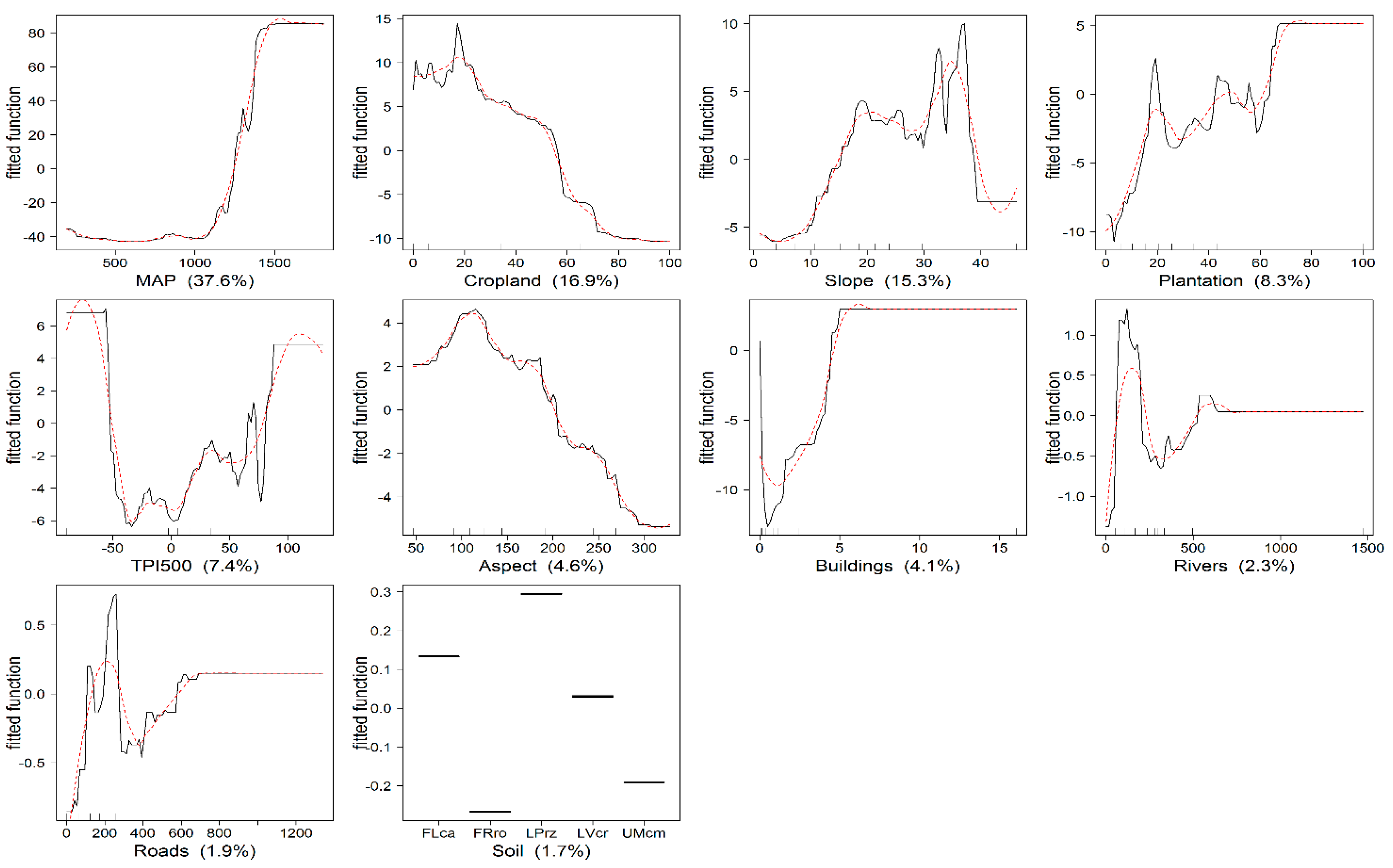
Figure 5.
The strongest interactions between the explanatory variables in the fitted boosted regression trees (BRT) model: (a) cropland vs. mean annual precipitation (MAP), (b) slope vs. MAP, (c) aspect vs. slope and (d) cropland vs. slope. Note that the plots have different scaling for the Y-axis.
Figure 5.
The strongest interactions between the explanatory variables in the fitted boosted regression trees (BRT) model: (a) cropland vs. mean annual precipitation (MAP), (b) slope vs. MAP, (c) aspect vs. slope and (d) cropland vs. slope. Note that the plots have different scaling for the Y-axis.


Table 1.
Descriptive statistics for the field plots (n = 215).
| Attribute | Range | Median | Mean | SD |
|---|---|---|---|---|
| Density (stems/ha) | 10–1214 | 160 | 309 | 301 |
| Basal area (m2) | 0.1–94.3 | 9.2 | 19.9 | 21.6 |
| Mean DBH (cm) | 10.4–46.1 | 22.4 | 23.5 | 7.2 |
| Lorey’s mean height (m) | 3.0–39.3 | 12.6 | 13.8 | 7.0 |
| AGB (Mg/ha) | 0.1–671.3 | 37.9 | 123.0 | 153.0 |
Table 2.
Scanner properties and flight parameters of the ALS data.
| Parameter | Value |
|---|---|
| Dates of acquisition | 2014 (26 January, 6 February and 8 February) and 2015 (5, 6, 11 and 13 February) |
| Sensor | Leica ALS60 |
| Mean range (m) | 1460 |
| Pulse rate (kHz) | 58 |
| Scan rate (Hz) | 66 |
| Scan angle (°) | ±16 |
| Mean Pulse density (pulses m−2) | 3.1 |
| Range of Pulse density (pulses m−2) | 1.0–4.9 |
| Mean return density (returns m−2) | 3.4 |
| Beam divergence at 1/e2 (mrad) | 0.22 |
| Mean footprint diameter (cm) | 32 |
Table 3.
Summary of airborne laser scanning (ALS) metrics.
| Metric | Description |
|---|---|
| H.p01, H.p05, H.p10, H.p20, H.p25, H.p30, H.p40, H.p50, H.p60, H.p70, H.p75, H.p80, H.p90, H.p95, H.p99 | 1st, 5th, 10th … and 99th percentile of return heights >3 m |
| H.max | Maximum of return heights >3 m |
| H.mean | Mean of return heights >3 m |
| H.cv | Coefficient of variation of return heights >3 m |
| H.stdev | Standard deviation of return heights >3 m |
| H.skewness | Skewness of return heights >3 m |
| H.kurtosis | Kurtosis of return heights >3 m |
| CC.first | First returns >3 m/total first returns × 100 |
| CC.all | All returns >3 m/total all returns × 100 |
| CC.all.first | All returns >3 m/total first returns × 100 |
| CC.first.mean | First returns above mean/total first returns × 100 |
| CC.all.mean | All returns above mean/total all returns × 100 |
| CC.all.mean.first | All returns above mean/total first returns × 100 |
Table 4.
Explanatory variables for aboveground biomass modelling.
| Variable | Description | Resolution (m) |
|---|---|---|
| Topography, hydrology and soil | ||
| Elevation | Elevation (m a.s.l.) based on DEM | 5 |
| Slope | Slope (°) based on DEM | 5 |
| Aspect | Aspect (°) based on DEM | 5 |
| TPI50–TPI500 | Topographic position index (TPI) with 50 m, 100 m, 150 m, 200 m, 300 m and 500 m radii based on DEM | 5 |
| TWI | Topographic wetness index based on DEM | 5 |
| Rivers | Length of rivers (m); river network extracted from DEM | 10 |
| Soil | Soil type vector layer from the Soil Atlas of Africa | - |
| Climate | ||
| MAT | Mean annual temperature (°C) | 20 |
| MAP | Mean annual precipitation (mm) | 20 |
| Land use | ||
| Cropland | Cropland cover (%) based on the LULC map | 20 |
| Plantation | Plantation forest cover (%) based on the LULC map | 20 |
| Building | Cover (%) of buildings extracted from ALS point cloud | 2 |
| Road | Length (m) of road digitized from the high-resolution imagery | - |
Table 5.
Summary of the final model for AGB mapping. H.p25 = 25th percentile point of all laser return heights above 3 m; CC.all.first = all returns above 3 m/total first returns × 100; *** p < 0.001.
Table 5.
Summary of the final model for AGB mapping. H.p25 = 25th percentile point of all laser return heights above 3 m; CC.all.first = all returns above 3 m/total first returns × 100; *** p < 0.001.
| Dependent Variable | Explanatory Variables | Estimate | SE of Estimate |
|---|---|---|---|
| Intercept | 0.423 *** | 0.268 | |
| H.p25 | 0.372 *** | 0.033 | |
| CC.all.first | 0.086 *** | 0.005 |
© 2017 by the authors. Licensee MDPI, Basel, Switzerland. This article is an open access article distributed under the terms and conditions of the Creative Commons Attribution (CC BY) license (http://creativecommons.org/licenses/by/4.0/).
Share and Cite
MDPI and ACS Style
Adhikari, H.; Heiskanen, J.; Siljander, M.; Maeda, E.; Heikinheimo, V.; K. E. Pellikka, P. Determinants of Aboveground Biomass across an Afromontane Landscape Mosaic in Kenya. Remote Sens. 2017, 9, 827. https://doi.org/10.3390/rs9080827
AMA Style
Adhikari H, Heiskanen J, Siljander M, Maeda E, Heikinheimo V, K. E. Pellikka P. Determinants of Aboveground Biomass across an Afromontane Landscape Mosaic in Kenya. Remote Sensing. 2017; 9(8):827. https://doi.org/10.3390/rs9080827
Chicago/Turabian StyleAdhikari, Hari, Janne Heiskanen, Mika Siljander, Eduardo Maeda, Vuokko Heikinheimo, and Petri K. E. Pellikka. 2017. "Determinants of Aboveground Biomass across an Afromontane Landscape Mosaic in Kenya" Remote Sensing 9, no. 8: 827. https://doi.org/10.3390/rs9080827
Note that from the first issue of 2016, this journal uses article numbers instead of page numbers. See further details here.