An Improved Vegetation Adjusted Nighttime Light Urban Index and Its Application in Quantifying Spatiotemporal Dynamics of Carbon Emissions in China


1
School of Geographical Sciences, East China Normal University, Dongchuan Road 500, Shanghai 200241, China
2
Shanghai Key Laboratory for Urban Ecological Processes and Eco-Restoration, School of Ecological and Environmental Sciences, East China Normal University, Dongchuan Road 500, Shanghai 200241, China
*
Author to whom correspondence should be addressed.
Remote Sens. 2017, 9(8), 829; https://doi.org/10.3390/rs9080829
Submission received: 30 May 2017
/
Revised: 27 July 2017
/
Accepted: 9 August 2017
/
Published: 11 August 2017
(This article belongs to the Special Issue Recent Advances in Remote Sensing with Nighttime Lights)
Abstract
:Nighttime Light (NTL) has been widely used as a proxy of many socio-environmental issues. However, the limited range of sensor radiance of NTL prevents its further application and estimation accuracy. To improve the performance, we developed an improved Vegetation Adjusted Nighttime light Urban Index (VANUI) through fusing multi-year NTL with population density, the Normalized Difference Vegetation Index and water body data and applied it to fine-scaled carbon emission analysis in China. The results proved that our proposed index could reflect more spatial variation of human activities. It is also prominent in reducing the carbon modeling error at the inter-city level and distinguishing the emission heterogeneity at the intra-city level. Between 1995 and 2013, CO2 emissions increased significantly in China, but were distributed unevenly in space with high density emissions mainly located in metropolitan areas and provincial capitals. In addition to Beijing-Tianjin-Hebei, the Yangzi River Delta and the Pearl River Delta, the Shandong Peninsula has become a new emission hotspot that needs special attention in carbon mitigation. The improved VANUI and its application to the carbon emission issue not only broadened our understanding of the spatiotemporal dynamics of fine-scaled CO2 emission, but also provided implications for low-carbon and sustainable development plans.
1. Introduction
Nighttime Light (NTL), derived from the Defense Meteorological Satellite Program’s Operational Linescan System (DMSP/OLS), has become one of the most widely-used data for interpreting some socio-environmental issues that are difficult to understand at a relatively high spatial resolution, such as economic output [1,2], urbanization [3,4,5], poverty [6,7,8], energy consumption and greenhouse gas emissions [9,10,11]. Methods and indicators based on NTL are usually labor saving and unbiased compared to those grounded on statistical data. It is especially crucial for increasing our understanding of the spatiotemporal dynamics of the aforementioned issues and thus helping us to make proper and timely decisions toward sustainability [12].
On the one hand, despite the endeavors made by previous studies to improve NTL data, some defects still exist, which may constrain the further application and estimation accuracy. First, because of the limited radiance range of the OLS sensor, pixels with weak radiance (<10−10 watts/cm2/sr/mm), which often exist in developing countries or hamlets, cannot be detected and are often given the value of zero [13]. Consequently, the estimations in these unlit pixels might be missing [14,15]. Second, the saturation problem in the downtown area and the blooming effect in the suburbs of DMSP/OLS NTL may cause the estimation to deviate from the reality [16,17,18]. To deal with these problems, various methods and indices have been developed generally through fusing NTL with other data sources. For example, some used population density to increase the variation of NTL in urban cores and supplemented information of human activities for unlit pixels [14,19]. Assuming that vegetation cover and human activities are inversely correlated, some combined Normalized Difference Vegetation Index (NDVI) with NTL to reduce the saturation effect of NTL [20,21,22]. Specifically, the Vegetation Adjusted NTL Urban Index (VANUI), which is defined as (1 − NDVI) × NTL, was a simple and effective index for reducing the saturation effect in urban areas [23]. It has been employed as a better proxy than the original NTL in studying urban impervious surfaces [24]. However, some research also argued that VANUI might result in estimation error in some regions with a diverse natural environment and vegetation cover, such as western cities in China [24,25]. Additionally, the investigations using long-term time series VANUI are still not fully addressed. The development of improved methods and indicators that have high accuracy and can effectively address the spatiotemporal dynamics of socio-environmental issues are increasingly needed.
On the other hand, CO2 emissions and their mitigation have become one of the most crucial challenges for sustainable development faced by all of the countries in the world. Fossil fuel-related CO2 emissions contributed to more than 70% of the total greenhouse gas emissions, which cause profound impacts on physical, biological and socioeconomic systems, such as global warming, sea level rise, biodiversity loss, agricultural productivity decline and urban heat islands [26,27,28]. However, the lack of authentic and reliable statistical data on energy consumption prevents a better investigation of the spatiotemporal dynamics of CO2 emissions at a finer scale, which is crucial for local governments to adapt to and mitigate climate change efficiently [29,30,31]. Taking China, the largest carbon emitter since 2006 [32], as an example, it has set a 60~65% reduction target of CO2 emissions intensity by 2030 below its 2005 level [33]. In order to decompose the mitigation target to local administrative units (for example, cities), it is important to understand the spatial distribution of CO2 emissions and its change at various scales [34]. Many studies have explored the spatiotemporal dynamics at the country or province level based on statistics [35,36]. However, the biggest challenge faced by policy makers and researchers is the data availability at the prefectural city or even finer levels since the detailed information on the amount and structures of energy consumption at those levels is not open to the public or fragmented. Luckily, NTL provides a possible solution to fill this gap. Previous studies have proven that it was feasible to estimate CO2 emissions at the 1-km spatial level using NTL [37]. Yet, few studies focused on the potential estimation errors caused by NTL at a fine scale. For example, CO2 emissions in unlit pixels might be missing; emissions in urban core areas might be underestimated, caused by the saturation problem; while emissions in suburban areas might be overestimated because of the blooming effect. Again, it is quite necessary to develop improved methods and indicators based on NTL to expand our knowledge of carbon emissions.
To this end, we developed an improved VANUI, which combines NTL with time series NDVI, population density and water body data to calibrate the saturation and blooming problems and to reduce the estimation error in the urban core and rural areas and, then, applied it to the carbon emission issue in China, so that the performance of the proposed index can be tested and our understandings of a fine-scaled CO2 emission dynamics can also be increased. This paper is organized as follows: Section 2 describes the study area, as well as the data we used. Section 3 introduces the methods for developing an improved VANUI, downscaling statistically accounted CO2 emissions to fine spatial scales, verifying the model accuracy and analyzing the spatiotemporal dynamics of CO2 emissions. Section 4 analyzes the results. Section 5 discusses the performance of the proposed new index and provides potential uses for further studies, followed by conclusions in Section 6.
2. Study Area and Data Description
2.1. Study Area
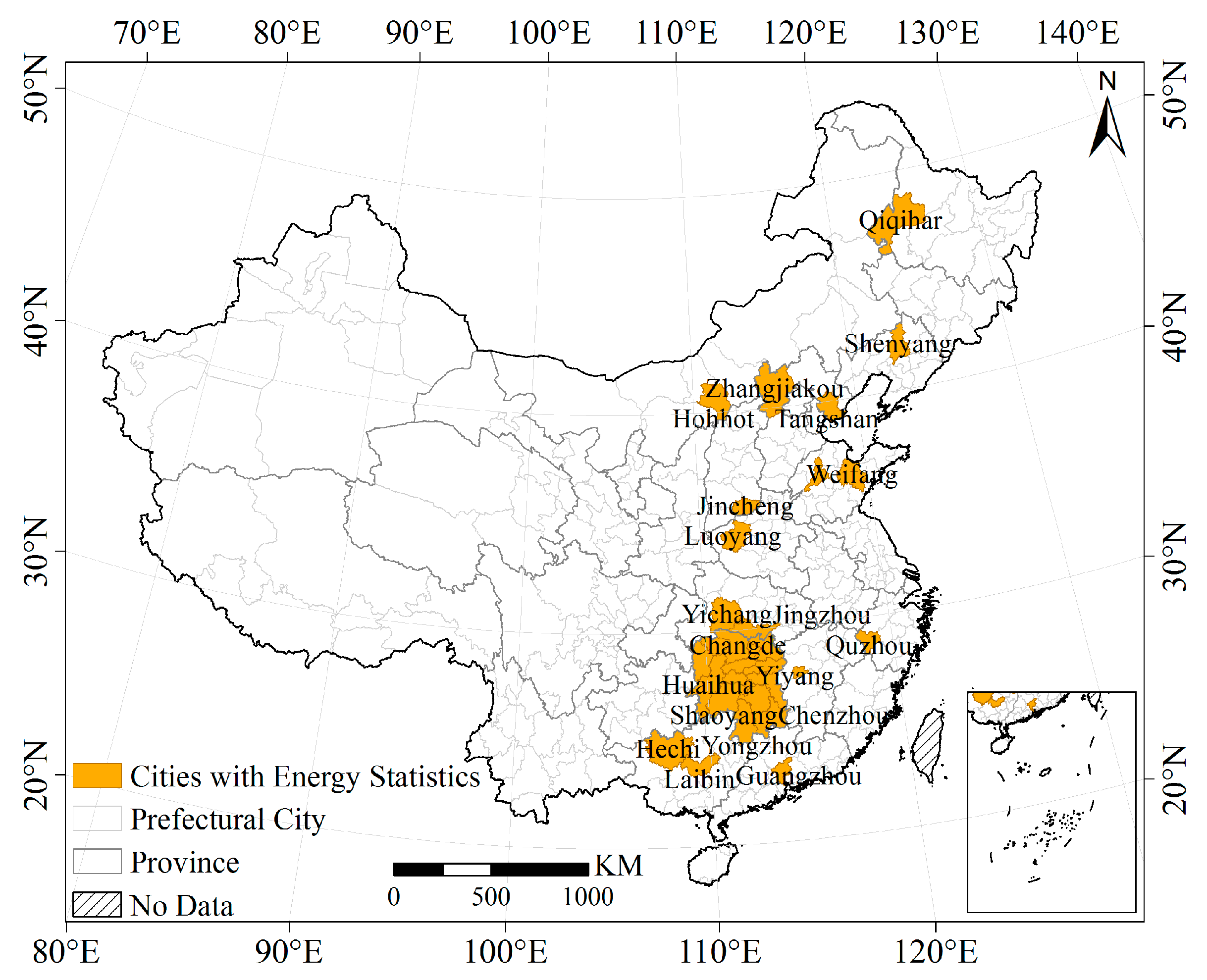
The jurisdiction units in China are organized under a country-province/municipality-prefectural city-county hierarchy. As shown in Figure 1, detailed energy statistical data for accounting for CO2 emissions are only available for the whole country, 30 provinces/municipalities (Tibet lacks data) and 30 prefectural cities from 1995. Table 1 provides a summary of the socioeconomic conditions for those 30 cities having detailed energy statistics. However, the same energy inventories for most cities and counties are not available, thus they cannot facilitate a long-term CO2 emissions study at those scales.
2.2. Data Description
Table 2 gives a summary of data used for analysis, which generally include energy statistics and seven kinds of geospatial data.
In order to calculate CO2 emissions from energy consumption in China at provincial and some specific prefectural city level, the amounts of 11 types of energy were collected based on provincial and local energy balance tables from China’s Energy Statistical Yearbook [38] and relevant City Statistical Yearbooks of 30 prefecture-level cities as shown in Figure 1. In addition, heat and electricity were also included in the CO2 accounting scopes, which were obtained from the same sources.
The Version 4 DMSP/OLS NTL series record lights on the Earth’s surface generated from persistent light in cities, towns and other human settlements and other light from gas flares, fires and illuminated marine vessels. The annual average brightness was presented as six-bit digital numbers (DN) from 0–63 after compositing the highest quality data avoiding interference from sunlit, glare, moonlit, clouds and features from the aurora in a whole year. They spanned −180–180 degrees in longitude and −65–75 degrees in latitude, with 30 arc second grids.
The maximum Moderate-resolution Imaging Spectroradiometer (MODIS) NDVI time series were calculated based on the MOD09GA images from EOS/MODIS using Maximum Value Composites (MVC), after splicing, cutting, projection conversion and unit conversion. The space resolution of the dataset was 500 m × 500 m, and the temporal resolution was a month. Images from January 2000–December 2013 were used in this study. Besides, the Global Inventory Monitoring and Modeling System (GIMMS) NDVI dataset was generated based on the NOAA/AVHRR land dataset after radiometric calibration, geometric correction and cloud elimination, with a spatial resolution of 8 km × 8 km and a temporal resolution of 15 days. Images from January 1995–December 1999 were used as a supplement to fill the data gap between 1995 and 1999. In addition, in order to obtain consistent and comparable NDVI, images from January 2000–December 2006 were employed as samples to capture the relationship between NDVIs from two sensors. In order to match the temporal resolution of MODIS NDVI, monthly GIMMS NDVI data were compiled by the MVC method.
Gridded population density data in China of 1995, 2000, 2005 and 2010 were obtained from the Resources and Environmental Sciences Data Center, Chinese Academy of Sciences (RESDC). The multivariate statistical population spatial model was used for these data based on demographic statistics at a county level and land use/cover data at a spatial resolution of 1 km × 1 km. Besides, urban population density, DEM and the total population were used to ensure that the model results were accurate and reasonable [39].
Moreover, the water body distribution map was used as a mask to eliminate the potential interference caused by low NDVI in water bodies in this paper. All images were projected into the Lambert Azimuthal Equal Area Projection with reference to World Geodetic System 1984 (WGS 84), resampled to a spatial resolution of 1 km × 1 km by the nearest neighbor resampling algorithm and extracted by the multilevel administrative boundaries of China. Besides, four Landsat 8 Operation Land Imager (OLI) images in 2013 covering Beijing, Shanghai, Guangzhou and Urumqi were selected as references to assess the estimation accuracy.
3. Methods
Figure 2 presents the methodological framework, which includes three major steps. Firstly, an improved VANUI was developed based on the integration of NTL, NDVI, population density and water body data. Secondly, statistically accounted CO2 emissions at the provincial level were downscaled to a 1-km spatial resolution based on the improved VANUI. Additionally, the accuracy of the prosed new index was validated. Thirdly, the spatiotemporal dynamics of CO2 emissions at the pixel and prefecture-city level were explored.
3.1. An Improved Time-Series VANUI
Because the original time series NTL were obtained from different satellite sensors (F12, F14, F15, F16 and F18), they lack continuity and cannot be used directly for long-term analysis. A systematic calibration approach, which was developed by Liu et al. [40] and included inter-calibration, intra-annual composition and inter-annual series correction processes, was employed in this study to calibrate the original NTL data in China. Besides, the following model proposed by Meng et al. [14] was used to adjust NTL in the lit and unlit areas:
where is the NTL adjusted by population density; NTLcali is the original night time images after a series of calibration processes proposed by Liu et al. [40]; POP is the population density; 0.34 is the weight for the unlit areas based on the detected electricity access in lit and unlit areas of NTL [41]. Specifically, the gridded population density of 1995, 2000, 2005 and 2010 was used to calibrate NTL for the years of 1995~1998, 1999~2003, 2004~2008 and 2009~2013, respectively.
We used two datasets of NDVI to satisfy the research period in this paper because MODIS NDVI images are unavailable before 2000. However, the monthly NDVI data from different sensor systems could not be calculated directly because they lack consistency and comparability. Early studies have proven that NDVI from one instrument can be inter-calibrated against another by linear regression models [42]. To ensure the consistency of NDVI data from two sensors, we built a linear regression model based on monthly 1-km GIMMS NDVI and MODIS NDVI in China from 2000–2006 (Figure 3) and finally obtained the following model.
where NDVIMODIS and represent monthly 1-km MODIS NDVI and GIMMS NDVI datasets, respectively.
The annual mean NDVI time series from 1995–2013 were then calculated. However, unlike MVC, which could reduce the impacts of cloud and shadow of NDVI, the mean NDVI can reduce seasonal sensitivity and fluctuation and, thus, is more stable than the max NDVI [23]. Negative NDVI values were removed because they indicate deserts, glaciers and other areas with few human activities [43,44].
The improved VANUI in China from 1995–2013 was then computed using the following model [23]:
where NDVI is the annual mean NDVI; is the normalized value of the NTL adjusted by population density ranging from 0–1, which can be calculated by:
where and are the maximum and minimum values of from 1995–2013.
Similar to Liu’s approach to improve the annual consistence of DMSP/OLS NTL during a long time period [40], the annual improved VANUI should be calibrated by Equation (5) on the basis of the following assumptions: (1) the pixel level adjusted VANUI grew continuously in China during the last 19 years, and the value in a later year should be equal to or greater than that in the previous year; (2) the adjusted VANUI in 2013 was the largest and closest to reality in the time series. We chose the adjusted VANUI in 2013 instead of VANUI in 1995 as the reference data because VANUI in 2013 was calculated based on MODIS NDVI, which have higher quality than those in 1995.
where t = 1, 2, …, 18; T is the latest year of the study period (that is 2013 in this research); is the VANUI that needs to be calibrated in the year of T − t (i.e., from 2012–1995); is the improved VANUI from 2012–1995 calculated before; is the improved VANUI in the next year of .
3.2. Estimating CO2 Emissions Using Improved VANUI
First, CO2 emissions from 30 provinces are accounted so as to provide training samples for further downscaling analysis. The guideline proposed by the Intergovernmental Panel on Climate Change (IPCC) was adopted as a standard method for carbon accounting [45]:
where represents the statistical CO2 emissions of the sample province; the subscript k denotes the energy type; FC is total fuel consumption; EF is the effective CO2 emission factor; LC is the low calorific value of each fuel; CC represents carbon content; CR is the carbon oxidation ratio; 44/12 is the molecular weight ratio of carbon dioxide to carbon. The EF of electricity was the mean annual EF of seven power sub-grids in China from 2007–2013, provided by National Development and Reform Commission (NDRC) [46]. Others were compiled from the Provincial Greenhouse Gas List published by NDRC [47]. Table 3 provides the parameters for emissions accounting.
Second, a linear regression model, as shown in Equation (7), was employed to capture the relationship between statistically accounted CO2 emissions from sample provinces and improved VANUI:
where denotes the total improved VANUI value in corresponding provinces; and are the intercept and coefficient, which need to be estimated.
In this study, 19 regression models from 1995–2013 were built to reduce the temporal bias in estimating CO2 emissions. As shown in Table 4, all parameters were significant at the 5% or 1% level based on the t-test, with reasonable values of the coefficient of determination R2 (R2 > 0.75), suggesting that the improved VANUI is an appropriate proxy of CO2 emissions. One possible reason for the increasing R2 after 2000 might be that the quality of VANUI calculated by MODIS NDVI after 2000 is higher than those calculated by GIMMS NDVI because of the higher spatial resolution of the original MODIS NDVI (500 m).
Assuming the relationship between CO2 emissions and improved VANUI at the pixel level was consistent with that at the sample province level, the following model was used to downscale provincial CO2 emissions to the pixel level:
where represents the CO2 emissions estimated by the improved VANUI at the pixel level; is the total lit pixels in the province; is the value of improved VANUI in the pixel; others are the same as for Equation (7).
Furthermore, to limit the estimation residuals within a province, the estimated pixel-level CO2 emissions by Equation (8) were corrected by the following equation:
where is the modeled pixel-level CO2 emissions after correction. is the sum of pixel-level estimated CO2 emissions () within each provincial boundary. It was noted that since Tibet Province lacks energy statistical data, pixel-level CO2 emissions within Tibet could not be corrected through Equation (9), but directly use the estimations by Equation (8).
3.3. Assessing the Accuracy of Improved VANUI in Modeling CO2 Emissions
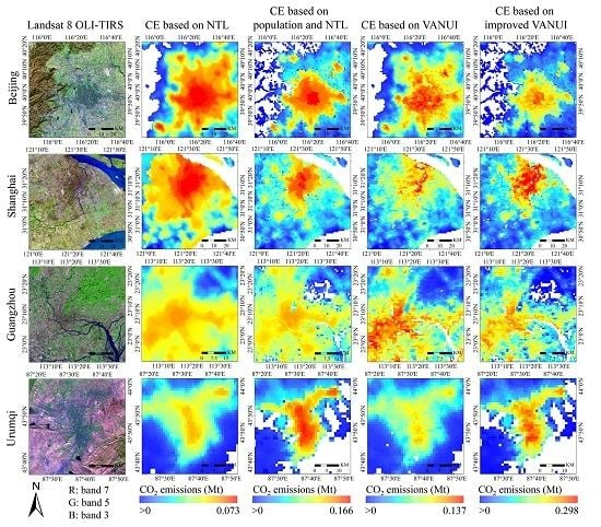
Due to the lack of high-resolution CO2 emissions for a reference, we used two assessments to evaluate the performance of improved VANUI in modeling CO2 emissions. First, the root mean square error (RMSE) and mean relative error (MRE) were used to describe the difference between the modeled CO2 emissions and statistically accounted emissions from 30 prefecture cities that have detailed energy statistics (the accounting method was the same as that at the provincial level). Second, since CO2 emissions from impervious areas are usually higher than those from dense vegetation covered areas [36], Landsat 8 OLI-TIRS images of four selected cities in China, including Beijing and Shanghai (typical mega cities that usually have the NTL saturation phenomenon), Guangzhou and Urumqi (typical cities with distinct natural environment and vegetation covers) were used as references to assess whether the improved VANUI could reflect this emission difference within the same city.
3.4. Analyzing Spatiotemporal Patterns of Prefecture-City Level CO2 Emissions
Indicators including Global Moran’s I, and Anselin Local Moran’s I (Local indicators of spatial association, LISA) were used to explore the spatiotemporal patterns of prefecture-city level CO2 emissions. Specifically, Global Moran’s I measures the spatial autocorrelation of prefectural CO2 emissions nationwide [48].
where n is the total number of prefectural cities; i and j are two different cities; is the spatial weights matrix, which was decided by the criteria of the first-order queen contiguity in this study; and are the modeled CO2 emissions for city i and j, respectively; is the average emissions of the whole study area. With the value ranging from −1–1, Global Moran’s I evaluates whether the spatial distribution of CO2 emissions is random (=0), clustered (>0) or dispersed (<0).
LISA shows the spatial dependence and heterogeneity among prefectural cities [33].
where Zi is the deviation of modeled emissions for city i from the average and is the spatial lag for city i, which reflects the weighted average of CO2 emissions from the neighboring city j, and can be calculated by .
Based on whether both Zi and are higher than 0 or not, cities could be classified into four cluster types. They are high-high clusters (Zi > 0 and > 0), high-low clusters (Zi > 0 and < 0), low-high clusters (Zi < 0 and > 0) and low-low clusters (Zi < 0 and < 0). The LISA results can be used to provide visual information of local instability in spatial autocorrelation [49].
4. Results
4.1. Performance Test of the Improved VANUI
To evaluate the capability of the improved VANUI in tackling the saturation and blooming problems, we compared the normalized value of original NTL, population-adjusted NTL (calculated by Equations (1) and (4)), original VANUI and improved VANUI in a line transect in the Beijing-Tianjin-Tangshan metropolitan area. It was found that the values of the original NTL were obviously saturated in the urban center of Beijing (Figure 4b). Although population-adjusted NTL could help to reduce the saturation, the improvements in some urbanized areas were still not as much as expected. For instance, the pixel range of population-adjusted NTL in Figure 4c was still close to one. Notably, both the original and improved VANUI captured more spatial details in urban center areas with their values much lower than other two indices. In suburban areas, the capability of original NTL and original VANUI in describing the human activity variation was weak. For example, the values in the 0–20 pixel range in Figure 4b,d were close to zero and had little change. Large fluctuations in population-adjusted NTL and improved VANUI values could be detected (for example, the pixel range of 12–13 in Figure 4c,e), which suggested that they could supplement more information of the human activity differences. In sum, the improved VANUI can reflect human activities more accurately, which is crucial for interpreting socio-environmental issues.
4.2. Accuracy Assessment of Improved VANUI in Modeling CO2 Emissions
Using the same methods described in Section 3.2, CO2 emissions were additionally modeled based on the original NTL, the population-adjusted NTL and the original VANUI and compared to that based on the improved VANUI so that the accuracy of improved VANUI in modeling CO2 emissions can be assessed. The comparisons were conducted at the following two levels.
First, at the inter-city level, as shown in Figure 5, statistically accounted CO2 emissions from 30 prefecture cities that have detailed energy statistics between 1995 and 2013 (in total, 170 samples) were accounted as references by the same method described in Section 3.2. It was found that the R2 in the correlation between statistical CO2 emissions and modeled emissions derived from the improved VANUI was the same as that in the original VANUI’s case (R2 = 0.64), but was higher than that in the original NTL’s case (R2 = 0.59) and the population-adjusted NTL’s case (R2 = 0.52). More importantly, the modeled CO2 emissions using the improved VANUI owned the lowest RMSE and MAE compared to the others, which suggested that improved VANUI was more accurate in modeling CO2 emissions at the inter-city level.
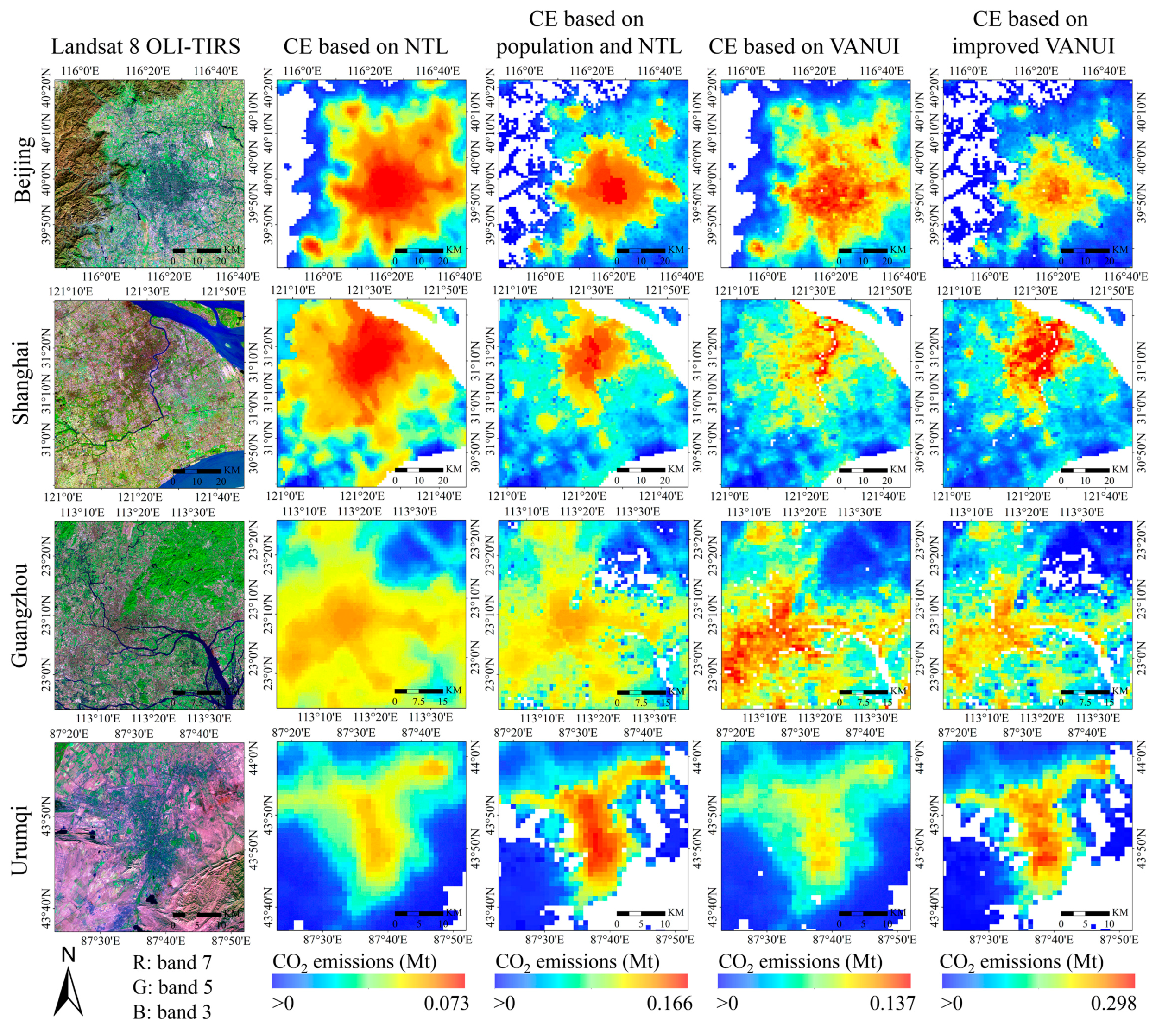
Second, at the intra-city level, Figure 6 shows the modeled CO2 emissions (CE) in Beijing, Shanghai, Guangzhou and Urumqi based on four indices. Landsat 8 OLI images in 2013 were used for visual references. The modeled results varied significantly in the four cases. Obviously, the variation of emission density using improved VANUI was the largest with the maximum value around 0.30 million tons/km2, which was 4.2-, 1.8- and 2.2-times larger than that in the original NTL, population-adjusted NTL and original VANUI, respectively. This result implied that improved VANUI could strengthen the heterogeneity at the intra-city level. In addition, it was found that CO2 emissions modeled by improved VANUI could reduce the saturation effect and estimation deviation significantly. Due to the blooming problem, emissions based on the original NTL in urban parks and suburbs were usually overestimated, while being underestimated in sub-centers. In the population-adjusted NTL’s case, emissions in suburban regions were much lower than those in urban cores, but the saturation phenomenon at the center area of mega cities was still serious. As for the original VANUI-based emissions, though VANUI can capture more details in urban cores, its performance in suburban areas with less vegetation cover (for example, suburban Urumqi) was not satisfactory. Moreover, emissions in urbanized areas with low NDVI, but high NTL might be overestimated (for example, river zones in Shanghai and Guangzhou). By contrast, the relatively low emissions in urban parks and high emissions in urban cores and sub-centers have been successfully distinguished through improved VANUI.
4.3. Spatiotemporal Dynamics CO2 Emissions in China
Figure 7 shows the spatial pattern of the modeled pixel-level CO2 emissions in China from 1995–2013. It is found that CO2 emissions mainly concentrated in Eastern and Southeastern regions. Visually, the CO2 emission density in metropolitan areas and provincial capital cities was much higher than that in small cities and rural areas. The highly urbanized areas including Beijing-Tianjin-Hebei (BTH), the Yangtze River Delta (YRD) and the Pearl River Delta (PRD) witnessed a sharp increase in emissions, where the emission density has more than doubled from 0.14–0.30 million tons/km2 between 1995 and 2013.
By aggregating the pixel level CO2 emissions to prefecture cities and analyzing the spatiotemporal characteristics, it was noted that the results of Global Moran’s I were significantly positive during the study period, which indicated the existence of spatial agglomeration of CO2 emissions in Chinese cities (Figure 8). In other words, cities with similar emissions tended to cluster in space. However, the degree of agglomeration underwent a decrease from 0.31 in 1995 to 0.20 in 1999, then an increase to 0.36 in 2007 and, finally, became relatively stable around 0.35 from 2008–2013. The differences in regional development strategy and socioeconomic conditions might be one of the main reasons for the changing level of agglomeration. For example, the quick catching up of the economy in inland regions of China due to a series of favorable development strategies and plans, such as the “Grand Western Development Program” since 2000 and the “Rise of Central China Plan” since 2004, may explain the growth of the agglomeration degree in the beginning of the 2000s. Moreover, great efforts were made by the Chinese government to encourage energy conservation and emissions reduction at the country level, such as the implementation of the “Medium and Long-Term Energy Conservation Plan” launched in 2004, the “11th Five Year Plan (2006–2010)” and the “12th Five Year Plan (2011–2015)”, which could be the important reasons why agglomeration of CO2 emissions kept stable after 2007 [50,51].
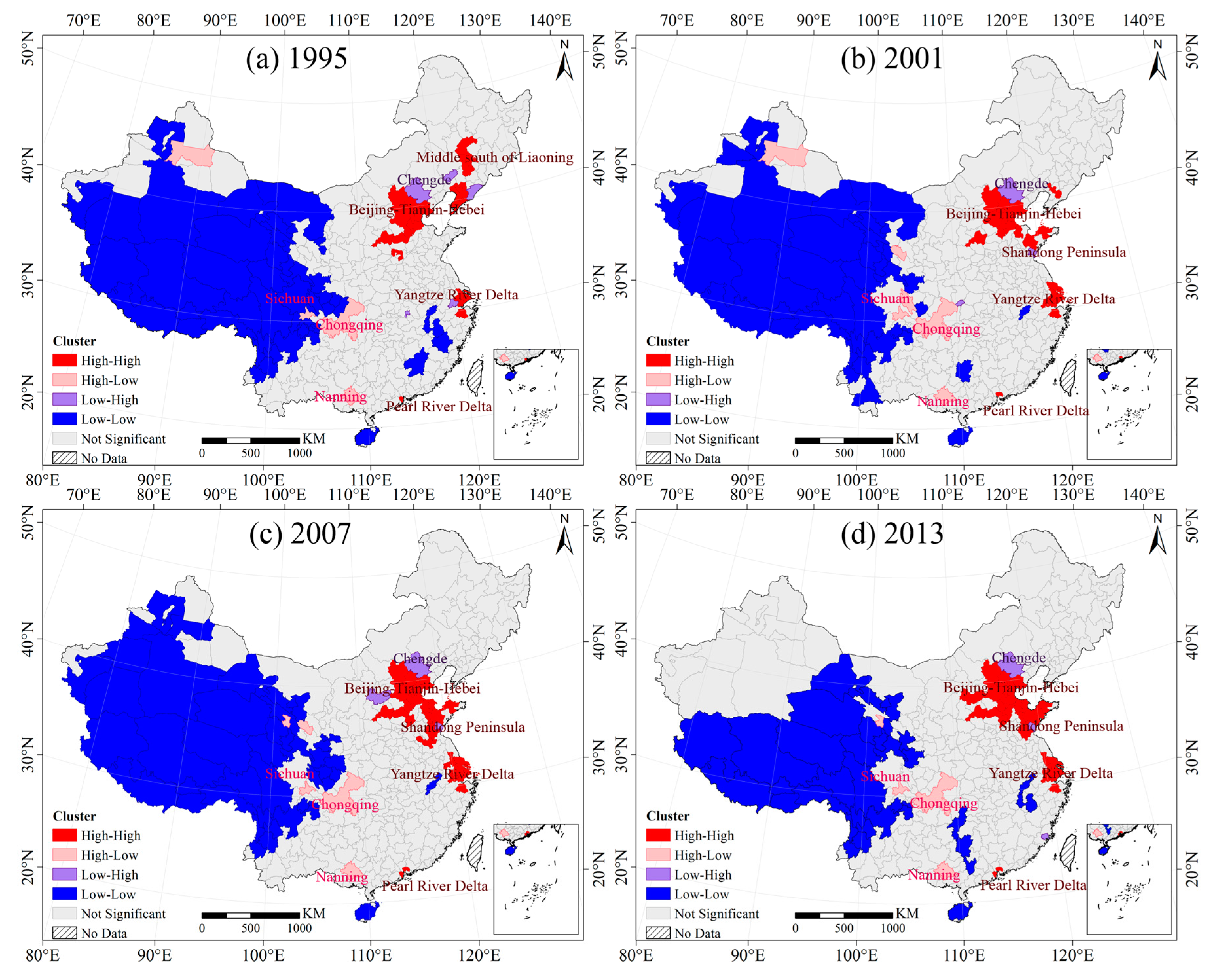
Figure 9 shows the results of LISA for 343 prefecture cities. Based on four types of clusters, the hot spots of carbon emissions and spatially-heterogeneous areas can be identified. Most of the clusters are spatially coherent. BTH, YRD and PRD belonged to the high-high clusters, suggesting that these areas were hot emission spots that need special attention in carbon mitigation. Notably, because of the rapid development of the Bohai Economic Rim in recent years, Shandong Peninsula has replaced the middle south Liaoning, a traditional heavy industrial region in Northeastern China, and became a new cluster with large emissions. The low-low clusters mainly located in the western region and have become less extensive. Most of these clusters were located in Tibet, Qinghai and Gansu provinces, which have less population and carbon-intensive industries. Chongqing and Nanning were labeled as high-low clusters with more CO2 emissions than their neighboring cities. On the contrary, Chengde, a city next to Beijing, emitted much less CO2 than its neighbors did.
5. Discussion
5.1. Comparison with Previous Studies
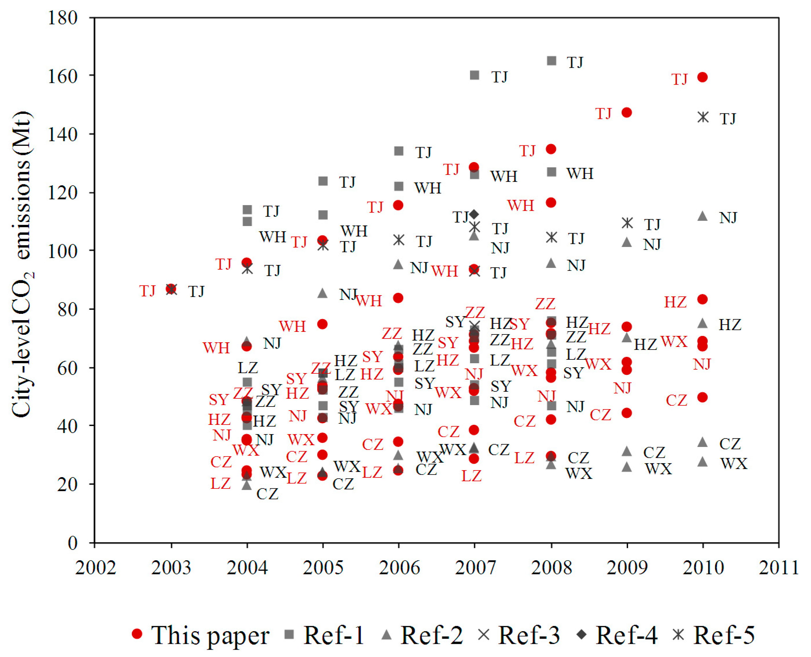
By comparing our modeled CO2 emissions in some selected cities and years with those from previous studies, most of which are based on statistical data and methods, the robustness and reliability of our proposed methods can be validated. As shown in Figure 10, there were big differences in each study even for the same city based on the same accounting framework. Taking Tianjin as an example, our estimate results were smaller than those from Ref-1, but larger than those of Ref-5. The different accounting scopes and methods might be the main reason for these differences, as Ref-1 accounted the carbon emissions from industrial processes while we did not, and we considered the emissions from electricity and heating, while Ref-5 ignored them. Regardless, the changing trend and scale of all of the results are similar to each other, which suggested the validity of our estimation based on the improved VANUI.
5.2. Limitations and Potential Uses
Though the proposed methods are proven to be effective and accurate in analyzing the carbon emission issue, there remains several limitations that could be further improved in the future study. First, we did not take into account the uncertainties from emission factors and energy consumption data when accounting CO2 emissions based on statistics, which could vary from ±5–±10% [57,58]. It was also pointed out that the poor quality of energy statistics would cause significant discrepancy between national and provincial emissions in China [59]. All of these will influence the model accuracy since the statistically accounted CO2 emissions are among the fundamental bases of our methods.
Second, although the estimation error of improved VANUI was the smallest, there still exist big gaps between modeled and statistically accounted emissions for some cities (as shown in Figure 5). More efforts in improving the data quality and integrating more variables in model algorithms should be made. Specifically, since CO2 emissions are not only driven by demographic factors, economic level and structure, local biophysical conditions such as temperature, elevation and urban form are also reported as important determinants [60,61,62]. In the future, with the emergence and development of big data science, it might be possible to obtain detailed spatial data of the aforementioned variables through the Internet, social media, commercial data companies, and so on, for enhancing the performance of NTL.
Owing to the global coverage of NTL and NDVI and the increasing availability of spatial data for population and land use and cover in the world (for example, Landscan’s population data with 1-km resolution [63] and Global Land Project’s land use and cover maps with 30-m resolution [64], our proposed methods could also be applied to other countries and regions and to other socio-environmental issues, such as steel stocks’ distribution in human society and residential energy consumption.
6. Conclusions
By improving the original VANUI via the integration of NTL with NDVI, population density and water body distribution, this paper proposed a new index to enhance the performance of DMSP/OLS NTL, so that it can be better applied in analyzing socio-environmental issues. China was selected as a case to validate the accuracy of improved VANUI in modeling fine-scaled CO2 emissions and to increase our understandings of its spatiotemporal dynamics from 1995–2013.
The findings can be concluded as follows. First, the improved VANUI can supplement more information of human activities in areas with weak radiance, which cannot be detected by the original NTL. Second, it can reduce estimation errors in downtown areas and suburbs caused by the saturation and blooming problems of NTL. Third, the improved VANUI shows great potential to be further applied as a proxy of many socio-environmental and socioeconomic issues, especially in regions that are lack of sufficient and reliable statistical data. Fourth, with the aid of improved VANUI, it is found that carbon emission density in metropolitan areas and provincial capitals was much higher than in small cities and rural areas. Global Moran’s I confirmed the existence of the spatially-agglomerated distribution of CO2 emissions in China. In addition to the BTH, YRD and PRD regions, Shandong Peninsula replaced the middle south Liaoning and became a new emission hotspot. These findings may increase our understanding of the spatiotemporal dynamics of CO2 emissions and provide decision-making support to design sustainable development plans and low-carbon policies.
Acknowledgments
The work was supported by the National Key R&D Program of China (Grant Number 2017YFC0505703); the National Natural Science Foundation of China (Grant Number 41401638, 41471076); the Ministry of Education in China Project of Humanities and Social Sciences (Grant Number 14YJAZH028); the Shanghai Philosophy of Social Sciences Planning Project (Grant Number 2014BCK001).
Author Contributions
Ji Han and Xing Meng designed the research. Xing Meng performed the calculations, analyzed the results and wrote the manuscript. Ji Han revised the manuscript. Cheng Huang contributed to performing the calculations.
Conflicts of Interest
The authors declare no conflict of interest.
References
- Doll, C.N.H.; Muller, J.P.; Morley, J.G. Mapping regional economic activity from night-time light satellite imagery. Ecol. Econ. 2006, 57, 75–92. [Google Scholar] [CrossRef]
- Henderson, J.V.; Storeygard, A.; Weil, D.N. Measuring economic growth from outer space. Am. Econ. Rev. 2012, 102, 994–1028. [Google Scholar] [CrossRef] [PubMed]
- Ma, T.; Zhou, C.H.; Pei, T.; Haynie, S.; Fan, J.F. Quantitative estimation of urbanization dynamics using time series of DMSP/OLS nighttime light data: A comparative case study from China’s cities. Remote Sens. Environ. 2012, 124, 99–107. [Google Scholar] [CrossRef]
- Gao, B.; Huang, Q.; He, C.; Ma, Q. Dynamics of urbanization levels in China from 1992 to 2012: Perspective from DMSP/OLS nighttime light data. Remote Sens. 2015, 7, 1721–1735. [Google Scholar] [CrossRef]
- Ma, T.; Zhou, Y.; Zhou, C.; Haynie, S.; Pei, T.; Xu, T. Night-time light derived estimation of spatio-temporal characteristics of urbanization dynamics using DMSP/OLS satellite data. Remote Sens. Environ. 2015, 158, 453–464. [Google Scholar] [CrossRef]
- Elvidge, C.D.; Sutton, P.C.; Ghosh, T.; Tuttle, B.T.; Baugh, K.E.; Bhaduri, B.; Bright, E. A global poverty map derived from satellite data. Comput. Geosci. 2009, 35, 1652–1660. [Google Scholar] [CrossRef]
- Wang, W.; Cheng, H.; Zhang, L. Poverty assessment using DMSP/OLS night-time light satellite imagery at a provincial scale in China. Adv. Space Res. 2012, 49, 1253–1264. [Google Scholar] [CrossRef]
- Jean, N.; Burke, M.; Xie, M.; Davis, W.M.; Lobell, D.B.; Ermon, S. Combining satellite imagery and machine learning to predict poverty. Science 2016, 353, 790–794. [Google Scholar] [CrossRef] [PubMed]
- Letu, H.; Hara, M.; Yagi, H.; Naoki, K.; Tana, G.; Nishio, F.; Shuhei, O. Estimating energy consumption from night-time DMSP/OLS imagery after correcting for saturation effects. Int J. Remote Sens. 2010, 31, 4443–4458. [Google Scholar] [CrossRef]
- Doll, C.N.H.; Muller, J.P.; Elvidge, C.D. Night-time imagery as a tool for global mapping of socioeconomic parameters and greenhouse gas emissions. AMBIO 2000, 29, 157–162. [Google Scholar] [CrossRef]
- Raupach, M.R.; Rayner, P.J.; Paget, M. Regional variations in spatial structure of nightlights, population density and fossil-fuel CO2 emissions. Energy Policy 2010, 38, 4756–4764. [Google Scholar] [CrossRef]
- Sutton, P.C. An empirical environmental sustainability index derived solely from nighttime satellite imagery and ecosystem service valuation. Pop. Environ. 2003, 24, 293–311. [Google Scholar] [CrossRef]
- Elvidge, C.D.; Baugh, K.E.; Dietz, J.B.; Bland, T.; Sutton, P.C.; Kroehl, H.W. Radiance calibration of DMSP-OLS low-light imaging data of human settlements. Remote Sens. Environ. 1999, 68, 77–88. [Google Scholar] [CrossRef]
- Meng, L.; Graus, W.; Worrell, E.; Huang, B. Estimating CO2 (carbon dioxide) emissions at urban scales by DMSP/OLS (defense meteorological satellite program’s operational linescan system) nighttime light imagery: Methodological challenges and a case study for China. Energy 2014, 71, 468–478. [Google Scholar] [CrossRef]
- Lu, H.L.; Liu, G.F. Spatial effects of carbon dioxide emissions from residential energy consumption: A county-level study using enhanced nocturnal lighting. Appl. Energy 2014, 131, 297–306. [Google Scholar] [CrossRef]
- Elvidge, C.D.; Cinzano, P.; Pettit, D.R.; Arvesen, J.; Sutton, P.; Small, C.; Nemani, R.; Longcore, T.; Rich, C.; Safran, J.; et al. The nightsat mission concept. Int. J. Remote Sens. 2007, 28, 2645–2670. [Google Scholar] [CrossRef]
- He, C.Y.; Ma, Q.; Li, T.; Yang, Y.; Liu, Z.F. Spatiotemporal dynamics of electric power consumption in Chinese mainland from 1995 to 2008 modeled using DMSP/OLS stable nighttime lights data. J. Geogr. Sci. 2012, 22, 125–136. [Google Scholar] [CrossRef]
- Cao, X.; Wang, J.; Chen, J.; Shi, F. Spatialization of electricity consumption of China using saturation-corrected DMSP-OLS data. Int. J. Appl. Earth Obs. Geoinf. 2014, 28, 193–200. [Google Scholar] [CrossRef]
- Ghosh, T.; Elvidge, C.D.; Sutton, P.C.; Baugh, K.E.; Ziskin, D.; Tuttle, B.T. Creating a global grid of distributed fossil fuel CO2 emissions from nighttime satellite imagery. Energies 2010, 3, 1895–1913. [Google Scholar] [CrossRef]
- He, C.Y.; Ma, Q.; Liu, Z.F.; Zhang, Q.F. Modeling the spatiotemporal dynamics of electric power consumption in mainland China using saturation-corrected DMSP/OLS nighttime stable light data. Int. J. Digit. Earth 2014, 7, 993–1014. [Google Scholar] [CrossRef]
- Lin, J.Y.; Liu, X.P.; Li, K.; Li, X. A maximum entropy method to extract urban land by combining modis reflectance, modis ndvi, and DMSP-OLS data. Int. J. Remote Sens. 2014, 35, 6708–6727. [Google Scholar] [CrossRef]
- Ma, X.L.; Tong, X.H.; Liu, S.C.; Luo, X.; Xie, H.; Li, C.M. Optimized sample selection in SVM classification by combining with DMSP-OLS, landsat NDVI and globeland 30 products for extracting urban built-up areas. Remote Sens. 2017, 9. [Google Scholar] [CrossRef]
- Zhang, Q.; Schaaf, C.; Seto, K.C. The vegetation adjusted NTL urban index: A new approach to reduce saturation and increase variation in nighttime luminosity. Remote Sens. Environ. 2013, 129, 32–41. [Google Scholar] [CrossRef]
- Ma, Q.; He, C.; Wu, J.; Liu, Z.; Zhang, Q.; Sun, Z. Quantifying spatiotemporal patterns of urban impervious surfaces in China: An improved assessment using nighttime light data. Landsc. Urban Plan. 2014, 130, 36–49. [Google Scholar] [CrossRef]
- Ma, L.; Wu, J.; Li, W.; Peng, J.; Liu, H. Evaluating saturation correction methods for DMSP/OLS nighttime light data: A case study from China’s cities. Remote Sens. 2014, 6, 9853–9872. [Google Scholar] [CrossRef] [Green Version]
- Intergovernmental Panel on Climate Change (IPCC). Climate Change 2007: Synthesis Report. Contribution of Working Groups I, II and III to the Fourth Assessment Report of the Intergovernmental Panel on Climate Change. Available online: http://www.ipcc.ch/publications_and_data/publications_ipcc_fourth_assessment_report_synthesis_report.htm (accessed on 4 July 2017).
- Hirano, Y.; Yoshida, Y. Assessing the effects of CO2 reduction strategies on heat islands in urban areas. Sustain. Cities Soc. 2016, 26, 383–392. [Google Scholar] [CrossRef]
- Coutts, A.; Beringer, J.; Tapper, N. Changing urban climate and CO2 emissions: Implications for the development of policies for sustainable cities. Urban Policy Res. 2010, 28, 27–47. [Google Scholar] [CrossRef]
- Parshall, L.; Gurney, K.; Hammer, S.A.; Mendoza, D.; Zhou, Y.; Geethakumar, S. Modeling energy consumption and CO2 emissions at the urban scale: Methodological challenges and insights from the united states. Energy Policy 2010, 38, 4765–4782. [Google Scholar] [CrossRef]
- Zhou, Y.; Gurney, K.R. Spatial relationships of sector-specific fossil fuel CO2 emissions in the united states. Glob. Biogeochem. Cycles 2011, 25, 1–13. [Google Scholar] [CrossRef]
- Gurney, K.R.; Romero-Lankao, P.; Seto, K.C.; Hutyra, L.R.; Duren, R.; Kennedy, C.; Grimm, N.B.; Ehleringer, J.R.; Marcotullio, P.; Hughes, S.; et al. Climate change: Track urban emissions on a human scale. Nature 2015, 525, 179–181. [Google Scholar] [CrossRef] [PubMed]
- Gregg, J.S.; Andres, R.J.; Marland, G. China: Emissions pattern of the world leader in CO2 emissions from fossil fuel consumption and cement production. Geophys. Res. Lett. 2008, 35. [Google Scholar] [CrossRef]
- NDRC. Energy Production and Consumption Revolution Strategy. Available online: http://www.ndrc.gov.cn/zcfb/zcfbtz/201704/t20170425_845284.html (accessed on 4 May 2017). (In Chinese)
- Liu, Z.; Guan, D.B.; Moore, S.; Lee, H.; Su, J.; Zhang, Q. Steps to China’s carbon peak. Nature 2015, 522, 279–281. [Google Scholar] [CrossRef] [PubMed]
- Wang, S.; Fang, C.; Wang, Y. Spatiotemporal variations of energy-related CO2 emissions in China and its influencing factors: An empirical analysis based on provincial panel data. Renew. Sustain. Energy Rev. 2016, 55, 505–515. [Google Scholar] [CrossRef]
- Hao, Y.; Chen, H.; Wei, Y.-M.; Li, Y.-M. The influence of climate change on CO2 (carbon dioxide) emissions: An empirical estimation based on Chinese provincial panel data. J. Clean. Prod. 2016, 131, 667–677. [Google Scholar] [CrossRef]
- Shi, K.; Chen, Y.; Yu, B.; Xu, T.; Chen, Z.; Liu, R.; Li, L.; Wu, J. Modeling spatiotemporal CO2 (carbon dioxide) emission dynamics in China from DMSP-OLS nighttime stable light data using panel data analysis. Appl. Energy 2016, 168, 523–533. [Google Scholar] [CrossRef]
- National Bureau of Statistics of China. China Energy Statistical Yearbook; China Statistics Press: Beijing, China, 1996–2014.
- Bai, Z.; Wang, C.; Yang, F. Research progress in spatialization of population data. Prog. Geogr. 2013, 32, 1692–1702. (In Chinese) [Google Scholar]
- Liu, Z.; He, C.; Zhang, Q.; Huang, Q.; Yang, Y. Extracting the dynamics of urban expansion in China using DMSP/OLS nighttime light data from 1992 to 2008. Landsc. Urban Plan. 2012, 106, 62–72. [Google Scholar] [CrossRef]
- Doll, C.N.H.; Pachauri, S. Estimating rural populations without access to electricity in developing countries through night-time light satellite imagery. Energy Policy 2010, 38, 5661–5670. [Google Scholar] [CrossRef]
- Steven, M.D.; Malthus, T.J.; Baret, F.; Xu, H.; Chopping, M.J. Intercalibration of vegetation indices from different sensor systems. Remote Sens. Environ. 2003, 88, 412–422. [Google Scholar] [CrossRef]
- Shi, K.; Chen, Y.; Yu, B.; Xu, T.; Li, L.; Huang, C.; Liu, R.; Chen, Z.; Wu, J. Urban expansion and agricultural land loss in China: A multiscale perspective. Sustainability 2016, 8, 790. [Google Scholar] [CrossRef]
- Zhuo, L.; Ichinose, T.; Zheng, J.; Chen, J.; Shi, P.J.; Li, X. Modelling the population density of China at the pixel level based on DMSP/OLS non-radiance-calibrated night-time light images. Int. J. Remote Sens. 2009, 30, 1003–1018. [Google Scholar] [CrossRef]
- Intergovernmental Panel on Climate Change (IPCC). IPCC Guidelines for National Greenhouse Gas Inventories. Available online: http://www.ipcc-nggip.iges.or.jp/public/2006gl/ (accessed on 30 December 2016).
- National Development and Reform Commission (NDRC). Baseline Emission Factors for Regional Power Grids in China. Available online: http://qhs.ndrc.gov.cn/ (accessed on 2 January 2017). (In Chinese)
- National Development and Reform Commission (NDRC). The People’s Republic of China National Greenhouse Gas Inventory; China Environmental Science Press: Beijing, China, 2014.
- Anselin, L. Local indicators of spatial association (LISA). Geogr. Anal. 1995, 27, 93–115. [Google Scholar] [CrossRef]
- Rey, S.J. Spatial empirics for economic growth and convergence. Geogr. Anal. 2001, 33, 195–214. [Google Scholar] [CrossRef]
- Su, Y.; Chen, X.; Li, Y.; Liao, J.; Ye, Y.; Zhang, H.; Huang, N.; Kuang, Y. China’s 19-year city-level carbon emissions of energy consumptions, driving forces and regionalized mitigation guidelines. Renew. Sustain. Energy Rev. 2014, 35, 231–243. [Google Scholar] [CrossRef]
- Worldwatch Institute. Renewable Energy and Energy Efficiency in China: Current Status and Prospects for 2020. Available online: http://www.worldwatch.org/bookstore/publication/worldwatch-report-182-renewable-energy-and-energy-efficiency-china-current-sta (accessed on 22 July 2017).
- Wang, H.; Zhang, R.; Liu, M.; Bi, J. The carbon emissions of Chinese cities. Atmos. Chem. Phys. 2012, 12, 6197–6206. [Google Scholar] [CrossRef]
- Yu, W.; Pagani, R.; Huang, L. CO2 emission inventories for Chinese cities in highly urbanized areas compared with european cities. Energy Policy 2012, 47, 298–308. [Google Scholar] [CrossRef]
- Mi, Z.; Zhang, Y.; Guan, D.; Shan, Y.; Liu, Z.; Cong, R.; Yuan, X.-C.; Wei, Y.-M. Consumption-based emission accounting for Chinese cities. Appl. Energy 2016, 184, 1073–1081. [Google Scholar] [CrossRef]
- Feng, K.S.; Hubacek, K.; Sun, L.X.; Liu, Z. Consumption-based CO2 accounting of China’s megacities: The case of beijing, tianjin, shanghai and chongqing. Ecol. Indic. 2014, 47, 26–31. [Google Scholar] [CrossRef]
- Li, B.; Liu, X.J.; Li, Z.H. Using the stirpat model to explore the factors driving regional CO2 emissions: A case of Tianjin, China. Nat. Hazards 2015, 76, 1667–1685. [Google Scholar] [CrossRef]
- Andres, R.J.; Boden, T.A.; Breon, F.M.; Ciais, P.; Davis, S.; Erickson, D.; Gregg, J.S.; Jacobson, A.; Marland, G.; Miller, J.; et al. A synthesis of carbon dioxide emissions from fossil-fuel combustion. Biogeosciences 2012, 9, 1845–1871. [Google Scholar] [CrossRef] [Green Version]
- Liu, Z.; Guan, D.; Wei, W.; Davis, S.J.; Ciais, P.; Bai, J.; Peng, S.; Zhang, Q.; Hubacek, K.; Marland, G.; et al. Reduced carbon emission estimates from fossil fuel combustion and cement production in China. Nature 2015, 524, 335–338. [Google Scholar] [CrossRef] [PubMed]
- Guan, D.; Liu, Z.; Geng, Y.; Lindner, S.; Hubacek, K. The gigatonne gap in China’s carbon dioxide inventories. Nat. Clim. Chang. 2012, 2, 672–675. [Google Scholar] [CrossRef]
- Han, J.; Meng, X.; Zhou, X.; Yi, B.L.; Liu, M.; Xiang, W.N. A long-term analysis of urbanization process, landscape change, and carbon sources and sinks: A case study in China’s yangtze river delta region. J. Clean. Prod. 2017, 141, 1040–1050. [Google Scholar] [CrossRef]
- Marcotullio, P.J.; Sarzynski, A.; Albrecht, J.; Schulz, N. The geography of urban greenhouse gas emissions in Asia: A regional analysis. Glob. Environ. Chang. 2012, 22, 944–958. [Google Scholar] [CrossRef]
- Sharma, S.S. Determinants of carbon dioxide emissions: Empirical evidence from 69 countries. Appl. Energy 2011, 88, 376–382. [Google Scholar] [CrossRef]
- Dobson, J.E.; Bright, E.A.; Coleman, P.R.; Durfee, R.C.; Worley, B.A. Landscan: A global population database for estimating populations at risk. Photogramm. Eng. Remote Sens. 2000, 66, 849–857. [Google Scholar]
- National Geomatics Center of China (NGCC), Global Land Cover Mapping at 30 m Resolution. Available online: http://ngcc.sbsm.gov.cn/article/en/ps/mp/201302/20130200001694.shtml (accessed on 24 July 2017).
Figure 1.
Study area and cities with detailed energy statistics.

Figure 2.
Methodological framework of this study.
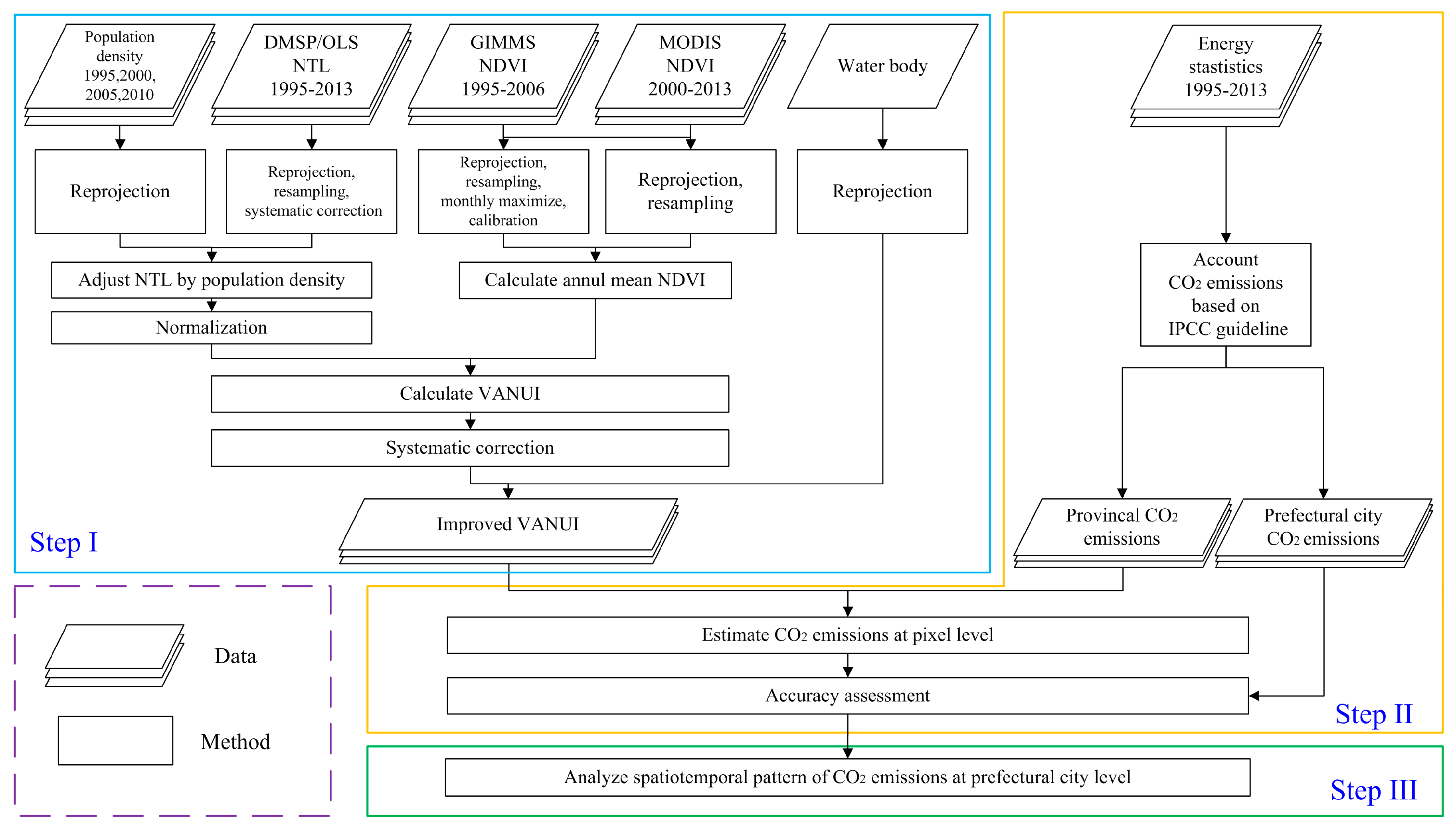
Figure 3.
Monthly GIMMS NDVI and MODIS NDVI in China from 2000–2006.
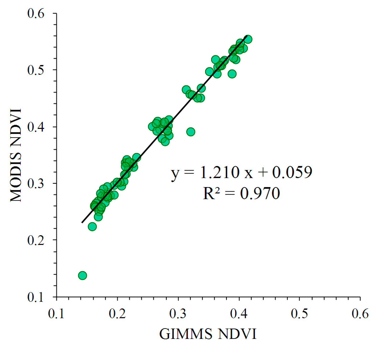
Figure 4.
Performance test of improved VANUI. (a) A false color composite of normalized NTL, NDVI and improved VANUI in red, green and blue; normalized values of (b) NTL, (c) population-adjusted NTL, (d) original VANUI and (e) improved VANUI in a line transect in the Beijing-Tianjin-Tangshan metropolitan area in 2013.
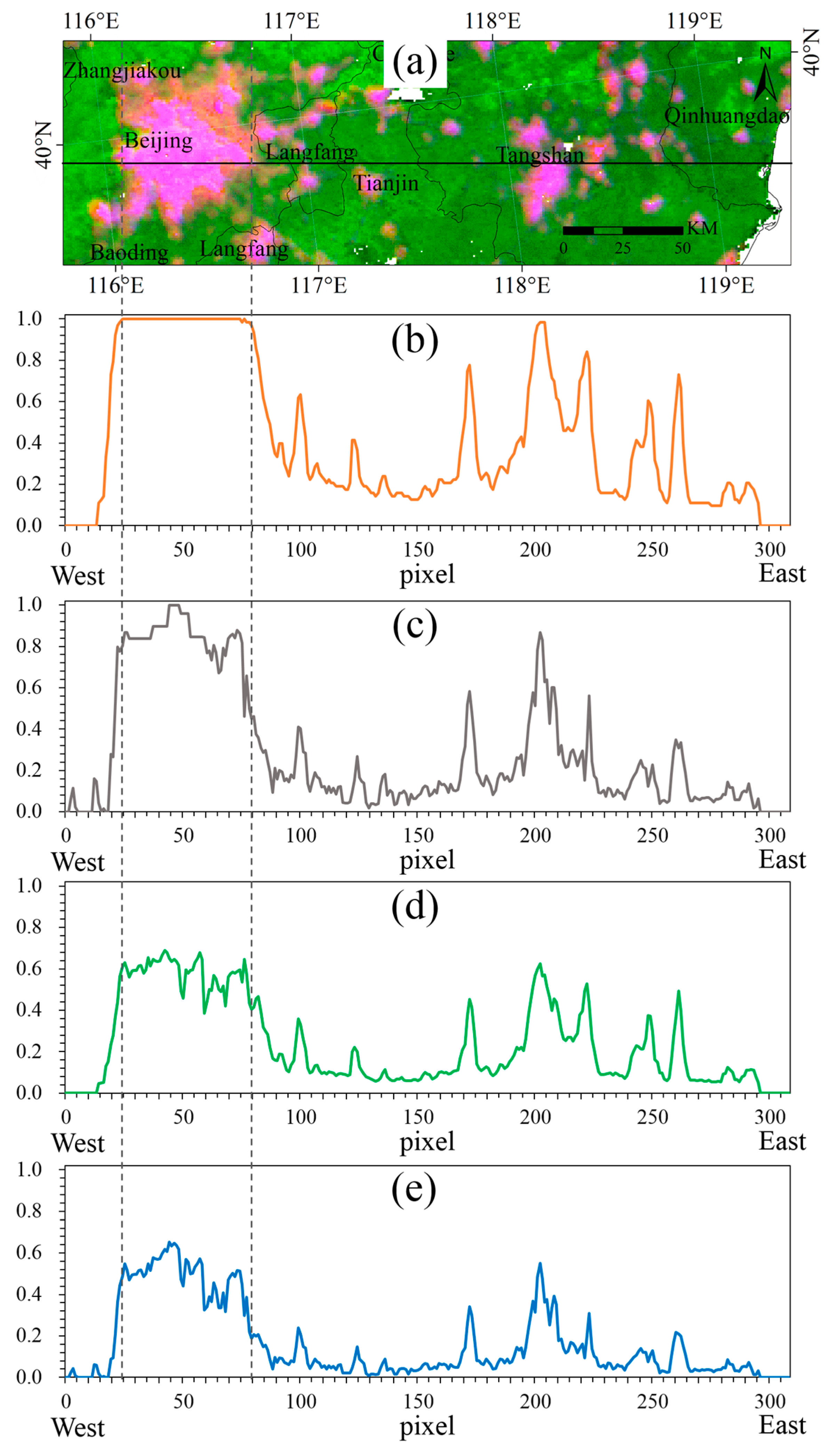
Figure 5.
Correlation analysis between modeled CO2 emissions and statistical CO2 emissions for 30 prefecture cities in 1995–2013. (a) Original NTL; (b) population-adjusted NTL; (c) original VANUI; (d) improved VANUI. RMSE and MRE are the root mean square error and mean relative error, respectively. Mt = million tons.
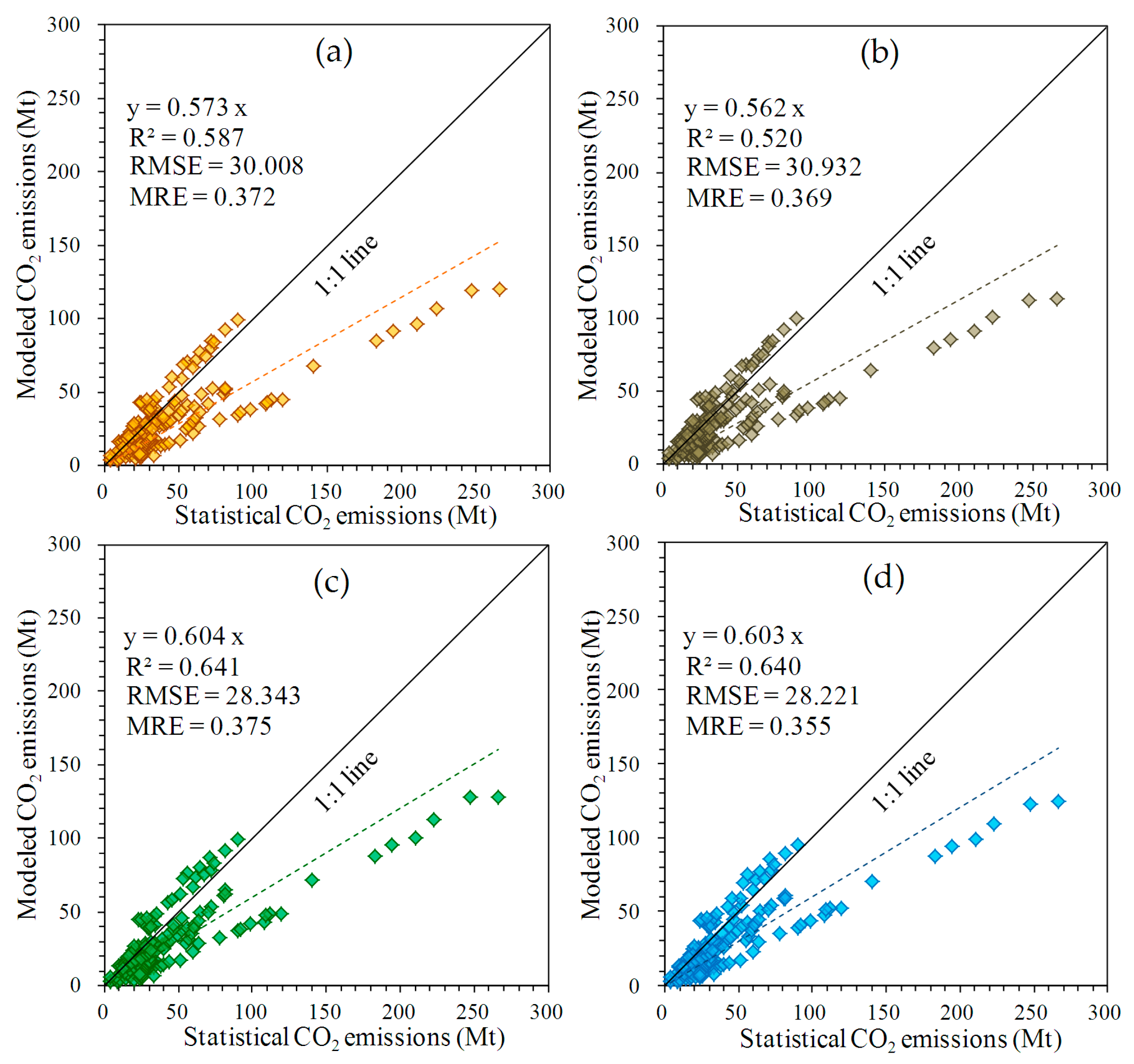
Figure 6.
Comparison of modeled CO2 emissions (CE) based on four indices in urban areas of selected cities with the Landsat 8 images in 2013 as references.
Figure 6.
Comparison of modeled CO2 emissions (CE) based on four indices in urban areas of selected cities with the Landsat 8 images in 2013 as references.

Figure 7.
Modeled pixel-level CO2 emissions in China from 1995–2013: (a) 1995; (b) 2004; (c) 2013.
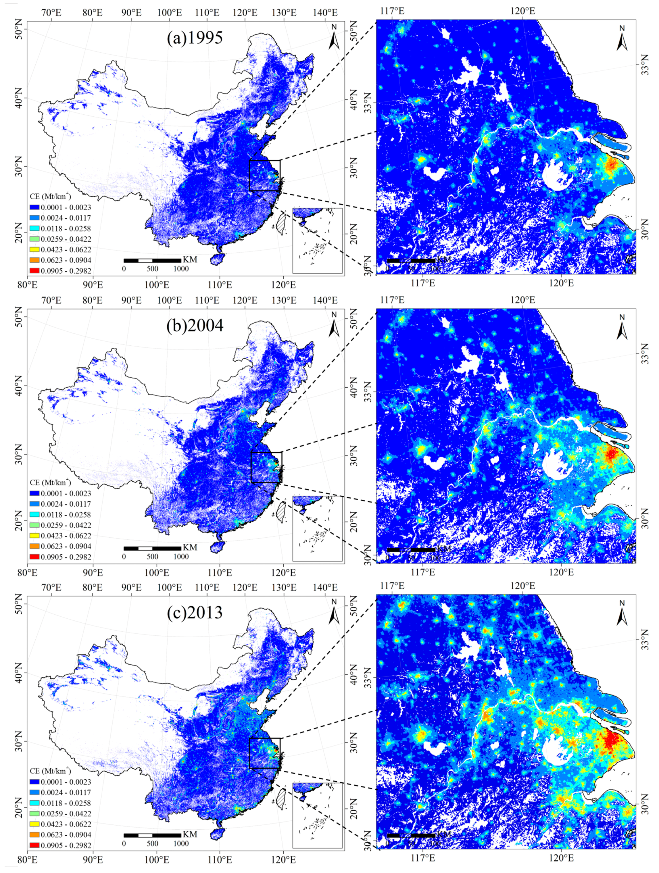
Figure 8.
Global Moran’s I of CO2 emissions in China’s prefectural cities from 1995–2013.
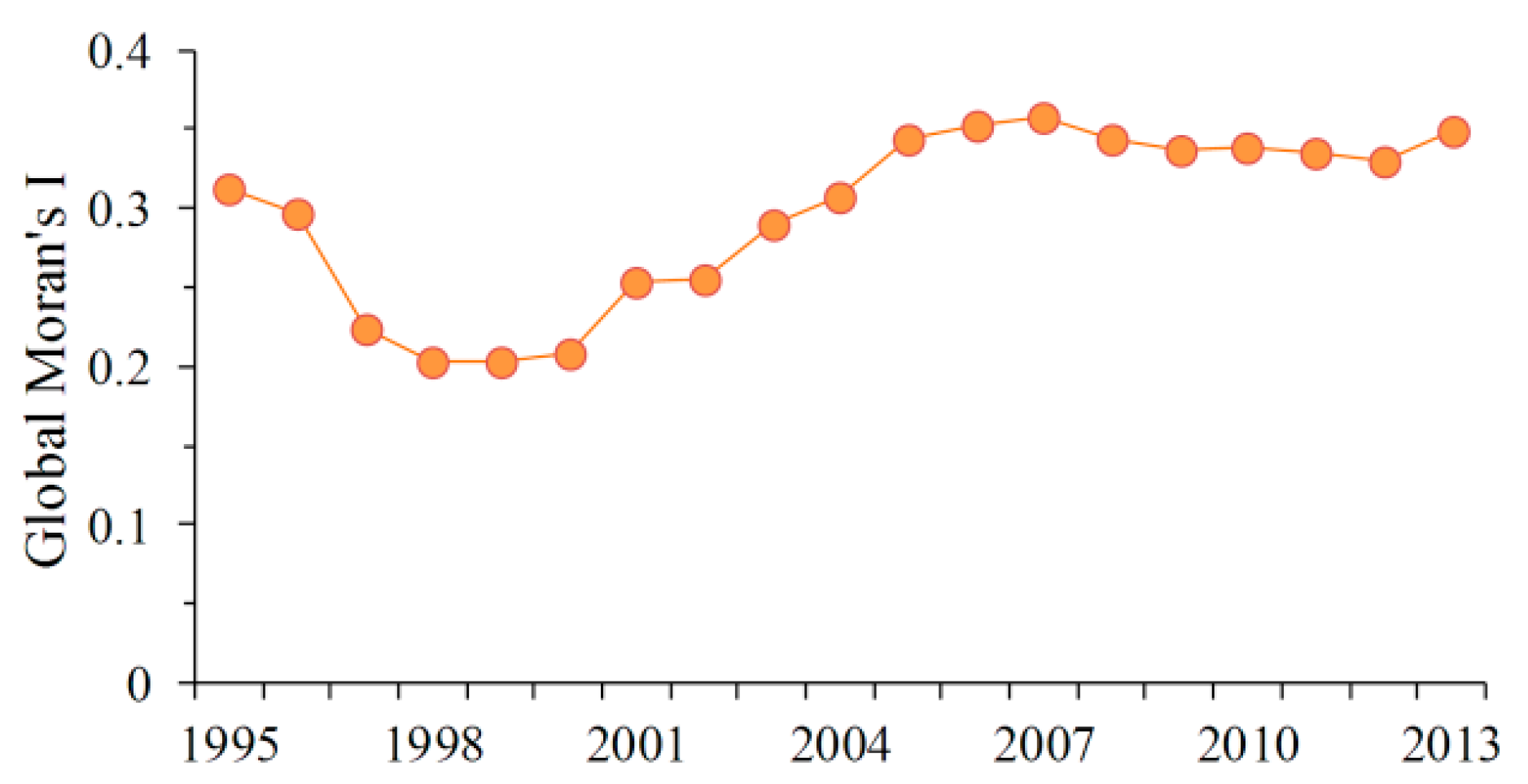
Figure 9.
Spatial dependence and heterogeneity of prefecture city level CO2 emissions. (a–d) are the spatial clusters with a 95% confidence level based on Local Moran’s I.
Figure 9.
Spatial dependence and heterogeneity of prefecture city level CO2 emissions. (a–d) are the spatial clusters with a 95% confidence level based on Local Moran’s I.

Figure 10.
Comparison between our estimation with those from literatures. CZ = Changzhou, HZ = Hangzhou, LZ = Lanzhou, NJ = Nanjing, SY = Shenyang, TJ = Tianjin, WX = Wuxi, WH = Wuhan, ZZ = Zhengzhou. Ref-1~5 refer to Wang et al. [52], Yu et al. [53], Mi et al. [54], Feng et al. [55] and Li et al. [56], respectively.


Table 1.
A summary of administrative area, population, population density and gross domestic product (GDP) for the prefectural cities with detailed energy statistics in 2013.
Table 1.
A summary of administrative area, population, population density and gross domestic product (GDP) for the prefectural cities with detailed energy statistics in 2013.
| City | Administrative Area (km2) | Population (Million) | Population Density (Persons/km2) | Gross Domestic Product (Billion RMB) |
|---|---|---|---|---|
| Changde | 18,176 | 5.80 | 319 | 2264.94 |
| Changsha | 11,816 | 7.22 | 611 | 7153.13 |
| Chenzhou | 19,342 | 4.67 | 241 | 1685.52 |
| Guangzhou | 7436 | 8.32 | 1119 | 15,420.14 |
| Hechi | 33,494 | 3.43 | 102 | 528.62 |
| Hengyang | 15,300 | 7.25 | 474 | 2169.44 |
| Hohhot | 17,344 | 3.00 | 173 | 2705.39 |
| Huaihua | 27,573 | 4.83 | 175 | 1117.67 |
| Jinan | 8177 | 7.00 | 856 | 5230.19 |
| Jincheng | 9425 | 2.30 | 244 | 1028.05 |
| Jingzhou | 14,104 | 5.74 | 407 | 1334.93 |
| Laibin | 13,386 | 2.15 | 161 | 515.57 |
| Loudi | 8110 | 3.83 | 473 | 1118.17 |
| Luoyang | 15,492 | 6.62 | 427 | 3140.76 |
| Qiqihar | 44,287 | 5.57 | 126 | 1230.40 |
| Quzhou | 8837 | 2.54 | 288 | 1056.57 |
| Shaoyang | 20,822 | 7.20 | 346 | 1130.04 |
| Shenyang | 12,980 | 7.27 | 560 | 7158.57 |
| Tangshan | 13,829 | 7.71 | 557 | 6121.21 |
| Weifang | 16,138 | 9.23 | 572 | 4420.70 |
| Xiangtan | 5005 | 2.80 | 559 | 1443.06 |
| Xiangxi | 15,470 | 2.60 | 168 | 418.94 |
| Xinyu | 3178 | 1.16 | 364 | 845.07 |
| Yichang | 21,081 | 4.10 | 194 | 2818.07 |
| Yiyang | 12,320 | 4.37 | 355 | 1123.13 |
| Yongzhou | 22,259 | 5.33 | 239 | 1175.45 |
| Yueyang | 14,858 | 5.56 | 374 | 2435.51 |
| Zhangjiajie | 9534 | 1.51 | 159 | 365.65 |
| Zhangjiakou | 36,303 | 4.41 | 122 | 1317.02 |
| Zhuzhou | 11,248 | 3.93 | 350 | 1949.43 |
Table 2.
Description of data used in this study.
| Category | Data | Description | Year | Data Source |
|---|---|---|---|---|
| Statistical data | Energy consumption | Annual consumption of raw coal, clean coal, coke, coke oven gas, crude oil, gasoline, kerosene, diesel oil, fuel oil, liquefied petroleum gases, natural gas, heat and electricity for 30 provinces and 30 prefectural-level cities | 1995–2013 | China Statistical Yearbooks Database (http://tongji.cnki.net/overseas/engnavi/navidefault.aspx) |
| Geospatial data | DMSP/OLS | Annual composite nighttime stable light data with 30 arc second grids | 1995–2013 | National Oceanic and Atmospheric Administration’s National Centers for Environmental Information (former National Geophysical Data Center) (https://ngdc.noaa.gov/eog/dmsp/downloadV4composites.html) |
| GIMMS NDVI | GIMMS 15-day composite NDVI data of China at 8-km resolution | 1995–2006 | Environmental and Ecological Science Data Center for West China (http://westdc.westgis.ac.cn/) | |
| MODIS NDVI | MODIS monthly composite NDVI data of China with 1-km resolution | 2000–2013 | International Scientific & Technical Data Mirror Site, Computer Network Information Center (http://www.gscloud.cn) | |
| Population density | Population density per 1 km of China | 1995, 2000, 2005, and 2010 | Resources and Environmental Sciences Data Center (http://www.resdc.cn) | |
| Water-masked map | A shapefile of water bodies in China | 2013 | ESRI Baruch Geoportal (https://www.baruch.cuny.edu/confluence/display/geoportal/Datasets) | |
| Administrative boundaries | Shapefiles of province and prefectural-level cities in China | 2012 | Resources and Environmental Sciences Data Center (http://www.resdc.cn) | |
| Landsat 8 OLI-TIRS | Four images covering Beijing, Shanghai, Guangzhou and Urumqi at 30-m resolution | 2013 | International Scientific & Technical Data Mirror Site, Computer Network Information Center (http://www.gscloud.cn) |
Table 3.
Parameters for accounting CO2 emissions from energy consumption in China. CR, carbon oxidation ratio.
Table 3.
Parameters for accounting CO2 emissions from energy consumption in China. CR, carbon oxidation ratio.
| Energy Type (k) | Low Calorific Value (LC, kJ/kg; kJ/m3) | Carbon Content (CC, kg/GJ) | Carbon Oxidation Factor (CR, %) | CO2 Emission Factor (EF, t/t; t/104 m3) |
|---|---|---|---|---|
| Raw coal | 20,908 | 26.37 | 94% | 1.90 |
| Clean coal | 26,344 | 27.40 | 94% | 2.49 |
| Coke | 28,435 | 29.50 | 93% | 2.86 |
| Coke oven gas | 16,726 | 12.10 | 98% | 0.73 |
| Crude oil | 41,816 | 20.10 | 98% | 3.02 |
| Gasoline | 43,070 | 18.90 | 98% | 2.93 |
| Kerosene | 43,070 | 19.60 | 98% | 3.03 |
| Diesel oil | 42,652 | 20.20 | 98% | 3.10 |
| Fuel oil | 41,816 | 21.10 | 98% | 3.17 |
| Liquefied petroleum gases | 50,179 | 17.20 | 99% | 3.13 |
| Natural gas | 38,931 | 15.30 | 99% | 2.16 |
| Heat | \ | \ | \ | 0.12 (t/GJ) |
| Electricity | \ | \ | \ | 1.01 (t/MWh) |
Table 4.
Results of statistical CO2 emissions and improved VANUI linear regressions.
| Year | T-Value of | T-Value of | R2 | ||
|---|---|---|---|---|---|
| 1995 | 39.3528 ** | 4.4998 | 0.0612 ** | 8.9893 | 0.7566 |
| 1996 | 42.2589 ** | 4.9570 | 0.0599 ** | 9.1793 | 0.7642 |
| 1997 | 45.2605 ** | 5.4585 | 0.0590 ** | 9.2259 | 0.7525 |
| 1998 | 44.2361 ** | 5.3296 | 0.0602 ** | 9.5906 | 0.7666 |
| 1999 | 43.9072 ** | 5.3252 | 0.0603 ** | 9.9401 | 0.7792 |
| 2000 | 44.9229 ** | 5.1266 | 0.0635 ** | 10.1248 | 0.7855 |
| 2001 | 40.2911 ** | 4.8998 | 0.0700 ** | 12.8600 | 0.8552 |
| 2002 | 46.8830 ** | 5.1477 | 0.0680 ** | 11.8764 | 0.8344 |
| 2003 | 48.9646 ** | 4.5677 | 0.0718 ** | 11.6740 | 0.8296 |
| 2004 | 51.8829 ** | 4.4405 | 0.0790 ** | 12.6101 | 0.8503 |
| 2005 | 39.9260 ** | 2.8469 | 0.0989 ** | 14.1337 | 0.8771 |
| 2006 | 43.8580 ** | 2.8240 | 0.1061 ** | 14.3041 | 0.8796 |
| 2007 | 45.4787 * | 2.5905 | 0.1176 ** | 14.2543 | 0.8789 |
| 2008 | 48.8460 * | 2.4972 | 0.1225 ** | 13.6811 | 0.8699 |
| 2009 | 55.0179 * | 2.4996 | 0.1259 ** | 12.7556 | 0.8532 |
| 2010 | 50.0169 * | 2.1165 | 0.1353 ** | 12.5029 | 0.8481 |
| 2011 | 55.1558 * | 2.0569 | 0.1431 ** | 12.3903 | 0.8457 |
| 2012 | 55.8876 * | 2.1275 | 0.1402 ** | 12.7299 | 0.8527 |
| 2013 | 65.4914 * | 2.3874 | 0.1333 ** | 11.5752 | 0.8271 |
Note: * and ** indicate significant at the 5% and 1% level, respectively.
© 2017 by the authors. Licensee MDPI, Basel, Switzerland. This article is an open access article distributed under the terms and conditions of the Creative Commons Attribution (CC BY) license (http://creativecommons.org/licenses/by/4.0/).
Share and Cite
MDPI and ACS Style
Meng, X.; Han, J.; Huang, C. An Improved Vegetation Adjusted Nighttime Light Urban Index and Its Application in Quantifying Spatiotemporal Dynamics of Carbon Emissions in China. Remote Sens. 2017, 9, 829. https://doi.org/10.3390/rs9080829
AMA Style
Meng X, Han J, Huang C. An Improved Vegetation Adjusted Nighttime Light Urban Index and Its Application in Quantifying Spatiotemporal Dynamics of Carbon Emissions in China. Remote Sensing. 2017; 9(8):829. https://doi.org/10.3390/rs9080829
Chicago/Turabian StyleMeng, Xing, Ji Han, and Cheng Huang. 2017. "An Improved Vegetation Adjusted Nighttime Light Urban Index and Its Application in Quantifying Spatiotemporal Dynamics of Carbon Emissions in China" Remote Sensing 9, no. 8: 829. https://doi.org/10.3390/rs9080829
Note that from the first issue of 2016, this journal uses article numbers instead of page numbers. See further details here.