Mapping Annual Riparian Water Use Based on the Single-Satellite-Scene Approach


1
Department of Biosystems & Agricultural Engineering, Oklahoma State University, Stillwater, OK 74078, USA
2
Utah Water Research Laboratory, Utah State University, Logan, UT 84321, USA
*
Author to whom correspondence should be addressed.
Remote Sens. 2017, 9(8), 832; https://doi.org/10.3390/rs9080832
Submission received: 13 June 2017
/
Revised: 4 August 2017
/
Accepted: 9 August 2017
/
Published: 12 August 2017
(This article belongs to the Section Remote Sensing in Agriculture and Vegetation)
Abstract
:The accurate estimation of water use by groundwater-dependent riparian vegetation is of great importance to sustainable water resource management in arid/semi-arid regions. Remote sensing methods can be effective in this regard, as they capture the inherent spatial variability in riparian ecosystems. The single-satellite-scene (SSS) method uses a derivation of the Normalized Difference Vegetation Index (NDVI) from a single space-borne image during the peak growing season and minimal ground-based meteorological data to estimate the annual riparian water use on a distributed basis. This method was applied to a riparian ecosystem dominated by tamarisk along a section of the lower Colorado River in southern California. The results were compared against the estimates of a previously validated remotely sensed energy balance model for the year 2008 at two different spatial scales. A pixel-wide comparison showed good correlation (R2 = 0.86), with a mean residual error of less than 104 mm∙year−1 (18%). This error reduced to less than 95 mm∙year−1 (15%) when larger areas were used in comparisons. In addition, the accuracy improved significantly when areas with no and low vegetation cover were excluded from the analysis. The SSS method was then applied to estimate the riparian water use for a 23-year period (1988–2010). The average annual water use over this period was 748 mm∙year−1 for the entire study area, with large spatial variability depending on vegetation density. Comparisons with two independent water use estimates showed significant differences. The MODIS evapotranspiration product (MOD16) was 82% smaller, and the crop-coefficient approach employed by the US Bureau of Reclamation was 96% larger, than that from the SSS method on average.
1. Introduction
Large extents of the Colorado River floodplain are currently occupied by invasive species, such as tamarisk or salt cedar (Tamarix spp.) and Russian olive (Eleagnus angustifolia), that have replaced the native species, such as cottonwood (Populus spp.) and willow (Salix spp.). Tamarisk, in particular, has invaded millions of hectares of riparian floodplain in western U.S. [1], particularly in the dry southwestern states of Arizona, New Mexico, Texas, Nevada, Utah, and California [2]. Glenn and Nagler [3] reported that tamarisk spreads at rates exceeding 20 km∙year−1, becoming a dominant plant on the banks of rivers, streams, and ponds from eastern Oklahoma to northwestern California, and from western Montana to Sonora, Mexico. In addition, tamarisk has a high tolerance to salinity [4,5] and drought [6]. The negative impacts of tamarisk invasion include, but are not limited to: displacing native vegetation [3,7], increasing fire frequency [8], degrading wildlife habitat [9], reducing biodiversity [10], and increasing water consumption [2,11]. The impact of tamarisk on water availability has been the subject of numerous studies, such as the one by Zavaleta [2], who reported that the financial burden of high tamarisk water use on water supplies, hydropower generation, and flood control could reach $285 million U.S. dollars per year. Other researchers have found lower rates of tamarisk water use [12,13,14]. Since millions of dollars are spent annually on removal and restoration projects, it is crucial for decision-makers and water managers, especially in water-scarce areas, to have access to tools that can provide accurate estimates of water use by invasive species with reasonable financial, computational, and human resources requirements.
Among the different methods available for quantifying riparian water use, remote sensing approaches have the advantage of capturing the high spatial variability common in riparian ecosystems. Existing methods for the remote sensing of riparian water use or evapotranspiration (ET) can be broadly grouped into two major categories: empirical approaches based on vegetation indices (VI); and physically based, remotely sensed energy balance (RSEB) models. The RSEB models rely on land surface temperature derived from the thermal bands of air- and space-borne imagery to compute ET as the residual of the surface energy balance. On the other hand, VI approaches are based on the plant-specific relationships between VIs and ET. An advantage of the RSEB models is their potential to detect variations in ET caused by short-term environmental stressors (due to the use of land surface temperature), while VI approaches may fail to do so unless the suboptimal conditions last long enough to affect biomass [13,15]. Another advantage is that RSEB models can be applied over diverse climatic conditions and ecosystems [16]. In contrast, VI approaches may not be easily transferred to geographic areas different from the one where they were developed [12]. On the other hand, RSEB models require numerous inputs [17] and depend on a complex iterative process to accurately compute surface energy balance components [18,19,20]. The iterative process requires selection of end-member pixels with a manual checkup by an experienced operator to ensure the calibration accuracy [18], and to minimize the constraints associated with directional radiometric surface temperature or vegetation fraction cover [17]. An additional challenge in validating the RSEB models with ground-based measurements is the closure of energy balance, which may not be achieved [17,20]. The VI approaches benefit from significantly smaller computational costs to run. As a result, they are usually preferred in studying inter-annual variations of ET across a region with similar hydro-climatic conditions, providing similar levels of uncertainty compared to RSEB models [20,21,22].
The RSEB models have been implemented before to estimate riparian ET at the Middle Rio Grande Basin in New Mexico [23], along the North Plate River in the Nebraska Panhandle [24], over the Lower Virgin River in Nevada [25], and along the Lower Colorado River in southern California [14]. Multiple VI-based approaches have also been developed and applied to estimate riparian ET. For example, the Modified Soil Adjusted Vegetation Index (MSAVI: [26]) has been empirically related to ET from groundwater-dependent riparian vegetation [27]. The Enhanced Vegetation Index (EVI: [28]) derived from Moderate Resolution Imaging Spectroradiometer (MODIS) has been also used in several previous studies [12,15,16,29,30]. Nagler et al. [15,31] developed a method to compute riparian ET using MODIS-EVI and maximum daily air temperature (Tair), and reported an error of ±25% when compared with flux tower observations from three western U.S. river corridors. This empirical relationship was modified by [16], showing the potential application of MODIS land-surface temperature instead of ground-based maximum Tair. Later, [32] developed a new linear relation between scaled EVI from MODIS and the Blaney–Criddle reference ET (ETo-BC: [33]). This new model had reduced error (within 20%) when applied to riparian and agricultural areas along the Lower Colorado River in the southwestern U.S. In a more recent study, [29] replaced ETo-BC with the Penman–Monteith ETo [34], and developed an exponential relation. This newer method had a better performance in predicting ET, with an error of 10% when compared with flux tower and water balance data from riparian zones and irrigation districts at multiple locations from western U.S., Spain, and Australia [29].
Among all VI approaches developed in the past, the single-satellite-scene (SSS) method developed by [35,36] has the least computational costs, as it requires only one image during peak vegetation growth to map the annual riparian ET. The SSS method relies on Normalized Difference Vegetation Index (NDVI) estimates, scaled from zero to one using two NDVI extremes representing zero and full-cover vegetation obtained from within the selected scene. The scaled NDVI was found to be highly correlated with riparian ET estimates from flux towers in California, Colorado, and New Mexico, with errors between −45 and 40 mm∙year−1 (less than 13%) [35]. Similar errors were reported when Landsat derived EVI was used in the SSS method [37]. This method has been also applied to study ET and groundwater dynamics [38,39], a cost/benefit analysis of tamarisk control [40], the sustainability of vegetation, hydrology, and habitat value [41], tamarisk leaf beetles’ impact on water availability [42], and impacts of Colorado River delta pulse flow on riparian water use [43]. To the best of our knowledge, no independent study has assessed the performance of the SSS method in the past. Considering the potential of this method, evaluating its performance under variable hydro-ecological conditions would be beneficial to water managers and other potential users. The main objective of this study was to evaluate the performance of the SSS method using previously validated RSEB results, and to apply it over a 23-year period (1988–2010) to investigate inter-annual riparian ET variations across parts of the Cibola National Wildlife Refuge in the Lower Colorado River Basin.
2. Materials and Methods
2.1. Study Area
The study area included parts of the Cibola National Wildlife Refuge (CNWR), which occupies about 70 square kilometers in the floodplains of the lower Colorado River, about 150 river km downstream of the Parker Dam. The CNWR was established in 1964 by the U.S. Bureau of Reclamation (USBR) to serve as a refuge and breeding area for migratory birds and wildlife, and to mitigate flooding by the Colorado River. The average annual rainfall is less than 100 mm in this low-desert environment [13]. Most of the rainfall occurs in July and August with occasional winter rains. The average air temperature ranges from 4.0 °C in December to 38.0 °C in August [13]. More than 90% of CNWR is covered by tamarisk (Tamarix spp.), followed by mesquite (Prosopis velutina), cottonwood, willow, arrowweed (Pluchea sericea), qualibush, and fourwing saltbush [13,14].
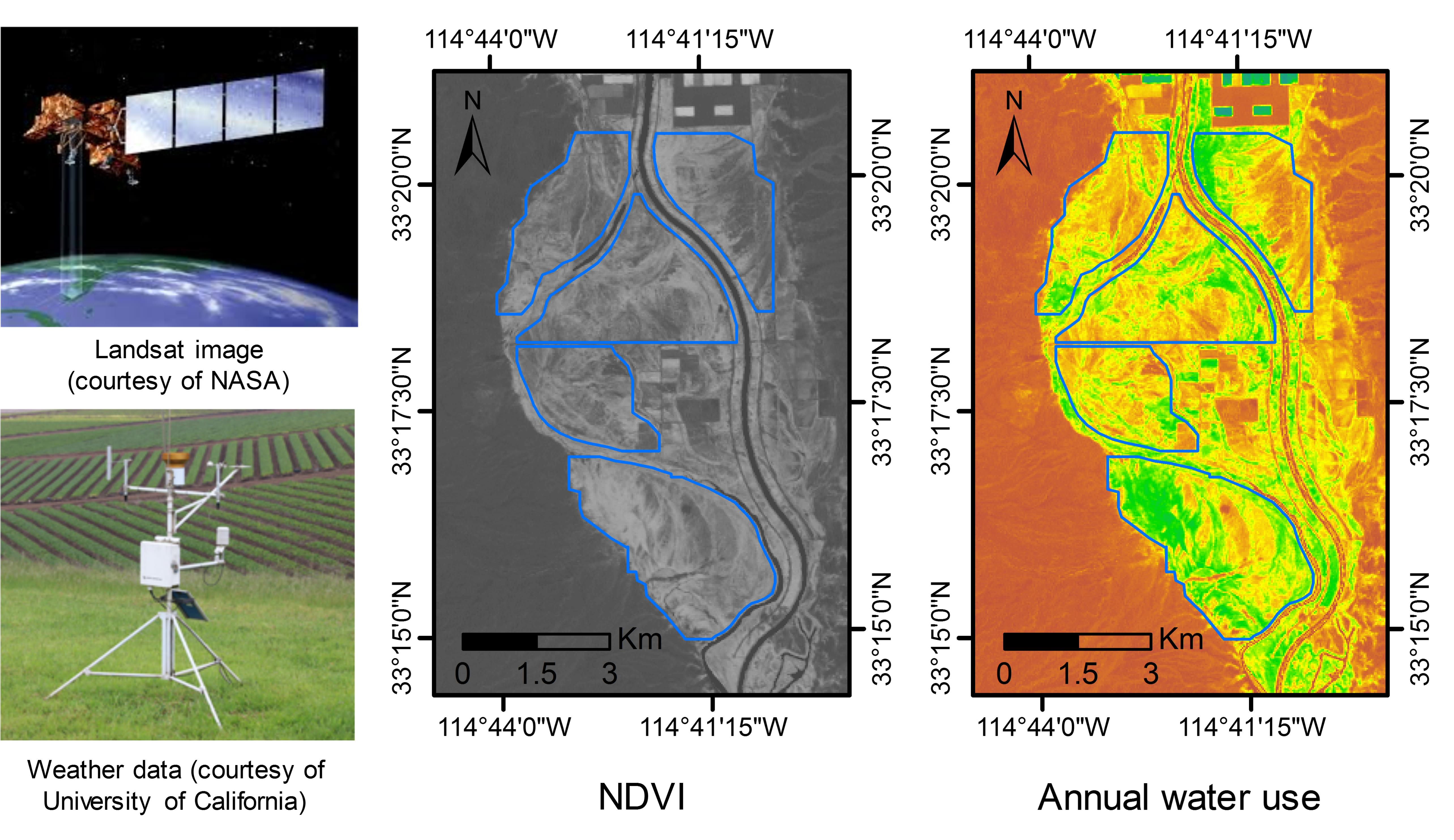
The location of the study area within the Colorado River basin is presented in Figure 1 (left panel). The new and old Colorado River channels are specified in the satellite image (right panel) along with six subareas used in analyzing ET signals in this study. The old river channel serves as the border between California (CA) and Arizona (AZ). Subareas 2, 3, and 4 are located in AZ, while subareas 1, 5, and 6 are in CA. Since 1964, when most of the river flow was diverted to the new channel, the old channel has been carrying agricultural return flows from the Palo Verde Irrigation District (PVID) upstream of CNWR, as well as a small, regulated flow to support the wildlife.
2.2. Single-Satellite-Scene (SSS) Apporach
The Single-Satellite-Scene (SSS) is a simple method of estimating annual riparian ET based on just one mid-summer satellite image and some ground-based meteorological data [35,36]. In this method, the annual riparian ET is a function of NDVI*, reference ET (ETo), and precipitation as:
where NDVI* is a scaled NDVI, computed using the relationship presented in [36] as:
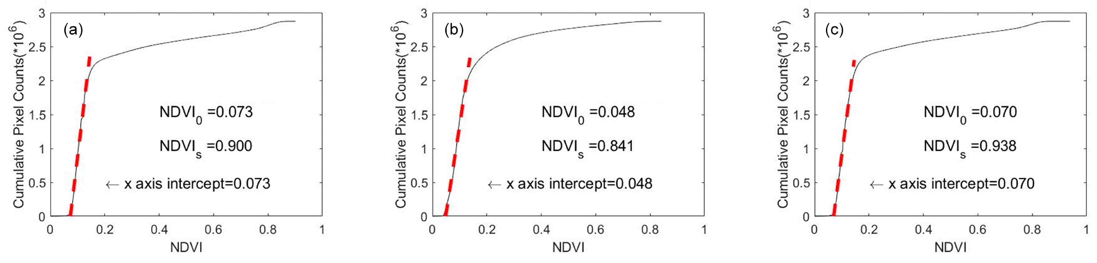
where NDVIo is NDVI at zero vegetation cover and NDVIs is NDVI at saturation, both extracted from the same satellite scene to be used in ET estimation. The conversion of NDVI to NDVI* is performed to remove the variations inherent in this parameter caused by atmospheric, soil, and vegetation factors [36,44,45], making it possible to use NDVI estimated by different sensors at different times and locations. The selection of NDVIo and NDVIs is a critical step. These parameters are estimated by developing a cumulative frequency distribution graph of NDVI values for the selected scene [36]. At the low end of this graph, the relationship (NDVI vs. cumulative pixel count) becomes asymptotic and choosing an appropriate NDVIo becomes subjective [36]. To minimize such subjectivity, a line is fitted to the near-linear lower portion of the NDVI cumulative frequency distribution and the x-intercept of the fitted line is taken as NDVIo. NDVIs is chosen from a region with the maximum possible NDVI (e.g., irrigated crops with full-cover or thick riparian forests). Further details of this method are presented in [35] and [36]. The main assumptions of the SSS method are the presence of shallow groundwater, arid/semi-arid environments, and similar conditions before and after (homeostasis) the mid-summer satellite image [35].
ET = (ETo − Precipitation) × NDVI* + Precipitation
NDVI* = (NDVI − NDVIo)/(NDVIs − NDVIo)
A major question for potential users of the SSS method could be the selection of the single scene to be used in the analysis. The sensitivity of estimated annual riparian ET to the selected image was investigated by applying the method to three Landsat images from mid-summer 2008. The three NDVI maps used in this study were processed by the Landsat Ecosystem Disturbance Adaptive Processing System (LEDAPS) [46], which applies the Second Simulation of a Satellite Signal in the Solar Spectrum (6S) radiative transfer models to minimize the radiometric errors. The performance of the SSS method was then assessed on a distributed basis through comparing its result with that obtained from a previously validated remotely sensed energy balance (RSEB) model. This RSEB model was a modified Surface Energy Balance Algorithm for Land (SEBAL) model [14]. SEBAL has been extensively validated before under variable land covers and hydro-climatic settings [47,48]. The land surface energy balance components considered in SEBAL are presented in Equation (3), assuming energy consumed in photosynthesis and energy stored in the canopy are insignificant.
where LE is the latent heat flux, and is estimated as a residual of net radiation (Rn), soil heat flux (G), and sensible heat flux (H). The LE estimated based on Equation (3) represents the instantaneous flux at the time of satellite overpass. Extrapolation of this instantaneous flux to daily ET in SEBAL is accomplished by using evaporative fraction (EF), estimated as the ratio of instantaneous LE to instantaneous available energy (Rn − G). Instantaneous EF is assumed to be the same as the 24-h (daily) EF, representing the ratio of daily LE to Rn [47,49]. Details on the computational steps of SEBAL are presented in [47].
LE = Rn − G − H
Taghvaeian et al. [14] applied the modified SEBAL model over the study area (CNWR), using 21 Landsat TM images acquired in 2008. In the modified SEBAL application at CNWR, an adjustment coefficient was adopted to account for the canopy temperature contamination caused by shadows of tall riparian vegetation [14]. The results were compared against the estimates of two independent methods: the Bowen ratio flux tower and the White method, which is based on the diurnal fluctuations of groundwater [50]. On a seasonal basis, ET estimates of the modified SEBAL were within 2% and 10% of those from the White method and Bowen ratio, respectively [14]. This difference was less than the expected error of each method, giving confidence to the accuracy of this RSEB model. Hence, the modified SEBAL was used as the reference to evaluate the performance of the SSS method.
Comparisons were made at two scales: pixel-based and area-wide. At the pixel-based scale, ET values were extracted for each method using a randomly scattered collection of 1571 circular sampling features with a diameter of 120 m. At the area-wide scale, comparisons were made for the six subareas demonstrated in Figure 1, with average and total areas of 5.12 and 30.74 km2, respectively. After obtaining the ET data from each method, the residual and percent error were calculated as:
where SSS-ET is the ET estimated by the SSS method, and RSEB-ET is the ET from the modified SEBAL model.
Residual error = SSS-ET − RSEB-ET
2.3. Long-Term Estimates
After evaluating the performance of the SSS method, long-term ET estimates were obtained over a 23-year period from 1988 to 2010. The meteorological data were obtained from the Palo Verde weather station, which is operated and maintained by the California Irrigation Management Information System (CIMIS). This weather station is located about 4.5 km north of the study area, and is the closest weather station in the region. A mid-summer Landsat image was selected in each study year and used for computing NDVIo, NDVIs, and NDVI*, which was integrated with annual grass-based reference ET (ETo) [51] and precipitation to map annual riparian ET based on Equation (1). The average annual ET was estimated for the subareas in CA (1, 5, 6) and the subareas in AZ (2, 3, 4), and was compared with two independent ET estimates: the remotely sensed MODIS ET product known as MOD16 [52,53] averaged over the same subareas, and the crop-coefficient approach implemented by USBR in the Lower Colorado River Accounting System (LCRAS) and reported for the CA and AZ sections of the study area.
The MOD16-ET was downloaded from the University of Montana’s Numerical Terradynamic Simulation Group data archive (http://www.ntsg.umt.edu). The MOD16 global ET dataset is primarily based on the Penman–Montheith equation [52,53,54], and has a spatial resolution of 1.0 km. Although this resolution was much coarser than the resolution of the SSS estimates used in this study, MOD16 was included in the comparison because it is available to water managers at no cost. A comparison of the MOD16-ET and the SSS-ET was made only for the 11-year period of 2000 to 2010 due to the unavailability of MOD16 before the year 2000.
In the USBR LCRAS approach, daily riparian ET is estimated as a product of ETo and crop coefficients (Kc) and summed to obtain the annual ET. Climatological data from the California Irrigation Management Information System (CIMIS) and the Arizona Meteorological Network (AZMET) are used for these ET estimations. The details on ET estimation methods and procedures, as well as annual riparian ET from the CA and AZ areas of CNWR, are presented in the LCRAS reports [55,56]. For comparison with SSS estimation, LCRAS-ET estimates in acre-feet were divided by the CNWR area at each state (provided in the same report) to obtain the annual ET in units of water depth. The spatial extent of the CA and AZ regions in the LCRAS and SSS methods were not exactly the same, but similar enough to warrant a comparison between the two approaches. The LCRAS reports are available from 1995 to 2011. However, to be consistent with MOD16 data, a LCRAS–SSS comparison was conducted for the period from 2000 to 2010.
3. Results and Discussion
3.1. SSS Evaluation
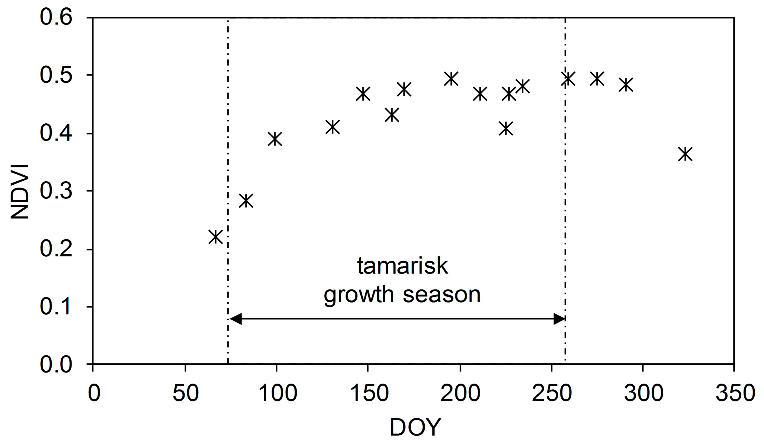
The SSS method requires only a single satellite image during peak riparian growth to estimate ET. Figure 2 demonstrates the evolution of NDVI, averaged over the study area, for all cloud-free Landsat TM5 scenes acquired in 2008. The average NDVI varied from 0.22 in March to 0.49 in September. The maximum NDVI over the CNWR occurred during summer, with the highest values of 0.49, 0.47, and 0.49 observed on day of year (DOY) 195 (13 July), 227 (14 August), and 259 (15 September), respectively. To examine the sensitivity of the SSS method to the selection of a Landsat scene, each of these three dates was used separately in estimation of the annual ET.
The selection of NDVIo and NDVIs for each of the three scenes was facilitated by plotting cumulative NDVI frequency graphs with the x-intercept (NDVIo) of the fitted line to the near-linear lower portion of the cumulative frequency graph and the maximum possible NDVI (NDVIs). The NDVIo was 0.07, 0.05, and 0.07, for DOYs 195, 227, and 259, respectively, and the NDVIs was 0.90, 0.84, and 0.94 for the same DOYs (Figure 3). This information was used in mapping NDVI* and eventually the SSS-ET. The annual SSS-ET averaged over the entire study area was 677, 676, and 658 mm∙year−1 for DOYs 195, 227, and 259, respectively. The average annual RSEB-ET was smaller, at 571 mm∙year−1.
For the pixel-based evaluation, both the SSS-ET and RSEB-ET estimates were extracted using 1571 randomly located samples. In general, the pixel-based comparison showed good correlation between the two methods, with a coefficient of determination (R2) larger than 0.86. The residual error varied between 84 and 104 mm∙year−1 for the three DOYs (Table 1). This translated to percent errors from 14.3 to 17.7%. Figure 4 demonstrates a scatterplot of ET estimates and how they populate around the 1:1 line. Two distinct areas can be observed in the scatterplot with higher densities of points. The majority of points in the lower-left cluster in Figure 4 were from subareas 1, 2, and 3, where vegetation was sparse, with average NDVI less than 0.31 for all three DOYs. The overestimation of the SSS-ET over the low-vegetation areas (lower-left cluster in Figure 4) can be attributed to the inclusion/exclusion of surface temperature in the RSEB model and SSS method. Due to the exclusion of surface temperature, the reduced ET from the low vegetation and bare soil is not fully accounted for by the SSS method. However, a minimum NDVI threshold can be set based on local vegetation and weather data to minimize the errors while applying the SSS method under low-vegetation conditions. The higher ET cluster mostly contained samples from subareas 4, 5, and 6, with average NDVI ranging from 0.37 to 0.55.
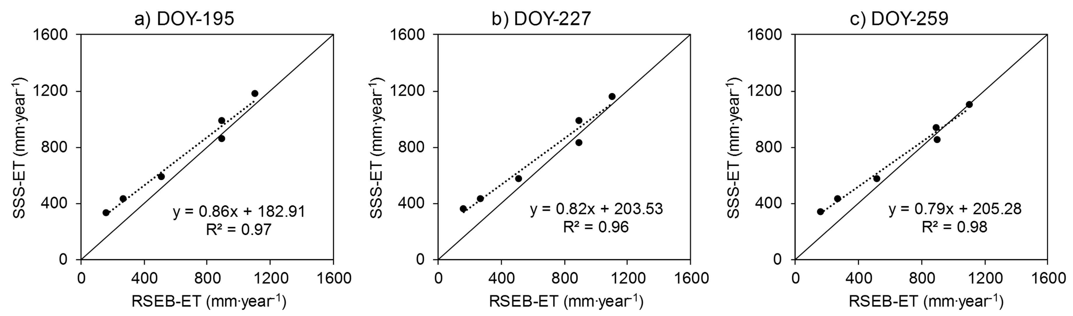
The evaluation of SSS performance was also conducted at the area-wide scale, where a comparison of the SSS-ET and RSEB-ET was made on all DOYs (195, 227, 259) over the six subareas within the CNWR. The reason behind performing an area-wide comparison was that the SSS method will most likely be implemented by water managers to obtain estimates over larger areas and to use the information in making decisions, as opposed to research applications that may require more details. Similar to the pixel-based comparison, the area-wide results had good agreement (R2 ≥0.96) with RSEB-ET estimates (Figure 5). The residual errors were smaller at 95, 90, and 71 mm∙year−1 for DOYs 195, 227, and 259, respectively. The percent errors were 14.9, 14.1, and 11.1% for the same DOYs, respectively.
The percent errors found in this study for the pixel-based (<17.7%) and area-wide (<14.9%) comparisons are promising, since they are within typical ranges of errors in the measurements of other water balance components in riparian ecosystems. These errors are also close to the lower end of errors of VI approaches, which typically range from 15% to 40% [57] depending on the knowledge and experience of an operator. Based on this metric, the estimated error of the SSS method is acceptable considering the fact that it requires minimal operator knowledge and that the entire process can be automated using computer programming.
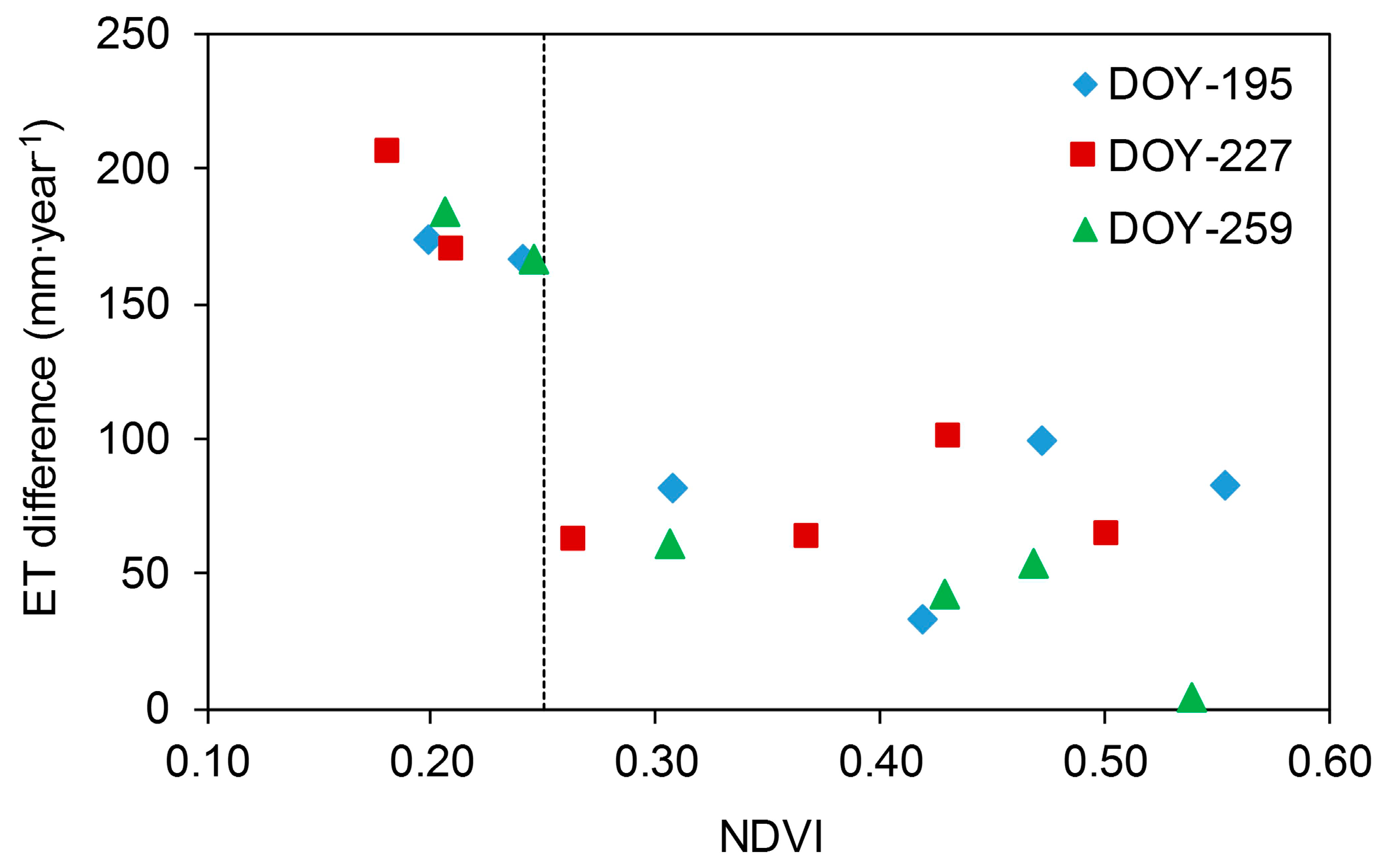
The area-wide comparison revealed a potential relationship between the magnitude of SSS-ET error and the vegetation density. The greatest difference between the two methods was 206 mm∙year−1 from subarea 3 for DOY 227. This subarea had the smallest average NDVI of 0.18. In contrast, the smallest difference in annual ET estimates was 4 mm∙year−1 from subarea 5 for DOY 259. The average NDVI was 0.54 over this subarea. To further investigate this relationship, the differences between the SSS-ET and RSEB-ET were plotted against the average NDVI of each subarea (Figure 6). The differences were greatest for NDVI values smaller than 0.25, but were reduced significantly and remained insensitive beyond this NDVI threshold. Subareas 1 and 3 had average NDVI values less than 0.25 for all three DOYs. Removing these subareas from the analysis resulted in a significant reduction in average residual errors to 58, 42, and 20 mm∙year−1 for DOYs 195, 227, and 259, respectively. The percent errors were also smaller, at 6.8%, 5.0%, and 2.4% for the same DOYs, respectively. The inverse relationship between the SSS-ET error and NDVI is expected, as this method was developed and calibrated to estimate the water use of riparian species. Thus, it underperforms over bare soil and low-vegetation areas.
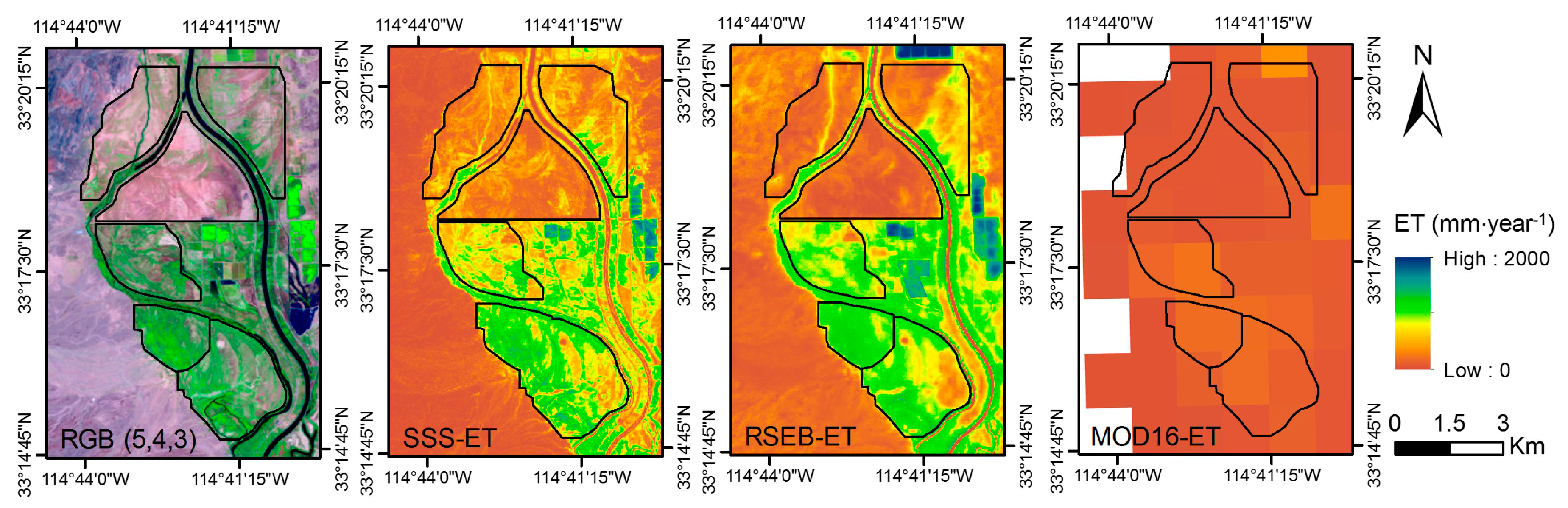
No significant differences in SSS-ET estimates were found among the three selected scenes, and all performed satisfactorily based on acceptable errors for VI approaches. The Landsat image of 17 August (DOY 227) was selected for the annual ET estimation for the validation year 2008. Previous studies [35,58,59] have suggested June to August as a representative period to characterize peak biomass and water use of riparian vegetation in western U.S. A visual representation of annual ET estimated by SSS, RSEB, and MOD16 for the year 2008 is shown in Figure 7. Missing pixels in the MOD16 map represent barren or sparsely vegetated areas where ET values are not estimated.
3.2. Inter-Annual Variation of Water Use
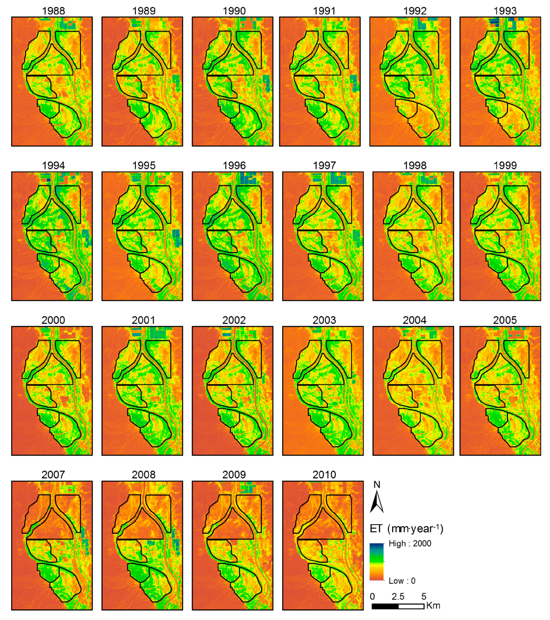
Annual riparian water use was mapped over the study area for a 23-year period from 1988 to 2010, after the selection of an appropriate mid-summer Landsat image. For most of the studied years (18 out of 23), the selected scene was from August, and the remaining scenes were from July and September. The procedure explained in previous sections was followed for estimating NDVIo and NDVIs. NDVIo had a range of 0.06 to 0.10, and NDVIs varied between 0.83 and 1.0 (Table 2). Comparatively, lower variation (0.04) was observed in NDVIo than in NDVIs (0.17). The reference ET (ETo) values were between 1644 mm∙year−1 to 2015 mm∙year−1, with an average of 1785 mm∙year−1 (Table 2). Annual precipitation varied from 1 mm∙year−1 to 177 mm∙year−1, with an average of 66 mm∙year−1 during the study period.
The long-term (1988–2010) average annual ET over the CNWR was 748 mm∙year−1, with the smallest value observed in 2010 at 483 mm∙year−1 and the largest in 1994 at 915 mm∙year−1. This annual average SSS-ET (748 mm∙year−1) was about 42% of long-term average ETo. The annual average precipitation was 66 mm∙year−1, only about 9% of the average SSS-ET during the study period. The annual ET for the year 2006 was excluded due to the violation of a major assumption in the SSS method. Based on this assumption, the conditions before and after the single satellite scene should be similar (homeostasis conditions) [35], which was not fulfilled for the year 2006 due to a massive wildfire. This wildfire, which occurred in mid-July 2006, can also explain the considerable (33%) reduction in riparian water use after 2006. The average values of SSS-ET were 754 and 508 mm∙year−1 before and after 2006, respectively. Another factor that may have played a role is the release of tamarisk leaf beetles (Diaorhabda carinulata), which started in 2001 in some riparian forests upstream of the study area [42]. Pre- and post-beetle studies in the western U.S. have reported a 50% reduction in daily midsummer ET [60] and a 16% (204 mm∙year−1) reduction on an annual basis [25]. A graphical representation of inter-annual variations of SSS-ET during the study years and the impact of the 2006 wildfire on tamarisk ET over the CNWR is shown in Figure 8.
The average annual tamarisk ET was 748 mm∙year−1. If the entire tamarisk monoculture area of 182 × 106 m2 (18,200 ha) [13] in the lower Colorado River Basin is similar to that of the CNWR, the annual water loss would be about 136.3 × 10⁶ m3 (110,514 acre-foot). This amount of water consumed by tamarisk would be less than 1.5% of the long-term (1988–2010) average annual flow (1.12 × 10¹⁰ m3) of the Colorado River measured at Lee’s Ferry, AZ and about 18% of the long-term (1991–2010) average annual water use (620,835 acre-foot: [61]) by the city of Los Angeles, CA.
The annual riparian water use estimates in this study were within the range of ET rates reported by previous studies. Ref. [12] reported annual ET from 608 to 1005 mm∙year−1, with an average of 825 mm∙year−1 from the entire CNWR during the study period 2000 to 2008 based on MODIS EVI. However, reference [62] found an average annual ET of 1110 mm∙year−1 from the CNWR for the period of 2000 to 2006. This is significantly larger (44%) than the results of this study, with a maximum annual ET of 851 mm∙year−1 during the same period. Potential reasons for the observed differences include, but are not limited to, differences in implemented methods, possible differences in the weather parameters used in analysis (weather station selected), and differences in space-born imagery. The studies by [12,62] applied MODIS imagery with a 250 m ground resolution, which can potentially include non-target or multiple land covers within a pixel [12], whereas the present study used finer resolution (30 m) Landsat imagery.
3.3. Comparisons with MOD16 and LCRAS
The comparison between SSS, MOD16, and LCRAS water use estimates was conducted for 10 years from 2000 to 2010, excluding the year 2006 due to the wildfire that occurred in the study area. The annual ET estimates from MOD16 were significantly smaller than those based on the SSS method, with a minimum and maximum of 92 and 187 mm∙year−1 during the comparison period, respectively. On average, the MOD16 estimate of riparian water use over the study area was 122 mm∙year−1 (excluding 2006), which is about 82% smaller than the average SSS-ET for the same period (674 mm∙year−1). This difference could be due to the MOD12 land cover product [63,64] used in estimating MOD16, which has a coarse spatial resolution (500 m) and classifies most of the CNWR as croplands with some open/closed shrublands. In addition, MOD16 has a spatial resolution of 1 km, much coarser than the 30 m resolution of Landsat imagery used in the SSS. This introduces a significant contamination from nearby desert areas. The finer spatial resolution of Landsat is achieved at the cost of coarser temporal resolution. Nevertheless, most riparian corridors in western U.S. are narrow in extent and do not experience rapid temporal variations. This makes Landsat a better option than MODIS when it comes to studying spatially heterogeneous riparian water consumption. The underestimation of MOD16 has been reported for croplands in previous studies [65,66,67]. The MOD16-ET from the CA portion was 34% greater than the AZ areas. Similar to the MOD16-ET, the SSS method estimated greater (24%) ET from CA.
In contrast to MOD16, the annual riparian ET estimates reported in LCRAS were greater than the SSS-ET estimates (Figure 9). The annual ET based on LCRAS varied between 787 mm∙year−1 (2010) and 1530 mm∙year−1 (2001), with an average of 1320 mm∙year−1 during the comparison period (excluding 2006). This was 96% larger than the average SSS-ET (674 mm∙year−1) during the same period. The difference between the LCRAS and SSS estimates of ET was greater than 600 mm∙year−1 for the years from 2000 to 2009. However, the difference was significantly reduced to 304 mm∙year−1 in 2010. For the year 2010, LCRAS reported an annual ET of 787 mm∙year−1, which was about 56% lower compared to the 2009 ET of 1231 mm∙year−1. This abrupt decrease can be attributed to an adjustment made in 2010 on crop coefficients (Kc), which reduced riparian ET by 30 to 40% [56]. In the original LCRAS method, the maximum Kc (mid-season stage) was 1.15 [68], which was reduced to −0.76 [69] in the 2010 estimation. The updated Kc values in LCRAS are consistent with those reported by [14] over dense tamarisk stands within the CNWR based on the RSEB model and the groundwater-based method. The overestimation error of LCRAS has been also reported in [12,13].
While both of the remotely estimated ET products (SSS and MOD16) were able to capture ET differences between CA and AZ, the Kc-based LCRAS was not able to account for those ET variations. After the wildfire of 2006, the 4-year (2007–2010) average SSS-ET from the CA portion was 60% greater compared to the AZ portion. This difference was 10% on average during the 4 years before the wildfire (2002–2005). However, the Kc-based LCRAS reported only 1% greater ET from CA after the 2006 wildfire, and no difference before the wildfire.
3.4. Impact of Wildfire on Water Use
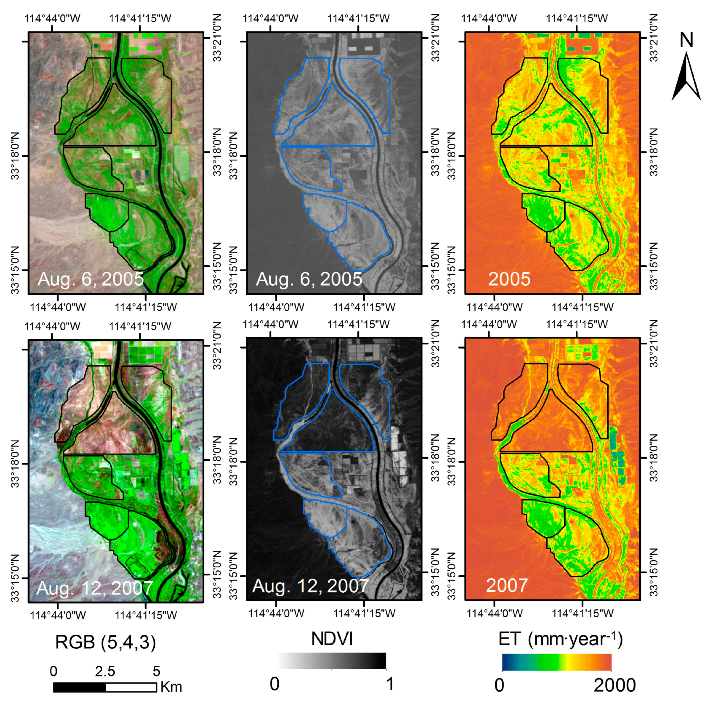
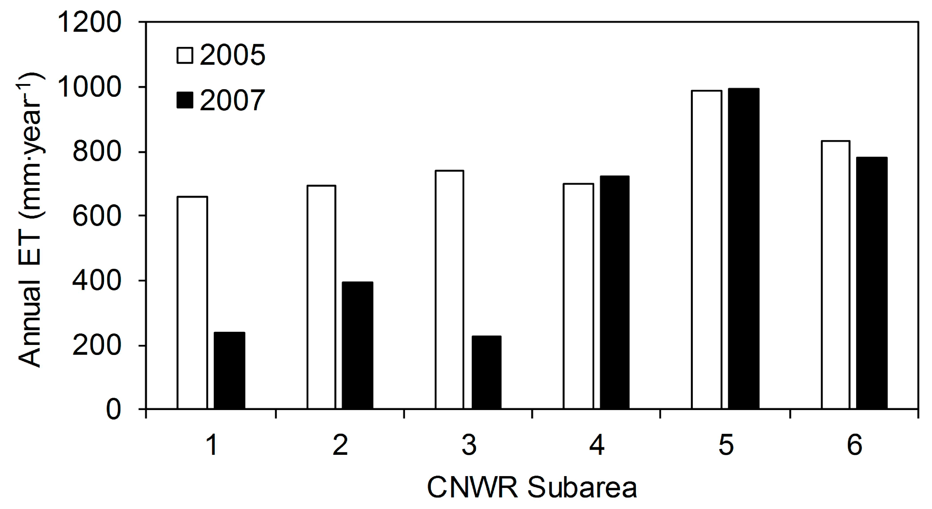
The massive wildfire of 2006 in the CNWR had a significant impact on riparian water use. The 4-year average annual SSS-ET after the wildfire (2007–2010) was 528 mm∙year−1, 30% smaller than the average (797 mm∙year−1) for the 4-year period before the fire (2002–2005). The wildfire had a greater impact in the northern parts of the CNWR (subareas 1, 2, and 3) as shown in Figure 10. The largest ET reduction was observed in subarea 3, where the ET reduced from 738 mm∙year−1 in 2005 to 227 mm∙year−1 in 2007 (69% reduction). Similarly, the annual ET over subareas 1 and 2 was reduced by 64% and 43%, respectively. Subareas 4, 5, and 6 showed a small reduction (3%), no change, and a small increase (6%) in water use between 2005 and 2007, respectively (Figure 11). This indicates that ET reductions in the northern subareas can be mainly attributed to the wildfire and not water stress caused by declines in groundwater levels. The potential impact of variable atmospheric demand was also ruled out, since ETo was 1774 mm∙year−1 in 2007, only 6% larger compared to ETo in 2005 (1668 mm∙year−1). The average 4-year ETo before and after the wildfire was 1720 mm∙year−1 and 1740 mm∙year−1, respectively. The lower ET rates over the northern parts of the CNWR due to wildfire of 2006 were also reported by [13].
Another wildfire occurred in the southern part of the CNWR in August 2011. Ref. [70] used a groundwater-based method to investigate changes in riparian water use pre- and post-fire at three locations in southern CNWR, and found both increases and decreases in ET after the wildfire of 2011. They reported that, after the wildfire, riparian ET decreased by 59% and 31% at two of the locations and increased by 8% at the third location. The study found groundwater depth was an important factor for defining ET rates before wildfire, whereas it was not a limiting factor after the wildfire, and that frequent burns in the CNWR most likely reduce annual ET rates. A wildfire’s impact on riparian water use may vary depending on multiple factors [71], including water availability, canopy development after wildfire, and advection of energy along riparian zones. In the short-term, riparian water use could increase by the abundance of sprouting shoots [8]. In the long-term, however, changes in forest composition by shifts in tree-age structure may reduce the forest leaf area compared to a pre-fire condition, ultimately decreasing the ET rates [72].
4. Conclusions
The single-satellite-scene (SSS) approach was applied to estimate the annual riparian water use over parts of the Cibola National Wildlife Refuge (CNWR) using Landsat TM5 imagery. The performance of the SSS method was assessed through comparing its results with those of a previously validated remotely sensed energy balance model at two distributed scales. At the pixel-based scale (comparisons for 1571 samples), the mean residual error was less than 104 mm∙year−1 (18%). The area-wide comparison was similar, showing an error of less than 95 mm∙year−1 (15%). The errors reduced by more than a half to less than 58 mm∙year−1 (7%) after excluding the areas with no to low vegetation from the analysis. These errors are in agreement with the reported errors of similar remote sensing approaches. In addition, they are within the error ranges of other major components of water balance for riparian ecosystems. Moreover, the results were not sensitive to the single image selected for analysis as long as that image was acquired during the peak vegetation cover. Hence, the SSS method can be used effectively to map annual water use over heterogeneous riparian forests.
The method was then applied to estimate riparian ET over a 23-year period from 1988 to 2010. The average annual ET varied from 483 to 915 mm∙year−1 during the study period, with an average of 748 mm∙year−1. A comparison with two readily available, independent sources of water use information revealed significant differences. The ET from the MODIS product (MOD16) was on average 82% smaller than the result of the SSS method. On the other hand, the U.S. Bureau of Reclamation’s Lower Colorado River Accounting System estimates were almost double that of the ET from the SSS method. Considering the simplicity and accuracy of the SSS approach, it has great potential to be the method of choice in estimating riparian ET and making informed water management decisions, especially in arid/semi-arid regions.
Despite significant advantages, the SSS method has three main limitations that must be considered before any application. As this method relies on remotely sensed NDVI and meteorological information, it may not able to account for factors that are not accounted for by NDVI. For example, water stresses that limit the ET rates are not instantly reflected in NDVI [13,15]. The second limitation is that this method requires homeostasis conditions, and thus will not provide accurate estimates if disturbances with significant impact on water use (e.g., wildfires, floods, and disease outbreaks) occur during part of the study year. Finally, the SSS method cannot account for direct evaporation from shallow groundwater.
Acknowledgments
Funding for this project was provided by the Oklahoma Agricultural Experiment Station and Oklahoma Cooperative Extension Service.
Author Contributions
Saleh Taghvaeian had the initial idea. Saleh Taghvaeian and Leila Hassan-Esfahani conceived and designed the experiment. All authors contributed to processing the data and interpreting the results. Kul Khand and Saleh Taghvaeian wrote the manuscript, and Leila Hassan-Esfahani revised it.
Conflicts of Interest
The authors declare no conflict of interest.
References
- Owens, M.K.; Moore, G.W. Saltcedar water use: Realistic and unrealistic expectations. Rangel. Ecol. Manag. 2007, 60, 553–557. [Google Scholar] [CrossRef]
- Zavaleta, E. Valuing Ecosystem Services Lost to Tamarix Invasion in the United States; Island Press: Washington, DC, USA, 2000; pp. 261–300. [Google Scholar]
- Glenn, E.P.; Nagler, P.L. Comparative ecophysiology of Tamarix ramosissima and native trees in western U.S. riparian zones. J. Arid Environ. 2005, 61, 419–446. [Google Scholar] [CrossRef]
- Glenn, E.; Tanner, R.; Mendez, S.; Kehret, T.; Moore, D.; Garcia, J.; Valdes, C. Growth rates, salt tolerance and water use characteristics of native and invasive riparian plants from the delta of the Colorado River, Mexico. J. Arid Environ. 1998, 40, 281–294. [Google Scholar] [CrossRef]
- Vandersande, M.W.; Glenn, E.P.; Walworth, J.L. Tolerance of five riparian plants from the lower Colorado River to salinity drought and inundation. J. Arid Environ. 2001, 49, 147–159. [Google Scholar] [CrossRef]
- Cleverly, J.R.; Smith, S.D.; Sala, A.; Devitt, D.A. Invasive capacity of Tamarix ramosissima in a Mojave Desert floodplain: The role of drought. Oecologia 1997, 111, 12–18. [Google Scholar] [CrossRef] [PubMed]
- Stromberg, J.C. Functional equivalency of saltcedar (Tamarix chinensis) and fremont cottonwood (Populus fremonth) along a free-flowing river. Wetlands 1998, 18, 675–686. [Google Scholar] [CrossRef]
- Busch, D.E.; Smith, S.D. Effects of fire on water and salinity relations of riparian woody taxa. Oecologia 1993, 94, 186–194. [Google Scholar] [CrossRef] [PubMed]
- Bailey, J.K.; Schweitzer, J.A.; Whitham, T.G. Salt cedar negatively affects biodiversity of aquatic macroinvertebrates. Wetlands 2001, 21, 442–447. [Google Scholar] [CrossRef]
- Harms, R.S.; Hiebert, R.D. Vegetation response following invasive tamarisk (Tamarix spp.) removal and implications for riparian restoration. Restor. Ecol. 2006, 14, 461–472. [Google Scholar] [CrossRef]
- Di Tomaso, J.M. Impact, biology, and ecology of saltcedar (Tamarix spp.) in the southwestern United States. Weed Technol. 1998, 12, 326–336. [Google Scholar]
- Murray, R.S.; Nagler, P.L.; Morino, K.; Glenn, E.P. An empirical algorithm for estimating agricultural and riparian evapotranspiration using MODIS Enhanced Vegetation Index and ground measurements of ET. II. Application to the Lower Colorado River, U.S. Remote Sens. 2009, 1, 1125–1138. [Google Scholar] [CrossRef]
- Nagler, P.L.; Morino, K.; Didan, K.; Erker, J.; Osterberg, J.; Hultine, K.R.; Glenn, E.P. Wide-area estimates of saltcedar (Tamarix spp.) evapotranspiration on the lower Colorado River measured by heat balance and remote sensing methods. Ecohydrology 2009, 2, 18–33. [Google Scholar] [CrossRef]
- Taghvaeian, S.; Neale, C.M.; Osterberg, J.; Sritharan, S.I.; Watts, D.R. Water use and stream-aquifer-phreatophyte interaction along a Tamarisk-dominated segment of the Lower Colorado River. In Remote Sensing of the Terrestrial Water Cycle; John & Sons, Inc.: Hoboken, NJ, USA, 2014; pp. 95–113. [Google Scholar]
- Nagler, P.L.; Scott, R.L.; Westenburg, C.; Cleverly, J.R.; Glenn, E.P.; Huete, A.R. Evapotranspiration on western U.S. rivers estimated using the Enhanced Vegetation Index from MODIS and data from eddy covariance and Bowen ratio flux towers. Remote Sens. Environ. 2005, 97, 337–351. [Google Scholar] [CrossRef]
- Scott, R.L.; Cable, W.L.; Huxman, T.E.; Nagler, P.L.; Hernandez, M.; Goodrich, D.C. Multiyear riparian evapotranspiration and groundwater use for a semiarid watershed. J. Arid Environ. 2008, 72, 1232–1246. [Google Scholar] [CrossRef]
- Gowda, P.H.; Chavez, J.L.; Colaizzi, P.D.; Evett, S.R.; Howell, T.A.; Tolk, J.A. ET mapping for agricultural water management: Present status and challenges. Irrig. Sci. 2008, 26, 223–237. [Google Scholar] [CrossRef]
- Morton, C.G.; Huntington, J.L.; Pohll, G.M.; Allen, R.G.; McGwire, K.C.; Bassett, S.D. Assessing calibration uncertainty and automation for estimating evapotranspiration from agricultural areas using METRIC. JAWRA J. Am. Water Resour. Assoc. 2013, 49, 549–562. [Google Scholar] [CrossRef]
- Irmak, A.; Allen, R.G.; Kjaersgaard, J.; Huntington, J.; Kamble, B.; Trezza, R.; Ratcliffe, I. Operational remote sensing of ET and challenges. In Evapotranspiration-Remote Sensing and Modeling; InTech: Reijaka, Croatia, 2012; pp. 467–492. [Google Scholar]
- Kalma, J.D.; McVicar, T.R.; McCabe, M.F. Estimating land surface evaporation: A review of methods using remotely sensed surface temperature data. Surv. Geophys. 2008, 29, 421–469. [Google Scholar] [CrossRef]
- Glenn, E.P.; Huete, A.R.; Nagler, P.L.; Hirschboeck, K.K.; Brown, P. Integrating remote sensing and ground methods to estimate evapotranspiration. Crit. Rev. Plant Sci. 2007, 26, 139–168. [Google Scholar] [CrossRef]
- Gonzalez-Dugo, M.P.; Neale, C.M.U.; Mateos, L.; Kustas, W.P.; Prueger, J.H.; Anderson, M.C.; Li, F. A comparison of operational remote sensing-based models for estimating crop evapotranspiration. Agric. For. Meteorol. 2009, 149, 1843–1853. [Google Scholar] [CrossRef]
- Bawazir, A.S.; Samani, Z.; Bleiweiss, M.; Skaggs, R.; Schmugge, T. Using ASTER satellite data to calculate riparian evapotranspiration in the Middle Rio Grande, New Mexico. Int. J. Remote Sens. 2009, 30, 5593–5603. [Google Scholar] [CrossRef]
- Kamble, B.; Irmak, A.; Martin, D.L.; Hubbard, K.G.; Ratcliffe, I.; Hergert, G.; Narumalani, S.; Oglesby, R.J. Satellite based energy balance approach to assess riparian water use. In Evapotranspiration—An Overview; InTech: Reijaka, Croatia, 2013; pp. 79–95. [Google Scholar]
- Liebert, R.; Huntington, J.; Morton, C.; Sueki, S.; Acharya, K. Reduced evapotranspiration from leaf beetle induced tamarisk defoliation in the Lower Virgin River using satellite-based energy balance. Ecohydrology 2016, 9, 179–193. [Google Scholar] [CrossRef]
- Qi, J.; Chehbouni, A.; Huete, A.R.; Kerr, Y.H.; Sorooshian, S. A modified soil adjusted vegetation index. Remote Sens. Environ. 1994, 48, 119–126. [Google Scholar] [CrossRef]
- Nichols, W.D. Regional Ground-Water Evapotranspiration and Ground-Water Budgets, Great Basin, Nevada; United States Geological Survey Professional Paper 1628; U.S. Geological Survey: Great Basin, NV, USA, 2000.
- Huete, A.; Didan, K.; Miura, T.; Rodriguez, E.P.; Gao, X.; Ferreira, L.G. Overview of the radiometric and biophysical performance of the MODIS vegetation indices. Remote Sens. Environ. 2002, 83, 195–213. [Google Scholar] [CrossRef]
- Nagler, P.L.; Glenn, E.P.; Nguyen, U.; Scott, R.L.; Doody, T. Estimating riparian and agricultural actual evapotranspiration by reference evapotranspiration and MODIS enhanced vegetation index. Remote Sens. 2013, 5, 3849–3871. [Google Scholar] [CrossRef]
- Tillman, F.D.; Callegary, J.B.; Nagler, P.L.; Glenn, E.P. A simple method for estimating basin-scale groundwater discharge by vegetation in the basin and range province of Arizona using remote sensing information and geographic information systems. J. Arid Environ. 2012, 82, 44–52. [Google Scholar] [CrossRef]
- Nagler, P.L.; Cleverly, J.; Glenn, E.; Lampkin, D.; Huete, A.; Wan, Z. Predicting riparian evapotranspiration from MODIS vegetation indices and meteorological data. Remote Sens. Environ. 2005, 94, 17–30. [Google Scholar] [CrossRef]
- Nagler, P.L.; Morino, K.; Murray, R.S.; Osterberg, J.; Glenn, E.P. An empirical algorithm for estimating agricultural and riparian evapotranspiration using MODIS enhanced vegetation index and ground measurements of ET. I. Description of method. Remote Sens. 2009, 1, 1273–1297. [Google Scholar] [CrossRef]
- Brouwer, C.; Heibloem, M. Irrigation Water Management Training Manual No. 3; FAO: Rome, Italy, 1986. [Google Scholar]
- Allen, R.G.; Clemmens, A.J.; Burt, C.M.; Solomon, K.; O’Halloran, T. Prediction accuracy for projectwide evapotranspiration using crop coefficients and reference evapotranspiration. J. Irrig. Drain. Eng. 2005, 131, 24–36. [Google Scholar] [CrossRef]
- Groeneveld, D.P.; Baugh, W.M.; Sanderson, J.S.; Cooper, D.J. Annual groundwater evapotranspiration mapped from single satellite scenes. J. Hydrol. 2007, 344, 146–156. [Google Scholar] [CrossRef]
- Groeneveld, D.P.; Baugh, W.M. Correcting satellite data to detect vegetation signal for eco-hydrologic analyses. J. Hydrol. 2007, 344, 135–145. [Google Scholar] [CrossRef]
- Beamer, J.P.; Huntington, J.L.; Morton, C.G.; Pohll, G.M. Estimating annual groundwater evapotranspiration from phreatophytes in the great basin using landsat and flux tower measurements. JAWRA J. Am. Water Resour. Assoc. 2013, 49, 518–533. [Google Scholar] [CrossRef]
- Groeneveld, D.P. Remotely-sensed groundwater evapotranspiration from alkali scrub affected by declining water table. J. Hydrol. 2008, 358, 294–303. [Google Scholar] [CrossRef]
- Glenn, E.P.; Jarchow, C.J.; Waugh, W.J. Evapotranspiration dynamics and effects on groundwater recharge and discharge at an arid waste disposal site. J. Arid Environ. 2016, 133, 1–9. [Google Scholar] [CrossRef]
- Barz, D.; Watson, R.P.; Kanney, J.F.; Roberts, J.D.; Groeneveld, D.P. Cost/benefit considerations for recent saltcedar control, Middle Pecos River, New Mexico. Environ. Manag. 2009, 43, 282. [Google Scholar] [CrossRef] [PubMed]
- Mexicano, L.; Glenn, E.P.; Hinojosa-Huerta, O.; Garcia-Hernandez, J.; Flessa, K.; Hinojosa-Corona, A. Long-term sustainability of the hydrology and vegetation of Cienega de Santa Clara, an anthropogenic wetland created by disposal of agricultural drain water in the delta of the Colorado River, Mexico. Ecol. Eng. 2013, 59, 111–120. [Google Scholar] [CrossRef]
- Nagler, P.L.; Brown, T.; Hultine, K.R.; van Riper, C.; Bean, D.W.; Dennison, P.E.; Murray, R.S.; Glenn, E.P. Regional scale impacts of Tamarix leaf beetles (Diorhabda carinulata) on the water availability of western U.S. rivers as determined by multi-scale remote sensing methods. Remote Sens. Environ. 2012, 118, 227–240. [Google Scholar] [CrossRef]
- Jarchow, C.J.; Nagler, P.L.; Glenn, E.P. Greenup and evapotranspiration following the Minute 319 pulse flow to Mexico: An analysis using Landsat 8 Normalized Difference Vegetation Index (NDVI) data. Ecol. Eng. in press. [CrossRef]
- Huete, A.R.; Liu, H.Q. An error and sensitivity analysis of the atmospheric-and soil-correcting variants of the NDVI for the MODIS-EOS. IEEE Trans. Geosci. Remote Sens. 1994, 32, 897–905. [Google Scholar] [CrossRef]
- Liu, H.Q.; Huete, A. A feedback based modification of the NDVI to minimize canopy background and atmospheric noise. IEEE Trans. Geosci. Remote Sens. 1995, 33, 457–465. [Google Scholar]
- Masek, J.G.; Vermote, E.F.; Saleous, N.; Wolfe, R.; Hall, F.G.; Huemmrich, F.; Gao, F.; Kutler, J.; Lim, T.K. LEDAPS Landsat Calibration, Reflectance, Atmospheric Correction Preprocessing Code; Model Product; Oak Ridge National Laboratory Distributed Active Archive Center: Oak Ridge, TN, USA, 2012. [CrossRef]
- Bastiaanssen, W.G.M.; Menenti, M.; Feddes, R.A.; Holtslag, A.A.M. A remote sensing surface energy balance algorithm for land (SEBAL). 1. Formulation. J. Hydrol. 1998, 212, 198–212. [Google Scholar] [CrossRef]
- Bastiaanssen, W.G.M.; Noordman, E.J.M.; Pelgrum, H.; Davids, G.; Thoreson, B.P.; Allen, R.G. SEBAL model with remotely sensed data to improve water-resources management under actual field conditions. J. Irrig. Drain. Eng. 2005, 131, 85–93. [Google Scholar] [CrossRef]
- Allen, R.G.; Tasumi, M.; Trezza, R. Satellite-based energy balance for mapping evapotranspiration with internalized calibration (METRIC)-Model. J. Irrig. Drain. Eng. 2007, 133, 380–394. [Google Scholar] [CrossRef]
- White, W.N. A Method of Estimating Ground-Water Supplies Based on Discharge by Plants and Evaporation from Soil: Results of Investigations in Escalante Valley, Utah; U.S. Government Printing Office: Washington, DC, USA, 1932; pp. 1–106.
- Environmental and Water Resources Institute of the American Society of Civil Engineers (ASCE-EWRI). The ASCE Standardized Reference Evapotranspiration Equation; Report of the ASCE-EWRI Task Committee on Standardization of Reference Evapotranspiration; ASCE: Reston, VA, USA, 2005. [Google Scholar]
- Mu, Q.; Heinsch, F.A.; Zhao, M.; Running, S.W. Development of a global evapotranspiration algorithm based on MODIS and global meteorology data. Remote Sens. Environ. 2007, 111, 519–536. [Google Scholar] [CrossRef]
- Mu, Q.; Zhao, M.; Running, S.W. Improvements to a MODIS global terrestrial evapotranspiration algorithm. Remote Sens. Environ. 2011, 115, 1781–1800. [Google Scholar] [CrossRef]
- Monteith, J. Evaporation and environment. Symp. Soc. Exp. Biol. 1965, 19, 205–234. [Google Scholar] [PubMed]
- United States Bureau of Reclamation. Lower Colorado River Accounting System. Evapotranspiration and Evaporation Calculations, Calendar Year 2005; United States Bureau of Reclamation: Boulder, NV, USA, 2007.
- United States Bureau of Reclamation. Lower Colorado River Accounting System. Evapotranspiration and Evaporation Calculations, Calendar Year 2010; United States Bureau of Reclamation: Boulder, NV, USA, 2014.
- Allen, R.G.; Pereira, L.S.; Howell, T.A.; Jensen, M.E. Evapotranspiration information reporting: I. Factors governing measurement accuracy. Agric. Water Manag. 2011, 98, 899–920. [Google Scholar] [CrossRef]
- Smith, J.L.; Laczniak, R.J.; Moreo, M.T.; Welborn, T.L. Mapping Evapotranspiration Units in the Basin and Range Carbonate-Rock Aquifer System, White Pine County, Nevada, and Adjacent Areas in Nevada and Utah; United States Geological Survey Scientific Investigations Report 2007-5087; U.S. Geological Survey: Reston, VA, USA, 2007.
- Allander, K.K.; Smith, J.L.; Johnson, M.J. Evapotranspiration from the Lower Walker River Basin, West-Central Nevada, Water Years 2005–07; United States Geological Survey Scientific Investigations Report 2009-5079; U.S. Geological Survey: Reston, VA, USA, 2009.
- Nagler, P.L.; Pearlstein, S.; Glenn, E.P.; Brown, T.B.; Bateman, H.L.; Bean, D.W.; Hultine, K.R. Rapid dispersal of saltcedar (Tamarix spp.) biocontrol beetles (Diorhabda carinulata) on a desert river detected by phenocams, MODIS imagery and ground observations. Remote Sens. Environ. 2014, 140, 206–219. [Google Scholar]
- Los Angeles Department of Water and Power (LADWP). Urban Water Management Plan; Arcadis U.S., Inc.: Los Angeles, CA, USA, 2015. [Google Scholar]
- Nagler, P.L.; Glenn, E.P.; Didan, K.; Osterberg, J.; Jordan, F.; Cunningham, J. Wide-Area Estimates of Stand Structure and Water Use of Tamarix spp. on the Lower Colorado River: Implications for Restoration and Water Management Projects. Restor. Ecol. 2008, 16, 136–145. [Google Scholar] [CrossRef]
- Friedl, M.A.; McIver, D.K.; Hodges, J.C.; Zhang, X.Y.; Muchoney, D.; Strahler, A.H.; Woodcock, C.E.; Gopal, S.; Schneider, A.; Baccini, A.; et al. Global land cover mapping from MODIS: Algorithms and early results. Remote Sens. Environ. 2002, 83, 287–302. [Google Scholar] [CrossRef]
- Friedl, M.A.; Sulla-Menashe, D.; Tan, B.; Schneider, A.; Ramankutty, N.; Sibley, A.; Huang, X. MODIS Collection 5 global land cover: Algorithm refinements and characterization of new datasets. Remote Sens. Environ. 2010, 114, 168–182. [Google Scholar] [CrossRef]
- Velpuri, N.M.; Senay, G.B.; Singh, R.K.; Bohms, S.; Verdin, J.P. A comprehensive evaluation of two MODIS evapotranspiration products over the conterminous United States: Using point and gridded FLUXNET and water balance ET. Remote Sens. Environ. 2013, 139, 35–49. [Google Scholar] [CrossRef]
- Ruhoff, A.L.; Paz, A.R.; Aragao, L.E.O.C.; Mu, Q.; Malhi, Y.; Collischonn, W.; Rocha, H.R.; Running, S.W. Assessment of the MODIS global evapotranspiration algorithm using eddy covariance measurements and hydrological modelling in the Rio Grande basin. Hydrol. Sci. J. 2013, 58, 1658–1676. [Google Scholar] [CrossRef]
- Biggs, T.W.; Marshall, M.; Messina, A. Mapping daily and seasonal evapotranspiration from irrigated crops using global climate grids and satellite imagery: Automation and methods comparison. Water Resour. Res. 2016, 52, 7311–7326. [Google Scholar] [CrossRef]
- Jensen, M.E. Vegetative and Open Water Coefficients for the Lower Colorado River Accounting System (Addendum to the 1998 Report); United States Bureau of Reclamation; Boulder Canyon Operations Office: Boulder City, NV, USA, 2003.
- Westenberg, C.; Harper, D.; DeMeo, G. Evapotranspiration by Phreatophytes Along the Lower Colorado River at Havasu National Wildlife Refuge, Arizona; United States Geological Survey Scientific Investigations Report, 2006-5043; U.S. Geological Survey: Henderson, NV, USA, 2006.
- Lewis, C.S. Evapotranspiration Estimation: A Study of Methods in the Western United States. Ph.D. Thesis, Civil Engineering-Utah State University, Logan, UT, USA, 2016. [Google Scholar]
- Devitt, D.A.; Sala, A.; Smith, S.D.; Cleverly, J.; Shaulis, L.K.; Hammett, R. Bowen ratio estimates of evapotranspiration for Tamarix ramosissima stands on the Virgin River in southern Nevada. Water Resour. Res. 1998, 34, 2407–2414. [Google Scholar] [CrossRef]
- Stromberg, J.C.; Rychener, T.J. Effects of fire on riparian forests along a free-flowing dryland river. Wetlands 2010, 30, 75–86. [Google Scholar] [CrossRef]
Figure 1.
Location of the study area in the Lower Colorado River Basin (left). The six subareas in the right panel indicate parts of the Cibola National Wildlife Refuge (CNWR) included in this study.
Figure 1.
Location of the study area in the Lower Colorado River Basin (left). The six subareas in the right panel indicate parts of the Cibola National Wildlife Refuge (CNWR) included in this study.

Figure 2.
Average Normalized Difference Vegetation Index (NDVI) of the study area for all cloud-free Landsat scenes in 2008. DOY, day of year.
Figure 2.
Average Normalized Difference Vegetation Index (NDVI) of the study area for all cloud-free Landsat scenes in 2008. DOY, day of year.

Figure 3.
Cumulative NDVI frequency distribution for DOYs 195 (a); 227 (b); and 259 (c).

Figure 4.
Comparison of annual single-satellite-scene evapotranspiration (SSS-ET) and remotely sensed energy balance evapotranspiration (RSEB-ET) for randomly selected samples within the CNWR.
Figure 4.
Comparison of annual single-satellite-scene evapotranspiration (SSS-ET) and remotely sensed energy balance evapotranspiration (RSEB-ET) for randomly selected samples within the CNWR.
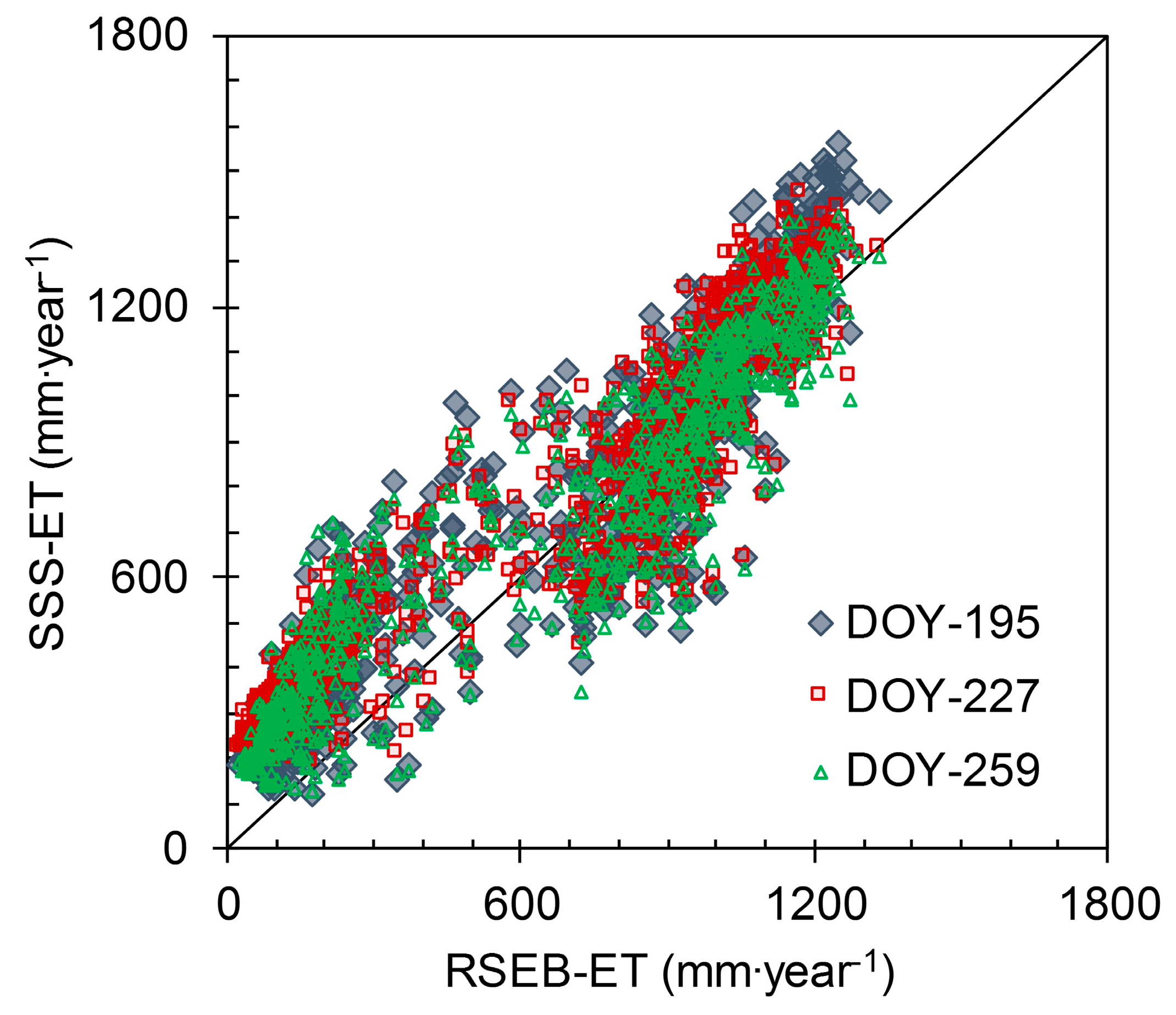
Figure 5.
(a–c) Comparison of annual SSS-ET and RSEB-ET for six subareas within the CNWR.

Figure 6.
Evapotranspiration (ET) differences (SSS–RSEB) versus NDVI for the three DOYs in 2008. Each point represents a subarea within the CNWR.
Figure 6.
Evapotranspiration (ET) differences (SSS–RSEB) versus NDVI for the three DOYs in 2008. Each point represents a subarea within the CNWR.

Figure 7.
Annual ET based on SSS, RSEB, and MOD16 for the year 2008.

Figure 8.
Annual ET from the CNWR obtained by the SSS method from 1988 to 2010.

Figure 9.
Comparison of annual ET over the California (CA) (solid) and Arizona (AZ) (dotted) regions of the CNWR. SSS-ET was not estimated for 2006 due to wildfire.
Figure 9.
Comparison of annual ET over the California (CA) (solid) and Arizona (AZ) (dotted) regions of the CNWR. SSS-ET was not estimated for 2006 due to wildfire.

Figure 10.
Landsat false color composite, NDVI, and annual ET before (top) and after (bottom) the wildfire of 2006.
Figure 10.
Landsat false color composite, NDVI, and annual ET before (top) and after (bottom) the wildfire of 2006.

Figure 11.
Annual SSS-ET for each CNWR subarea before and after the wildfire of 2006.


Table 1.
Summary of pixel-based and area-wide comparison of SSS-ET and RSEB-ET.
| Scale | DOY | SSS-ET (mm∙year−1) | RSEB-ET (mm∙year−1) | R2 | Residual Error (mm∙year−1) | Percent Error |
|---|---|---|---|---|---|---|
| Pixel-based | 195 | 693 | 589 | 0.86 | 104 | 17.7 |
| 227 | 692 | 589 | 0.87 | 103 | 17.5 | |
| 259 | 673 | 589 | 0.86 | 84 | 14.3 | |
| Area-wide | 195 | 732 | 637 | 0.97 | 95 | 14.9 |
| 227 | 727 | 637 | 0.96 | 90 | 14.1 | |
| 259 | 708 | 637 | 0.98 | 71 | 11.1 |
R2 = coefficient of determination.
Table 2.
Day of year (DOY) of selected Landsat images, their respective NDVIo and NDVIs, reference ET (ETo), precipitation, and estimated annual SSS-ET for 23 years of study.
Table 2.
Day of year (DOY) of selected Landsat images, their respective NDVIo and NDVIs, reference ET (ETo), precipitation, and estimated annual SSS-ET for 23 years of study.
| Year | DOY | NDVIo | NDVIs | ETo (mm∙year−1) | Precipitation (mm∙year−1) | SSS-ET (mm∙year−1) |
|---|---|---|---|---|---|---|
| 1988 | 220 | 0.08 | 1.00 | 1836 | 129 | 762 |
| 1989 | 238 | 0.07 | 0.92 | 1752 | 39 | 762 |
| 1990 | 241 | 0.06 | 0.94 | 1855 | 53 | 854 |
| 1991 | 244 | 0.07 | 0.88 | 1746 | 78 | 793 |
| 1992 | 215 | 0.08 | 0.83 | 1790 | 161 | 769 |
| 1993 | 217 | 0.09 | 1.00 | 1960 | 126 | 783 |
| 1994 | 236 | 0.08 | 0.89 | 2015 | 40 | 915 |
| 1995 | 223 | 0.09 | 0.88 | 1866 | 144 | 826 |
| 1996 | 226 | 0.08 | 0.95 | 1868 | 53 | 898 |
| 1997 | 212 | 0.08 | 0.93 | 1732 | 80 | 787 |
| 1998 | 215 | 0.09 | 0.96 | 1738 | 89 | 762 |
| 1999 | 218 | 0.08 | 1.00 | 1793 | 55 | 816 |
| 2000 | 221 | 0.07 | 0.87 | 1748 | 6 | 750 |
| 2001 | 223 | 0.07 | 0.87 | 1754 | 80 | 851 |
| 2002 | 226 | 0.08 | 0.87 | 1805 | 1 | 746 |
| 2003 | 229 | 0.07 | 0.92 | 1709 | 177 | 849 |
| 2004 | 248 | 0.08 | 1.00 | 1696 | 80 | 677 |
| 2005 | 218 | 0.10 | 0.90 | 1668 | 72 | 754 |
| 2006 | 237 | 0.07 | 0.91 | 1768 | 10 | NA |
| 2007 | 224 | 0.08 | 0.91 | 1774 | 10 | 508 |
| 2008 | 227 | 0.05 | 0.84 | 1815 | 1 | 598 |
| 2009 | 229 | 0.09 | 0.88 | 1728 | 19 | 524 |
| 2010 | 232 | 0.10 | 0.91 | 1644 | 19 | 483 |
NA = Not applicable due to wildfire.
© 2017 by the authors. Licensee MDPI, Basel, Switzerland. This article is an open access article distributed under the terms and conditions of the Creative Commons Attribution (CC BY) license (http://creativecommons.org/licenses/by/4.0/).
Share and Cite
MDPI and ACS Style
Khand, K.; Taghvaeian, S.; Hassan-Esfahani, L. Mapping Annual Riparian Water Use Based on the Single-Satellite-Scene Approach. Remote Sens. 2017, 9, 832. https://doi.org/10.3390/rs9080832
AMA Style
Khand K, Taghvaeian S, Hassan-Esfahani L. Mapping Annual Riparian Water Use Based on the Single-Satellite-Scene Approach. Remote Sensing. 2017; 9(8):832. https://doi.org/10.3390/rs9080832
Chicago/Turabian StyleKhand, Kul, Saleh Taghvaeian, and Leila Hassan-Esfahani. 2017. "Mapping Annual Riparian Water Use Based on the Single-Satellite-Scene Approach" Remote Sensing 9, no. 8: 832. https://doi.org/10.3390/rs9080832
Note that from the first issue of 2016, this journal uses article numbers instead of page numbers. See further details here.