Challenges in Methane Column Retrievals from AVIRIS-NG Imagery over Spectrally Cluttered Surfaces: A Sensitivity Analysis


1
College of Marine Science, University of South Florida, 140 7th Ave. South, St. Petersburg, FL 33701, USA
2
Bubbleology Research International, 1642 Elm Ave, Solvang, CA 93463, USA
*
Author to whom correspondence should be addressed.
Remote Sens. 2017, 9(8), 835; https://doi.org/10.3390/rs9080835
Submission received: 12 May 2017
/
Revised: 2 August 2017
/
Accepted: 8 August 2017
/
Published: 12 August 2017
(This article belongs to the Special Issue Remote Sensing of Greenhouse Gases)
Abstract
:A comparison between efforts to detect methane anomalies by a simple band ratio approach from the Airborne Visual Infrared Imaging Spectrometer-Classic (AVIRIS-C) data for the Kern Front oil field, Central California, and the Coal Oil Point marine hydrocarbon seep field, offshore southern California, was conducted. The detection succeeded for the marine source and failed for the terrestrial source, despite these sources being of comparable strength. Scene differences were investigated in higher spectral and spatial resolution collected by the AVIRIS-C successor instrument, AVIRIS Next Generation (AVIRIS-NG), by a sensitivity study. Sensitivity to factors including water vapor, aerosol, planetary boundary layer (PBL) structure, illumination and viewing angle, and surface albedo clutter were explored. The study used the residual radiance method, with sensitivity derived from MODTRAN (MODerate resolution atmospheric correction TRANsmission) simulations of column methane (XCH4). Simulations used the spectral specifications and geometries of AVIRIS-NG and were based on a uniform or an in situ vertical CH4 profile, which was measured concurrent with the AVIRIS-NG data. Small but significant sensitivity was found for PBL structure and water vapor; however, highly non-linear, extremely strong sensitivity was found for surface albedo error. For example, a 10% decrease in the surface albedo corresponded to a 300% XCH4 increase over background XCH4 to compensate for the total signal, less so for stronger plumes. This strong non-linear sensitivity resulted from the high percentage of surface-reflected radiance in the airborne at-sensor total radiance. Coarse spectral resolution and feedback from interferents like water vapor underlay this sensitivity. Imaging spectrometry like AVIRIS and the Hyperspectral InfraRed Imager (HyspIRI) candidate satellite mission, have the advantages of contextual spatial information and greater at-sensor total radiance. However, they also face challenges due to their relatively broad spectral resolution compared to trace gas specific orbital sensors, e.g., the Greenhouse gases Observing SATellite (GOSAT), which is especially applicable to trace gas retrievals over scenes with high spectral albedo variability. Results of the sensitivity analysis are applicable for the residual radiance method and CH4 profiles used in the analysis, but they illustrate potential significant challenges in CH4 retrievals using other approaches.
1. Introduction
1.1. Methane
The potent greenhouse gas (GHG), methane (CH4) is the second most important anthropogenic gas affecting the global radiative balance after carbon dioxide (CO2). CH4 is 34 times stronger as a heat-trapping gas than CO2 on a 100-year timescale (86 times on a 20-year timescale) [1]. About 60–70% of global CH4 emissions arise from anthropogenic sources including rice agriculture, fossil fuel industrial (FFI) production, waste handling, and domestic ruminants [2]. Important natural CH4 sources include wetlands, termites, and geological seepage [3].
Given that CH4’s atmospheric residence time is only ~8.5 years [4]—i.e., far shorter than the century timescale of CO2, there are advantages to addressing global warming through CH4 emission regulations compared to CO2 [5]. Since pre-industrial times, CH4 concentrations have risen, with the increase rate slowing and then almost stopping between 1999 and 2006, but growth has resumed since 2007 [6,7]. A number of mechanisms have been proposed to underlie these trends [6,8,9]; however, high uncertainty in emissions complicates interpretations. For example, a recent study suggested that FFI emissions are one and a half times greater than previous inventory estimates [10], while those of husbandry also appear to be underestimated significantly [11]. Given that accurate inventories are key to effective mitigation strategies, there is a critical need for new approaches to assess emissions to improve inventories.
The National Oceanic and Atmospheric Administration (NOAA) tower network provides in situ, highly accurate CH4 measurements. Still, it cannot improve inventories at the regional (or national in many cases), local, or facility scale due to the scarcity of the observing stations [12]. In contrast, satellites provide global coverage and repeat measurements at high data density allowing effective monitoring of CH4 concentrations at regional to local scales, if the sensor has sufficient resolution [13]. Necessarily, retrieval algorithm validation for current and future satellite missions is required to enable satellite data to improve inventories. Airborne remote sensing data can play a critical validation role.
1.2. Methane Remote Sensing
Only satellite remote sensing provides the global coverage to address emissions on the global scale needed to address factors underlying greenhouse warming. The first global map of tropospheric CH4 was provided by the SCanning Imaging Absorption spectroMeter for Atmospheric CHartographY (SCIAMACHY) instrument launched in 2002 [14], which operated through 2012 at a 30 × 60 km resolution. More recently, the currently operational Greenhouse gases Observing SATellite (GOSAT) operated by Japan Aerospace Exploration Agency (JAXA), provides global column CH4 (XCH4, see definition in Table 1) by means of proxy and physics-based algorithms [15,16,17]. GOSAT observes at 10 × 10 km spatial resolution and is a sampling mission. The Thermal And Near infrared Sensor for carbon Observation (TANSO)—Fourier Transform Spectrometer (FTS) onboard GOSAT uses spectral absorption features near 1.6 μm for CH4 retrieval with 0.2 cm−1 spectral intervals and 0.27 cm−1 spectral resolution. The coarse spatial resolution of these satellite instruments (and sampling nature of GOSAT) challenges facility-level monitoring sources with their data. The Sentinel 5 precursor mission, TROPOspheric Monitoring Instrument (TROPOMI), is scheduled to launch in 2017 with a 7 km spatial resolution, followed by the Sentinel 5 mission in 2021, to provide daily global mapping coverage of XCH4 and XCO2 [18].
Existing airborne systems can remotely sense CH4 at finer than satellite scales, using either non-imaging or imaging spectrometers. Airborne non-imaging sensors have higher sensitivity to CH4, an example being the Methane Airborne MAPper (MAMAP) sensor [19], whereas imaging sensors have lower sensitivity, but include contextual information, examples being the instrument Mako [20] and HyTes [21] that use the thermal infrared (TIR), and Airborne Visual InfraRed Imaging Spectrometer-Classic (AVIRIS-C) [22] and AVIRIS-Next generation (AVIRIS-NG) [23] spectrometers that use the short-wave infrared (SWIR). AVIRIS-C and AVIRIS-NG specifications are provided in Section 2.1.
A number of approaches have been developed to retrieve XCH4 from airborne and satellite data. These approaches include qualitative ones such as band-ratio approach [24], cluster-tuned matched filter (CTMF) approach [25], and quantitative ones such as the Weighting Function Modified (WFM) Differential Optical Absorption Spectroscopy (DOAS) algorithm [14], and the Iteratively Maximum a Posteriori DOAS (IMAP-DOAS) algorithm [26].
1.3. Study Motivation
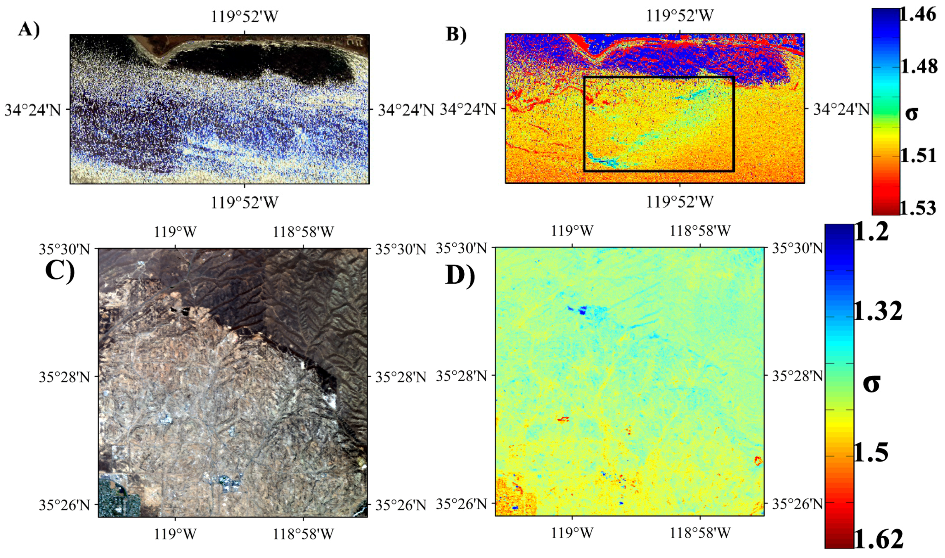
Real-world applications of radiative transfer models to atmospheric simulations almost always incorporate imperfect information given that in situ profile data and surface spectral data generally are unavailable. Imperfect information propagates into biases in the trace gas retrievals. This study is developed out of a scoping study that compared XCH4 for two scenes of comparable emission strength, one marine and one terrestrial—i.e., different radiative transfer characteristics and surface spectral complexity. The scoping study used a simple band-ratio method [24], which is computationally fast and can screen large datasets to identify spatial subsets for more sophisticated analysis. Specifically, the scoping study analyzed AVIRIS-C acquired 19 June 2008 for the Coal Oil Point (COP) marine seep field and 6 June 2013 for the Kern Front oil field (terrestrial) (Figure 1). This is a producing oil field and is located near Bakersfield, California, in the central San Joaquin Valley, California. Emissions have been estimated at ~1.0–1.5 ×10⁵ m3 day−1 (25 Gg year−1) [27] for the COP seep field. Emissions for the Kern Front oil field were estimated at ~60 Gg year−1 in September 2014, decreasing exponentially to ~30 Gg year−1 by late 2015 [28].
The scoping study revealed a dramatic performance difference for XCH4 retrievals (Figure 1). Strong CH4 plumes were easily detected for the marine source, but were highly challenged for the terrestrial source. The main purpose of the present study was to better understand these differences through a series of sensitivity studies testing different factors that could influence the XCH4 retrievals including albedo, water vapor, observational geometry, aerosol, and surface spectral heterogeneity. Findings are evaluated with respect to implications for airborne and spaceborne remote sensing sensors. Sensitivity was studied through forward modeling using MODTRAN, the spectral specifications and geometries of AVIRIS Next Generation (AVIRIS-NG), and the residual radiance, also termed the residual radiance method. The residual radiance method has been used for successful trace gas detection of the offshore emissions from the COP seep field [29]. For simplicity, the modeling is for a uniform surface, despite the fact that in reality many surfaces can exhibit complicated effects in their Bi-directional Reflectance Distribution Functions (BRDF). The study focused on understanding factors leading to the band ratio’s poor performance for the Kern oil fields and how they also impact a more sophisticated approach, the residual radiance method. These sensitivity study results are directly applicable only to the residual radiance method for XCH4 retrievals. Still, the findings have implications for other retrieval methods due to common radiative transfer challenges, such as spectral clutter, particularly for moderate spectral resolution instruments.
2. Materials and Methods
2.1. Imaging Spectrometers
AVIRIS-C is a whiskbroom sensor that collects radiance from 380 to 2500 nm in 224 channels with a ~10 nm bandwidth and 1 milliradian [30]. AVIRIS-NG is the successor instrument to AVIRIS-C and is a pushbroom sensor that collects spectra in 432 bands at a sampling interval of 5 nm and a Full Width at Half Maximum (FWHM) varying from 5.6 to 6.0 nm. AVIRIS-NG has improved geo-location and signal to noise ratio (SNR) over AVIRIS-C (SNR > 1000 @ 600 nm and > 800 @ 2200 nm, at an input reflectance level of 25%) [31]. A Gaussian function was employed to describe the slit function. The cross-track swaths of the AVIRIS-C and AVIRIS-NG are 892 and 795 pixels, respectively, with an angular swath width of 30°.
Dennison et al. [32] reported that the NEδL of AVIRIS-NG is one third that of AVIRIS-C, which Green & Pavri [33] estimated at 0.001 mW cm−2 μm−1 sr−1. For this study, the NEδL is taken as 0.00035 mW cm−2 μm−1 sr−1 for AVIRIS-NG. Important geometric parameters include solar zenith angle (θs), sensor viewing zenith angle (θv) and relative sun-sensor azimuth angle (φ). Jet Propulsion Laboratory provided geo-referenced radiance data and observation geometries.
2.2. Study Area
The sensitivity study used the observation geometry, surface albedo from AVIRIS-NG imagery acquired for the Kern River oil field (Figure 2), located immediately north of Bakersfield, CA. CH4 leakage plumes have been documented by remote sensing for this active oil field [20], as well as by in situ observations [28].
Supporting this study are data collected during the CO2 and Methane EXperiment (COMEX) [34]. COMEX combined in situ airborne and surface data, with airborne imaging and non-imaging spectroscopy to explore synergies between these remote sensing approaches for GHG emission estimation. COMEX investigated southern California CH4 sources including husbandry, landfills, natural geology, and FFI refining and production, the latter being the strongest among the COMEX foci.
This study leveraged the availability of simultaneous in situ profile and AVIRIS-NG data, to understand the impact of erroneous vertical CH4 profile on XCH4. Two profile cases were simulated, in situ profile and a uniform profile (see Figure 3B). The two profiles have the same column-averaged CH4 within a boundary layer of 2.0 km. In situ data were collected in a data curtain (Figure 3A and Figure A1) by the CIRPAS Twin Otter airplane (www.cirpas.org) above the Kern Front oil field [19].
The CIRPAS acquisition was concurrent (to a few hours) with the AVIRIS-NG acquisition. In situ CH4 concentrations were measured by an onboard Cavity Ringdown Spectrometer (Picarro Inc., Mountainview, CA, USA). Data in the survey plane were segregated as in the plume or outside, averaged at each altitude level, and then interpolated linearly between levels. Data identified the Planetary Boundary Layer (PBL) at ~1.2 km (Figure 3B and Figure A2). Additional details on the measurement and derivation of the in situ profile are provided in Appendix A.1. The “uniform profile” presumed a well-mixed atmosphere (vertically uniform) to 2.0 km altitude. For all two cases, the profile above 2.0 km was that of a typical mid-latitude summer atmosphere.
2.3. Radiative Transfer Simulations—Residual Radiance Method
MODTRAN has a long history of being applied to trace gas retrievals, e.g., Roberts et al. [29] and Thorpe et al. [25]. In this study, we use MODTRAN5.3.2 to model Lt for the AVIRIS-NG sensor viewing and illumination geometries and bandwidth (5 nm). Gaussian slit functions were used in the simulations. Two plume simulation scenarios were considered, a uniform profile and an in situ profile (Section 2.2). The atmosphere simulated was a typical mid-latitude summer atmosphere. Thus, the default mid-latitude CH4 profile was used for above 2.0 km. Visibility was derived from the atmospheric correction of AVIRIS-NG using the Fast Line-of-sight Atmospheric Analysis of Spectral Hypercubes (FLAASH) module in Environment for Visualizing Images (ENVI) for an urban aerosol. Water vapor column was derived from the water absorption feature that overlaps the 1135 nm band. AVIRIS-NG data provided the land cover spectra and observation geometries for the sensitivity analysis.
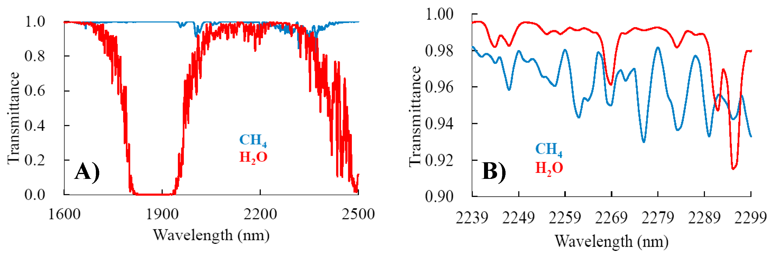
The residual radiance method for CH4 retrieval is detailed in Roberts et al. [29], and summarized briefly below. In this study, the method was used in forward modeling to evaluate whether two modeled total radiance spectra (using different input parameters) agreed with each other. First, the at-sensor radiance (Lt) was simulated for a surface albedo (ρs) of 0.1 and the aerosol and water vapor derived using the method described above. The true ρs was approximated by comparing the simulated Lt with the observed Lt for 2139 nm, under the assumption that Lt increases linearly with ρs. The 2139 nm band was used to estimate ρs because it is the band closest to the CH4 spectral absorption feature (2239–2299 nm) that also is free of CH4 absorption (Figure 4A). ρs in the wavelength range of 2239–2299 nm was assumed to be equal to ρs for 2139 nm—a spectral flatness assumption. Spectral flatness may not be a valid assumption for some land surface types, introducing biases in XCH4. A new radiative transfer simulation was carried out using the newly calculated ρs and a background XCH4, from which a new set of Lt were derived. The average residual radiance (Δ) was calculated by averaging the subtraction of the AVIRIS-NG observed Lt from the simulated Lt (denoted by Ltsim) for bands from 2239 to 2299 nm, where CH4 had stronger absorption than water vapor (Figure 4B).
Note, a large ∆ corresponds to high CH4 absorption—i.e., high XCH4. It should be noted that the residual radiance method for XCH4 retrieval was presented in this paper by forward simulations for calculating residual radiance that was used to derive the sensitivity.
2.4. Sensitivity Studies
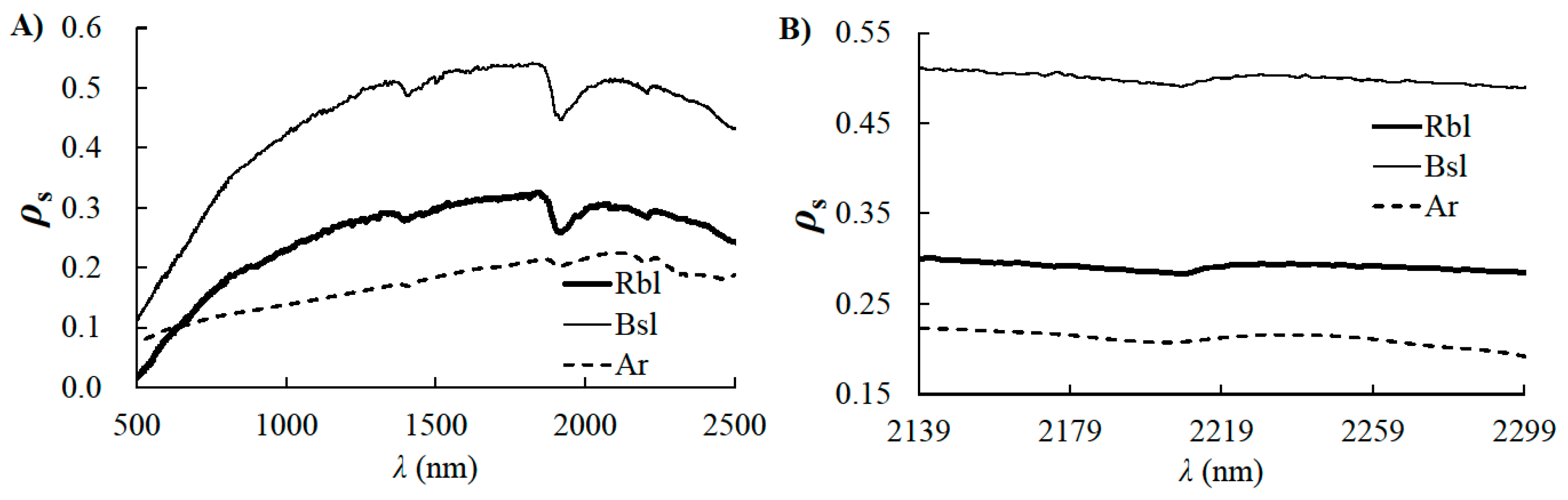
The sensitivity of XCH4 to surface albedo was based on the hypothesis that errors in surface albedo propagate through the MODTRAN calculations manifesting as an error in XCH4 that produces the same measured Lt. Because of the underlying key importance of surface albedo, sensitivity studies were referenced to the spectra of three common scene elements in the Kern Front oil field imagery: Asphalt road, Brown sandy loam, and Reddish-brown sandy loam, noted as Ar, Bsl, and Rbl, respectively (Figure 5). These three scene elements span a range of occurrence probabilities in the AVIRIS-NG imagery, with Rbl being dominant (Figure A3 in Appendix A.2). The three surface types differ in terms of both magnitude and shape of the spectral reflectance, which deviate slightly from a spectrally flat behavior (see Figure 5B).
Within the CH4 absorption feature, increases (decreases) in XCH4 will decrease (increase) Lt. Thus, inaccurate ρs biases XCH4. The retrieved XCH4 sensitivity to ρs was evaluated through MODTRAN simulations for a XCH4 “base-scenario”, denoted XCH4_b, with respect to relative error in ρs, denoted α, which spanned from −50% to 50%. Lt(λi) for different values of α was derived for the 13 AVIRIS-NG bands from 2239 to 2299 nm, denoted Lt(α, λi). Using the original ρs, the increase (for α < 0) or decrease (for α > 0) in XCH4 relative to XCH4_b was determined by error minimization, which minimized the average residual radiance () until convergence, defined as < NEδLa, where NEδLa is the average over the N bands spanning the feature, i.e.,
where N is 13, and i is the band number. For convenience, we denoted XCH4_err for the residual-radiance minimized XCH4 for ρs with respect to α. Finally, we defined the sensitivity to α for the CH4 column, S(XCH4_b, α):
A negative (positive) α means underestimation (overestimation), which causes an overestimation (underestimation) of XCH4 and as a result S(XCH4_b, α) is positive (negative).
Taking a negative α as an example, the error minimization was carried out as follows. XCH4 is increased from XCH4_b by a specified interval (e.g., 0.01 ppm). For each increase, Lt was simulated and applied to Equation (2) to calculate Δ. The increase continues until in Equation (2) is smaller than NEδLa.
Using the same method for deriving the sensitivity to albedo as described above, sensitivities to water vapor and to spectral flatness were also investigated. The sensitivity to scene geometry (or aerosol, vertical profile) was derived by calculating S(XCH4_b, α) using the method described above for different geometries (or aerosols, vertical profiles) while other parameters were kept unchanged.
3. Results
3.1. Sensitivity Studies
The sensitivity study investigated the relative importance of the various differing factors between the scenes to understand the relative importance of the factors underlying the difference between the band ratio analysis of the Kern versus the COP scenes. Sensitivity studies are for the residual radiance method. Factors include surface albedo, vertical profile, scene geometry, spectra flatness, water vapor, and aerosols.
3.1.1. Sensitivity to Albedo Error
The simulations showed that XCH4 exhibited an extremely strong and non-linear sensitivity to ρs error (α), with the relative error in Lt(λ) (β) for the plume simulation exhibiting a significant but linear sensitivity—note how β(α) lies on the 1:1 line (Figure 6A). The albedo error sensitivity with respect to XCH4 was explored by varying the plume strength from k = 0 (background, XCH4_A) to k = 1 (in situ profile) to k = 10 (factor of 10 stronger plume than observed), i.e.,
XCH4 = XCH4_A + k × XCH4_P
Here, XCH4_P is the plume anomaly, such that XCH4_A + XCH4_P is the vertical plume profile. Simulations revealed a significant and non-linear XCH4 error resulted from the error in ρs for the observed plume (k = 1), a sensitivity that was close to invariant with land cover types (Figure 6B). This albedo error sensitivity in XCH4 was explored further for the dominant scene element, Rbl by varying the plume anomaly strength from k = 0 to k = 10 (Figure 6C). S(XCH4_b, α), is highly nonlinear (Figure 6C), albeit less so for stronger plumes (k > 1). For example, for α = −5% for pixel Rbl, S decreased from 144.3% to 18.5% for XCH4 increasing from background (k = 0) to a very strong plume (k = 10). XCH4 could not be retrieved for α higher than 5% for XCH4 plumes of k = 0, 0.1, 0.25. For the k = 10 plume, XCH4 could not be retrieved for α higher than 45%. This means no XCH4 could be found that would meet the convergence requirements of Equations (2) and (3).
3.1.2. Variation of Albedo Sensitivity with Vertical CH4 Profile
Comparison between the simulations showed that the measured profile, with a shallower PBL, reduced sensitivity (S(XCH4_b, α)) by 9–12% compared to a uniform profile (Figure 8). The sensitivity difference resulting from the difference in vertical CH4 distribution indicated that path dependency was a factor that should be considered in the CH4 retrieval. This showed that at a minimum, the importance of using appropriate PBL thicknesses for retrievals in different regions, using realistic profiles, if available, is naturally the best option.
3.1.3. Variation of Albedo Sensitivity with Scene Geometry
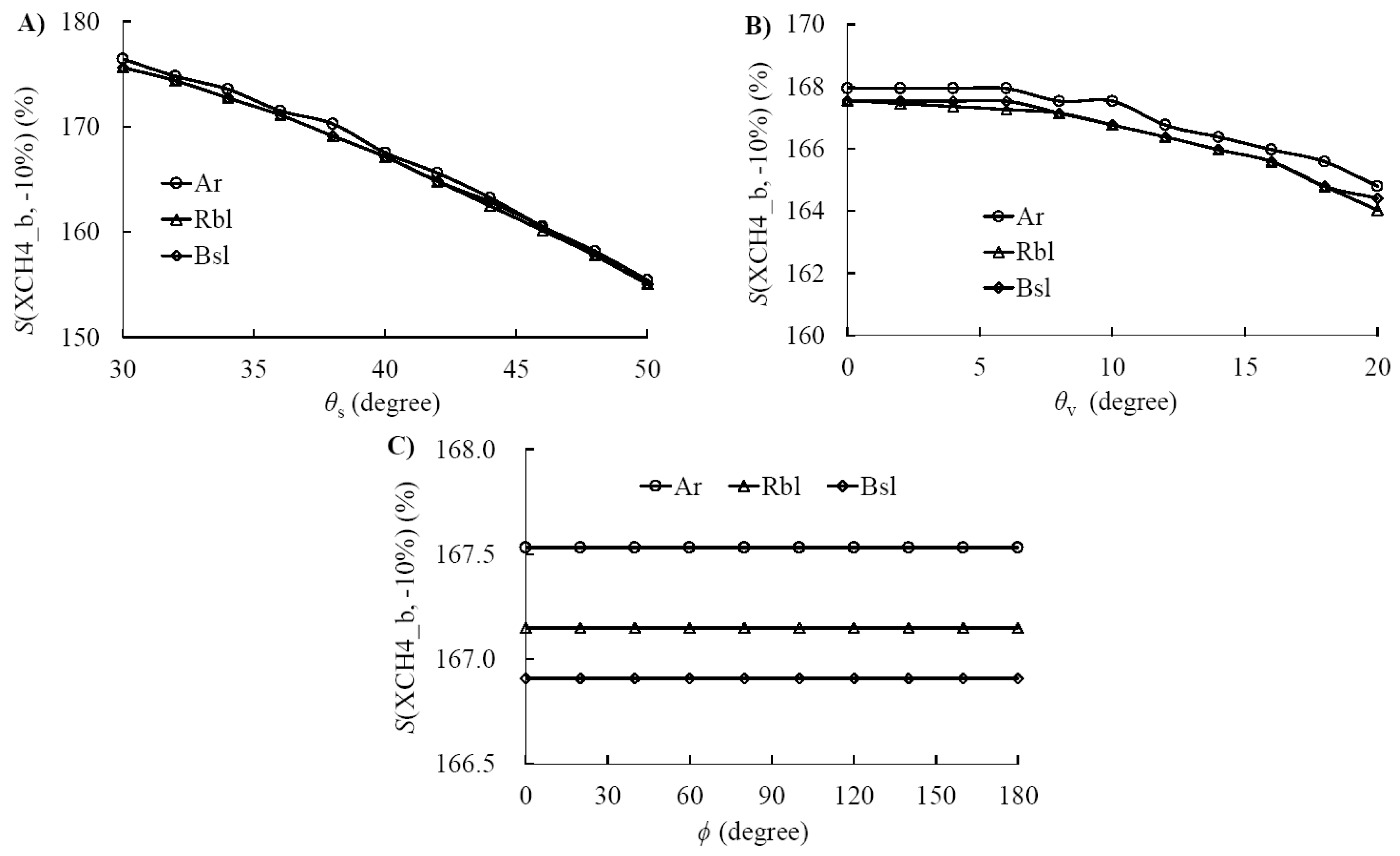
Scene geometry sensitivity was investigated by simulations for the k = 1 plume, with solar zenith angle (θs) varied from 30° to 50°, sensor viewing zenith angle (θv) varied from 0° to 20°, and relative sun-sensor azimuth angle (φ) varied from 0° to 180°. With respect to observation geometry, S(XCH4_b, α) exhibits the strongest angular sensitivity to θs (Figure 9A), with little difference between scene elements. S(XCH4_b, α) is related inversely to increases in θs and θv but is constant with φ due to the simulations’ Lambertian surface characterization (Figure 9). The relatively strong angular sensitivity to θs and θv is probably due to that the relative contribution from the surface scattering versus from atmospheric scattering decreases with increasing θs or θv.
3.1.4. Variation of Albedo Sensitivity with Aerosol Type and Visibility
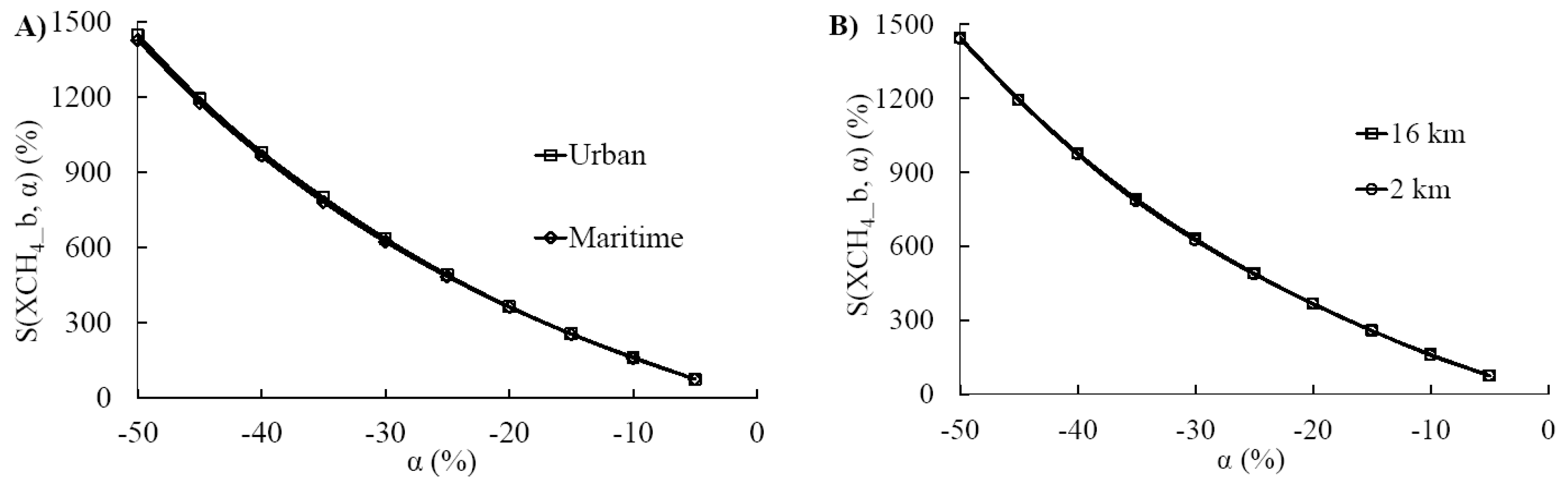
Given the similarity in S(XCH4_b, α) between surface spectral composition for the parameters studied, aerosol sensitivity was studied only for Rbl pixel and showed no significant difference in S(XCH4_b, α) between the two highly distinct aerosol types considered, urban and marine (Figure 10)—163% vs. 160% for urban compared to the marine atmosphere. Thus, the discrepancy between clearly detected plumes in the marine environment (Figure 1B) and no detectable plumes for the urban terrestrial environment (Figure 1D) was not due to the significant differences between marine and terrestrial aerosol. The overestimation changed from 160.8% for a 16-km visibility to 157.7% for 2-km visibility.
3.1.5. Sensitivity to Spectral Flatness
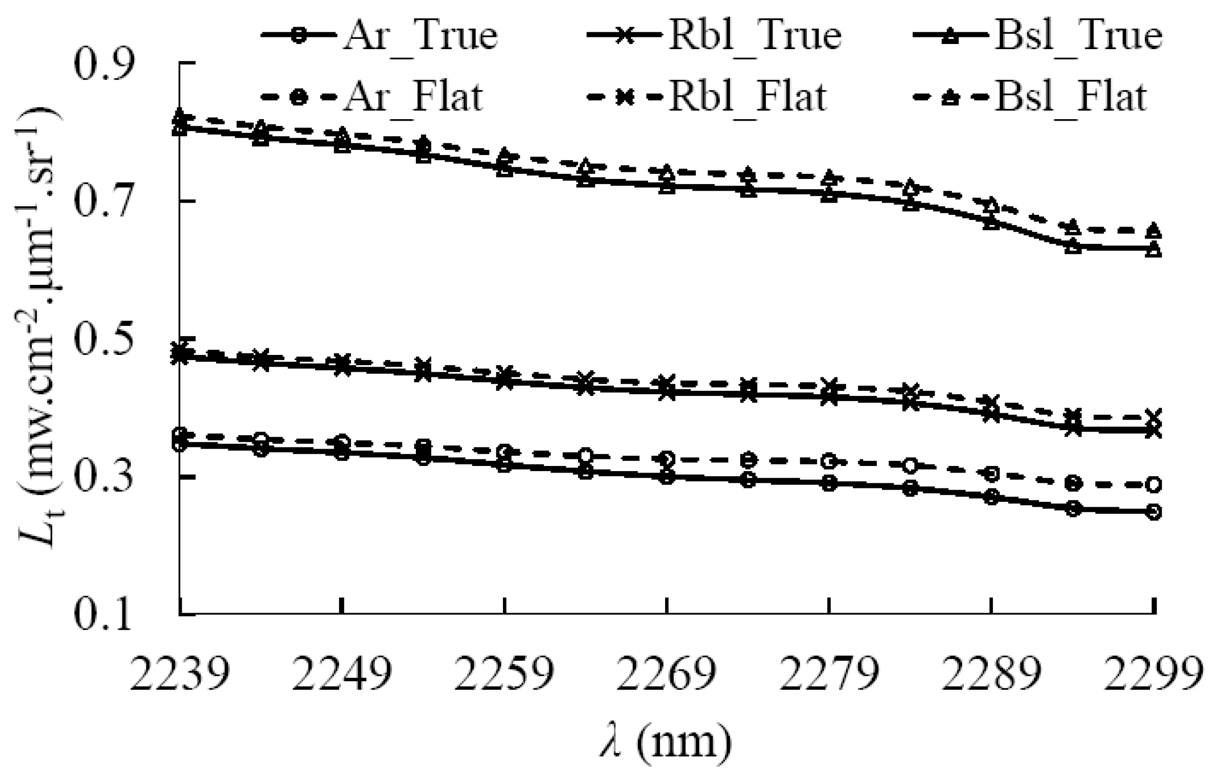
The residual radiance method [29] has an underlying important spectral flatness assumption. In reality, ρs(λ) varies with λ for a water surface in the spectral range of the CH4 absorption feature, decreasing from 2139 to 2299 nm. Simulations showed that the flat spectra assumption led to an overestimation of the calculated Lt compared with the true albedo spectra (Figure 11). The overestimation in Lt increased with, longer λ and resulted in a non-negligible underestimation of XCH4. Table 2 further quantified this underestimation, which decreased with brighter surface pixels. Furthermore, this underestimation in Lt increased with a decrease in XCH4_b. In fact, for the background (k = 0), XCH4 could not be retrieved for the pixel Ar with XCH4_A for the constant surface albedo assumption based on albedo at 2139 nm (Table 2). The underestimation decreased to 30% for Ar and to 8.1% for Bsl as XCH4 increased from background to the k = 1 plume.
3.1.6. Sensitivity to Water Vapor
Water vapor was retrieved from Moderate Resolution Imaging Spectroradiometer (MODIS) data using a ratio of radiance in a band with water vapor absorption (905 or 940 nm) to that in a band free of the absorption (865 nm). The retrieved water vapor has been validated by in situ data, with a relative error estimated at ~7% [35]. In a study by Albert et al. [36], MODIS retrieved water vapor by means of a differential absorption technique was compared with the field measurements taken by microwave water radiometer. A relative deviation of 9.4% was derived from the comparison.
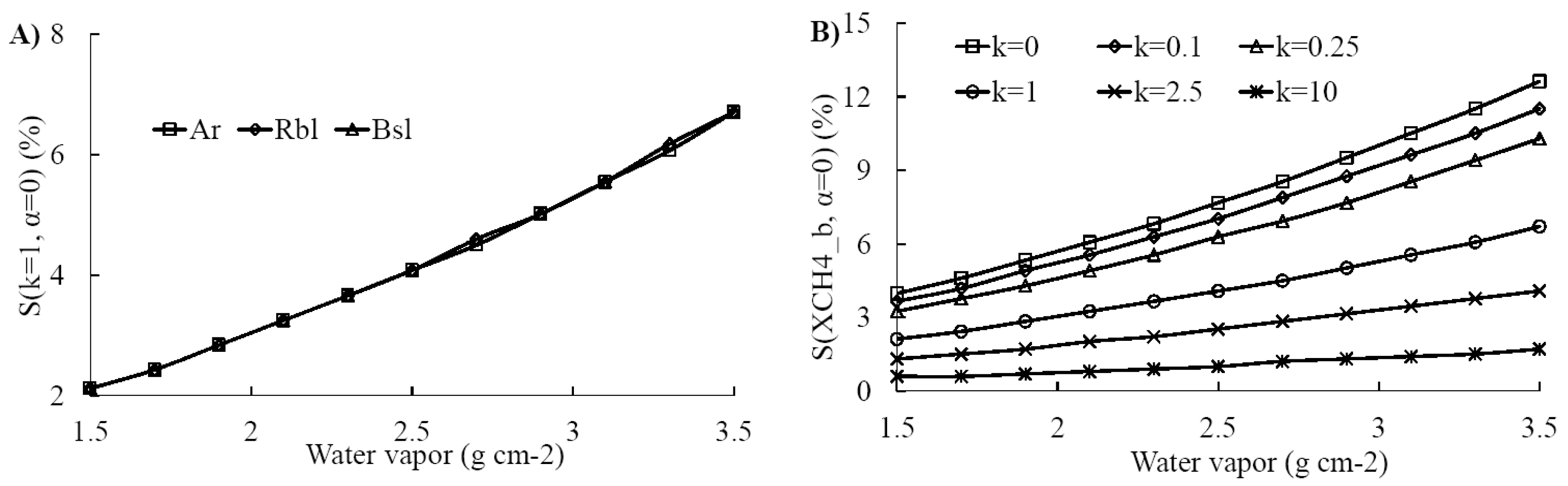
A sensitivity study based on a 9% uncertainty in AVIRIS-NG, water vapor retrievals (Figure 12) showed a detectable S(XCH4_b, α = 0) overestimation. Specifically, S(XCH4_b, α = 0) increased with the increase of water vapor while it decreased with increasing XCH4. Overall, S(XCH4_b, α = 0) varied little with the land cover types.
3.2. Space-Based Retrieval Sensitivity to Subpixel Spectral and CH4 Heterogeneity
To investigate the sensitivity of XCH4 to subpixel spectral heterogeneity, simulations were conducted for a simplified GOSAT pixel—a 10 × 10 km square (rather than round)—for 666 km altitude. The GOSAT pixel was divided into 160 × 160 subpixels with spatial resolution of 62.5 m, approximately the spatial resolution of the Hyperspectral Infrared Imager (HyspIRI) mission, which has a planned 10-nm spectral resolution [37]. For this simulation, the albedos of a 100 km2 subset of the AVIRIS-NG data, subset into 160 × 160 pixels, was derived from imagery acquired on 4 September 2014 (Figure 2, red box). Note, concurrent GOSAT data were unavailable for the Kern area on 4 September 2014.
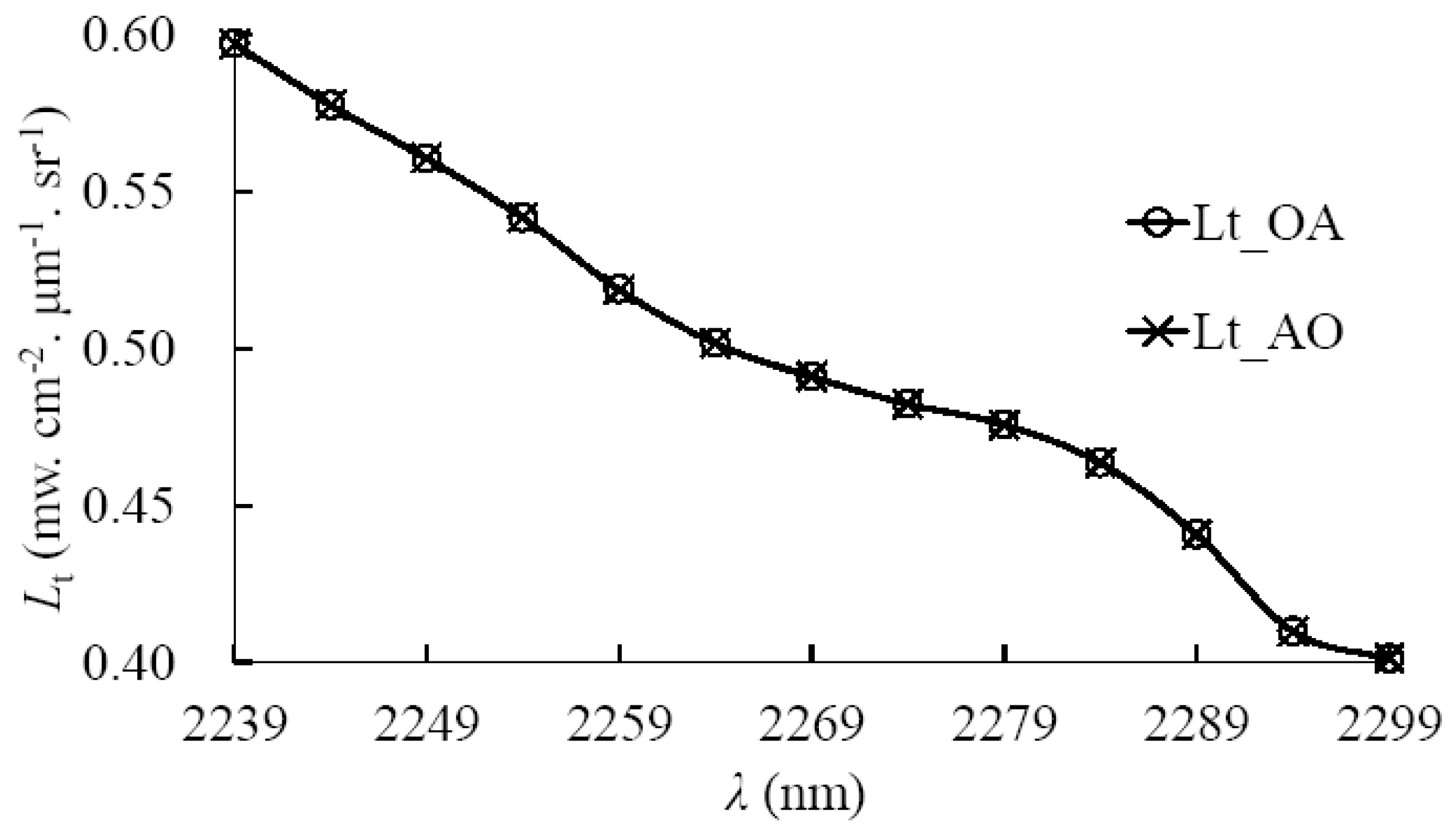
Lt for the GOSAT pixel was simulated for the in situ profile (i.e., k = 1, Figure 3) by two approaches. In the first case, denoted Lt_AO, Lt was simulated for each of the 160 × 160 pixels using each pixel’s ρs, and the orbital Lt then was averaged to produce the GOSAT pixel Lt. In the second case, denoted Lt_OA, the average ρs for the 160 × 160 pixels was calculated first, from which the GOSAT pixel Lt then was derived. The notation reflected whether spatial averaging occurred before or after extending AVIRIS-NG ρs to the orbital sensor, respectively. The calculated Lt_AO and Lt_OA across the spectral area of interest were essentially identical (Figure 13), demonstrating linearity for the response of Lt to ρs.
Although in some conditions, e.g., a well-mixed background PBL, GOSAT pixels were approximated reasonably well on the sub-pixel level as having homogeneous XCH4; for many GOSAT pixels, XCH4 was spatially heterogeneous. On the GOSAT size-scale, this heterogeneity was dominated by the overall plume dimensions; however, even on the vastly finer AVIRIS-NG size scale, strong heterogeneity exists due to plume structure, including puffiness [23].
The importance of spatial XCH4 heterogeneity was investigated by simulations over a pixel of the same size as GOSAT, which was divided into 160 × 160 subpixels with a spatial resolution of 62.5 m. The Lt and albedo for these subpixels were from the AVIRIS-NG imagery acquired on 4 September 2014 (Figure 2, red box). The mean Lt and XCH4 over the pixel are denoted by Lt_GOSAT and XCH4_GOSAT, respectively. Then, using the average albedo for all the subpixels, simulations were carried out by varying XCH4 to minimize the average residual radiance between the simulated Lt and Lt_GOSAT until it was smaller than the band-averaged NEδL (NEδLa). The error minimized XCH4 is denoted XCH4_M. It is important to note that XCH4_M was smaller than XCH4_GOSAT. Figure 14 shows the XCH4 underestimation (γ) with respect to percentage area coverage by the CH4 plume in a pixel of the same size as GOSAT (Pc). Note the pixel size is fixed while Pc is varied.
Variations in Pc change for the average XCH4. For example, a pixel with the mean XCH4 = 0.5 ppm, a 5% variation of Pc implies that 5% of the 160 × 160 subpixels were covered by a plume with XCH4 = 10 ppm. In this case, the forward simulation indicates that a XCH4 of 0.35 ppm can be observed over the pixel (γ is equal to 0.15 ppm). As Pc decreases, γ increases but γ also increases for increasing XCH4 plume strength, e.g., γ increases from 0.01 to 0.15 ppm when Pc decreases from 60% to 5% for an anomaly of 0.5 ppm. Thus, biases can become significant if the pixel percent coverage by a strong plume is small.
4. Discussion and Conclusions
4.1. Scoping Study
The scoping study identified a surprising difference in performance of the band ratio approach for similar strength sources from the COP marine seep field and for Kern Front oil field (Figure 1). The band ratio approach clearly detected plumes for the marine source, while plumes were not apparent for the terrestrial source. Key differences between these settings include water vapor, aerosol, and surface albedo heterogeneity—often termed spectral clutter.
Using a forward simulation and a residual radiance approach (as in the CH4 detection algorithm in Roberts et al. [29]), sensitivity of XCH4 to a variety of factors was investigated. The greatest sensitivity was from surface albedo (Figure 6, Figure A4 and Figure A5). A −5% error in surface albedo could cause a relative error up to 144.3% depending on the CH4 concentration. Such a strong sensitivity arises from the high percentage of the surface reflected radiance in the total radiance received by AVIRIS-NG. Even a small error in surface albedo requires a large XCH4 to compensate in the total radiance spectrum. Sensitivity to scene-differing factors other than surface albedo error, such as scene geometry, aerosols, and water vapor was small, although some were important in terms of accurate retrievals. For example, sensitivity to water vapor showed a 9% overestimation of water vapor (equivalent to 1.9 g cm−2) results in a 4.6% overestimation for background XCH4. Despite significant differences in aerosol between a marine atmosphere (COP) and a terrestrial atmosphere (Kern Front), aerosol was found to be of negligible importance to the different scene retrieval performances. As a result, the non-albedo sensitivity factors cannot explain the difference in retrieval performance between the scenes.
Surface albedo error also induces uncertainty in retrieved trace gas column in a second manner due to spectral non-flatness. Specifically, the assumption of spectral flatness in Roberts et al. [29] was investigated and found to introduce significant uncertainty in XCH4, up to over 100%, depending on the plume strength and the underlying pixel surface type. This spectral factor occurs in synergy with albedo error, and illustrates the importance of accurately retrieving the surface albedo spectra, within and across the CH4 absorption feature.
Above all, the non-linear sensitivity of XCH4 to the albedo error could explain most of the difference in the retrieval performance between two different scenes. It should also be noted from Noël et al. (2012) that the distortion of the slit function for an inhomogeneously illuminated slit could also be another reason for the difference in retrieval performance [38].
4.2. In Situ Versus Uniform Profile
The simplest profile is a well-mixed PBL—i.e., uniform with altitude; which was quite distinct from the real profile where concentration decreased rapidly with altitude in the upper PBL, with a sharp decrease above (Figure 3). In the simulations, the column was held the same for the two, to test sensitivity to albedo error, and found a 9–12% increase in albedo error sensitivity. In other words, the realistic profile improved retrieval performance against artifacts resulting from surface albedo error.
4.3. Interferents
Accurate surface albedo is critical to any retrieval method, and this study found it to be highly sensitive for the residual radiance retrieval approach. In part, this non-linearity arose from radiative interaction between water vapor and CH4 column, both of which depend on surface albedo. Finer spectral resolution would enable better deconvolution of these factors (AVIRIS-NG versus AVIRIS-C), decreasing the albedo error sensitivity. In the limit, extremely fine spectral resolution sensors, e.g., SCHIAMACHY, that resolve individual absorption lines, avoid most of the problems of assumed spectral flatness, which, while potentially significant over tens of nanometers, are minimal across a single line.
4.4. Retrieval Method and Future Work
This sensitivity study used the forward simulation and residual radiance; thus the results are directly applicable only to the residual radiance method for XCH4 retrieval. As noted above, surface albedo is critical to any retrieval method, particularly if the cluttered surface includes material with spectral features in the wavelengths of the trace gas. For example, carbonates have spectral features in the 2.4 µm CH4 feature. Thorpe et al. [22], found that the IMAP-DOAS approach, which succeeded at CH4 retrievals for AVIRIS imagery for the COP seep field, was challenged by retrievals for a terrestrial scene. Specifically, they noted that “disentangling surface spectral signatures from the methane absorption features is complicated”. Some approaches are likely to be less sensitive, such as the singular value decomposition hybrid IMAP-DOAS approach adopted by Thorpe et al. [22] to address complex terrestrial scenes. Higher spatial resolution may or may not reduce sub-pixel element heterogeneity, depending on how the end members are organized spatially. Albedo error uncertainty is largest if the spectral contrast in the absorption feature between end members is large; thus pixels at water/ice-land boundaries present very strong contrasts that will introduce relatively larger uncertainty. Specifically, the different pixel end members introduce positive and negative biases that are non-linear and thus do not cancel when combined to calculate XCH4 for the pixel. This would not be true if the biases were linear, in which case they would cancel when combined. One approach is to statistically model surface composition outside the plume, as an application for plume pixels. This approach is challenged by non-statistical surfaces such as river banks and urban areas where natural laws do not govern pixel end member component distributions.
These simulations were for a uniform surface; however, many surfaces exhibit complicated BRDF. The importance of realistic scene BRDF should be explored in further studies.
In any case, the fundamental importance of surface albedo to retrievals shows a need for investigating the sensitivity of different retrieval algorithms, to better understand the advantages and limitations of each approach, with respect to different applications. This is particularly important for broad spectral resolution instruments like AVIRIS-C, AVIRIS-NG, and the candidate HyspIRI orbital mission, as well as for spectrometers with finer spatial resolution.
Acknowledgments
We gratefully acknowledge the support of NASA Earth Sciences Division (Grant NNX12AQ16G). We also appreciate the contribution from CIRPAS, of the Naval Postgraduate School and NASA Ames Research Center, Richard Koyler, and Christopher Melton of Bubbleology Research International, for providing in situ profile data. Two anonymous reviewers provided extensive comments and suggestions to help improve this manuscript, whose effort is greatly appreciated.
Author Contributions
Ira Leifer designed the research experiment and contributed to the structure, writing, and editing of the manuscript. Chuanmin Hu contributed to editing of the manuscript. Minwei Zhang performed the data analysis, made figures, and wrote the manuscript.
Conflicts of Interest
The authors declare no conflict of interest.
Appendix A
Appendix A.1. In Situ Measurements
The Center for Interdisciplinary Remotely Piloted Aircraft Studies CIRPAS Twin Otter airplane collected airborne in situ greenhouse gas and meteorology data. The CIRPAS standard instrumentation suite includes temperature, 3D winds, humidity, and aerosol. More information on the CIRPAS instrumentation suite is found at www.cirpas.org [39]. Furthermore, in situ airborne measurements were made by a cavity-ringdown spectrometer, which sampled at 10 Hz and provided CH4 within 0.1 ppm (G-2301f, Picarro Inc., Santa Clara, CA, USA). The Picarro instrument used a direct current (DC)- powered external vacuum pump (N920, KNF Labs, Trenton, NJ, USA) connected to the main air sample inlet port by a 0.46 cm diameter and 3.28 m long PTFE tube. Lab calibrations were performed with gas standards before and after aircraft integration and used to assess instrument stability and develop corrections for drift.
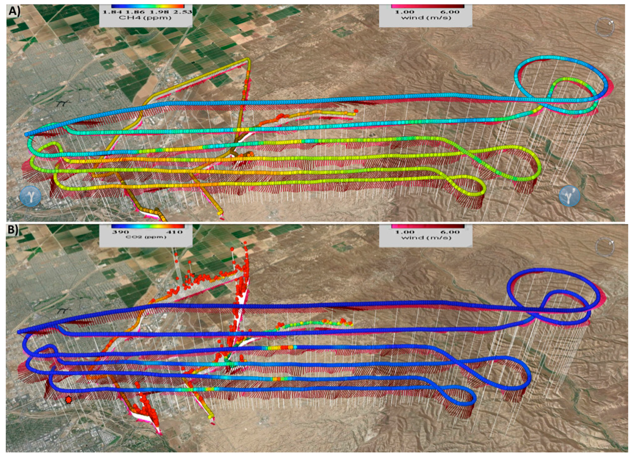
In situ CIRPAS data mapped multiple distinct, strong CH4 plumes, including several that penetrated above the PBL, as well as a clearly defined and also strong, broad-based plume (Figure A1A). CO2 plumes were far more localized (vertically and horizontal) than the CH4 plumes (Figure A1B).
Figure A1.
(A) Methane (CH4) and (B) carbon dioxide (CO2), and winds for 4 September 2014 from airborne in situ (CIRPAS) and surface mobile in situ (AMOG surveyor). Red star shows data curtain zero point (119.0411°W, 35.3972°N). Data keys on panels.
Figure A1.
(A) Methane (CH4) and (B) carbon dioxide (CO2), and winds for 4 September 2014 from airborne in situ (CIRPAS) and surface mobile in situ (AMOG surveyor). Red star shows data curtain zero point (119.0411°W, 35.3972°N). Data keys on panels.

The anomaly was determined relative to a background concentration (Figure A1), defined as the peak of a best-fit Gaussian function to the concentration probability histogram of each transect at each altitude in the data curtain.
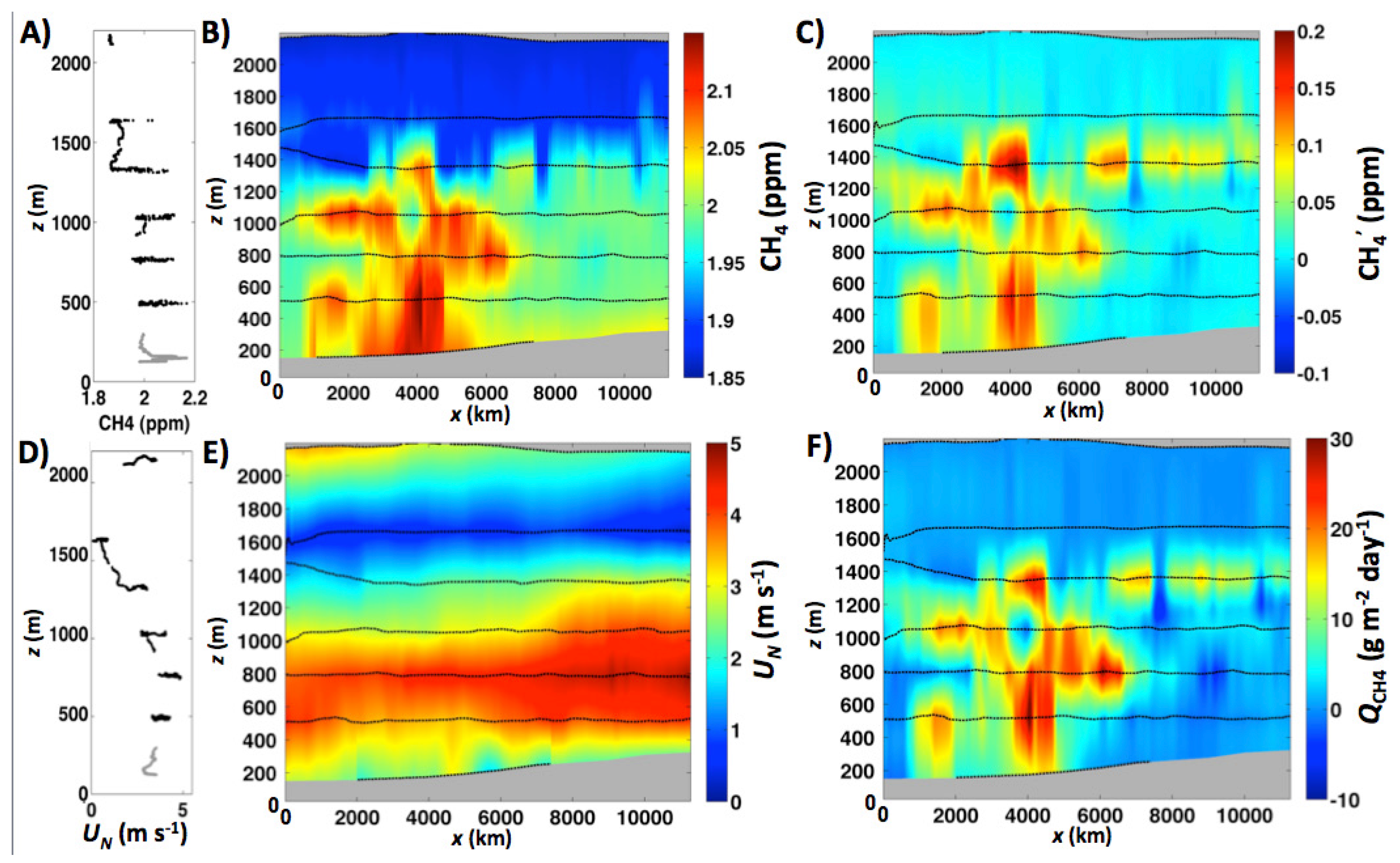
Winds were strongest slightly below the top of the PBL (Figure A2D), where a broad, thin CH4 plume was observed at ~800–1000 m altitude (Figure A2B). This would be consistent with rising buoyant plumes that were too weak to penetrate above the PBL. Several strong, lower altitude plumes were identified at 500 m altitude, which most likely originated in the near field to the curtain. Subtracting the background concentration field (Figure A2C) yielded the CH4 anomaly (CH4’) (Figure A2F).
Figure A2.
(A) Downwind methane (CH4) vertical profile with altitude (z) for Kern Front oil field transect (Figure A1) on 4 September 2014, and (B) Transect curtain, vertically-interpolated CH4(x, z), where x is easting distance relative to 119.0411°W, 35.3972°N. Dashed line shows data locations with gray for ground and above airborne data. Where surface data were unavailable, surface values were extrapolated from CAMOG/CCIRPAS(500 m) and (C) CH4 anomaly (CH4′(x,z)) based on background subtraction, (D) plane-normal wind profile (UN(z)), as in panel A, (E) transect curtain UN(x,z) and (F) transect curtain of CH4 flux (QCH4(x,z)). Data key on panels.

Appendix A.2. Scene Element Selection
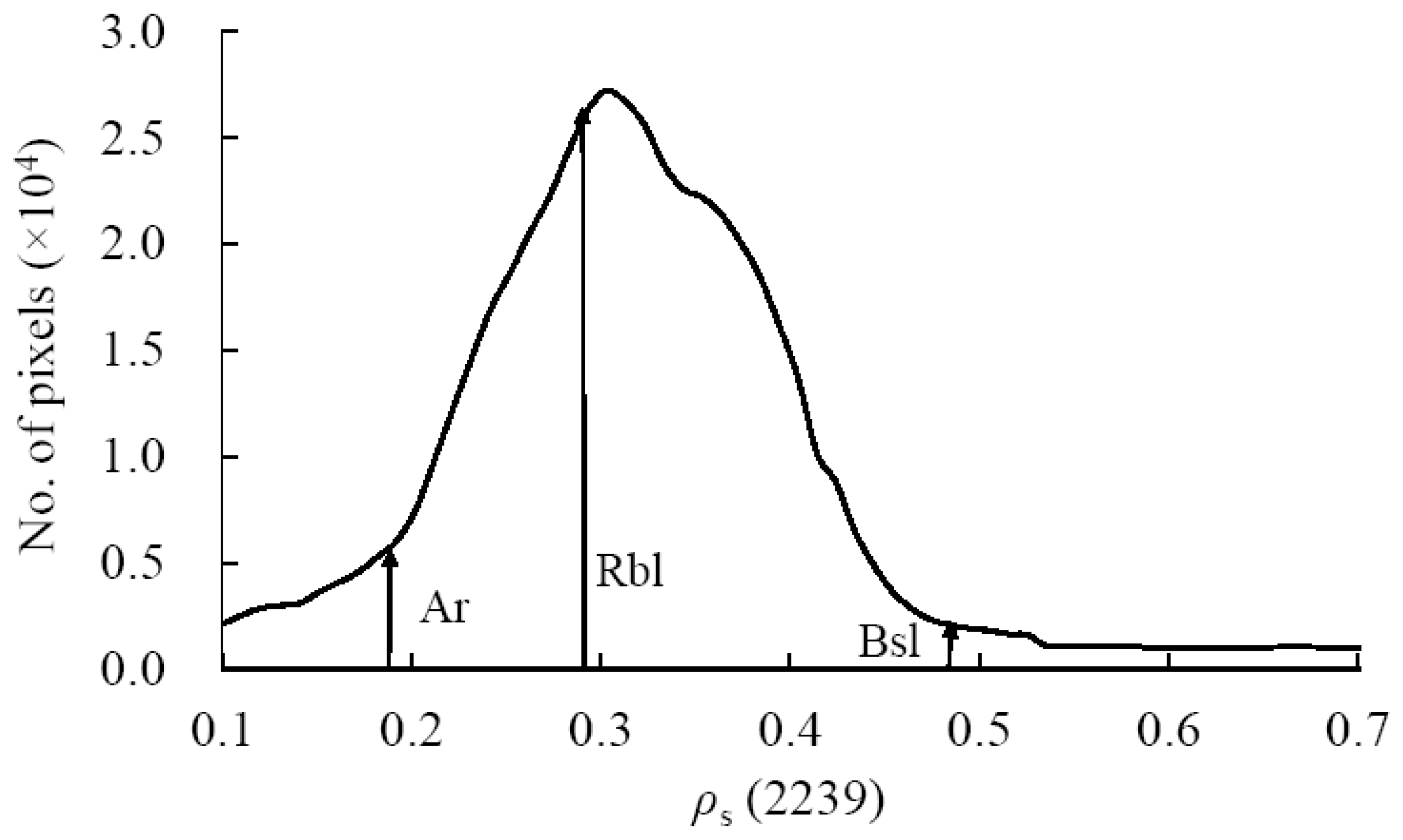
FLAASH was applied to the atmospheric correction of AVIRIS-NG data acquired on 4 September 2014, from which we derived surface albedo (ρs). Based on a histogram of occurrence probability, we selected three pixels with surface albedos spanning the dominant scene range albedo range at 2239 nm (CH4 absorption feature), specifically, 0.19, 0.29, and 0.48 (Figure A3).
Figure A3.
Scene occurrence histogram for surface albedo (ρs) for 2239 nm derived from FLAASH atmospheric correction of AVIRIS-NG data on 4 September 2014. ρs(2239) for the three pixels Asphalt road (Ar), Brown sandy loam (Bsl), and Reddish brown sandy loam (Rbl), identified on figure.
Figure A3.
Scene occurrence histogram for surface albedo (ρs) for 2239 nm derived from FLAASH atmospheric correction of AVIRIS-NG data on 4 September 2014. ρs(2239) for the three pixels Asphalt road (Ar), Brown sandy loam (Bsl), and Reddish brown sandy loam (Rbl), identified on figure.

Element pixel occurrence was calculated from a spectral similarity parameter between AVIRIS-NG retrieved ρs and albedo spectra in ENVI spectral library. The parameter combines Euclidean distance with correlation coefficient [40]. The albedo spectra with the smallest similarity parameter among those in the spectral library were used in the sensitivity simulation. The histogram confirmed that elements with these albedos, Asphalt road, Ar, Brown sandy loam, Bsl, and Reddish-brown sandy loam, Rbl, were in fact common scene elements, with Rbl dominant.
Appendix A.3. Requirement for ρs Accuracy in Terms of Accuracy of GOSAT Retrieved XCH4
GOSAT-measured XCH4 is biased low by 1.2 ± 1.1% compared with the measurements from ground-based high-resolution Fourier Transform Spectrometers in Total Carbon Column Observing Network (TCCON) [41]. The XCH4 retrieved by means of a proxy method and a physics method is compared with ground-based XCH4 measurements at 12 stations. The retrieval bias for the proxy method ranges from −0.321% to 0.421% with a standard deviation of 0.22%. The range is from −0.836% to −0.081% and the standard deviation is 0.24% for the physics method [17]. Through accurate O2A-band modeling, the bias decreases to −0.30% with a standard deviation of the bias about 0.26% [42]. Considering all these validations, 0.5% was selected as the relative error of GOSAT retrieved XCH4. Table A1 shows the requirement for the accuracy of surface albedo if the accuracy of AVIRIS-NG retrieved XCH4 reaches that of GOSAT measured XCH4.

Table A1.
Minimum requirement for the accuracy of ρs if the accuracy of AVIRIS-NG retrieved XCH4 reaches that for GOSAT measured XCH4.
Table A1.
Minimum requirement for the accuracy of ρs if the accuracy of AVIRIS-NG retrieved XCH4 reaches that for GOSAT measured XCH4.
| XCH4 | Relative Error (%) | ||
|---|---|---|---|
| Ar | Rbl | Bsl | |
| k = 0 | 0.065 | 0.064 | 0.065 |
| k = 0.1 | 0.073 | 0.076 | 0.077 |
| k = 1 | 0.11 | 0.11 | 0.12 |
| k = 10 | 0.27 | 0.27 | 0.26 |
Appendix A.4. Accuracy of Remotely Sensed ρs
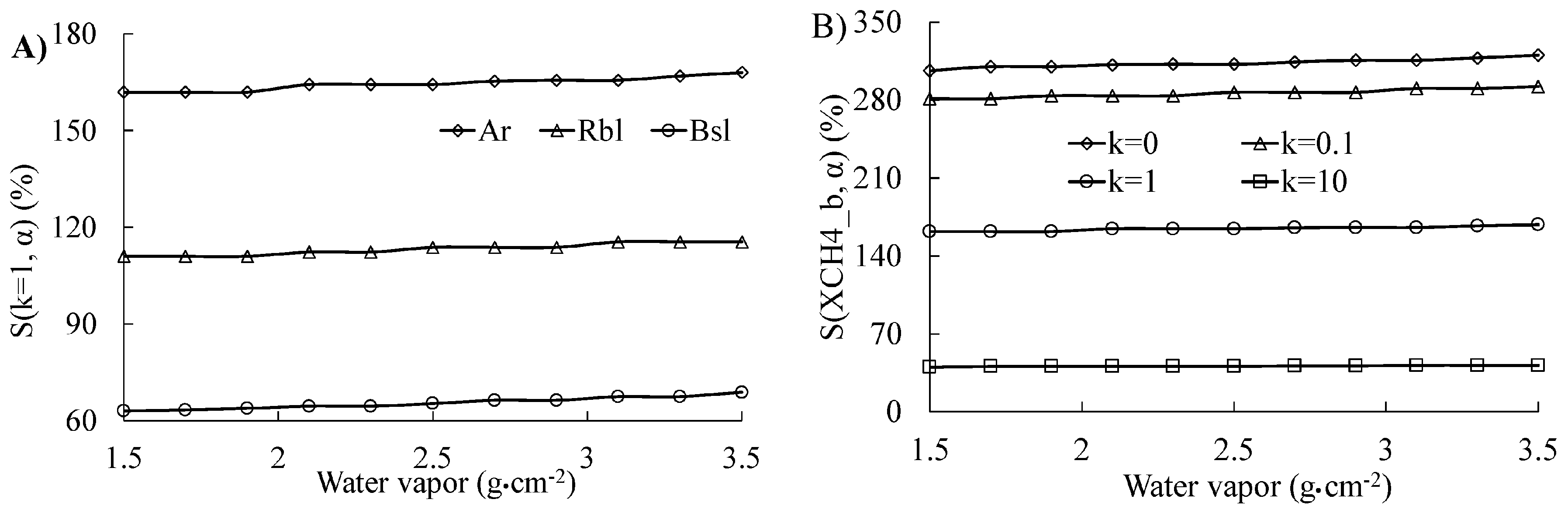
The sensitivity studies showed a significant sensitivity to surface albedo error in retrieved XCH4. We investigated the accuracy of the ρs retrieved from remotely sensed data. An absolute error of 0.02 between MODIS retrieved ρs and in situ data is shown by [43]. Seventy percent of the matchup comparison between MODIS measured and in situ 16-day-averaged ρs from 2001 to 2003 showed an absolute difference of 0.02 [44]. With an assumption that ρs can be retrieved with an absolute error of 0.02 from AVIRIS-NG, the accuracy of AVIRIS-NG retrieved XCH4 was investigated (Figure A4). The S(XCH4_b, α) resulted from an absolute underestimation of 0.02 in ρs can be over 290% for the pixel Ar with a XCH4_A. S(XCH4_b, α) decreases with the increase of ρs and increase of XCH4, to 40% for pixel Ar with a XCH4 plume case of k = 10. The S(XCH4_b, α) decreases slightly with the increase of water vapor.
Figure A4.
S(XCH4_b, α) resulted from an underestimation of 0.02 in ρs for A) three pixels Asphalt road (Ar), Brown sandy loam (Bsl), and Reddish brown sandy loam (Rbl) with the XCH4 plume case of k = 0.1, and B) pixel Ar with XCH4 plume cases of k = 0, 0.1, 1, 10.
Figure A4.
S(XCH4_b, α) resulted from an underestimation of 0.02 in ρs for A) three pixels Asphalt road (Ar), Brown sandy loam (Bsl), and Reddish brown sandy loam (Rbl) with the XCH4 plume case of k = 0.1, and B) pixel Ar with XCH4 plume cases of k = 0, 0.1, 1, 10.

Appendix A.5. Expected Accuracy of AVIRIS-NG Retrieved XCH4
Based on the analysis described above, the accuracy of XCH4 retrieved from a AVIRIS-NG image using the residual radiance method is affected mainly by ρs, although the non-linearity to ρs arises in part from the additive contribution of water vapor column to at sensor radiance. Many algorithms have been developed for retrieving ρs and water vapor from remotely sensed data. The retrieved products have been validated against in situ data, from which the accuracy is derived. With an assumption that ρs and water vapor can be retrieved from AVIRIS-NG imagery with the same accuracy as they are retrieved from remotely sensed data, the expected accuracy for XCH4 retrieved from AVIRIS-NG using the residual radiance method could be derived. An absolute error of 0.02 and a relative error of 9% were selected for the accuracy of ρs and water vapor, respectively.
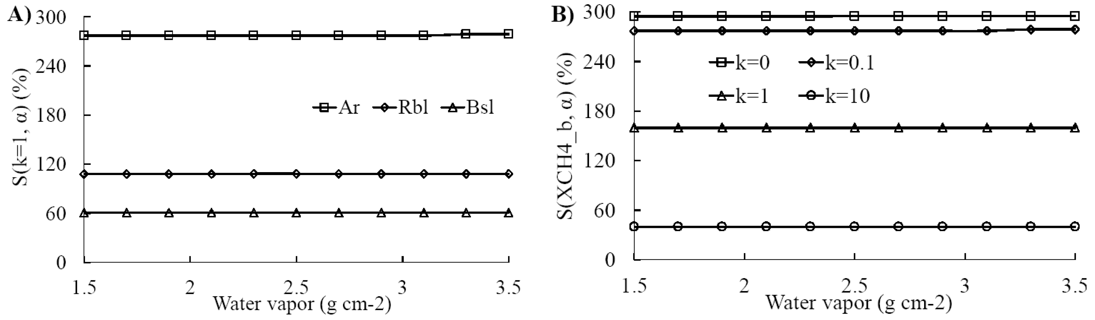
Figure A5 shows the S(XCH4_b, α) resulted from a combination of absolute ρs underestimation of 0.02 and a relative water vapor column overestimation of 9%. The expected accuracy of the XCH4 increases with the increase of XCH4 and the surface albedo. S(XCH4_b, α) is only weakly relate to water vapor column. It should be noted that accuracy is derived without considering the uncertainty in the AVIRIS-NG radiometric calibration and for an assumed NEδL = 0.00035 mW cm−2 μm−1 sr−1. Corrected sensitivities can be derived for improved estimates of uncertainty and NEδL.
Figure A5.
S(XCH4_b, α) resulted from a combination of an absolute underestimation of 0.02 in ρs and a relative overestimation of 9% in column water vapor for (A) three pixels Asphalt road (Ar), Brown sandy loam (Bsl), and Reddish brown sandy loam (Rbl) with the XCH4 plume case of k = 1, and (B) the pixel Ar with XCH4 plume cases of k = 0, 0.1, 1, 10.
References
- IPCC. Climate Change 2013: The Physical Science Basis. Working Group I Contribution to the Fifth Assessment Report of the Intergovernmental Panel on Climate Change; Cambridge University Press: Cambridge, UK, 2014. [Google Scholar]
- Lelieveld, J.O.S.; Crutzen, P.J.; Dentener, F.J. Changing concentration, lifetime and climate forcing of atmospheric methane. Tellus B 1998, 50, 128–150. [Google Scholar] [CrossRef]
- Anderson, B.; Bartlett, K.; Frolking, S.; Hayhoe, K.; Jenkins, J.; Salas, W. Methane and Nitrous Oxide Emissions from Natural Sources; United States Environmental Protection Agency: Washington, DC, USA, 2010.
- Anenberg, S.C.; Schwartz, J.; Shindell, D.; Amann, M.; Faluvegi, G.; Klimont, Z.; Janssens-Maenhout, G.; Pozzoli, L.; Van Dingenen, R.; Vignati, E.; et al. Global air quality and health co-benefits of mitigating near-term climate change through methane and black carbon emission controls. Environ Health Perspect 2012, 120, 831–839. [Google Scholar] [CrossRef] [PubMed] [Green Version]
- Hansen, J.; Sato, M.; Ruedy, R.; Lacis, A.; Oinas, V. Global warming in the twenty-first century: An alternative scenario. Proc. Natl. Acad. Sci. 2000, 97, 9875–9880. [Google Scholar] [CrossRef] [PubMed]
- Nisbet, E.G.; Dlugokencky, E.J.; Bousquet, P. Methane on the rise—again. Science 2014, 343, 493–495. [Google Scholar] [CrossRef] [PubMed] [Green Version]
- Kirschke, S.; Bousquet, P.; Ciais, P.; Saunois, M.; Canadell, J.G.; Dlugokencky, E.J.; Bergamaschi, P.; Bergmann, D.; Blake, D.R.; Bruhwiler, L.; et al. Three decades of global methane sources and sinks. Nat. Geosci. 2013, 6, 813–823. [Google Scholar] [CrossRef]
- Ghosh, A.; Patra, P.K.; Ishijima, K.; Umezawa, T.; Ito, A.; Etheridge, D.M.; Sugawara, S.; Kawamura, K.; Miller, J.B.; Dlugokencky, E.J.; et al. Variations in global methane sources and sinks during 1910–2010. Atmos. Chem. Phys. 2015, 15, 2595–2612. [Google Scholar] [CrossRef]
- Kim, H.-S.; Chung, Y.; Tans, P.; Dlugokencky, E. Decadal trends of atmospheric methane in east asia from 1991 to 2013. Air Qual Atmos Health 2015, 8, 293–298. [Google Scholar] [CrossRef]
- Brandt, A.R.; Heath, G.A.; Kort, E.A.; O’Sullivan, F.; Pétron, G.; Jordaan, S.M.; Tans, P.; Wilcox, J.; Gopstein, A.M.; Arent, D.; et al. Methane leaks from north american natural gas systems. Science 2014, 343, 733–735. [Google Scholar] [CrossRef] [PubMed]
- Miller, S.M.; Wofsy, S.C.; Michalak, A.M.; Kort, E.A.; Andrews, A.E.; Biraud, S.C.; Dlugokencky, E.J.; Eluszkiewicz, J.; Fischer, M.L.; Janssens-Maenhout, G.; et al. Anthropogenic emissions of methane in the united states. Proc. Natl. Acad. Sci. 2013, 110, 20018–20022. [Google Scholar] [CrossRef] [PubMed]
- Dlugokencky, E.J.; Nisbet, E.G.; Fisher, R.; Lowry, D. Global Atmospheric Methane: Budget, Changes and Dangers. Philos. Trans. Soc. A 2011, 369, 2058–2072. [Google Scholar] [CrossRef] [PubMed]
- Buchwitz, M.; Reuter, M.; Bovensmann, H.; Pillai, D.; Heymann, J.; Schneising, O.; Rozanov, V.; Krings, T.; Burrows, J.P.; Boesch, H.; et al. Carbon monitoring satellite (carbonsat): Assessment of atmospheric CO2 and CH4 retrieval errors by error parameterization. Atmos. Meas. Tech. 2013, 6, 3477–3500. [Google Scholar] [CrossRef]
- Buchwitz, M.; Rozanov, V.V.; Burrows, J.P. A near-infrared optimized doas method for the fast global retrieval of atmospheric CH4, CO, CO2, H2O, and N2O total column amounts from sciamachy envisat-1 nadir radiances. J. Geophys. Res. Atmos. 2000, 105, 15231–15245. [Google Scholar] [CrossRef]
- Butz, A.; Hasekamp, O.P.; Frankenberg, C.; Vidot, J.; Aben, I. CH4 retrievals from space-based solar backscatter measurements: Performance evaluation against simulated aerosol and cirrus loaded scenes. J. Geophys. Res. Atmos. 2010, 115, D24302. [Google Scholar] [CrossRef]
- Kuze, A.; Suto, H.; Nakajima, M.; Hamazaki, T. Thermal and near infrared sensor for carbon observation fourier-transform spectrometer on the greenhouse gases observing satellite for greenhouse gases monitoring. Appl. Optics 2009, 48, 6716–6733. [Google Scholar] [CrossRef] [PubMed]
- Schepers, D.; Guerlet, S.; Butz, A.; Landgraf, J.; Frankenberg, C.; Hasekamp, O.; Blavier, J.F.; Deutscher, N.M.; Griffith, D.W.T.; Hase, F.; et al. Methane retrievals from greenhouse gases observing satellite (gosat) shortwave infrared measurements: Performance comparison of proxy and physics retrieval algorithms. J. Geophys. Res. Atmos. 2012, 117, D10307. [Google Scholar] [CrossRef]
- Veefkind, J.P.; Aben, I.; McMullan, K.; Förster, H.; de Vries, J.; Otter, G.; Claas, J.; Eskes, H.J.; de Haan, J.F.; Kleipool, Q.; et al. Tropomi on the esa sentinel-5 precursor: A gmes mission for global observations of the atmospheric composition for climate, air quality and ozone layer applications. Remote Sens. Environ. 2012, 120, 70–83. [Google Scholar] [CrossRef]
- Krings, T.; Gerilowski, K.; Buchwitz, M.; Hartmann, J.; Sachs, T.; Erzinger, J.; Burrows, J.P.; Bovensmann, H. Quantification of methane emission rates from coal mine ventilation shafts using airborne remote sensing data. Atmos. Meas. Tech. 2013, 6, 151–166. [Google Scholar] [CrossRef] [Green Version]
- Tratt, D.M.; Buckland, K.N.; Hall, J.L.; Johnson, P.D.; Keim, E.R.; Leifer, I.; Westberg, K.; Young, S.J. Airborne visualization and quantification of discrete methane sources in the environment. Remote Sens. Environ. 2014, 154, 74–88. [Google Scholar] [CrossRef]
- Kuai, L.; Worden, J.R.; Li, K.; Hulley, G.C.; Hopkins, F.M.; Miller, C.E.; Hook, S.J.; Duren, R.M.; Aubrey, A.D. Characterization of anthropogenic methane plumes with the hyperspectral thermal emission spectrometer (hytes): A retrieval method and error analysis. Atmos. Meas. Tech. Discuss. 2016, 2016, 1–24. [Google Scholar] [CrossRef]
- Thorpe, A.K.; Frankenberg, C.; Roberts, D.A. Retrieval techniques for airborne imaging of methane concentrations using high spatial and moderate spectral resolution: Application to aviris. Atmos. Meas. Tech. 2014, 7, 491–506. [Google Scholar] [CrossRef]
- Thompson, D.R.; Leifer, I.; Bovensmann, H.; Eastwood, M.; Fladeland, M.; Frankenberg, C.; Gerilowski, K.; Green, R.O.; Kratwurst, S.; Krings, T.; et al. Real-time remote detection and measurement for airborne imaging spectroscopy: A case study with methane. Atmos. Meas. Tech. 2015, 8, 4383–4397. [Google Scholar] [CrossRef]
- Bradley, E.S.; Leifer, I.; Roberts, D.A.; Dennison, P.E.; Washburn, L. Detection of marine methane emissions with aviris band ratios. Geophys. Res. Lett. 2011, 38, L10702. [Google Scholar] [CrossRef]
- Thorpe, A.K.; Roberts, D.A.; Bradley, E.S.; Funk, C.C.; Dennison, P.E.; Leifer, I. High resolution mapping of methane emissions from marine and terrestrial sources using a cluster-tuned matched filter technique and imaging spectrometry. Remote Sens. Environ. 2013, 134, 305–318. [Google Scholar] [CrossRef]
- Frankenberg, C.; Meirink, J.F.; van Weele, M.; Platt, U.; Wagner, T. Assessing methane emissions from global space-borne observations. Science 2005, 308, 1010–1014. [Google Scholar] [CrossRef] [PubMed]
- Washburn, L.; Clark, J.F.; Kyriakidis, P. The spatial scales, distribution, and intensity of natural marine hydrocarbon seeps near coal oil point, california. Mar. Petroleum Geology 2005, 22, 569–578. [Google Scholar] [CrossRef]
- Leifer, I.; Melton, C.; Fischer, M.L.; Fladeland, M.; Frash, J.; Gore, W.; Iraci, L.; Marrero, J.; Ryoo, J.M.; Tanaka, T.; et al. Improved atmospheric characterization through fused mobile airborne & surface in situ surveys: Methane emissions quantification from a producing oil field. Atmos. Meas. Tech. Discuss. 2017, 2017, 1–30. [Google Scholar]
- Roberts, D.A.; Bradley, E.S.; Cheung, R.; Leifer, I.; Dennison, P.E.; Margolis, J.S. Mapping methane emissions from a marine geological seep source using imaging spectrometry. Remote Sens. Environ. 2010, 114, 592–606. [Google Scholar] [CrossRef]
- Green, R.O.; Eastwood, M.L.; Sarture, C.M.; Chrien, T.G.; Aronsson, M.; Chippendale, B.J.; Faust, J.A.; Pavri, B.E.; Chovit, C.J.; Solis, M.; et al. Imaging spectroscopy and the airborne visible/infrared imaging spectrometer (aviris). Remote Sens. Environ. 1998, 65, 227–248. [Google Scholar] [CrossRef]
- Hamlin, L.; Green, R.O.; Mouroulis, P.; Eastwood, M.; Wilson, D.; Dudik, M.; Paine, C. Imaging spectrometer science measurements for terrestrial ecology: AVIRIS and new developments. In NASA Earth Science Technology Forum; Jet Propul. Lab: Paseda, CA, USA, 2010. [Google Scholar]
- Dennison, P.E.; Thorpe, A.K.; Pardyjak, E.R.; Roberts, D.A.; Qi, Y.; Green, R.O.; Bradley, E.S.; Funk, C.C. High spatial resolution mapping of elevated atmospheric carbon dioxide using airborne imaging spectroscopy: Radiative transfer modeling and power plant plume detection. Remote Sens. Environ. 2013, 139, 116–129. [Google Scholar] [CrossRef]
- Green, R.O.; Pavri, B. Aviris Inflight Calibration Experiment Measurements, Analyses, and Results in 2000. In Proceedings of the Tenth JPL Airvorne Earth Science Workshop, Pasadena, CA, USA, 5–8 March 2002. [Google Scholar]
- Krautwurst, S.; Gerilowski, K.; Krings, T.; Borchard, J.; Bovensmann, H. COMEX—Final Report. Available online: https://espo.nasa.gov/missions/sites/default/files/documents/COMEX_FR_v2.0_final_.pdf (accessed on 12 August 2017).
- Kaufman, Y.J.; Bo-Cai, G. Remote sensing of water vapor in the near ir from eos/modis. IEEE Trans. Geosci. Remote Sens. 1992, 30, 871–884. [Google Scholar] [CrossRef]
- Albert, P.; Bennartz, R.; Preusker, R.; Leinweber, R.; Fischer, J. Remote sensing of atmospheric water vapor using the moderate resolution imaging spectroradiometer. J. Atmos. Ocean. Technol. 2005, 22, 309–314. [Google Scholar] [CrossRef]
- HyspIRI. Hyspiri Mission Study Website. Available online: http://hyspiri.jpl.nasa.gov/ (accessed on 6 March 2011).
- Noël, S.; Bramstedt, K.; Bovensmann, H.; Gerilowski, K.; Burrows, J.P.; Standfuss, C.; Dufour, E.; Veihelmann, B. Quantification and mitigation of the impact of scene inhomogeneity on sentinel-4 uvn uv-vis retrievals. Atmos. Meas. Tech. 2012, 5, 1319–1331. [Google Scholar] [CrossRef]
- Cirpas, the Center for Interdisciplinary Remotely-Piloted Aircraft Studies. Available online: www.cirpas.org (accessed on 1 November 2014).
- Sweet, J.N. The Spectral Similarity Scale and Its Application to the Classification of Hyperspectral Remote Sensing Data. In Proceedings of the 2003 IEEE Workshop on Advances in Techniques for Analysis of Remotely Sensed Data, Greenbelt, MD, USA, 27–28 Octomber 2003. [Google Scholar]
- Morino, I.; Uchino, O.; Inoue, M.; Yoshida, Y.; Yokota, T.; Wennberg, P.O.; Toon, G.C.; Wunch, D.; Roehl, C.M.; Notholt, J.; et al. Preliminary validation of column-averaged volume mixing ratios of carbon dioxide and methane retrieved from GOSAT short-wavelength infrared spectra. Atmos. Meas. Tech. 2011, 4, 1061–1076. [Google Scholar] [CrossRef]
- Butz, A.; Guerlet, S.; Hasekamp, O.; Schepers, D.; Galli, A.; Aben, I.; Frankenberg, C.; Hartmann, J.M.; Tran, H.; Kuze, A.; et al. Toward accurate CO2 and CH4 observations from gosat. Geophys. Res. Lett. 2011, 38, L14812. [Google Scholar] [CrossRef]
- Privette, J.L.; Mukelabai, M.; Zhang, H.; Schaaf, C.B. Characterization of MODIS land albedo (mod43) accuracy with atmospheric conditions in Africa. In Proceedings of the 2004 IEEE International Geoscience and Remote Sensing Symposium, Anchorage, AK, USA, 20–24 September 2004. [Google Scholar]
- Wang, K.; Liu, J.; Zhou, X.; Sparrow, M.; Ma, M.; Sun, Z.; Jiang, W. Validation of the modis global land surface albedo product using ground measurements in a semidesert region on the tibetan plateau. J. Geophys. Res. Atmos. 2004, 109, D05107. [Google Scholar] [CrossRef]
Figure 1.
(A) True color imagery of Airborne Visual Infrared Imaging Spectrometer-Classic (AVIRIS-C) data acquired on 19 June 2008. (B) Band ratio (σ) of at-sensor reflectance (ρt) for the 2298 and 2058 nm bands, σ = ρt(2298)/ρt(2058) for AVIRIS-C data in (A), black rectangle outline shows clear plume structure. (C) True color imagery of AVIRIS-C data acquired on 6 June 2013. (D) σ for AVIRIS-C data in (C). Data key on figure.

Figure 2.
True color imagery for AVIRIS-NG image of the Kern Front oil field, near Bakersfield, central California on 4 September 2014. The land cover types for the three pixels selected for sensitivity analysis are noted, by Ar, Bsl, and Rbl, which are for Asphalt road, Brown sandy loam, and Reddish brown sandy loam, respectively. Pixels in the red box are used to investigate the effect of subpixel heterogeneity on albedo and XCH4.
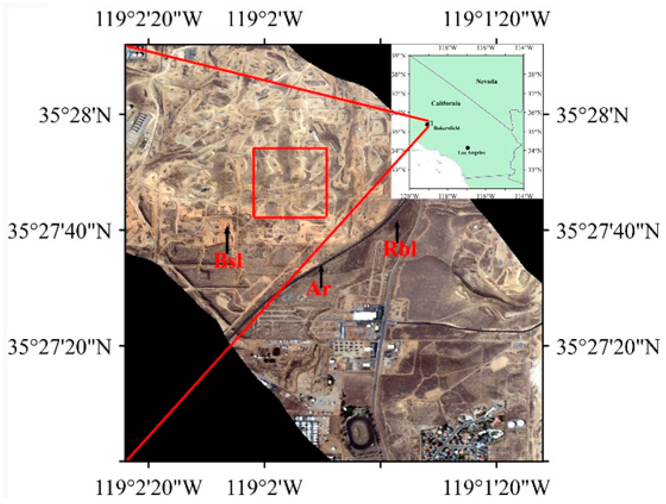
Figure 3.
(A) In situ methane, CH4, and wind data for 4 September 2014 collected by CIRPAS for the Kern Front and Kern River oil fields. Data key on panel. (B) Derived in situ and uniform CH4 profiles, which have the same column-averaged CH4 within a boundary layer of 2.0 km.
Figure 3.
(A) In situ methane, CH4, and wind data for 4 September 2014 collected by CIRPAS for the Kern Front and Kern River oil fields. Data key on panel. (B) Derived in situ and uniform CH4 profiles, which have the same column-averaged CH4 within a boundary layer of 2.0 km.
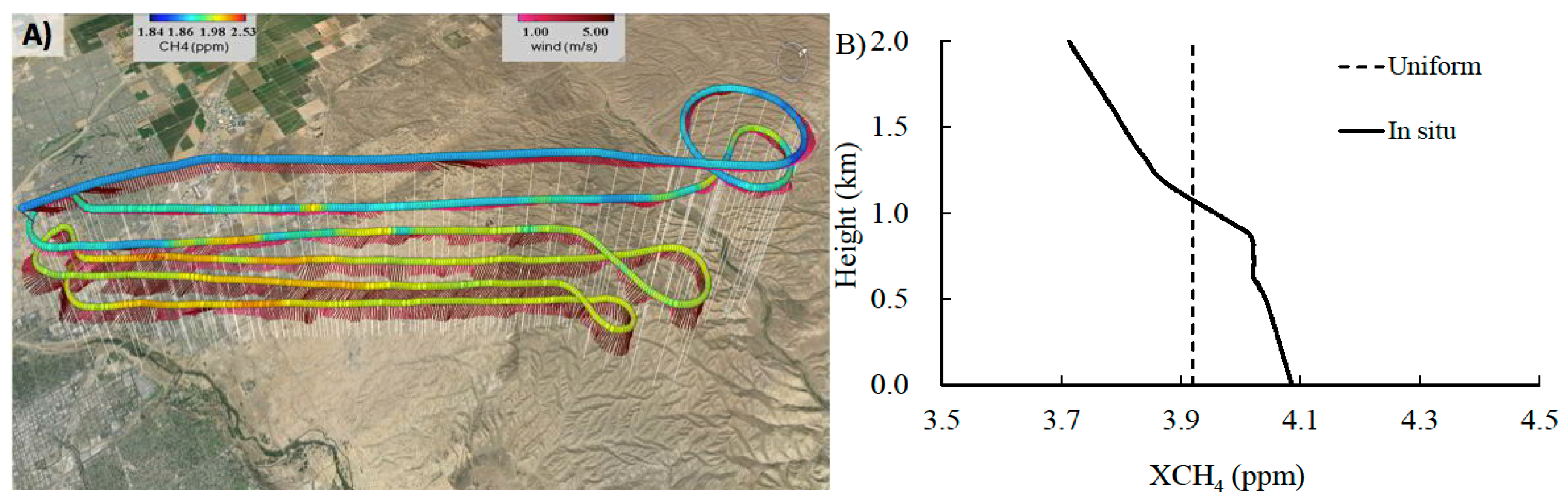
Figure 4.
Transmittance spectra for H2O and CH4 in wavelength ranges of (A) 1600–2500 nm, (B) 2239–2299 nm, generated using MODerate resolution atmospheric correction TRANsmission (MODTRAN) for a mid-latitude summer atmosphere for the AVIRIS-NG sensor (Figure 2) at 2.4 km altitude with CH4 based on in situ data, see Figure 3.

Figure 5.
Surface albedo (ρs) for (A) 500 to 2500 nm, (B) 2139 to 2299 nm, for three common scene elements: asphalt road (Ar), brown sandy loam (Bsl), and red-brown sandy loam (Rbl), respectively. Data key on figure. Spectra are from Environment for Visualizing Images (ENVI) library.
Figure 5.
Surface albedo (ρs) for (A) 500 to 2500 nm, (B) 2139 to 2299 nm, for three common scene elements: asphalt road (Ar), brown sandy loam (Bsl), and red-brown sandy loam (Rbl), respectively. Data key on figure. Spectra are from Environment for Visualizing Images (ENVI) library.

Figure 6.
(A) Relative error (β) in at sensor radiance (Lt(λ)) with respect to the relative surface albedo error (α) and 1:1 line (solid). (B) Relative methane column, XCH4, sensitivity, S(XCH4_b, α) with respect to α for the three land cover types, Ar, Bsl, Rbl, which are for Asphalt road, Brown sandy loam, and Reddish brown sandy loam, respectively. XCH4_b is for the observed plume (k = 1) in all simulations. (C) S(XCH4_b, α) for pixel Rbl with different plume strength cases defined by k, see Equation (4). (D) Expanded view of (C) for positive α.
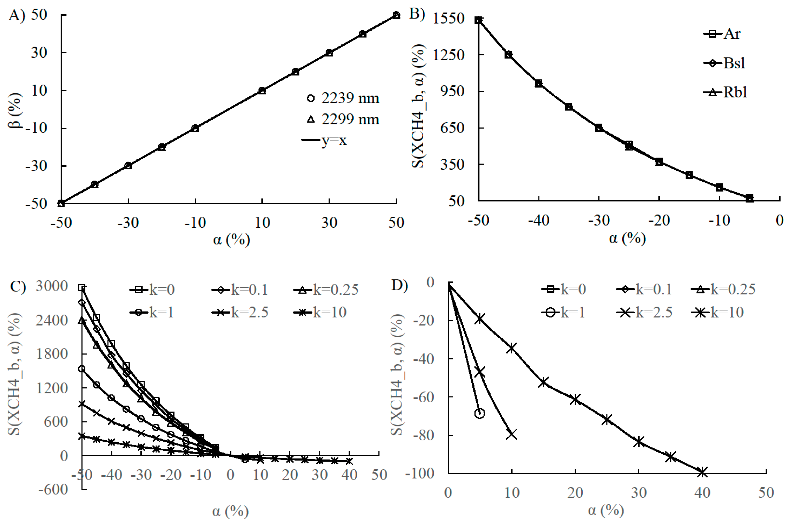
Figure 7.
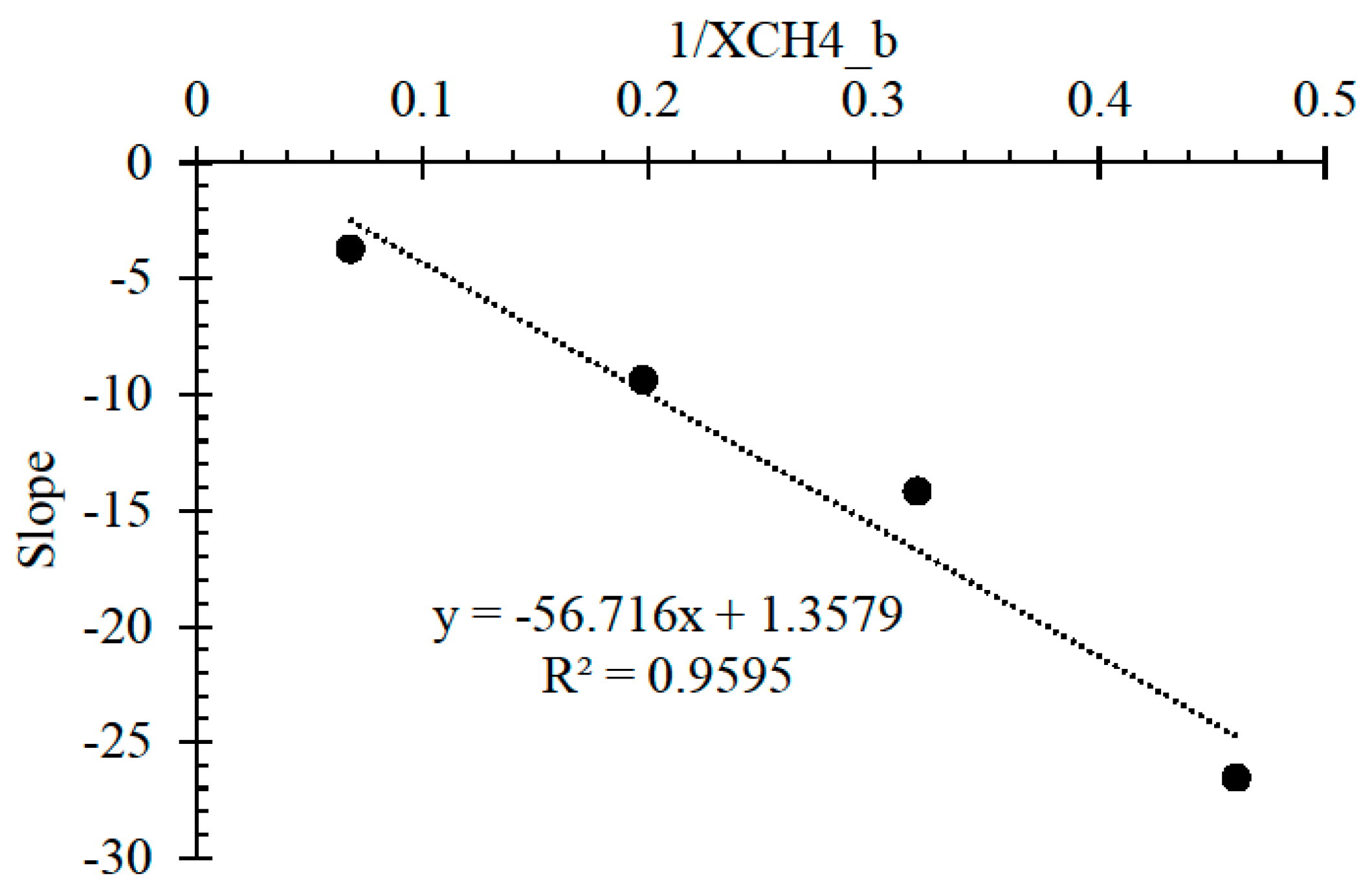
Inverse XCH4_b (1/XCH4_b) versus slope of the lines in Figure 6C, calculated for data near α = 0 for the plume strength cases of k = 0.25, 1, 2.5, and 10.
Figure 7.
Inverse XCH4_b (1/XCH4_b) versus slope of the lines in Figure 6C, calculated for data near α = 0 for the plume strength cases of k = 0.25, 1, 2.5, and 10.

Figure 8.
Introduced relative error(SUni/SObs), for two scenarios, a uniform 2.0 km planetary boundary layer (PBL) (SUni) relative to the observed profile (SObs) shown in Figure 3. Both scenarios have the same XCH4.
Figure 8.
Introduced relative error(SUni/SObs), for two scenarios, a uniform 2.0 km planetary boundary layer (PBL) (SUni) relative to the observed profile (SObs) shown in Figure 3. Both scenarios have the same XCH4.
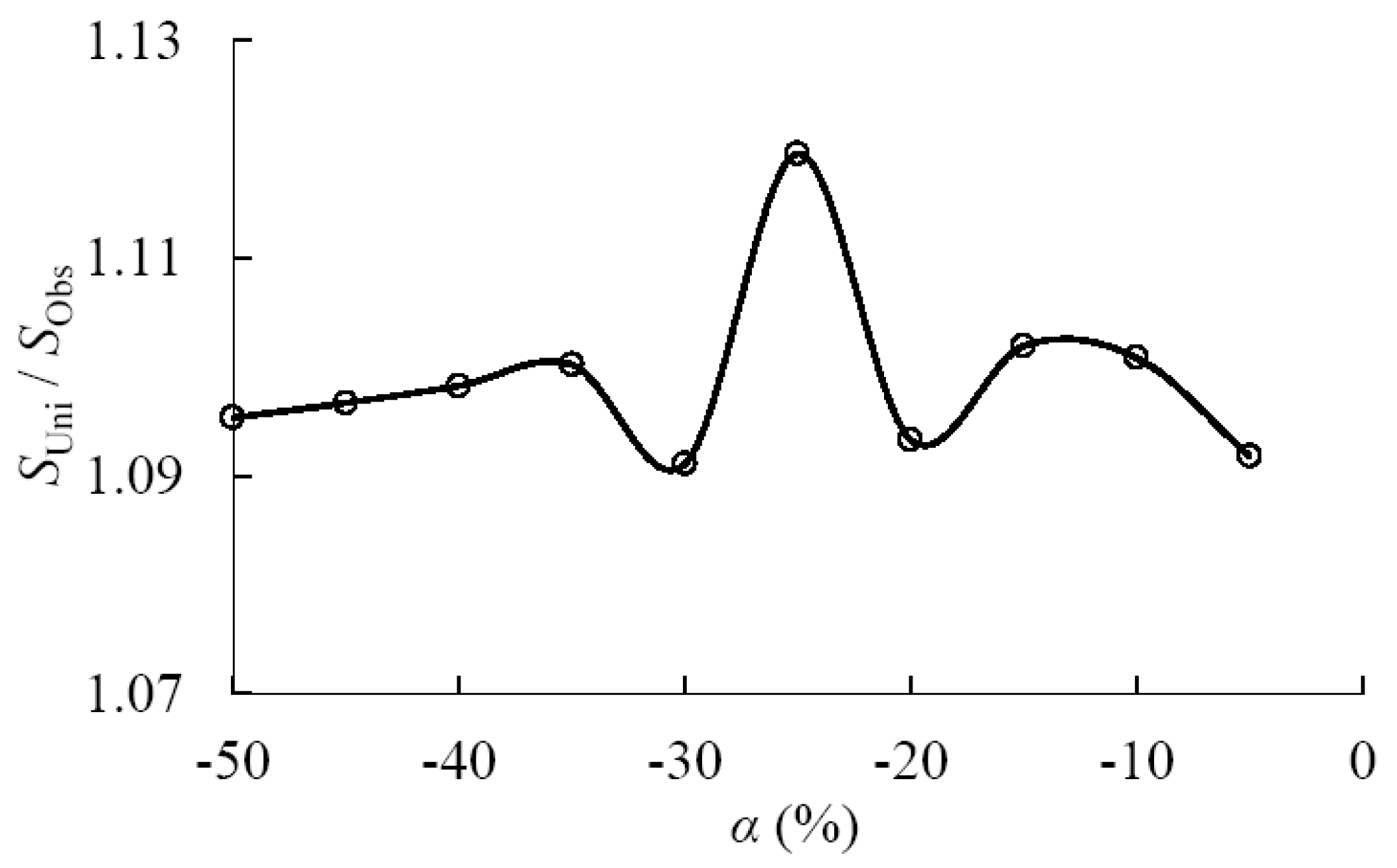
Figure 9.
Column retrieval error (S(k = 1, α = −10%)) where k = 1 signifies the plume profile (Figure 3) for (A) solar zenith angle (θs) when viewing zenith angle (θv) and relative sun-senor azimuth angle (φ) are equal to 8°, 90° respectively, (B) θv when θs and φ are equal to 40°, 90° respectively, and (C) φ when θs and θv are equal to 40°, 8° respectively.

Figure 10.
Column retrieval error (S(XCH4_b, α)) versus α for XCH4_b of plume case k = 1 for (A) different aerosol type, (B) different visibility.
Figure 10.
Column retrieval error (S(XCH4_b, α)) versus α for XCH4_b of plume case k = 1 for (A) different aerosol type, (B) different visibility.

Figure 11.
Calculated sensor radiance (Lt) with respect to wavelength (λ)simulated for background XCH4. Solid lines show Lt for the true ρs(λ) (denoted “_True”) for spectra for scene elements Asphalt road (Ar), Brown sandy loam (Bsl), and Reddish-brown fine sandy loam (Rbl) shown in Figure 3. Dashed lines show Lt for constant ρs(2139) across the feature (denoted “_Flat”).

Figure 12.
S(XCH4_b, α = 0) resulting from an overestimation of 9% in water vapor for (A) three pixels types, Asphalt road (Ar), Brown sandy loam (Bsl), and Reddish-brown sandy loam (Rbl) with the XCH4 plume case, defined as k = 1, and (B) the pixel Ar for different XCH4 plume strengths k = 0, 0.1, 0.25, 1, 2.5, 10. k = 0 represents background.

Figure 13.
Lt_OA derived by averaging Lt simulated over each subpixel (a total of 160 × 160 subpixels), see text for description. Lt_AO simulated using the average albedo of the 160 × 160 subpixels. GOSAT pixel noted above. In situ profile (i.e., k = 1, Figure 3) was used for calculating Lt_OA and Lt_AO.

Figure 14.
XCH4 underestimation (γ) with the subpixel percent coverage (Pc) of the GOSAT pixel covered by a CH4 plume anomalies from 0.05 to 1 ppm, remainder background CH4. Data key on figure.
Figure 14.
XCH4 underestimation (γ) with the subpixel percent coverage (Pc) of the GOSAT pixel covered by a CH4 plume anomalies from 0.05 to 1 ppm, remainder background CH4. Data key on figure.
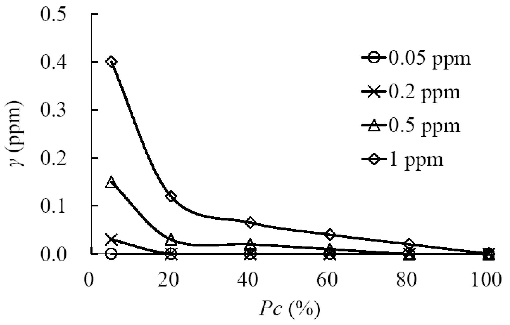
Table 1.
Nomenclature.
| Symbol | Definition | Unit |
|---|---|---|
| Ar | Asphalt road | N/A |
| Bsl | Brown sandy loam | N/A |
| Rbl | Reddish-brown fine sandy loam | N/A |
| GOSAT | Greenhouse gases Observing SATellite | N/A |
| i | Band number | N/A |
| k | Scaling factor forXCH4_p | N/A |
| Lt(α, λ) | at-sensor radiance in wavelength λ for a ρs relative error of α | mW cm−2 μm−1 sr−1 |
| S(XCH4_b, α) | Albedo sensitivity with a scenario, XCH4_b and the relative error, α, in ρs | dimensionless |
| XCH4 | Methane column ratio | ppm |
| XCH4_A | Background methane column ratio | ppm |
| XCH4_P | Plume methane column ratio | ppm |
| XCH4_b | Base XCH4 | ppm |
| XCH4_err | XCH4 from trial and error | ppm |
| XCH4_GOSAT | Mean XCH4 over subpixels in GOSAT pixel | ppm |
| θs | Solar zenith angle | degree |
| θv | Viewing zenith angle | degree |
| ϕ | Relative sun-sensor azimuth angle | degree |
| λ | Wavelength | nm |
| ρs(λ) | Surface albedo | dimensionless |
| ρt(λ) | At-sensor reflectance | dimensionless |
| Lt(λ) | At-sensor radiance | mW cm−2 μm−1 sr−1 |
| Lt_GOSAT(λ) | Mean Lt(λ) over subpixels in GOSAT pixel | mW cm−2 μm−1 sr−1 |
| Lt_AO(λ) | Mean Lt over the subpixels | mW cm−2 μm−1 sr−1 |
| Lt_OA(λ) | Lt for the mean surface albedo over subpixels | mW cm−2 μm−1 sr−1 |
| Lt_err | Lt for the original albedo and XCH4 with 10% underestimation | mW cm−2 μm−1 sr−1 |
| ρs_err | ρs corresponding to Lt_err and the original XCH4 | dimensionless |
| XCH4_M | XCH4 corresponding to Lt_GOSAT and mean albedo over GOSAT subpixels | ppm |
| NEδL | Noise equivalent delta radiance | mW cm−2 μm−1 sr−1 |
| NEδLa | NEδL adjusted to the band average | mW cm−2 μm−1 sr−1 |
| α | Relative error in surface albedo | % |
| β | Relative error in Lt | % |
| γ | Underestimate of XCH4 resulted from the subpixel heterogeneity of CH4 | ppm |
| σ | ρt(2298)/ρt(2058) | dimensionless |
| Δ | Average residual radiance | mW cm−2 μm−1 sr−1 |
| Pc | Percentage of area in one GOSAT pixel covered by XCH4 plume | % |
Table 2.
S(XCH4_b, α = 0) resulting from constant ρs assumption for wavelengths 2239 to 2299 nm.
| XCH4_b | Underestimation (%) | ||
|---|---|---|---|
| Ar | Rbl | Bsl | |
| k = 0 | - | −79.77 | −73.72 |
| k = 0.1 | −120.73 | −70.35 | −63.97 |
| k = 1 | −79.68 | −35.81 | −30.95 |
| k = 10 | −30.18 | −10.65 | −8.08 |
© 2017 by the authors. Licensee MDPI, Basel, Switzerland. This article is an open access article distributed under the terms and conditions of the Creative Commons Attribution (CC BY) license (http://creativecommons.org/licenses/by/4.0/).
Share and Cite
MDPI and ACS Style
Zhang, M.; Leifer, I.; Hu, C. Challenges in Methane Column Retrievals from AVIRIS-NG Imagery over Spectrally Cluttered Surfaces: A Sensitivity Analysis. Remote Sens. 2017, 9, 835. https://doi.org/10.3390/rs9080835
AMA Style
Zhang M, Leifer I, Hu C. Challenges in Methane Column Retrievals from AVIRIS-NG Imagery over Spectrally Cluttered Surfaces: A Sensitivity Analysis. Remote Sensing. 2017; 9(8):835. https://doi.org/10.3390/rs9080835
Chicago/Turabian StyleZhang, Minwei, Ira Leifer, and Chuanmin Hu. 2017. "Challenges in Methane Column Retrievals from AVIRIS-NG Imagery over Spectrally Cluttered Surfaces: A Sensitivity Analysis" Remote Sensing 9, no. 8: 835. https://doi.org/10.3390/rs9080835
Note that from the first issue of 2016, this journal uses article numbers instead of page numbers. See further details here.