
Assimilation of Sentinel-1 Derived Sea Surface Winds for Typhoon Forecasting


1
School of Computer Science, National University of Defense Technology, Changsha 410073, China
2
State Key Laboratory of Remote Sensing Science, Institute of Remote Sensing and Digital Earth, Chinese Academy of Sciences, Beijing 100101, China
3
The Key Laboratory for Earth Observation of Hainan Province, Sanya 572029, China
*
Author to whom correspondence should be addressed.
Remote Sens. 2017, 9(8), 845; https://doi.org/10.3390/rs9080845
Submission received: 16 June 2017
/
Revised: 9 August 2017
/
Accepted: 10 August 2017
/
Published: 14 August 2017
(This article belongs to the Special Issue Ocean Remote Sensing with Synthetic Aperture Radar)
Abstract
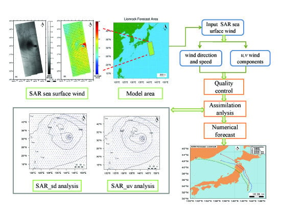
:High-resolution synthetic aperture radar (SAR) wind observations provide fine structural information for tropical cycles and could be assimilated into numerical weather prediction (NWP) models. However, in the conventional method assimilating the u and v components for SAR wind observations (SAR_uv), the wind direction is not a state vector and its observational error is not considered during the assimilation calculation. In this paper, an improved method for wind observation directly assimilates the SAR wind observations in the form of speed and direction (SAR_sd). This method was implemented to assimilate the sea surface wind retrieved from Sentinel-1 synthetic aperture radar (SAR) in the basic three-dimensional variational system for the Weather Research and Forecasting Model (WRF 3DVAR). Furthermore, a new quality control scheme for wind observations is also presented. Typhoon Lionrock in August 2016 is chosen as a case study to investigate and compare both assimilation methods. The experimental results show that the SAR wind observations can increase the number of the effective observations in the area of a typhoon and have a positive impact on the assimilation analysis. The numerical forecast results for this case show better results for the SAR_sd method than for the SAR_uv method. The SAR_sd method looks very promising for winds assimilation under typhoon conditions, but more cases need to be considered to draw final conclusions.
1. Introduction
Sea surface wind is the primary power source for atmospheric movement over the ocean surface [1] and remarkably affects the air-sea exchange process. Tropical cyclones (TCs), storm surges, and many other severe ocean conditions are driven by the sea surface wind. However, the usual measurements of sea surface wind observations from the buoys and ships are scarce and distributed irregularly. The observations for bad weather are often far away from ships on limited routes, and especially, there are few observations of high precision and resolution in the area of TCs. The lack of observations regarding the initial analysis in the TC model would greatly reduce the accuracy of the TC forecast.
In recent years, microwave remote sensing instruments such as microwave scatterometers and synthetic aperture radar (SAR) have been used to retrieve sea surface wind fields [2,3,4]. Although the scatterometer observes the ocean surface with wide coverage [5], the spatial resolution of scatterometers is 12.5~25 km and the accuracy of scatterometers’ measurements of winds is low in coastal regions [6]. However, the SAR observations are of high spatial resolution [7,8,9], and these data can provide very detailed information on the structure of tropical cyclones [10]. The accuracy of sea surface wind data retrieved from SAR is also comparable with scatterometer data [11,12], and these wind fields can be used with a data assimilation system to provide the initial conditions for the numerical weather prediction (NWP) model [13]. Some researchers have tried to adopt the SAR observations in the assimilation system. Danielson designed a plan to assimilate SAR wind information in Environment Canada’s high-resolution three-dimensional variational (3DVAR) analysis system [14]. Perrie et al. assimilated the SAR derived wind, which captured Hurricane Isanbe’eye, and found that the analysis from the experiment provided new information about Isabel’s central region [15]. Choisnard et al. assessed the quality of a marine wind vector retrieved from the variational data assimilation of SAR backscatter observation and inferred that wind direction information from wind streaks could be of interest to add some wind direction sensitivity [16].
The SAR derived wind products are in the form of the wind speed (spd) and the wind direction (dir). In current data assimilation systems, including the Weather Research and Forecasting Model Data Assimilation system (WRFDA), the input wind products are transformed to a longitudinal component (u wind) and a latitudinal component (v wind). Then, u and v are used in the assimilation calculation as the vectors for wind observations [17]. In this conventional method, dir is not a state vector and can not influence the analysis directly. Furthermore, the impact of the dir observational error on u and v is ignored. This will cause large errors in the u and v assimilation, especially when the wind observations are largely different from the background wind, e.g., during typhoon events [18]. In fact, for SAR wind retrieval, the wind speed is derived from the radar sea surface backscattering signal, while the wind direction is usually extracted from wind-aligned patterns on SAR imagery [10]. Consequently, the spd and dir errors of SAR observations are independent, and the dir observational error should not be ignored in the wind data assimilation.
Recently, a novel method to assimilate the wind observations has been proposed by Huang et al., which directly assimilates spd and dir based on the transformation of the state vectors u and v to spd and dir by the observation operator [18]. Gao et al. further tested this method in the experiments for the satellite-derived Atmospheric Motion Vectors (AMV) and the surface dataset in the Meteorological Assimilation Data Ingest System (MADIS) [19]. However, the quality control process is ignored for the ideal observations in these studies, and the derived values of u and v were not checked together in the quality control stage, even though they were derived from a single wind vector. In this study, an improved method is proposed based on Huang et al., which can assimilate the SAR wind data under typhoon conditions. A new quality control scheme is also presented. The proposed methods are tested and compared with the traditional methods within the WRF/3DVAR framework for the prediction of Typhoon Lionrock (2016). The impact of assimilation of SAR sea surface winds on the typhoon track and intensity will be examined using different methods.
The rest of the paper is organized as follows. In Section 2, we introduce the sea surface wind retrieval method, the assimilation methods, and the quality control scheme. The numerical model and experiment setup are described in Section 3. The experimental results are compared and discussed in Section 4. The conclusions are presented in Section 5.
2. Data and Methodology
2.1. SAR Wind Retrieval
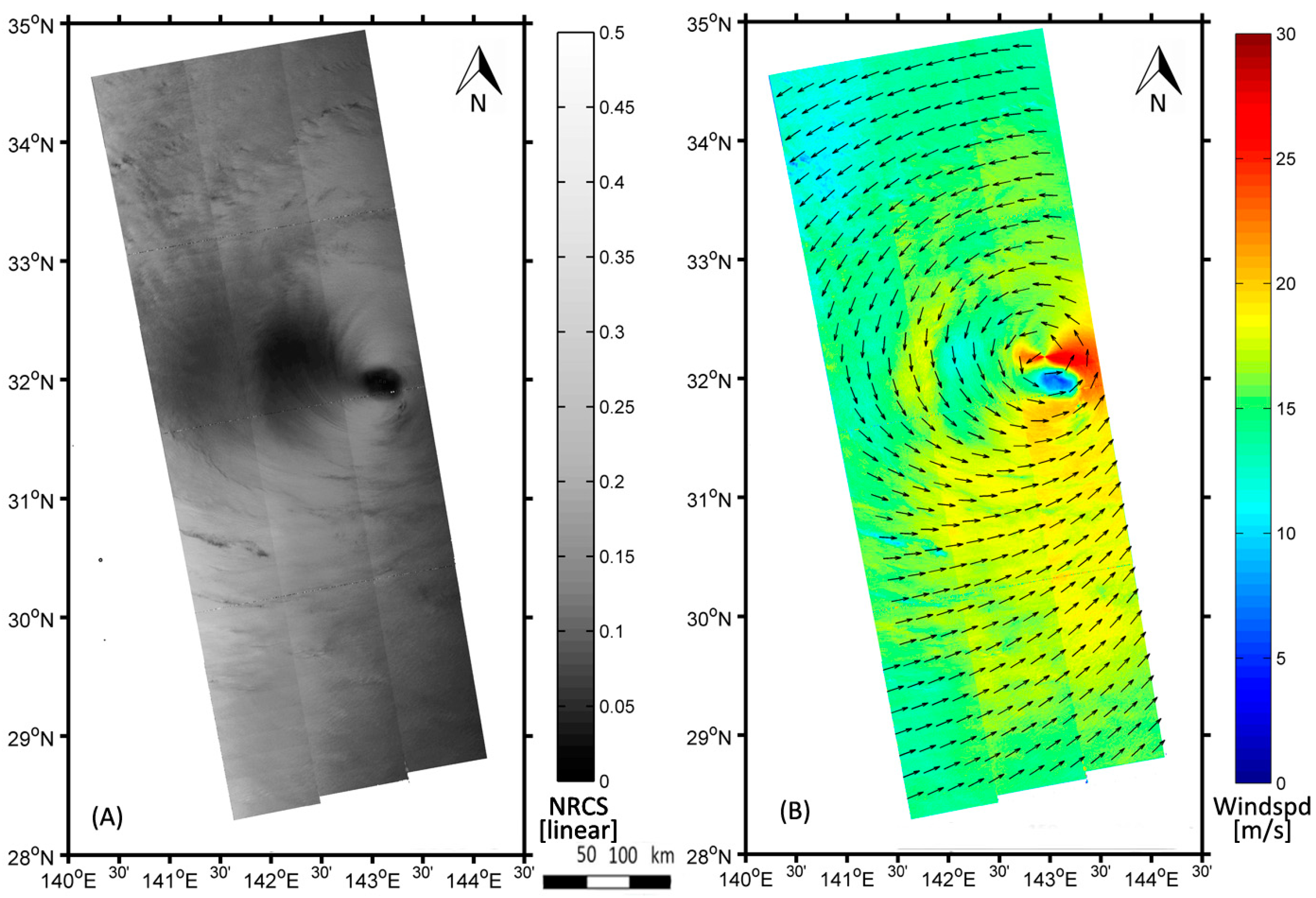
On 3 April 2014, the European Space Agency (ESA) launched the C-band Sentinel-1A satellite. They acquired the first Sentinel-1 typhoon image in the northwest Pacific on 4 October 2014 [20]. Sentinel-1 provides free and open SAR data for ocean, land changes, and emergency response applications, and the data have been utilized in research for hurricane/typhoon studies [21,22,23]. Sentinel-1 has four operational modes, i.e., Strip Map Mode, Interferometric Wide Swath Mode, Extra-wide Swath Mode, and Wave Mode. Sentinel-1 has selectable single polarization (VV, vertical transmit and vertical receive or HH, horizontal transmit and horizontal receive) for the Wave Mode and selectable dual polatization (VV + VH, vertical transmit and horizontal receive or HH + HV, horizontal transmit and vertical receive) for all other modes. In this study, an Extra-wide Swath Mode dual polarization (VV + VH) SAR image is used to derive the sea surface wind map of Typhoon Lionrock (as shown in Figure 1). Its swath is 400 km, and its spatial resolution is 25 × 100 m.
The raw data of Sentinel-1 observations are first calibrated to give the Normalized Radar Cross-section (NRCS), which expresses the radar return signal per unit area and depends on the instant wind stress over the ocean surface and the radar viewing geometry. The Geophysic model function (GMF) is used for SAR wind retrieval and here a C-band geophysical model function (CMOD-5) [24] is used to convert the calibrated NRCS measurement to sea surface winds. The general form of the GMF is:
where is NRCS; is the wind speed at 10 m; is the wind direction with respect to the radar look direction; is local incidence angle; is the method of polarization; and is the frequency of the incident radar wave. As shown in Equation (1), the wind speed retrieval from SAR requires a priori information about the wind direction as the SAR is only capable of observing each point on the ocean surface from a single look angle. This wind direction information is usually obtained from in situ measurements, numerical model outputs, or SAR imagery. For the typhoon wind field, there are wind streaks in SAR imagery, and the wind direction can be extracted from this image pattern. In this study, a method called Discrete Wavelet Transform (DWT) is chosen to derive the sea surface wind direction. The details of the DWT methods can be found in Du et al., 2002 [25] and Zhou et al., 2013 [26]. In the SAR wind retrieval, the heavy rain has been filtered out.
2.2. Data Assimilationof SAR Sea Surface Winds
Data assimilation provides initial conditions to atmospheric models by concentrating on searching for a solution that minimizes simultaneously the distance between observations and the background and the distance between the initial guess variables and the analysis variables [27]. In the three dimensional variational data assimilation (3DVAR) framework, the initial conditions are the best estimations obtained through the minimization of a cost function based on Bayes theory [28], defined as:
Here, is the background term and describes the misfit between the model state variable x and the background state , which is derived from short-range forecast. is the observation term, describing the misfit between the observation vector and the vector equivalent to the model state variable, which is projected to the observation space by the observation operator H [29,30]. B and R are the background and observational error covariance matrices, respectively, and both are assumed Gaussian distributions. The superscripts T and −1 denote the inverse and adjoint, respectively.
Since the state vectors for wind observations in the assimilation system are u and v, the conventional method (referred as SAR_uv) assimilates the u and v wind derived from the initial observation of spd and dir. The impact of dir errors on the uncertainly of u and v is not considered during the assimilation process, and the dir errors have no independent influence on the assimilation results. A new method (referred as SAR_sd) proposed by Huang et al. [18] can directly assimilate spd and dir. In this method, the state vectors u and v need to be converted into spd and dir by the observation operator H, then the observation vector y contains the variables and , as below:
Assuming the observation vector only contains the wind observation, the observation term can be written as:
Here, and are the wind speed and direction from the background, respectively, and and are the observational errors for wind speed and direction, respectively. By this method, the observational error of wind direction is considered for the wind observations. The details of this method were described in Huang et al. [18].
2.3. Observation Quality Control Scheme
Wind observations may carry many kinds of errors such as the error from the instruments, the error from the retrieval method, and so on. Adequate quality control can filter out spurious observations from the data assimilation system and obtain a more accurate field. The observation quality control process is usually verified by the observation innovation and the observation errors [31]. In the WRFDA system, when the observation innovation is greater than five times the observation error, the observation is rejected [32], as shown in the Equation (5):
Here, d is the observation innovation and is the observational error. The observation innovation is derived by subtracting the background by the observation, as shown in the following equation:
For spd, if the observation error is 2 m/s, then when the spd innovation is larger than 10 m/s, the observation is rejected. The same is for u and v. For dir, make a definition that the observation difference is inv, and:
Here, is the dir observation and is the dir background. Then the dir observation innovation is defined as below:
For example, if = 0°, , and , then the observation innovation is 30° for both and . If the dir observation error is 20° and the dir innovation is greater than 100°, then the dir observation is rejected. In this study, a dir observation error of 20° is applied, and a wind speed error of 2 m/s is applied for u, v, and spd.
There are two different quality control methods for the two components in the single wind vector, both for u and v in the SAR_uv assimilation or for spd and dir in the SAR_sd assimilation. As in most assimilation systems, including WRFDA, the assumptions are widely used that the errors for different state variables are independent and that the quality controls for different state variables are independent [33]. Here we refer to the method that indicates that the quality control for the two components in one single wind vector is independent as Quality Controlled alone (QC_al). However, the two components u and v are not observed independently and are calculated from one wind vector. For the spd and dir observations, sometimes they are independent, like the spd measured by the rotating cup anemometer in most operational 10-m synoptic observation stations while the dir is observed by a vane, and sometimes they are dependent, like the Atmospheric Motion Vectors (AMV) derived from satellite imagery. If the two components are not observed independently, they should be quality controlled together. Here we refer the method that indicates that two components in one single wind vector are checked by each other during the quality control as Quality Controlled corporately (QC_co).To discuss the two methods of quality control, one wind vector from the background (BKG) and four observation wind vectors are presented in Figure 2, and the values for all five vectors are detailed in the Table 1. In this figure, BKG is represented by a blue arrow, and the red arrows represent four different examples of observations. For SAR_sd assimilation, if we use the QC_co method for quality control, only observation 1 (OBS1) and observation 2 (OBS2) of the four observations are accepted in dir quality control, as their wind direction innovations are less than 100°, like all the observations distributed in the right hand angle between the green boundary lines Boundary1 and Boundary2, but OBS2 is rejected in spd quality control as the spd innovation is larger than 10m/s. Finally, only OBS1 remains in the quality control. If we use the QC_al method, OBS2 can keep the dir observation, while the spd observation is rejected, and observation 3 (OBS3) and observation 4 (OBS4) can keep the spd observations, but the dir observations are rejected. For SAR_uv assimilation, the direction error is not considered. If the QC_co method is applied, OBS1 and OBS4 are kept, OBS2 is rejected as the v innovation is larger than 10m/s, and the OBS3 is rejected with u innovation larger than 10 m/s. If the QC_al method is applied, OBS2 can keep u wind and OBS3 can keep v wind. The results are concluded in Table 2.
From the discussion above, we conclude that, in SAR_uv assimilation, no matter which quality control method is adopted, observations like OBS4 filling in the left angle of the two green boundary lines could be assimilated, which may result bad analysis. If using the QC_al method, SAR_uv assimilation will reject all the observations with high speed such as v of OBS2 and u of OBS3, only keeping the u or v speed close to the background.
3. Case Study—Typhoon Lionrock of 2016
3.1. Description of Typhoon Lionrock
Typhoon Lionrock was the tenth named storm in 2016. It was a powerful, long-lived, severe tropical cyclone and caused remarkable flooding and casualties in North Korea and Japan [34]. After forming as a hybrid disturbance located about 585 km to the west of Wake Island on 15 August, it moved southwestward and intensified into a typhoon, then moved northeastward and became a super typhoon. On 29 August, Lionrock weakened and moved on an unprecedented path towards the northeastern region of Japan. Right before weakening into a severe tropical storm at 0900 UTC on 30 August, Lionrock made landfall near Ōfunato, a city in Iwate Prefecture. After landing, the center of the Lionrock cluster intensified, moving further to the northwest as a Pacific storm at the rare 70 to 80 km per hour. After just a few hours, Lionrock swept northeast of Japan and moved again into the Sea of Japan at noon on the day. This makes Lionrock the first tropical cyclone to make landfall over the Pacific coast of the Tōhoku region of Japan since the Japan Meteorological Agency began record-keeping in 1951. Lionrock transformed to be a tropical storm at the night of 31 August and landed again in the vicinity of Vladivostok, Russia. It continued moving westward, turned into a temperate cyclone on 1 September, and was last noted on 2 September in the Jilin Province, China.
3.2. Experimental Design
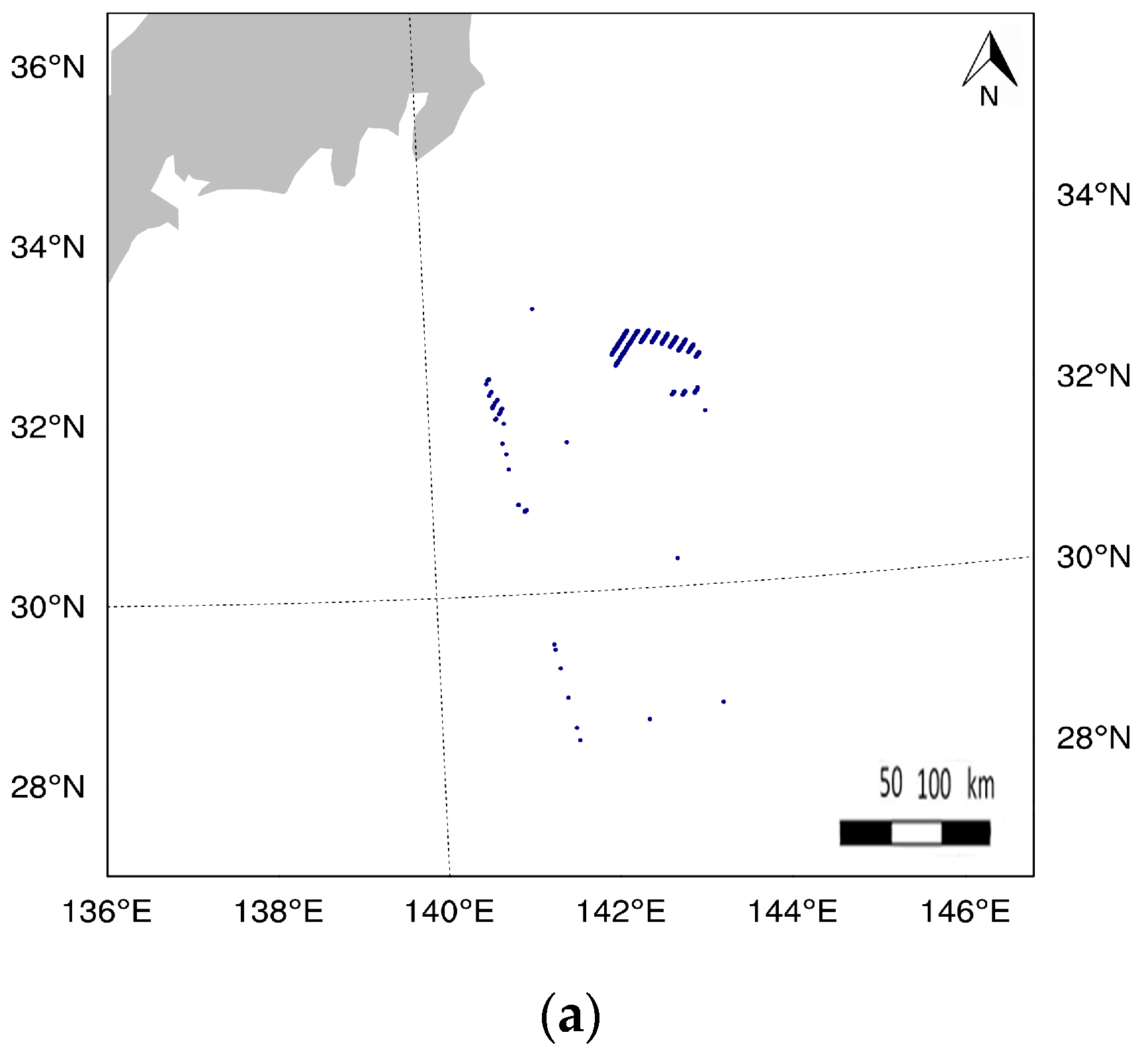
Three groups of experiments are designed to investigate the impact of SAR wind data in three-dimensional variational system for the Weather Research and Forecasting Model (WRF 3DVAR). These runs are referred to as the basic control experiment (CNTL) without observations, the SAR_uv experiment assimilating u and v, and the SAR_sd experiment assimilating the SAR wind speed and direct retrievals. The background fields were derived from a WRF simulation, which was integrated from 0000 UTC 28 August 2016 for 24 h, and the National Centers for Environmental Prediction (NCEP) final (FNL) analysis data was adopted in the WRF model. All the groups of experiments used the same background field. The analysis time for data assimilation was 0900 UTC 29 August 2016. In the SAR_uv and SAR_sd experiments, the assimilation window was 6 h, and the SAR observations were sounded at about 0830 UTC 29 August. After the assimilation, the analysis field was inputted to the WRF forecast model and run from the analysis time for 33 h. The input wind speed of the observations was checked to be less than 25 m/s and thinned to be 15 km. In both cases, 23,207 wind vectors were inputted. After quality control, only 327 wind vectors were accepted; 22,880 wind vectors were rejected in the SAR_sd case, and, in the SAR_uv case, 2896 wind components (u and v wind) were accepted and 20,311 wind vectors were rejected. The accepted observations for the two cases are plotted in Figure 3. The details of the three experiments are provided in Table 3.
3.3. Model Description
The WRF model developed by the United States National Centers for Environmental Prediction was used in this study, and the 3DVAR version 3.5 was used as the basic assimilation system for the SAR observations [29]. The UV operator and the SD operator were implemented in the 3DVAR system for the assimilation of the SAR UV wind and SD wind retrievals, respectively. The WRF 3.8 version was run as the forecast model.
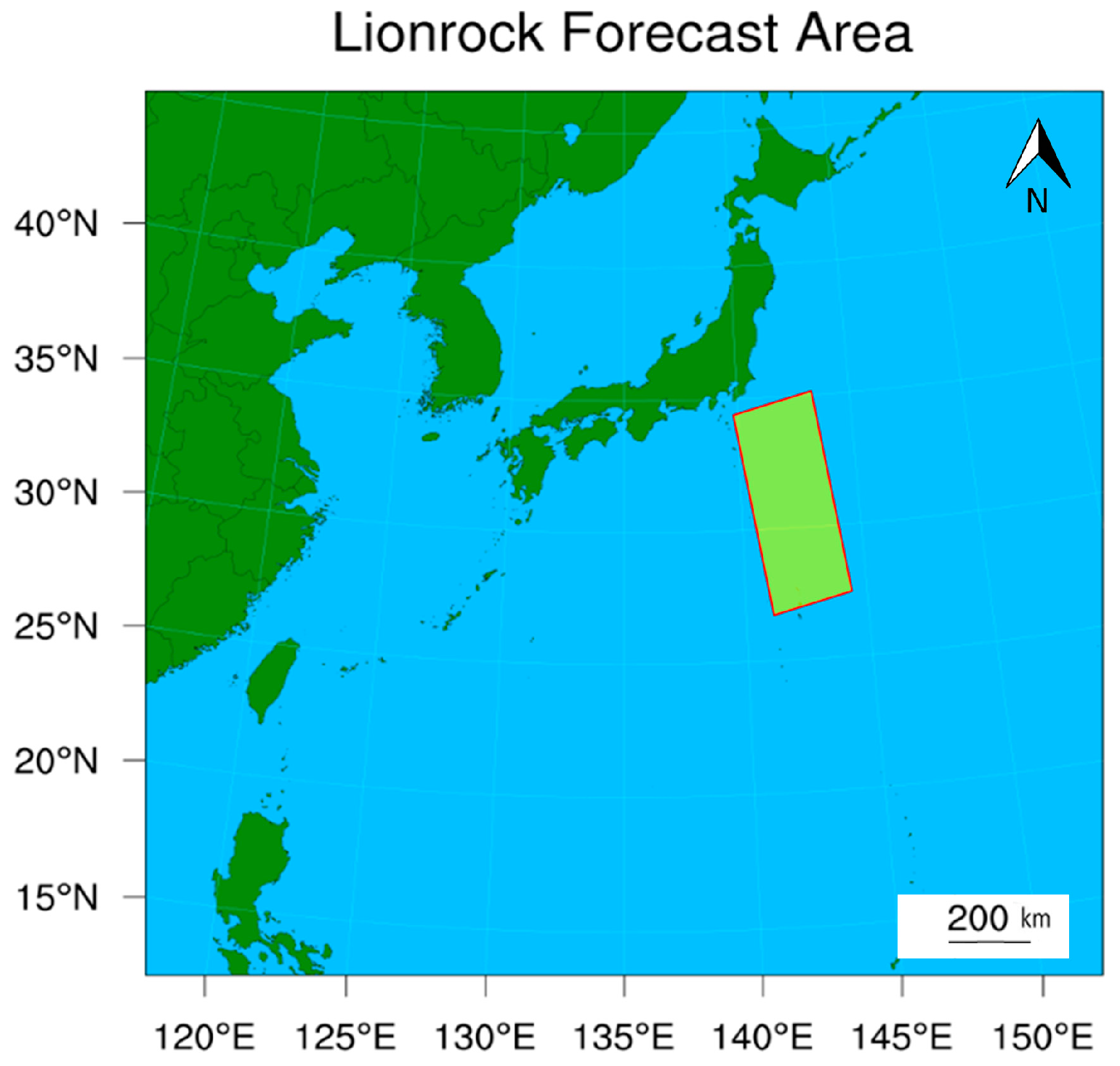
Various physical parameterization schemes are developed in the non-hydrostatic WRF model for the researchers to choose properly in order to simulate the atmospheric structures. The major physical options in our experiments include the WRF Single-Moment 3-class (WSM3) microphysics scheme [35], the Kain-Fritsch (KF) convective parameterization [36], and the Yonsei University (YSU) boundary layer scheme [37]. The domain of the WRF 3DVAR analysis and the WRF model simulation has 260 × 250 grid points, and the center of the domain is located at 30.0°N, 135°E (as shown in Figure 4). The horizontal resolution is 15km, and the vertical levels are 51 in the WRF model framework; the no-nesting method is utilized, and the Terrian-following coordinate (σ-coordinate) [38] at the top of the model atmosphere was located at 10 hPa. The SAR observed the area covering the center of the typhoon, and the structure of the wind field around the typhoon center can be seen clearly in Figure 1. Like the wind retrieval from the scatterometer observations, the SAR wind retrieval with speeds over 25 m/s also exhibits larger errors and is considered to be less reliable; the SAR wind retrieval with speeds less than 25 m/s is used in the assimilation.
4. Experimental Results
4.1. Wind Analysis at 10 m
To investigate the impact of the assimilation of SAR sea surface wind observations on the wind analysis at 10 m by the two different assimilation methods, the NCEP FNL data at 0900 UTC 29 August is used as the true wind field as the FNL data at the time of analysis time is of high accuracy [39].
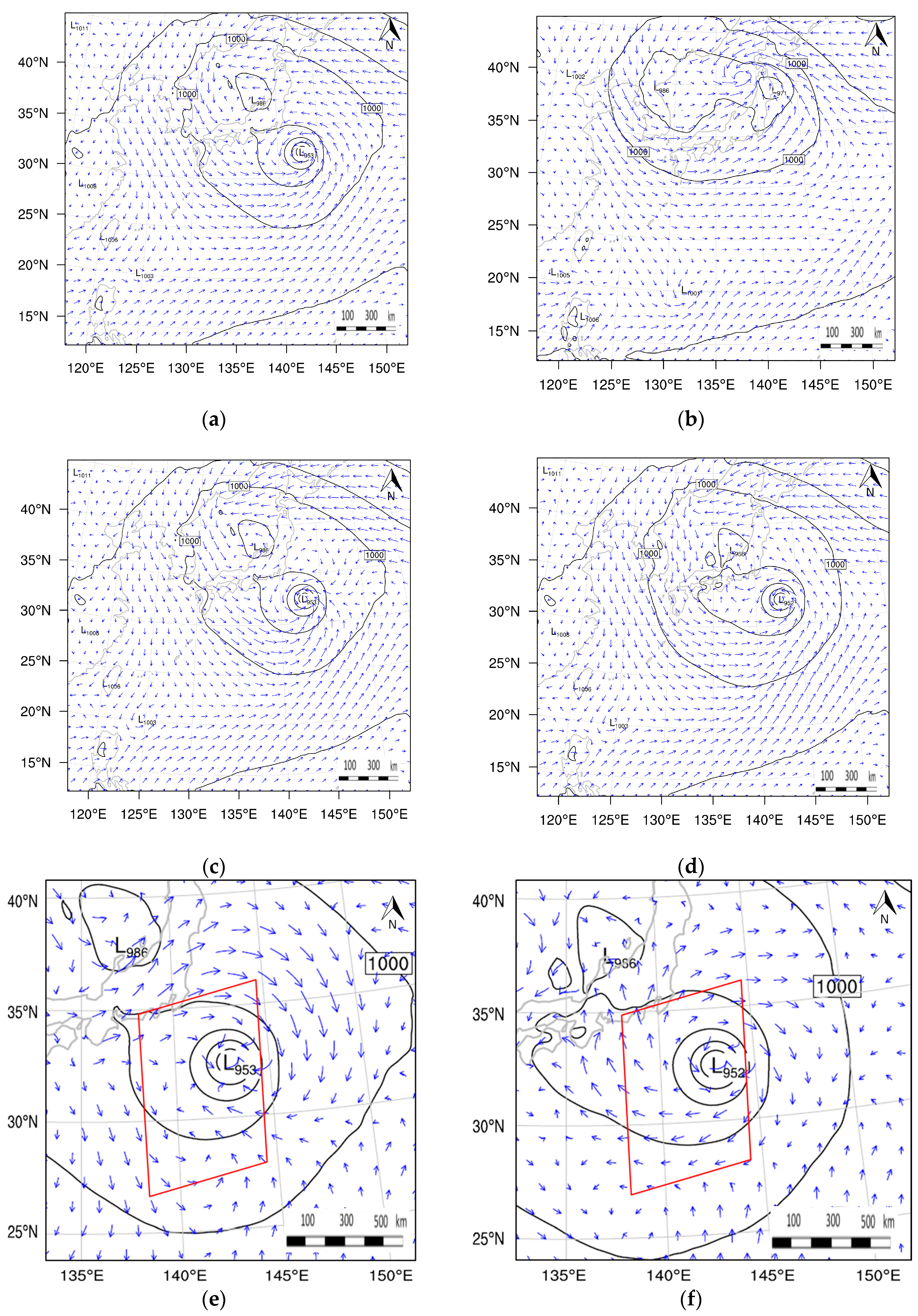
Figure 5 shows the wind fields at 10 m at 0900 UTC 29 August 2016. The Figure 5a,b, show the wind fields at 10 m from the NCEP FNL data and from the background field, respectively. The center of the typhoon in the FNL data is at 142°E, 32°N, while the typhoon center in the background is further north than the location in the FNL data. It can be seen from Figure 5a that the typhoon center of the real wind field is basically symmetrical and the wind field in the typhoon revolves around the typhoon center in the reverse clock direction. Compared with the real wind field, the center of the typhoon in the background field from Figure 5b is not obviously symmetrical. The direction of the wind field around the typhoon center is also counter-clockwise, but the strength simulation was significantly weaker than the real wind field. Moreover, the vortex structures and the pressure are very different in the two panels.
The Figure 5c,d, are the wind analysis at 10 m from the SAR_sd and SAR_uv, respectively. The tropical centers in both analysis fields are very close to the location in the FNL data. The wind fields from two analysis experiments are close to the real wind field. The wind field structure and the intensity of the typhoon in both assimilation analysis fields are basically consistent with those of the typhoon wind field. The observation data of the assimilated SAR can effectively adjust the background field and provide an accurate wind field at 10 m for the forecasting model. However, the pressure intensity in the typhoon center from the SAR_uv is slightly lower than that for the true field. The typhoon structure in the SAR_sd analysis is more symmetrical than the SAR_uv analysis. The spatial pressure distribution in SAR_sd is similar to the true wind field (Figure 5a), and the wind field in SAR_sd is also close to the true wind field. These results indicate that the analysis field from the SAR_sd experiment is closer to the FNL truth.
The Figure 5e,f are the analytical deviation at 10 m in the center of typhoon from the SAR_sd and the SAR_uv experiments, respectively. The red diamond region represents the area covered by the SAR observations. The analysis deviation is derived from the true field subtracted by the analysis. The smaller the analysis deviation, the more accurate the analysis field is. In the red frames, most of the arrows in Figure 5e are shorter than the arrows in Figure 5f; this indicates that the magnitude of the wind speed deviation of SAR_sd is smaller than that of SAR_uv. We can infer that the wind speed of the SAR_sd analysis is closer to the real wind speed; even the direction deviation is sometimes the same as the real wind field and sometimes contrary to the real wind field. A clockwise wind field orientation in Figure 5e,f indicates that the wind speed is underestimated, whereas a counter-clockwise wind field orientation indicates that the wind speed is overestimated. Almost all the wind direction of the deviation of SAR_uv is opposite to the real wind field, indicating that the wind speed is underestimated. However, comparing this with the observation bias outside the observation coverage area, it can be found that the impact of the analysis bias of SAR_sd is spread beyond the observation range and the deviation in both the left and right sides of the observation area is relatively large. The assimilation of SAR observations by the method to assimilate spd and dir can have a good influence in the observation area, and it may have some negative effects out of the periphery of the scanning area. This also can be seen in the northeastern side of the typhoon center on the right side of the SAR observation area in Figure 5c, where the wind speed and wind direction are significantly different from the real wind field. The impact of the analysis of SAR_uv is small both inside and outside of the periphery of the observation area, but it is not negative out of the periphery of the observed coverage area.
4.2. Analysis Bias at Different Height
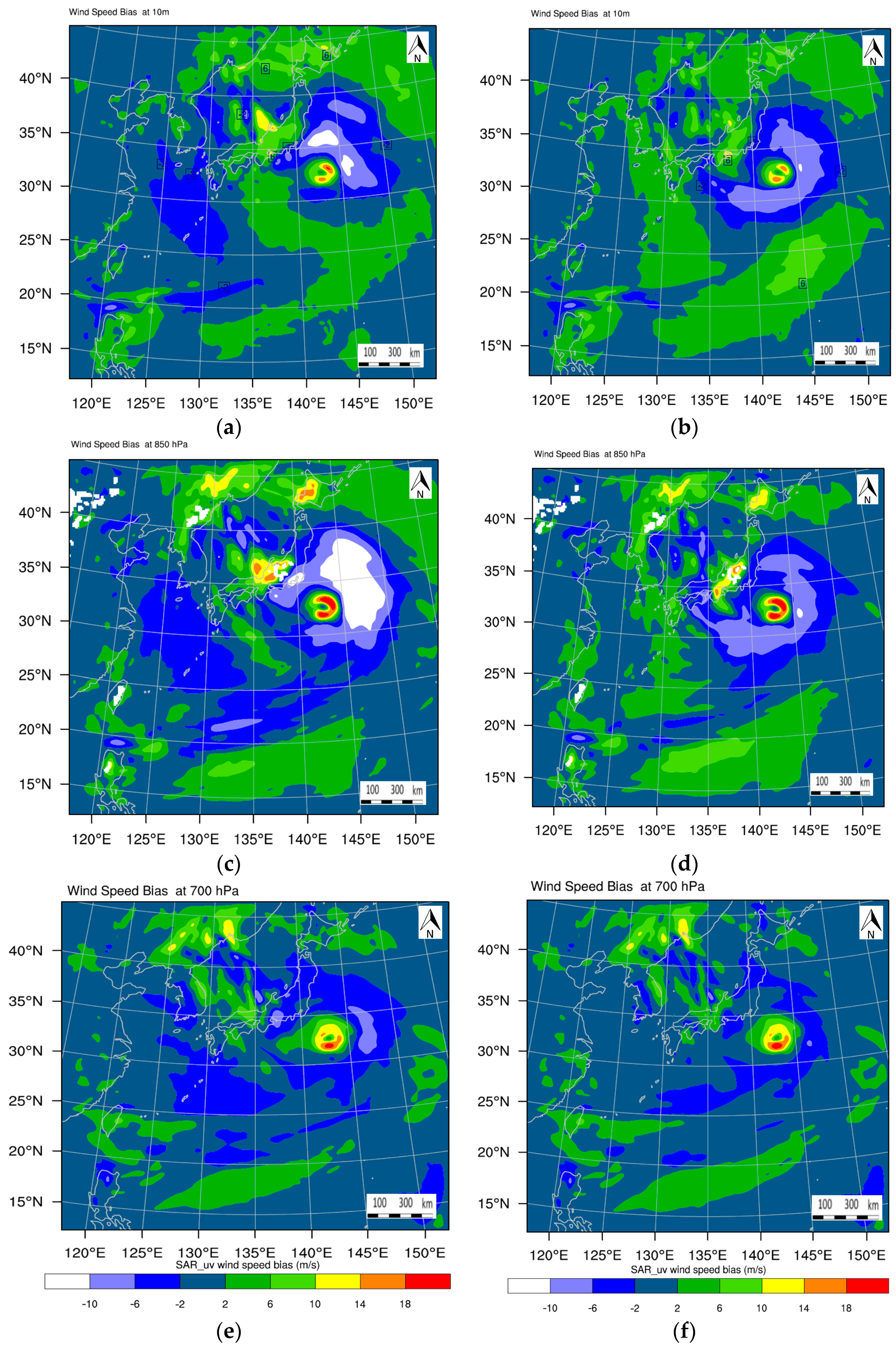
To assess the impact of the SAR sea surface wind observations on the analysis in of the vertical height of a typhoon, the analysis biases of wind speed for SAR_sd and SAR_uv at 10 m at 850 hPa, 700 hPa, 500 hPa, and 300 hPa are investigated. The analysis bias is derived from the true field subtracted by the analysis, and the NCEP FNL analysis at the analysis time is used as the true field.
The top two panels are the analysis bias of the wind speed at 10 m. There is an area of bias of −6 to −2 m/s in SAR_sd, and the area of bias is significant smaller than the area of SAR_uv out of the periphery of the TC. Generally the minimum bias of −2 to 2 m/sis the dominance area of the two panels, and this kind of area in SAR_sd is larger than in SAR_uv. These results indicate that the analysis by SAR_sd at 10 m is more accurate than that of SAR_uv. The middle two panels show the analysis bias of wind speed at 850 hPa. Figure 6c shows that, although there is an area of analysis bias of SAR_sd lower than −10 m/s in the northeast of the TC center, the bias is small in the southwest of the TC center, where many SAR sea surface wind observations exist. There is a large area of bias of −6 to −2 m/s in the west of the periphery of the TC from SAR_sd; this indicates that, in this area, the wind speed of SAR_sd is slower than the true wind field. Figure 6d shows there is a large area of analysis bias of −10 to −6 m/s just around the TC center from SAR_uv. There is a large area of analysis bias of 2 to 6 m/s in the periphery of the TC from SAR_uv, indicating that the wind speed is larger than the true wind field in this area for SAR_uv. Figure 6e,f show the analysis bias of wind speed at the 700 hPa for SAR_sd and SAR_uv, respectively. The two panels are similar, the main bias is −2 to 2 m/s, the lower bias is more from SAR_sd, and the higher bias is more from SAR_uv. The results at 500 hPa and 300 hPa are almost the same; the figures are not shown.
4.3. Analysis Increment for Different Analysis Parameters
The results described above show that the analysis of SAR_sd is closer to the NCEP FNL data; it is more accurate than the analysis of SAR_uv. We can investigate the analysis increment to derive some verification for the two types of SAR wind observations. The larger the analysis increment is, the more improvement brought by the observations, as both assimilation experiments were based on the same background and literal boundary conditions.
Figure 7 presents the average root mean square error (RMSE) of the analysis increment for both the SAR_sd and SAR_uv experiments. The analysis of u wind, v wind, temperature, and relative humidity is described in Figure 7a–d, respectively. The results from Figure 7a,b are almost the same. It can be seen that the SAR wind observations improved u and v analysis mainly from the surface to 450 hPa. Above 450 hPa, the analysis increment is nearly 0 and the information on u and v comes from the background. For the analysis of both u and v, the RMSE increment of the two experiments reached the maximum at 950 hPa. For the Figure 7c,d, it can be seen that the analysis increment exists in the whole vertical layer for both temperature and relative humidity. The maximum RMSE exists between 850 hPa and 800 hPa, and the RMSE of temperature is smaller than that of relative humidity. Generally, from the four panels, the results show that the RMSE from SAR_sd is larger than the RMSE from SAR_uv; this indicates the assimilation of spd and dir has larger improvement than the assimilation of u and v for the same SAR sea surface wind.
4.4. Forecast Results
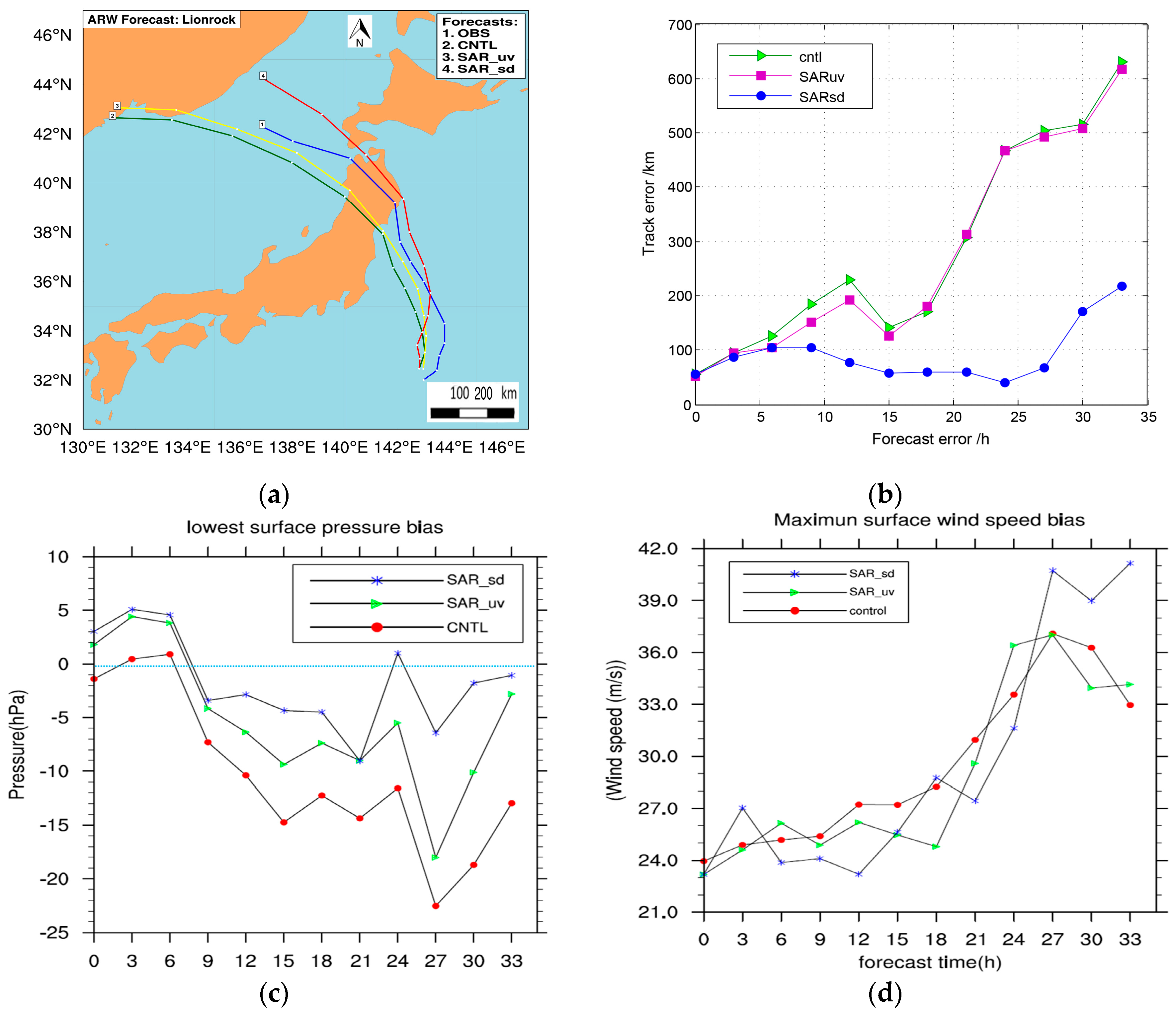
To verify how the assimilation of SAR sea surface wind affects the TC forecasts, the forecast skills of the track, the track error, the minimum sea level pressure (MSLP) error, and the absolute maximum wind speed error were assessed by comparing the forecasts from the SAR_sd and SAR_uv experiments with the CNTL experiment in Figure 8. The ‘best track’, minimum sea level pressure, and absolute maximum wind speed data for Typhoon Lionrock are obtained from the China Meteorological Administration (CMA).
Figure 8a shows the 33 h track forecasts of Lionrock initialized at 0900 UTC 29 August 2016. The best track positions from CMA are the blue line. The forecast tracks from the two SAR observation experiments agree better with the best track than that of the CNTL experiment, especially the track forecast from SAR_sd experiment after the 9 h forecast. The SAR sea surface wind prevented the track forecast from moving clearly westward too fast, even though SAR_sd moved westward in the first 9 h. All the predicted tracks moved faster than the best track. Generally, the track forecast from SAR_sd was closer to the best track than the track forecast from SAR_uv, and the landfall position in Japan from SAR_sd was closest to the position from the best track.
Mean absolute track error, MSLP error, and mini and absolute maximum wind speed error as a function of forecast range for Lionrock are shown in Figure 8b–d. We found that the track errors of SAR_uv and CNTL are almost the same, and they consistently increase, excepting the 15 h and 18 h forecast. The track error of SAR_sd is smaller those that of SAR_uv and CNTL, excepting the first 3 h, and is basically within 100km. The time after the 24 h forecast is the landing time for Lionrock; the track error from SAR_sd is about 45 km and is the smallest in the whole forecast time. The positive impact on the track forecast lasted for 27 h in SAR_sd, but the track error increases after 27 h. The MSLP error from SAR_sd is almost less than 5hPa for the whole forecast time, excepting the time after the 21 h forecast, and reached the minimum after the 9 h forecast even though it is the largest in the first 9 h compared with CNTL and SAR_uv. The maximum wind speed bias of SAR_sd is smaller than that of SAR_uv and CNTL during the forecast time 5~15 h and 20~25h. However, the bias from all three experiments is larger than 22 m/s, which may be related to the lack of perfection of the model itself [40].
5. Discussion and Conclusions
This study investigates the impact of SAR sea surface wind observations assimilated in the WRFDA system under typhoon conditions. The method to assimilate the wind speed (spd) and the direction (dir) was implemented in the WRFDA system and was compared with the conventional method, which assimilates the u and v wind components. The sea surface wind observations from the satellite-derived C-band Sentinel-1SAR were assimilated, and observational errors in the quality control were discussed for the two forms of wind state vectors. NCEP FNL analysis and reanalysis data distributed by the CMA were used to test and validate both assimilation methods.
Compared with the CNTL experiment, only the SAR sea surface wind observations in the center of the typhoon were assimilated in this study, but the results show that the SAR wind observations improved the analysis of Typhoon Lionrock in terms of the whole vertical height, and the improvement is significant below the height of 450 hPa, especially near 850 hPa, where the maximum improvement was reached. The assimilation of the SAR sea surface wind not only improved the analysis of wind but also improved the analysis of temperature and relative humidity. The SAR sea surface wind observations with a high resolution improved the depiction of the dynamic and thermodynamic vortex structure, especially by the method of the assimilation of spd and dir, which resulted in a reasonable observational error of dir, rather than the method of the assimilation of u and v wind without the consideration of the impact of dir. In the experiments, SAR_sd brought the TC environment fields closer to the NCEP FNL and observations and produced better analyses and forecasts for Typhoon Lionrock, compared with SAR_uv, using the same background and lateral boundary.
In this study, the SAR sea surface observations increase the number of effective observations in the typhoon area. However, many observations were still excluded after the thinning of the observations. This is because NWP systems run at low spatial resolutions, which is typically at 10 to 50 km resolution, and the high-resolution SAR data should be thinned to be compatible with the data assimilation system. The next generation data assimilation system with high resolution designed for limited area models could benefit from assimilating nearly full-resolution SAR data and could improve the typhoon forecast.
The strict QC_co method was applied for both kinds of assimilation methods to assimilate more accurate observations. The QC_co method was applied to the methods of assimilating u and v wind, but many wind vectors like the OBS4 in Figure 2 were still accepted after the quality control, and these observations may reduce the impact of the analysis. In addition, dir was derived independently from spd for satellite-derived SAR sea surface wind observations. It is likely that the QC_co method is too strict for the method of assimilating spd and dir to accept the most useful observations. For example, in the Typhoon Lionrock case, the wind vectors with huge but appropriate spd were rejected because the dir could not pass the quality control. The wind speed and wind direction are separately derived from SAR observations, and their errors are independent. Thus QC_al could be suitable for the method of assimilating spd and dir, and larger thresholds with more than five times the innovation could be applied for the wind dir for this procedure. Further investigation of the quality control schemes for SAR-derived winds should be studied in the future. The numerical forecast results for this case show better results for the SAR_sd method than for the SAR_uv method. The SAR_sd method looks very promising for wind assimilation under typhoon conditions, but more cases need to be considered to draw final conclusions.
Acknowledgments
The authors acknowledge the support of the National Natural Science Foundation (41605070) and the Key Research and Development Program of Hainan Province (ZDYF2017167).
Author Contributions
Yi Yu decided on the direction of the study with help from Xiaofeng Yang, implemented the code for comparison, and completed the writing and implementation of the co-authors’ comments. Xiaofeng Yang retrieved sea surface winds from the Sentinel-1 synthetic aperture radar (SAR). Weimin Zhang supported the method and the interpretation of the results with comments and discussions. Boheng Duan supported the implementation of the code for the data assimilation of wind speed and wind direction. Xiaoqun Cao and Hongze Leng provided guidance on the meteorological side of the method. All co-authors have participated in revising the draft from the first collection of ideas to the final version of the paper.
Conflicts of Interest
The authors declare no conflicts of interest.
References
- Zhang, Y.; Chen, Y.; Zhu, M. Research on ocean surface wind field retrievals from SAR. Electron. Meas. Technol. 2007, 30, 36–38. [Google Scholar]
- Dagestad, K.F.; Horstmann, J.; Mouche, A.; Perrie, W.; Shen, H.; Zhang, B.; Li, X.; Monaldo, F.; Pichel, W.; Lehner, S.; et al. Wind retrieval from synthetic aperture radar-an overview. In Proceedings of the 4th SAR Oceanography Workshop (SEASAR 2012), Tromsø, Norway, 18–22 June 2012. [Google Scholar]
- Chang, R.; Zhu, R.; Badger, M.; Hasager, C.B.; Xing, X. Offshore wind resources assessment from multiple satellite data and WRF modeling over South China Sea. Remote Sens. 2015, 7, 467–487. [Google Scholar] [CrossRef]
- Hasager, C.; Badger, M.; Peña, A.; Larsén, X.; Bingöl, F. SAR-based wind resource statistics in the Baltic Sea. Remote Sens. 2011, 3, 117–144. [Google Scholar] [CrossRef] [Green Version]
- Yu, Y.; Zhang, W.; Wu, Z.; Yang, X.; Cao, X.; Zhu, M. Assimilation of HY-2A scatterometer sea surface wind data in a 3DVAR data assimilation system—A case study of Typhoon Bolaven. Front. Earth Sci. 2015, 92, 192–201. [Google Scholar] [CrossRef]
- Yang, X.; Li, X.; Zheng, Q.; Gu, X.; Pichel, W.G.; Li, Z. Comparison of Ocean-Surface Winds Retrieved From QuikSCAT Scatterometer and Radarsat-1 SAR in Offshore Waters of the U.S. West Coast. IEEE Geosci. Remote Sens. Lett. 2011, 8, 163–167. [Google Scholar] [CrossRef]
- Danielson, R.; Dowd, M.; Ritchie, H. Marine Wind Analysis with the Benefit of Radarsat-1 Synthetic Aperture. In Proceedings of the OceanSAR 2006—Third Workshop on Coastal and Marine Applications of SAR, St. John’s, NL, Canada, 23–25 October 2006. [Google Scholar]
- Geldsetzer, T.; Pogson, L.; Scott, A.; Buehner, M.; Carrieres, T.; Ross, M.; Caya, A. Retrieval of sea ice and open water from SAR imagery for data assimilation. In Proceedings of the 7th IICWG Workshop on Sea Ice Data Assimilation and Verification, Frascati, Italy, 5–7 April 2016. [Google Scholar]
- Lin, H.; Xu, Q.; Zheng, Q. An overview on SAR measurements of sea surface wind. Proc. Nat. Sci. 2008, 18, 913–919. [Google Scholar] [CrossRef]
- Li, X.; Zhang, J.A.; Yang, X.; Pichel, W.G.; DeMaria, M.; Long, D.; Li, Z. Tropical cyclone morphology from spaceborne synthetic aperture radar. Bull. Am. Meteorol. Soc. 2013, 94, 215–230. [Google Scholar] [CrossRef]
- Perrie, W.; Zhang, W.; Bourassa, M.; Shen, H.; Vachon, P.W. Impact of satellite winds on marine wind simulations. Weather Forecast. 2008, 23, 290–303. [Google Scholar] [CrossRef]
- Yang, X.; Li, X.; Pichel, W.G.; Li, Z. Comparison of ocean surface winds from ENVISAT ASAR, MetOp ASCAT scatterometer, buoy measurements, and NOGAPS model. IEEE Trans. Geosci. Remote Sens. 2011, 49, 4743–4750. [Google Scholar] [CrossRef]
- Ahsbahs, T.; Badger, M.; Karagali, I.; Larsén, X. Validation of Sentinel-1A SAR Coastal Wind Speeds against Scanning LiDAR. Remote Sens. 2017, 9, 552. [Google Scholar] [CrossRef]
- Danielson, R.; Fillion, L.; Ritchie, H.; Dowd, M. Assimilation of SAR Wind Information IN Environment Canada’s High Resolution 3D-Var Analysis System. In Proceedings of the Third International Workshop, Frascati, Italy, 25–29 January 2010. [Google Scholar]
- Perrie, W.; Zhang, W.; Bourassa, M.; Shen, H.; Vachon, P.W. SAR-derived Winds from Hurricanes: Assimilative Blending with Weather Forecast Winds. In Proceedings of the Proceedings Ocean SAR 2006, St. John’s, NL, Canada, 1–3 October, 2006. [Google Scholar]
- Choisnard, J.; Laroche, S. Properties of variational data assimilation for synthetic aperture radar wind retrieval. J. Geophys. Res. 2008, 113, C050061-13. [Google Scholar] [CrossRef]
- Barker, D.; Huang, X.Y.; Liu, Z.; Auligné, T.; Zhang, X.; Rugg, S.; Ajjaji, R.; Bourgeois, A.; Bray, J.; Chen, Y.; et al. The weather research and forecasting model’s community variational/ensemble data assimilation system: WRFDA. Bull. Am. Meteorol. Soc. 2012, 93, 831–843. [Google Scholar] [CrossRef]
- Huang, X.Y.; Gao, F.; Jacobs, N.A.; Wang, H. Assimilation of wind speed and direction observations: A new formulation and results from idealized experiments. Tellus A 2013, 65, 19936. [Google Scholar] [CrossRef]
- Gao, F.; Huang, X.Y.; Jacobs, N.A.; Wang, H. Assimilation of wind speed and direction observations: Results from real observation experiments. Tellus A 2015, 67, 27132. [Google Scholar] [CrossRef]
- Li, X. The first Sentinel-1 SAR image of a typhoon. Acta Oceanol. Sin. 2015, 34, 1–2. [Google Scholar] [CrossRef]
- Friedman, K.; Li, X. Storm patterns over the ocean with wide swath SAR. Johns. Hopkins Univ. Appl. Phys. Lab. APL Tech. Dig. 2000, 21, 80–85. [Google Scholar]
- Li, X.; Pichel, W.G.; He, M.; Wu, S.Y.; Friedman, K.S.; Clemente-Colón, P.; Zhao, C. Observation of hurricane-generated ocean swell refraction at the Gulf Stream north wall with the RADARSAT-1 synthetic aperture radar. IEEE Trans. Geosci. Remote Sens. 2002, 40, 2131–2142. [Google Scholar]
- Zhang, G.; Li, X.; Perrie, W.; Hwang, P.A.; Zhang, B.; Yang, X. A Hurricane Wind Speed Retrieval Model for C-Band RADARSAT-2 Cross-Polarization ScanSAR Images. IEEE Trans. Geosci. Remote Sens. 2017, 55, 4766–4774. [Google Scholar] [CrossRef]
- Hersbach, H.; Stoffelen, A.; De Haan, S. An improved C-band scatterometer ocean geophysical model function: CMOD5. J. Geophys. Res. 2007, 112, C030061-18. [Google Scholar] [CrossRef]
- Du, Y.; Vachon, P.W. Characterization of hurricane eyes in RADARSAT-1 images with wavelet analysis. Can. J. Remote Sens. 2003, 29, 491–498. [Google Scholar] [CrossRef]
- Zhou, X.; Yang, X.; Li, Z.; Yu, Y.; Bi, H.; Ma, S.; Li, X. Estimation of tropical cyclone parameters and wind fields from SAR images. Sci. China Earth Sci. 2013, 56, 1977–1987. [Google Scholar] [CrossRef]
- Le Dimet, F.X.; Talagrand, O. Variational algorithms for analysis and assimilation of meteorological observations: Theoretical aspects. Tellus A 1986, 38, 97–110. [Google Scholar] [CrossRef]
- Zou, X.; Navon, I.M.; Sela, J. Control of gravitational oscillations in variational data assimilation. Mon. Weather Rev. 1993, 121, 272–289. [Google Scholar] [CrossRef]
- Barker, D.M.; Huang, W.; Guo, Y.R.; Bourgeois, A.J.; Xiao, Q.N. A three-dimensional variational data assimilation system for MM5: Implementation and initial results. Mon. Weather Rev. 2004, 132, 897–914. [Google Scholar] [CrossRef]
- Huang, X.Y.; Xiao, Q.; Barker, D.M.; Zhang, X.; Michalakes, J.; Huang, W.; Henderson, T.; Bray, J.; Chen, Y.; Ma, Z.; et al. Four-dimensional variational data assimilation for WRF: Formulation and preliminary results. Mon. Weather Rev. 2009, 137, 299–314. [Google Scholar] [CrossRef]
- Velden, C.S.; Hayden, C.M.; Paul Menzel, W.; Franklin, J.L.; Lynch, J.S. The impact of satellite-derived winds on numerical hurricane track forecasting. Weather Forecast. 1992, 7, 107–118. [Google Scholar] [CrossRef]
- Holmlund, K.; Velden, C.S.; Rohn, M. Enhanced automated quality control applied to high-density satellite-derived winds. Mon. Weather Rev. 2001, 129, 517–529. [Google Scholar] [CrossRef]
- Hollingsworth, A.; Lönnberg, P. The statistical structure of short-range forecast errors as determined from radiosonde data. Part I: The wind field. Tellus A 1986, 38, 111–136. [Google Scholar] [CrossRef]
- Raymond, T. Report on TC’s Key Activities and Main Events in the Region 2016. In Proceedings of the 49 Session ESCAP/WMO Typhoon Committee, Yokohama, Japan, 21–24 February, 2017. [Google Scholar]
- Hong, S.Y.; Dudhia, J.; Chen, S.H. A revised approach to ice microphysical processes for the bulk parameterization of clouds and precipitation. Mon. Weather Rev. 2004, 132, 103–120. [Google Scholar] [CrossRef]
- Kain, J.S. The Kain–Fritsch convective parameterization: An update. J. Appl. Meteorol. 2004, 43, 170–181. [Google Scholar] [CrossRef]
- Shin, H.H.; Hong, S.Y. Intercomparison of planetary boundary-layer parametrizations in the WRF model for a single day from CASES-99. Bound. Layer Meteorol. 2011, 139, 261–281. [Google Scholar] [CrossRef]
- Skamarock, W.C.; Klemp, J.B.; Dudhia, J. Prototypes for the WRF (Weather Research and Forecasting) model. Preprints. In Proceedings of the Ninth Conference Mesoscale Processes, American Meteorological Society, Fort Lauderdale, FL, USA, 11–15 July 2001. [Google Scholar]
- Mejia, J.F.; Murillo, J.; Galvez, J.M.; Douglas, M.W. Accuracy of the NCAR global tropospheric analysis (FNL) over Central South America based upon upper air observations collected during the SALLJEX. In Proceedings of the 8th International Conference on Southern Hemisphere Meteorology and Oceanography (ICSHMO), Foz do Iguaçu, Brazil, 24–28 April 2006. [Google Scholar]
- Xu, D.; Liu, Z.; Huang, X.Y.; Min, J.; Wang, H. Impact of assimilating IASI radiance observations on forecasts of two tropical cyclones. Meteorol. Atmos. Phys. 2013, 122, 1–18. [Google Scholar] [CrossRef]
Figure 1.
Windfield retrieved from Sentinel-1A synthetic aperture radar (SAR) Extra-wide Swath Mode data on 29 August 2016 at 08:32 UTC. (A) Sea surface radar backscattering map; (B) the SAR derived sea surface wind map.
Figure 1.
Windfield retrieved from Sentinel-1A synthetic aperture radar (SAR) Extra-wide Swath Mode data on 29 August 2016 at 08:32 UTC. (A) Sea surface radar backscattering map; (B) the SAR derived sea surface wind map.

Figure 2.
Diagram of background wind vector BKG and the observation wind vectors (OBS1, OBS2, OBS3, and OBS4) used to present the difference between thequality control procedures, QC_co and QC_al, of SAR_uv (standard assimilation method in theWeather Research and Forecasting Model Data Assimilation system (WRFDA), assimilating SAR wind observation in the form of u and v components) and SAR_sd (new assimilated method, assimilating SAR wind observation in the forms of wind speed and direction).
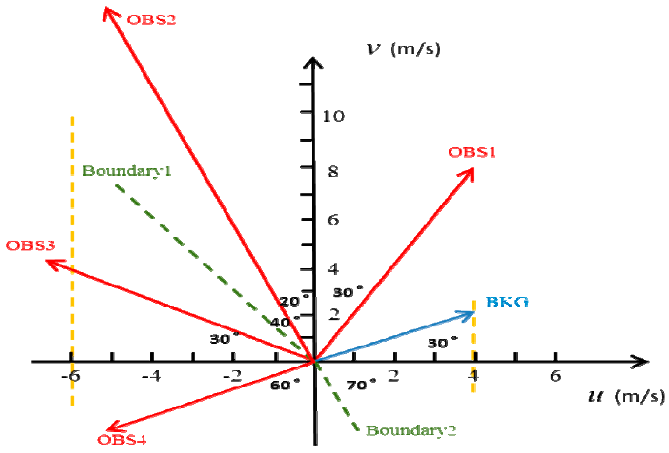
Figure 3.
The accepted observtion wind vectors in the (a) SAR_sd and in the (b) SAR_uv experiments. The blue points are the wind vectors.
Figure 3.
The accepted observtion wind vectors in the (a) SAR_sd and in the (b) SAR_uv experiments. The blue points are the wind vectors.

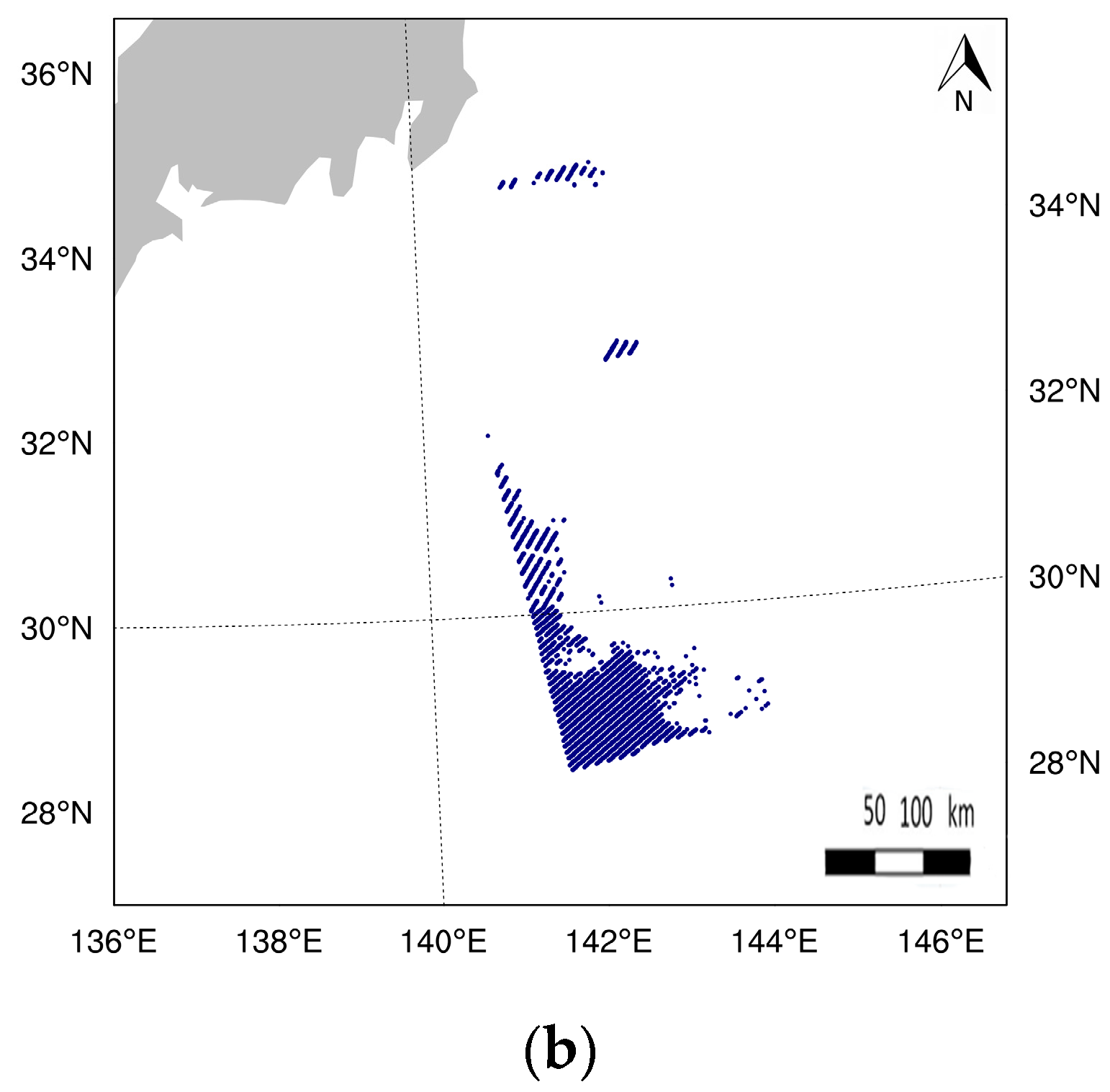
Figure 4.
The domain area for theWeather Research and Forecasting (WRF) model simulation.The corverage of SAR observations is shownin the red frame.
Figure 4.
The domain area for theWeather Research and Forecasting (WRF) model simulation.The corverage of SAR observations is shownin the red frame.

Figure 5.
The 10m wind field at 0900 UTC 29 August 2016 from (a) the NCEP FNL data in (b) the background field; the wind analysis field at 10m from (c) SAR_sd and (d) SAR_uv. The bottom two panelsare the analysis bias derived from the analysis subtracting the FNL data for (e) SAR_sd and (f) SAR_uv. The red frames mark the area of the SAR wind observations. Note the different spatial scales of (e,f) as compared to (a–d).

Figure 6.
The analysis bias the SAR_sd (left panels) and the SAR_uv (right panels) at (a,b) 10 m at (c,d) 850 hPa, and at (e,f) 700 hPa.
Figure 6.
The analysis bias the SAR_sd (left panels) and the SAR_uv (right panels) at (a,b) 10 m at (c,d) 850 hPa, and at (e,f) 700 hPa.

Figure 7.
Root mean square error (RMSE) profiles of the analysis increments from the SAR_sd experiment (round point) and the SAR_uv experiment (triagle piont) for (a) u wind, (b) v wind, (c) temperature, and (d) relatively humidity.
Figure 7.
Root mean square error (RMSE) profiles of the analysis increments from the SAR_sd experiment (round point) and the SAR_uv experiment (triagle piont) for (a) u wind, (b) v wind, (c) temperature, and (d) relatively humidity.
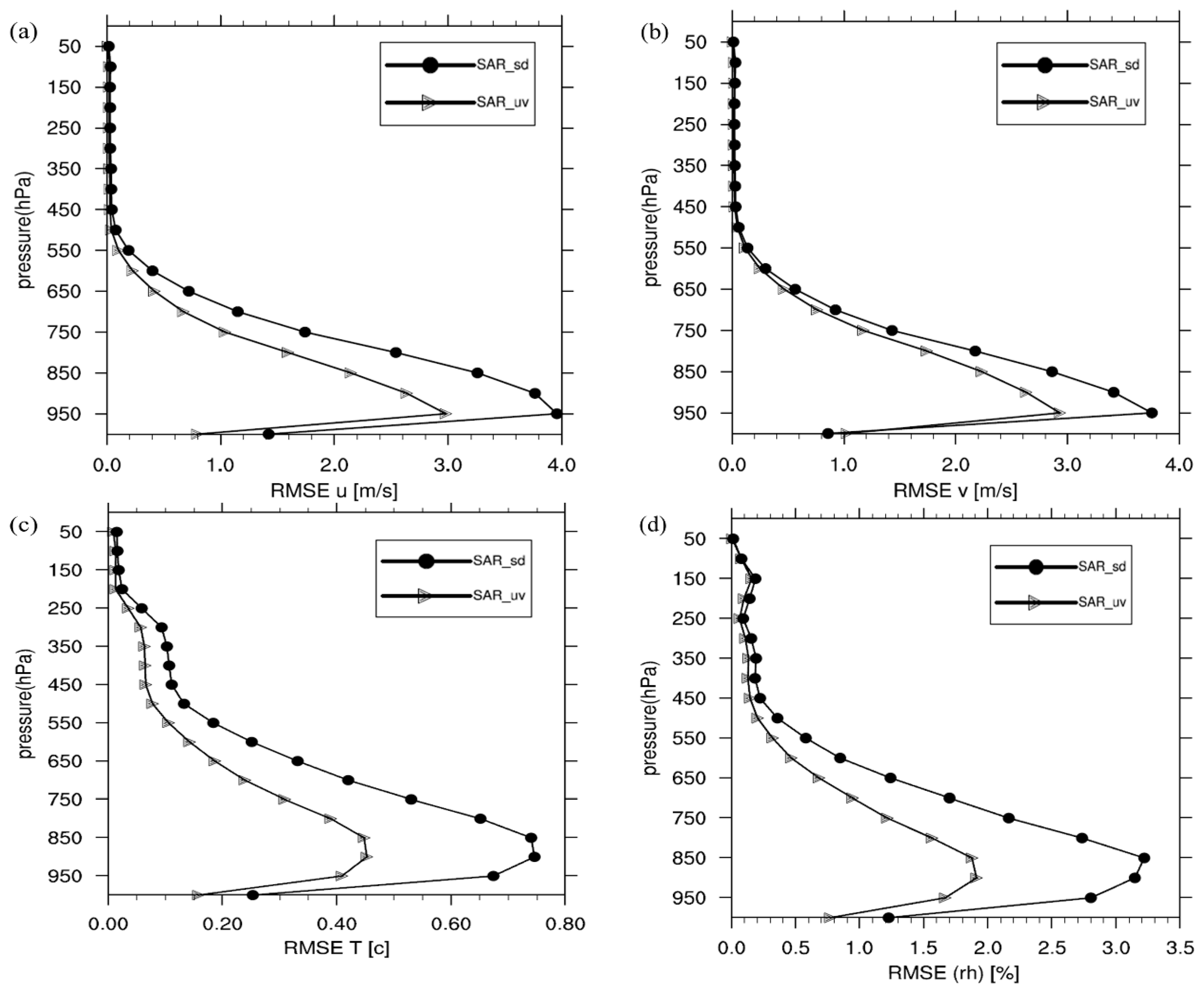
Figure 8.
For Typhoon Lionrock: (a) 33h track forecast initialized at 0900 UTC August 2016; (b) mean absolute track errors; (c) mean absolute maximum wind speed errors; (d) minimum sea level pressure as a function of forecast lead time.
Figure 8.
For Typhoon Lionrock: (a) 33h track forecast initialized at 0900 UTC August 2016; (b) mean absolute track errors; (c) mean absolute maximum wind speed errors; (d) minimum sea level pressure as a function of forecast lead time.


Table 1.
The detail value of the background and four kinds of observations.
| Wind Vectors | Spd (m/s) | Dir (°) | U (m/s) | V (m/s) |
|---|---|---|---|---|
| BKG | 4.61 | 30 | 4.00 | 2.31 |
| OBS1 | 8.00 | 60 | 4.00 | 6.93 |
| OBS2 | 14.62 | 110 | −4.99 | 13.74 |
| OBS3 | 6.80 | 150 | −5.89 | 3.40 |
| OBS4 | 5.60 | 210 | −4.85 | −2.80 |
Table 2.
The remaining components after quality control for the two assimilation methods.
| Observation Types | SAR_sd | SAR_uv | ||
|---|---|---|---|---|
| QC_co | QC_al | QC_co | QC_al | |
| OBS1 | spd, dir | spd, dir | u, v | u, v |
| OBS2 | - | dir | - | u |
| OBS3 | - | spd | - | v |
| OBS4 | - | spd | u, v | u, v |
Table 3.
Details of the three experiments.
| Experiment | Data | Operator | Quanlity Controll | Accept Obs. | Reject Obs. |
|---|---|---|---|---|---|
| CNTL | - | - | - | - | - |
| SAR_uv | u and v componets | UV operator | QC_co | 2896 | 20,311 |
| SAR_sd | spd and dir | SD operator | QC_co | 327 | 22,880 |
© 2017 by the authors. Licensee MDPI, Basel, Switzerland. This article is an open access article distributed under the terms and conditions of the Creative Commons Attribution (CC BY) license (http://creativecommons.org/licenses/by/4.0/).
Share and Cite
MDPI and ACS Style
Yu, Y.; Yang, X.; Zhang, W.; Duan, B.; Cao, X.; Leng, H. Assimilation of Sentinel-1 Derived Sea Surface Winds for Typhoon Forecasting. Remote Sens. 2017, 9, 845. https://doi.org/10.3390/rs9080845
AMA Style
Yu Y, Yang X, Zhang W, Duan B, Cao X, Leng H. Assimilation of Sentinel-1 Derived Sea Surface Winds for Typhoon Forecasting. Remote Sensing. 2017; 9(8):845. https://doi.org/10.3390/rs9080845
Chicago/Turabian StyleYu, Yi, Xiaofeng Yang, Weimin Zhang, Boheng Duan, Xiaoqun Cao, and Hongze Leng. 2017. "Assimilation of Sentinel-1 Derived Sea Surface Winds for Typhoon Forecasting" Remote Sensing 9, no. 8: 845. https://doi.org/10.3390/rs9080845
Note that from the first issue of 2016, this journal uses article numbers instead of page numbers. See further details here.