Article

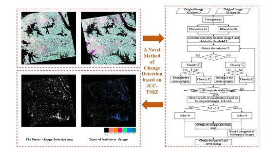
A Novel Method of Change Detection in Bi-Temporal PolSAR Data Using a Joint-Classification Classifier Based on a Similarity Measure

1
State Key Laboratory of Information Engineering in Surveying, Mapping and Remote Sensing, Wuhan University, Wuhan 430079, China
2
Huffington Department of Earth Sciences, Southern Methodist University, Dallas, TX 75275, USA
*
Author to whom correspondence should be addressed.
Remote Sens. 2017, 9(8), 846; https://doi.org/10.3390/rs9080846
Submission received: 29 May 2017 / Revised: 4 August 2017 / Accepted: 9 August 2017 / Published: 15 August 2017

Abstract

:
Accurate and timely change detection of the Earth’s surface features is extremely important for understanding the relationships and interactions between people and natural phenomena. Owing to the all-weather response capability, polarimetric synthetic aperture radar (PolSAR) has become a key tool for change detection. Change detection includes both unsupervised and supervised methods. Unsupervised change detection is simple and effective, but cannot detect the type of land cover change. Supervised change detection can detect the type of land cover change, but is easily affected and depended by the human interventions. To solve these problems, a novel method of change detection using a joint-classification classifier (JCC) based on a similarity measure is introduced. The similarity measure is obtained by a test statistic and the Kittler and Illingworth (TSKI) minimum-error thresholding algorithm, which is used to automatically control the JCC. The efficiency of the proposed method is demonstrated by the use of bi-temporal PolSAR images acquired by RADARSAT-2 over Wuhan, China. The experimental results show that the proposed method can identify the different types of land cover change and can reduce both the false detection rate and false alarm rate in the change detection.

Graphical Abstract

1. Introduction

In remote sensing, change detection is the process of identifying the changes that have occurred on the Earth’s surface by multi-temporal images acquired in the same geographical area at different times [1,2]. As a result of the repeat-pass nature of satellite orbits, time series of remote sensing images can be acquired to perform change detection. In recent years, optical sensors and synthetic aperture radar (SAR) have been widely used for change detection, in applications such as land-use and land cover dynamic analysis [3,4], environmental monitoring [5,6,7,8,9], etc.
On the one hand, optical images have been widely applied in change detection [2,3,10,11]. Unfortunately, night-time and severe weather often limit the use of optical images in practice [12]. On the other hand, thanks to the unique characteristics of microwaves, SAR sensors can not only acquire periodic images regardless of weather and time, but can also provide valuable information on biophysical and geophysical parameters [13,14,15,16]. Although a number of methods have been proposed for single-channel SAR images [17,18,19,20], the interpretation of the backscattering changes of the land cover is limited [7]. When compared with single-channel SAR images, polarimetric synthetic aperture radar (PolSAR) images contain both phase and amplitude information from the radar returns transmitted in two different polarizations, and use more scattering information [21]. The current methods of change detection based on SAR images can be divided into two categories: unsupervised approaches and supervised approaches.
Because of the simple design, unsupervised change detection represents a hot research field in the change detection. In general, unsupervised change detection in SAR images involves: (1) preprocessing; (2) generating the comparison image; and (3) choosing an optimal threshold to divide comparison images into changed and unchanged parts. The preprocessing of multi-temporal SAR images mainly involves radiometric calibration, speckle filtering [22,23], and image co-registration, which are all critical to change detection. The pixel values of SAR images are directly related to the radar backscatter of the scene after radiometric calibration. This condition is necessary for the comparison of SAR images acquired at different dates. Speckle filtering is usually carried out to suppress the speckle before the change detection and classification of SAR images. Image co-registration in the preprocessing is aimed at reducing the errors caused by the misregistration of the images. It aligns the images used in the change detection as precisely as possible, so that corresponding pixels in the images correspond to the same position in the scene. In the second step, two preprocessed images of the same geographical area at different times are compared to generate the comparison image. There are many methods of generating the comparison image using two co-registered images, such as the ratio or log-ratio operator of SAR amplitudes or intensities [17,19,20], the hidden Markov chain model [24,25], the Kullback–Leibler divergence method [26], etc. These methods are usually applied in multi-temporal single-channel SAR-based change detection. Unlike the above methods, test statistics can be applied in not only single-channel SAR data, but also PolSAR data [5,27,28]. The use of multichannel data (coherency or covariance matrix) can obtain a more accurate comparison image. In the third step of change detection analysis, the change detection map can be obtained by the decision threshold of the comparison image. Several algorithms are widely used to automatically determine the threshold, such as the constant false alarm rate (CFAR) algorithm [29], Otsu’s thresholding method [30], Kapur’s entropy algorithm [31], the Kittler and Illingworth (K & I) algorithm [32], etc. Although unsupervised change detection approaches are relatively simple, straightforward, and easy to implement and interpret, they cannot determine the type of land cover change.
For another, as one of the typical supervised approaches, post-classification comparison (PCC) methods can provide information on both the change detection map and the type of land cover change. PCC involves performing change detection by comparing separate supervised classifications of images obtained on different dates [33]. The procedure of PCC includes the following steps: (1) preprocessing; (2) classification of the multi-temporal SAR images; and (3) comparing the independently produced classifications of step 2, and obtaining the change map and the map showing the type of land cover change [34]. The first step of preprocessing is the same as the unsupervised change detection above. In the second step, a classification method is used to obtain the classification results of the time-series images. Unsupervised classification cannot determine the class label; therefore, these methods are limited in PCC [35]. However, some supervised classification methods [36], such as the Wishart classifier based on maximum likelihood [37], support vector machine (SVM) [38,39], and random forests (RF) [12], are widely used with PolSAR images. In the third step, the results of the classification are used to obtain the change detection map and land cover change map. Although PCC can provide more information than the unsupervised methods of change detection, it is liable to be affected by the significant cumulative error caused by the single remote sensing image classification during the change detection.
Combining the respective advantages of the unsupervised and supervised methods of change detection, Han and Zhou [35] designed joint-classification classifier (JCC) change detection based on improved fuzzy adaptive resonance theory mapping in bi-temporal optical images, and obtained a better performance than PCC. However, this method is not suitable for bi-temporal SAR images. Li et al. [40] used a JCC method based on k-means for bi-temporal single-channel SAR image change detection. However, k-means is an unsupervised classifier, so the class labels need to be determined after classification; therefore, the algorithm has its limitations. The generalization of the methods based on JCC to bi-temporal SAR images has proved to be nontrivial. Moreover, literature on change detection based on JCC in bi-temporal PolSAR data is sparse.
To solve the above problems, the objective of this study is to develop a novel method for change detection using bi-temporal PolSAR images. The proposed method using JCC based on a similarity measure not only has the advantage of unsupervised change detection in detecting a similarity measure for each pixel, but also has the advantage of supervised change detection in obtaining the type of land cover change. The similarity measure map includes the calculating comparison image and threshold choosing. The variances of the bi-temporal images are used to decide the sequence of classification, and the similarity measure is used to automatically control the JCC. Test statistics based on maximum likelihood estimation (MLE) and the Kittler and Illingworth (K & I) algorithm [4] are used to obtain the similarity measure map of the same geographical area at different times. Furthermore, the similarity measure map can determine the similarity of the same region at different times, and can distinguish the similar parts and the different parts. The similar parts are considered as the same category, and the different parts are classified, respectively. The classifier in the proposed method is the complex Wishart classifier, which is suitable for PolSAR data [37,41]. After finishing the joint-classification classifier based on Test statistics and the Kittler and Illingworth (JCC-TSKI) procedure, we can obtain the binary change detection map (changed and unchanged) and the map of land cover change.
The remainder of this paper is organized as follows. Section 2 presents a brief introduction to the fundamental theory and details of the proposed change detection framework. Section 3 describes the experimental results. In Section 4, we draw our conclusions.

2. Materials and Methods

2.1. The Model of PolSAR Data

Assuming that a p-dimensional random complex vector Q = [ q 1 , q 2 , . q p ] T follows a complex multi-variate normal distribution with mean 0 and dispersion matrix Σ Q = E [ Q Q T ] , then the p × p matrix Z ( Z = Q Q T ) is a Hermitian positive definite random matrix, and follows a Wishart distribution. The PolSAR measures the amplitude and phase of the backscattered signals in four combinations of linear receive and transmit polarizations: horizontal-horizontal ( h h ), horizontal- vertical ( h v ), vertical-horizontal ( v h ), and vertical-vertical (vv) [5,42]. Assuming that the target reciprocity condition is satisfied [43], then the polarimetric information can be expressed by a complex vector:
Ω = [ S h h , 2 S h v , S v v ] T ,
where h and v denote the horizontal and vertical wave polarization states, [ ] T indicates the vector transposition, and S h v is the scattering element of the horizontal transmitting and vertical receiving polarizations.
For multi-look processed PolSAR data, the backscattered signal can be expressed as a covariance matrix:
C = Ω Ω T = [ | S h h | 2 S h h S h v S h h S v v S h v S h h | S h v | 2 S h v S v v S v v S h h S v v S h v | S v v | 2 ] .
The covariance matrix C can be modeled by a complex Wishart distribution. The frequency function of covariance matrix C can be shown as follows:
f ( C ) = 1 Γ p ( n ) 1 | Σ Ω | n | C | n p exp { t r [ Σ Ω 1 C ] } Γ p ( n ) = π p ( p 1 ) / 2 j = 1 p Γ ( n j + 1 ) ,
where t r ( ) is the trace operator, n is the number of looks, and Γ p ( n ) is a normalization factor.
Alternatively, the Pauli-based scattering matrix can be expressed as a complex vector:
k = 1 2 [ S h h + S v v , S h h S v v , 2 S h v ] T .
The coherency matrix can be obtained by:
T = k k T .
The covariance and coherency matrix are linearly related, and can be shown as follows:
T = N C N T where N = 1 2 [ 1 0 1 1 0 1 0 2 0 ] .
Since a covariance matrix can be converted to a coherency matrix by a linear transform, the coherency matrix also follows a complex Wishart distribution [41]:
f ( T ) = 1 Γ p ( n ) n p n | Σ k | n | T | n p exp { n t r [ Σ k 1 T ] } Γ p ( n ) = π p ( p 1 ) / 2 j = 1 p Γ ( n j + 1 ) .

2.2. The Sequence of Classification in the Proposed Method

The variance of intensity at position ( i , j ) of time t (t = 1, 2) is defined as follows [35,40]:
σ i j t = ω i j t ( A i j t E i j ) 2 ,
where A i j t denotes the span value of the corresponding pixel position ( i , j ) in the image X t at time t, ω i j t denotes the weights, and E i j denotes the weighted arithmetic mean shown in Equation (9). When σ i j 1 < σ i j 2 , we choose X 1 to first classify; otherwise, we choose X 2 to first classify.
ω i j t = A i j t / ( A i j 1 + A i j 2 ) and E i j = t = 1 2 ω i j t A i j t .

2.3. Test Statistics for the Equality of Two Complex Wishart Matrices

We consider that the bi-temporal PolSAR images ( X 1 , X 2 ) are independent, and follow a Wishart distribution as follows:
X 1 W ( p , m , Σ 1 ) X 2 W ( p , n , Σ 2 ) ,
where p represents the dimensions of X 1 , X 2 , and m , n represent the number of looks of X 1 , X 2 , respectively. Σ 1 and Σ 2 represent the dispersion matrix of X 1 , X 2 , and the maximum likelihood estimation (MLE) of Σ X 1 and Σ X 2 is shown as follows:
Σ 1 M L E = 1 m X 1 and Σ 2 M L E = 1 n X 2 .
Assuming that the null hypothesis H 0 : 1 = 2 means that the two matrices are equal and there is a strong possibility of non-change, then the alternative hypothesis H 1 : 1 2 means that the two matrices are different and there is a strong possibility of change [5].
We suppose that the test statistics based on MLE have joint densities f ( 1 , 2 , θ ) , where θ is the set of parameters of the probability function that has generated the data. Then, H 0 states that θ H 0 , and the MLE of the test statistic is shown as follows:
Q = max θ H 0 L ( θ ) max θ Ω L ( θ ) , where L ( θ ) = f ( 1 , 2 , θ ) = f ( 1 , θ ) f ( 2 , θ ) ,
where Ω = H 0 H 1 , L ( ) is the likelihood function, and f ( ) is the frequency function.
Putting Equation (3) into Equation (12) and assuming Σ 1 = Σ 2 = Σ , L ( θ ) can be expressed as follows:
L ( θ ) = 1 Γ p ( n ) Γ p ( m ) | Σ | n m | X 1 | n p | X 2 | m p exp { t r [ Σ 1 ( X 1 + X 2 ) ] } W C ( p , n + m , Σ ) .
The MLE of Equation (12) can be simplified as follows:
Q = L ( Σ ¯ ) L x 1 ( Σ ¯ 1 ) L x 2 ( Σ ¯ 2 ) = ( n + m ) p ( n + m ) n p n m p m | X 1 | m | X 2 | n | X 1 + X 2 | n + m .
Assuming m = n , the similarity measure map (S) of the bi-temporal PolSAR images can be denoted as follows:
S = 2 p 2 4 p n 1 2 p ( 2 p l n 2 + l n | X 1 | + l n | X 2 | l n | X 1 + X 2 | ) .

2.4. Kittler and Illingworth Algorithm

After obtaining the S of the bi-temporal PolSAR data, an automatic method of threshold selection is introduced. The K & I algorithm for the automatic estimation of the optimal threshold is suitable for SAR data [4,18,19,42], and has been widely used to distinguish the changed and un-changed classes in the S. The K & I thresholding method is an extension of Bayes minimum-error probability theory, and can be shown as follows:
J ( T ) = S l = 0 L 1 h ( S l ) c ( S l , T ) where c ( S l , T ) = { 2 ln P ( ω u | S l , T ) , S l T 2 ln P ( ω c | S l , T ) , S l > T ,
where h ( S l ) and L represent the histogram and the number of possible gray levels of the S, respectively; and c ( S l , T ) denotes the cost of classifying pixels by comparing the corresponding gray-level S l and threshold T . P ( ω i | S l , T ) is the posterior probability, which represents the unchanged (or changed) class under the condition of gray level S l and a specific value of the threshold T .
The optimal threshold corresponding to minimizing the classification error is the following cost function [32]:
T * = arg min J ( T ) T = 0 , 1 , L 1 .
In the proposed method, we choose a Gaussian model with mean m u ( T ) and standard variance σ u ( T ) to estimate the class-condition probability density function (PDF) of unchanged part, and use another Gaussian model with mean m c ( T ) and standard variance σ c ( T ) to estimate the class-condition probability density function (PDF) of a changed part. Through this way, the criterion J ( T ) can be expressed as follows:
J ( T ) = 1 + 2 [ p u ( T ) log σ u ( T ) + p c ( T ) log σ c ( T ) ] 2 [ p u ( T ) log p u ( T ) + p c ( T ) log p c ( T ) ] .
Associated with the unchanged and changed classes, p u ( T ) and p c ( T ) denote the prior probabilities. These parameters of the above formula are estimated by the gray level S l and the histogram h ( S l ) in Equation (19):
{ P u ( T ) = S l = 0 T h ( S l ) m u ( T ) = 1 P u ( T ) S l = 0 T S l h ( S l ) σ u 2 ( T ) = 1 P u ( T ) S l = 0 T [ S l m u ( T ) ] 2 h ( S l ) P c ( T ) = 1 P u ( T ) m c ( T ) = 1 P c ( T ) S l = T + 1 L 1 S l h ( S l ) σ c 2 ( T ) = 1 P c ( T ) S l = T + 1 L 1 [ S l m c ( T ) ] 2 h ( S l ) .

2.5. The JCC-TSKI Classifier

After obtaining the similarity measure of the bi-temporal PolSAR images, the proposed method needs a supervised classifier to sort the bi-temporal data. In order to increase the applicability and simplification of the algorithm, a simple supervised classifier based on the Wishart distance is chosen in our method. This supervised algorithm is a maximum likelihood classifier based on a complex Wishart distribution, and is suitable for PolSAR data [37,41]. The distance measure between a sample coherency matrix MT and a cluster mean of the m-th class Vm is shown in Equation (20), and we can obtain the cluster mean by choosing the classification sample points from the bi-temporal PolSAR images in the same geographical area at different times, respectively:
d ( M T , V m ) = ln | V m | + T r ( V m 1 M T ) .

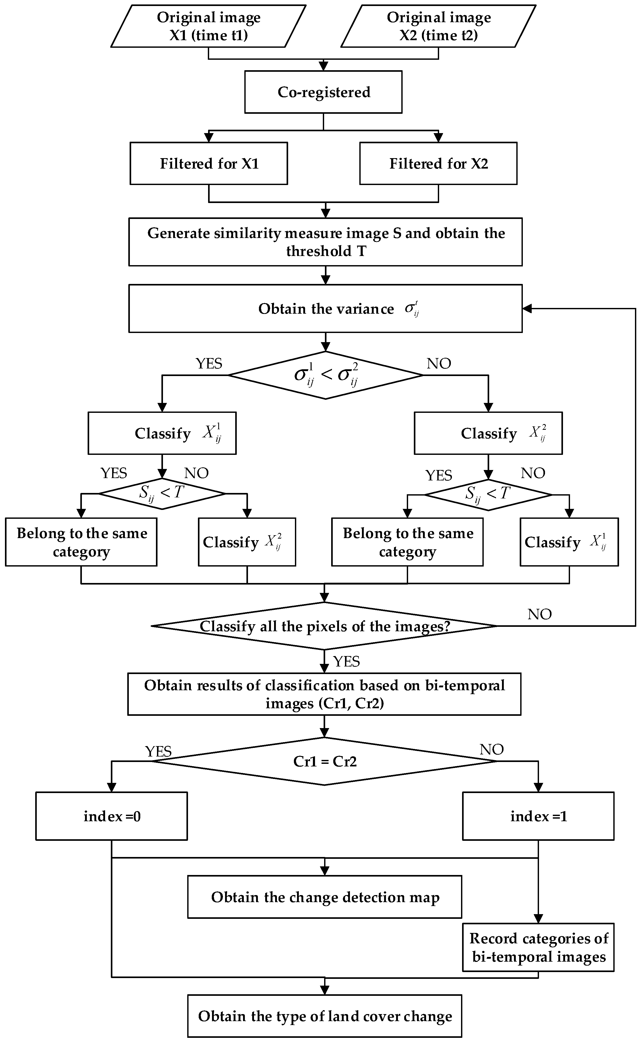
2.6. The Proposed JCC-TSKI Method

The entire procedure of the proposed method is as follows:
Step 1
The bi-temporal PolSAR images should be co-registered and filtered. Image registration is performed to align the images used in the change detection. Speckle filtering is commonly used to suppress speckle noise before the change detection and classification of PolSAR images. The preprocessing is important for change detection. In this study, Refined Lee filtering based on 7 × 7 windows was used to remove speckle noise [22].
Step 2
The similarity measure can be obtained through the test statistics (TS) using the coherence matrix of the bi-temporal images. In this step, bi-temporal fully PolSAR data are used to generate the S. Furthermore, K & I is used to select the optimum threshold for S.
Step 3
Variances of intensity σ i j 1 , σ i j 2 are used to determine the sequence of JCC-TSKI.
Step 4
If σ i j 1 < σ i j 2 , we choose X1 to be firstly classified; otherwise, we choose X2 to be firstly classified.
Step 5
Determine the category of position ( i , j ) . If S i j < T , this means that the bi-temporal PolSAR data in the same position is similar, and the class label in the corresponding pixel position of another time concurs with the reference; otherwise, we classify the corresponding pixel position of the other time on its own.
Step 6
Check whether all the pixels of the bi-temporal PolSAR images are classified or not. If not, move to the next pixel, and return to step 3; otherwise, obtain the results of classification based on bi-temporal images.
Step 7
Check whether class labels of bi-temporal images are equal or not. If not, record the labels, and consider index = 1; otherwise, consider index = 0.
Step 8
We can obtain the change detection map by the value of index and the type of land cover change by the record of labels.
The detailed process flow of JCC-TSKI is shown in Figure 1.

2.7. Evaluation Criterion

Quantitative evaluation is important to determine the result of the change detection. When the ground truth is available, a quantitative evaluation can be performed [42,44]. In order to verify the performance of the proposed method, we calculated the false alarm (FA) rate, total errors (TE), overall accuracy (OA), and Kappa coefficient [45] of the experimental results. These indicators are calculated as follows:
{ F A = F P N u N = N u + N c T E = F P + F N N , O A = T P + T N N K a p p a = O A P e 1 P e P e = ( T P + F N ) ( T P + F P ) + ( F P + T N ) ( F N + T N ) N 2 ,
where TP (true positives) means the number of changed points correctly detected; TN (true negatives) means the number of unchanged points correctly detected; FP (false positives) means the number of unchanged points incorrectly detected as changed (false alarm); and FN (false negatives) means the number of changed points incorrectly detected as unchanged (missed detections). N u and N c are the number of unchanged points and changed points of the ground-truth change map, respectively.

3. Results and Discussion

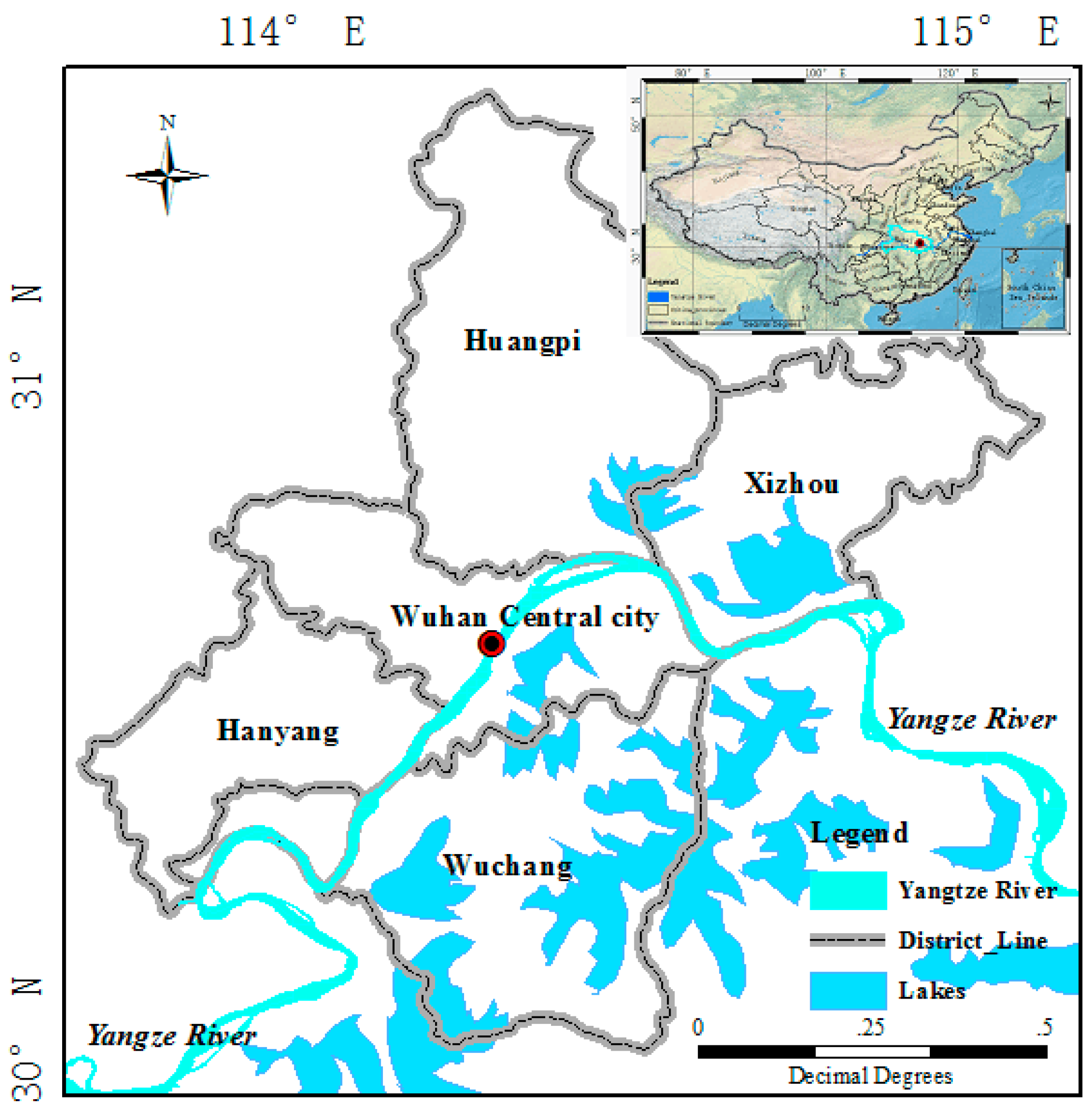
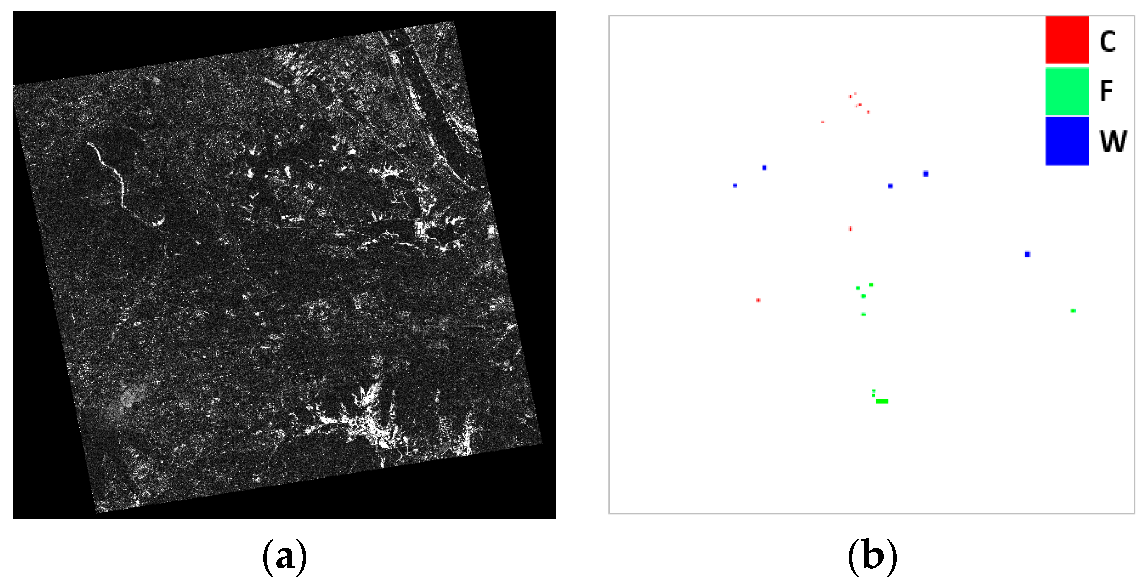
3.1. Study Area and Background

The city of Wuhan is in the east of Hubei province and lies in the eastern Jianghan Plain, at the intersection of the middle reaches of the Yangtze (Figure 2). Its climate is humid subtropical, with abundant rainfall and four distinctive seasons. In July 2016, a 50-year return period of rainfall occurred, and the rainfall was significantly higher than the average annual precipitation. Wuhan was affected by the continuous heavy rain, and some areas were seriously flooded and dramatically changed. The use of optical sensors was limited by this severe weather. In order to detect the flooded regions, bi-temporal PolSAR images can acquire not only the region of change, but can also detect the type of land cover change (e.g., surface features changed to water), allowing a rapid emergency response.

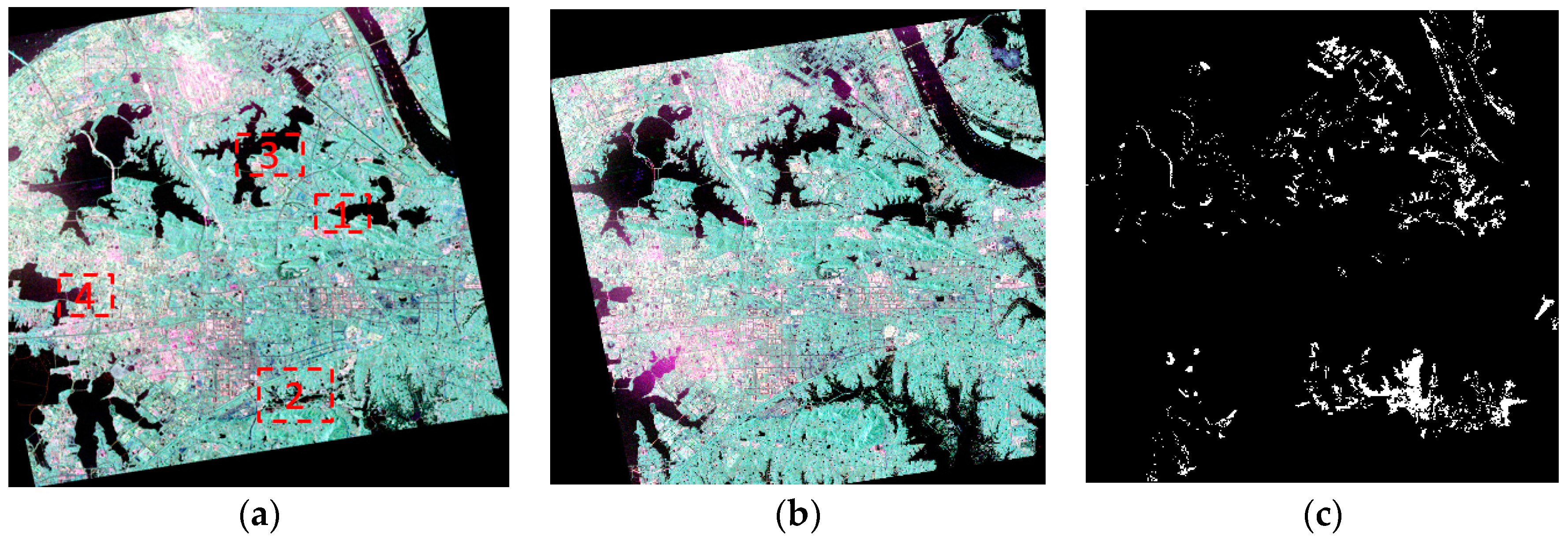
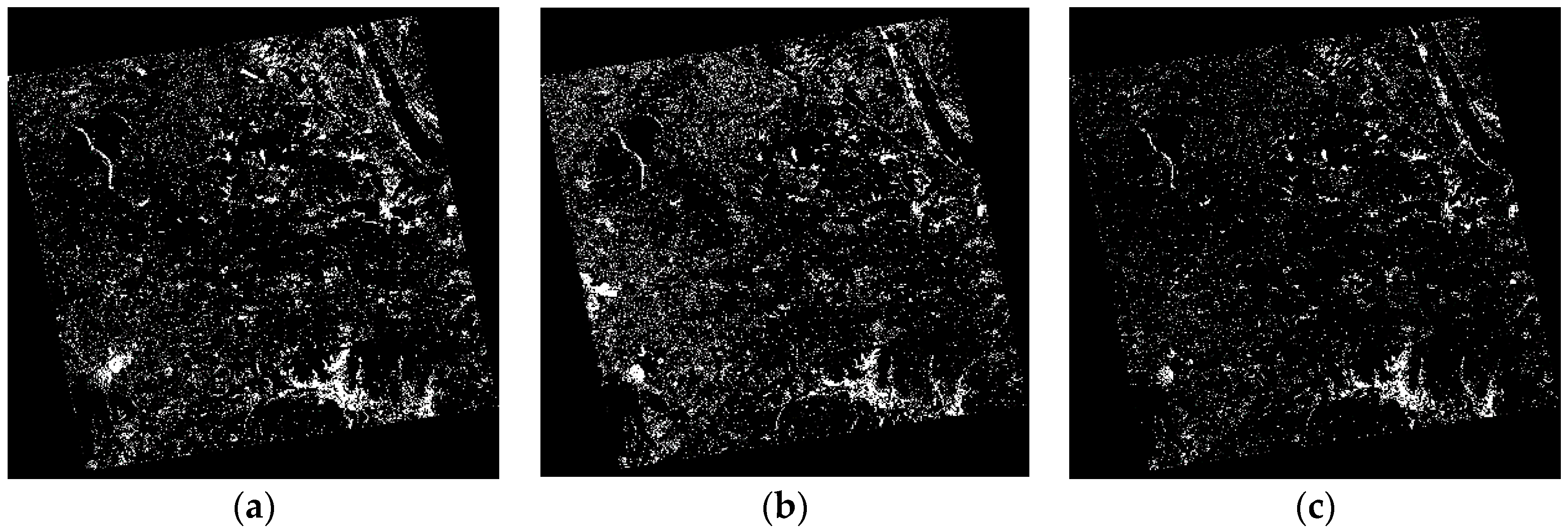
3.2. RADARSAT-2 Images and Preprocessing

Two C-band quad-polarimetric RADARSAT-2 (single look complex) images of Wuhan were acquired on 25 June 2015 and 6 July 2016. The nominal pixel spacings in the azimuth and range directions were 5.12 × 4.73 m and 4.86 × 4.73 m, respectively. The swath width was 25 × 25 km, and the beams of the images were FQ21 and FQ27, with the incidence angle ranging from 40.16 to 41.58° and 45.23 to 46.49°, respectively. The repeat cycle was 24 days. The preprocessing consisted of radiometric calibration, speckle filtering, and image co-registration. After the radiometric calibration, the pixel values of the bi-temporal PolSAR images are directly related to the radar backscatter of the scene. This condition is necessary for the comparison of PolSAR images acquired at different dates. Image co-registration and speckle filtering are performed. Image co-registration is aimed at reducing the errors caused by the mis-registration of the images. Two free open-source software packages—the Next ESA SAR Toolbox (NEST) [46] and the PolSARpro SAR Data Processing and Educational Tool [47]—were used in the preprocessing of the SAR datasets. The co-registration image sizes are 4906 × 5114 pixels.
The Pauli-RGB images ( | S h h S v v | for red (R), | S h v | for green (G), and | S h h + S v v | for blue (B)) are shown in Figure 3a,b. The regions labeled by the four red boxes in the Figure 3a are used to give a detailed assessment. All of these regions have a common characteristic, i.e., containing water bodies. The ground reference is shown in Figure 3c, displaying corresponding optical images obtained by Google Earth (version 7.1.8) and field surveys conducted by researchers.

3.3. Result of Change Detection in the Bi-Temporal PolSAR Images

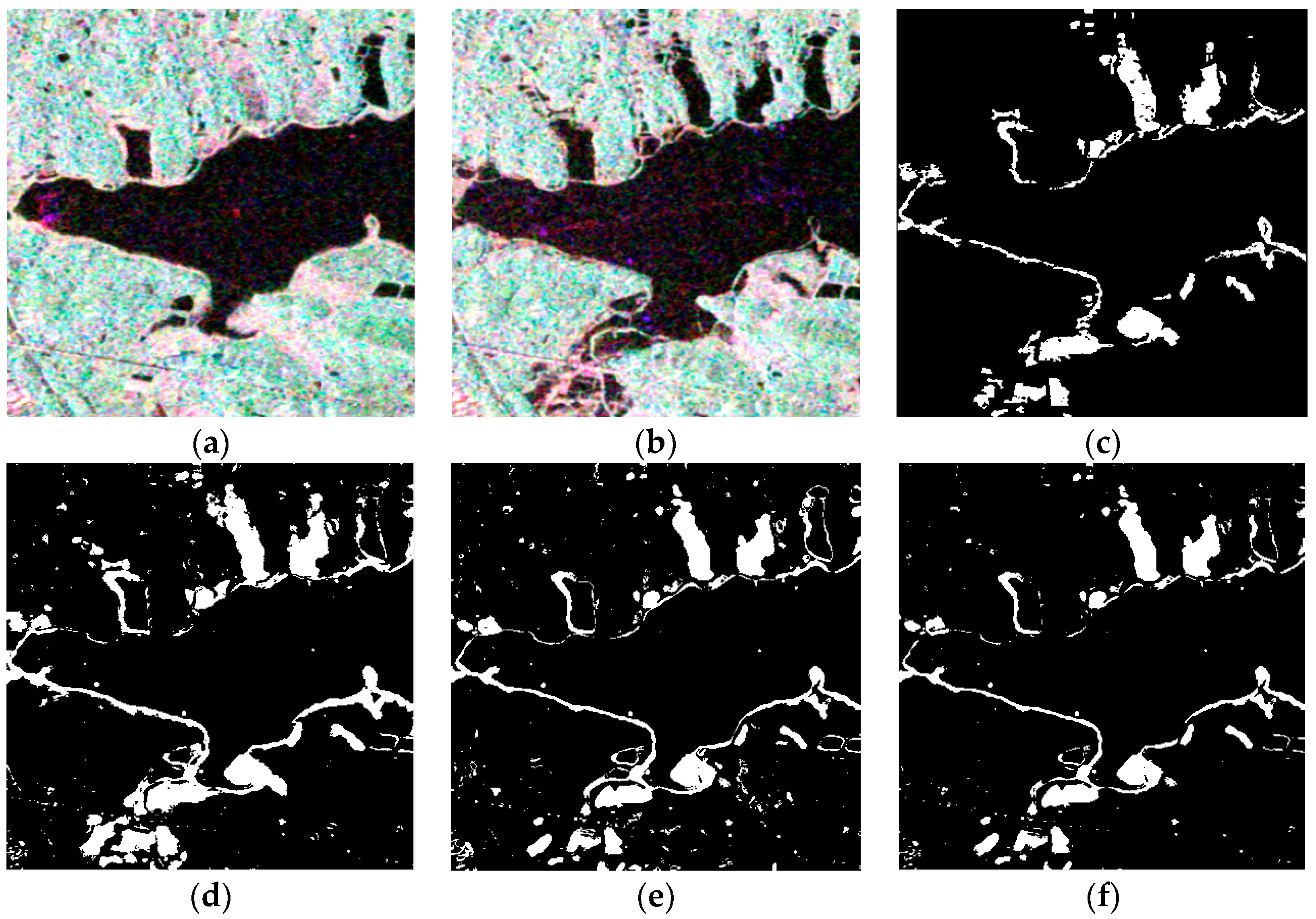
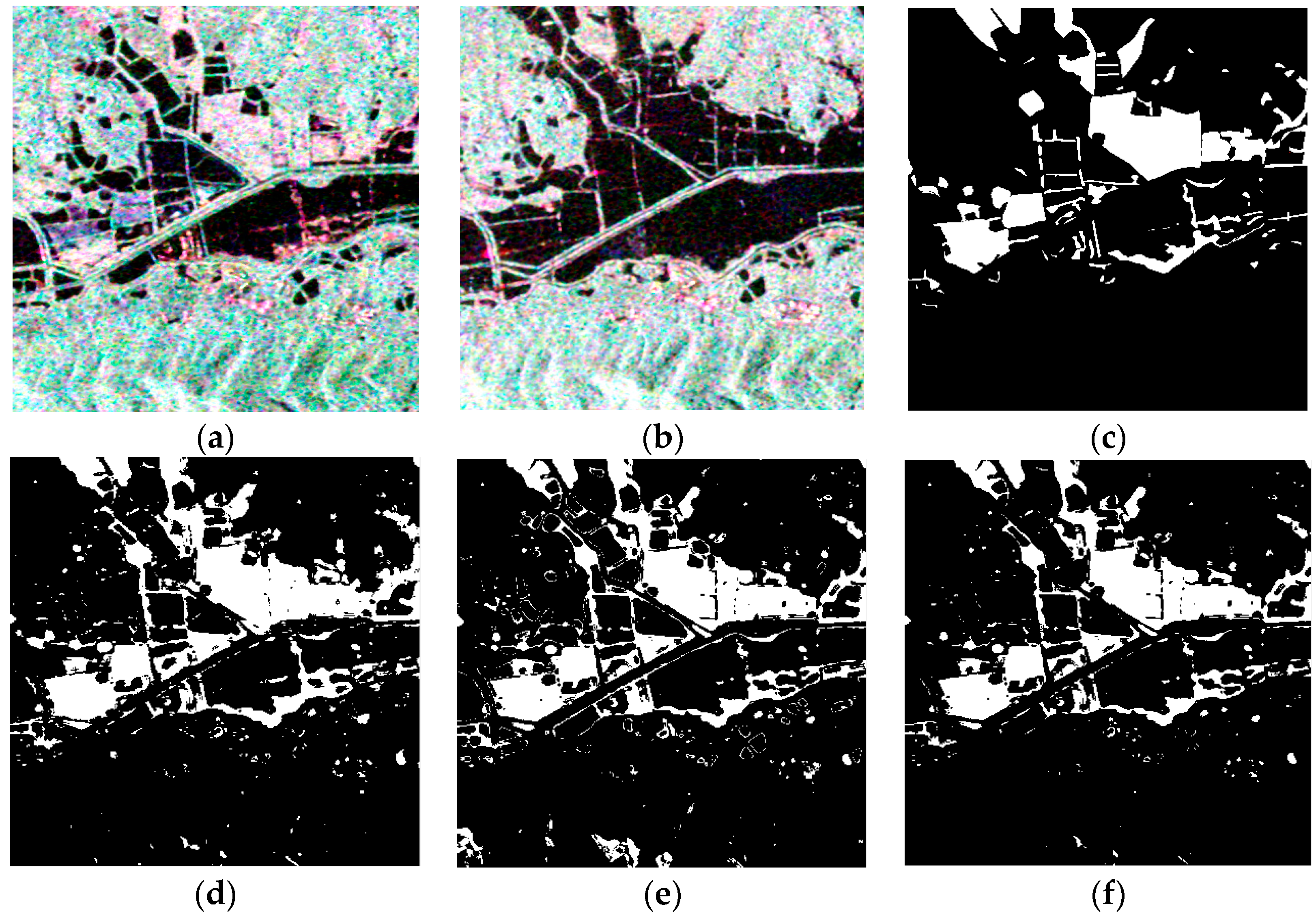
3.3.1. Similarity Measures

The results of the S based on the test statistics were adjusted to the range [0, 1] by linear mapping, as shown in Figure 4a. Using the automatic threshold method of K & I, the optimal threshold value was 0.53. In this experiment, we focused on the water change. Therefore, we only classified the bi-temporal PolSAR data into three categories: city (C), forest (F), and water (W). The chosen training samples included 3755 points of city (red), 11,784 points of forest (green), and 9750 points of water (blue), as shown in Figure 4b.

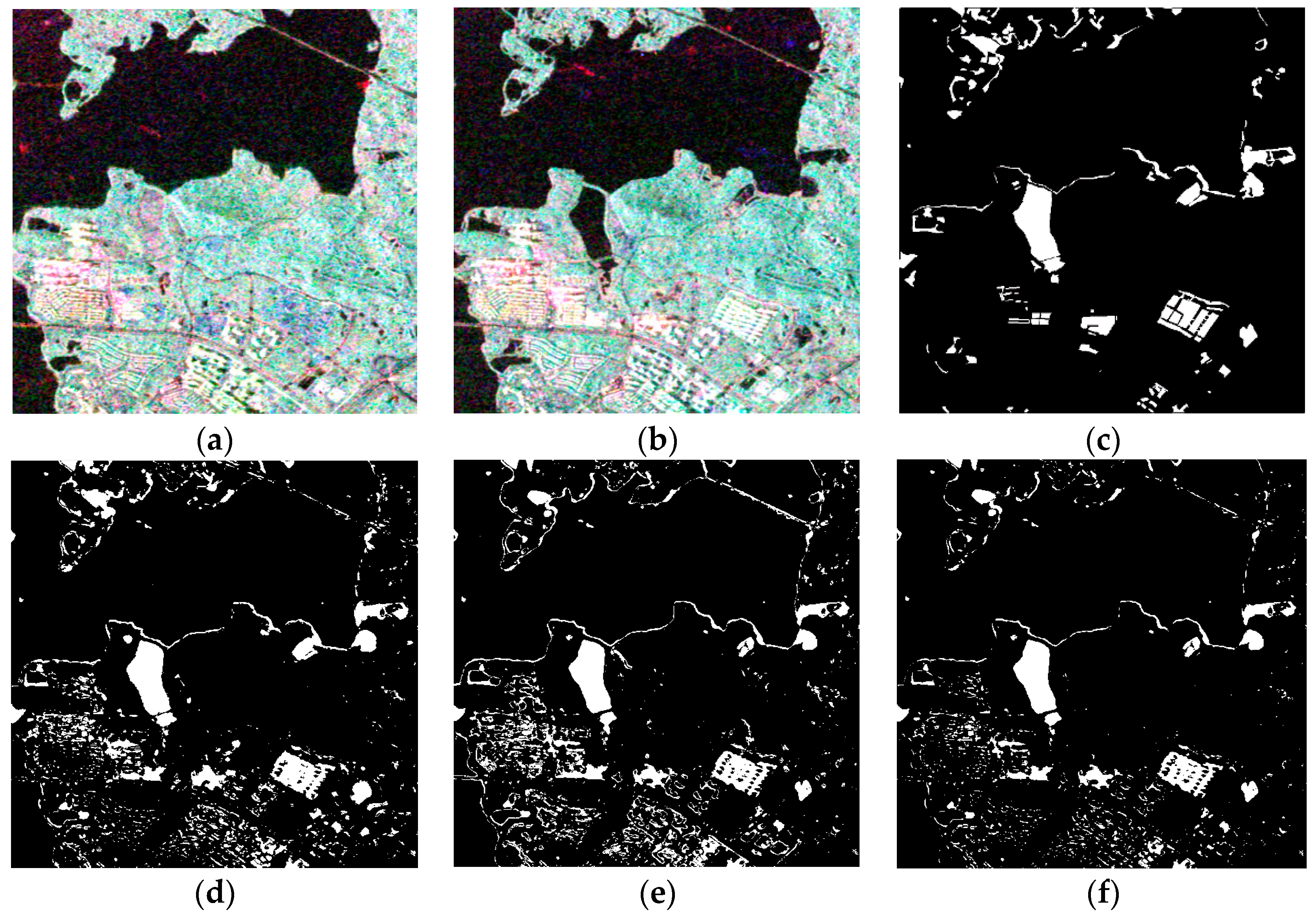
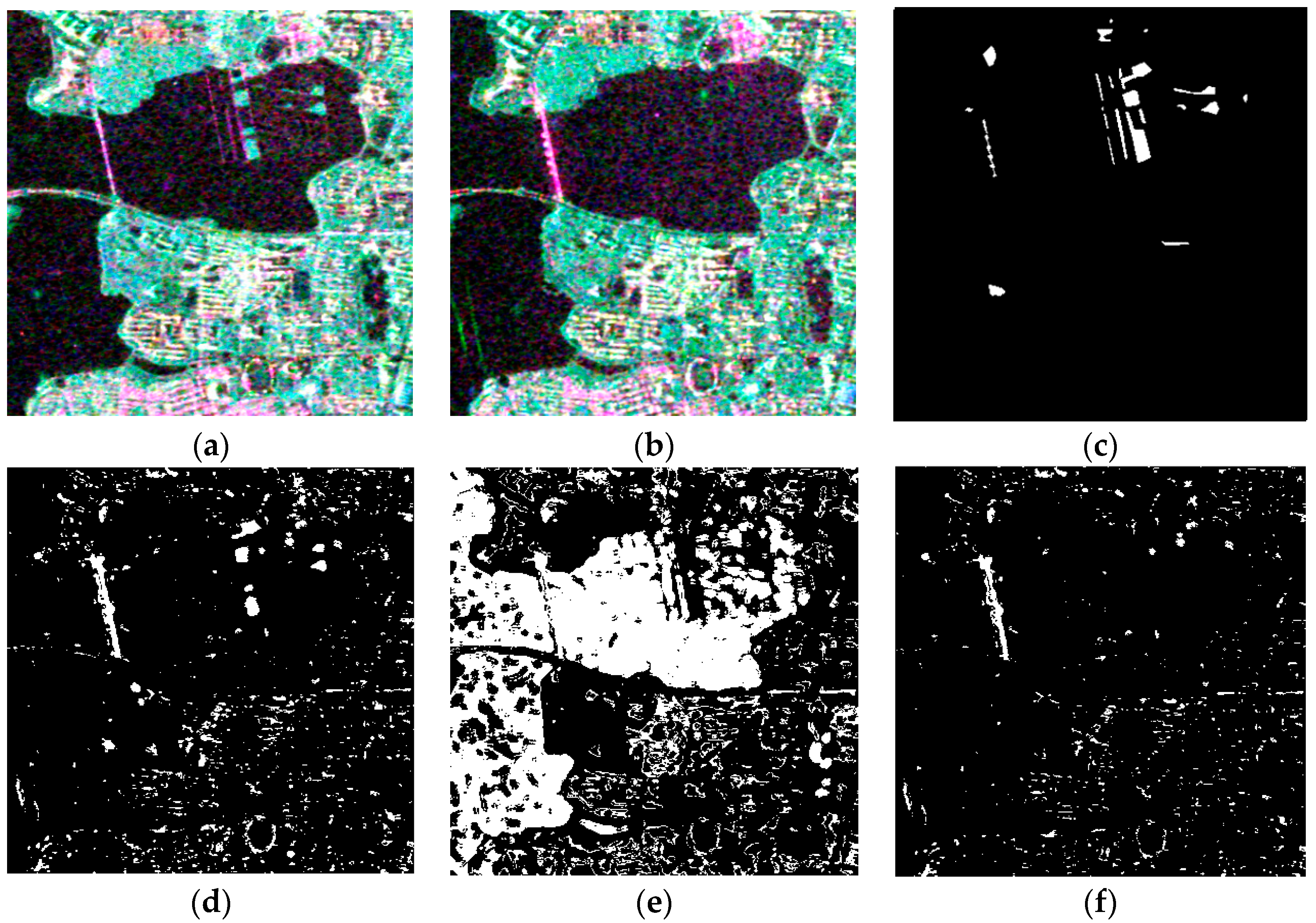
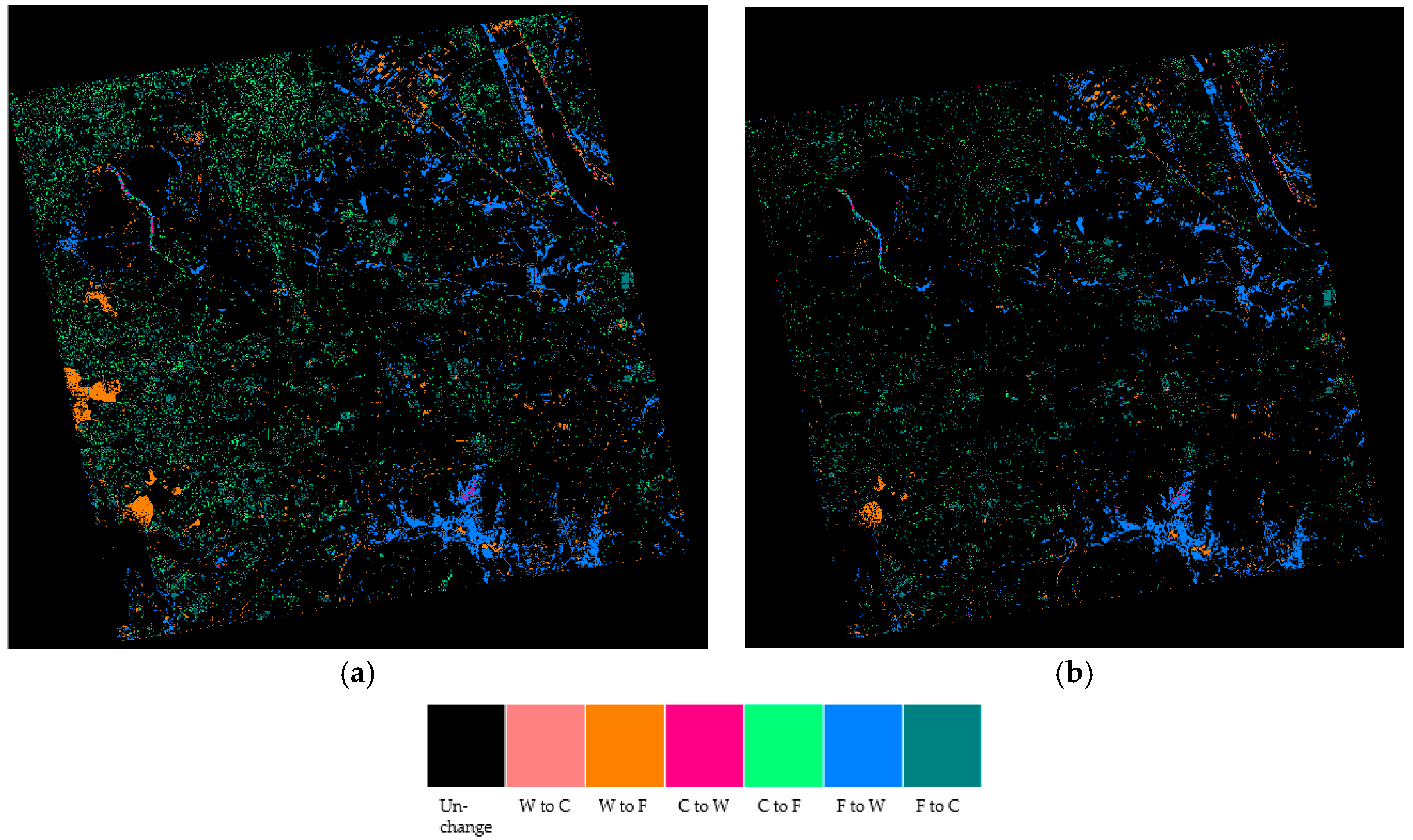
3.3.2. Experimental Results

After obtaining the necessary parameters described above, we could obtain the result of change detection based on the proposed method. In order to verify the efficiency of the proposed method, comparative experiments were designed. We compared unsupervised change detection based on TSKI, supervised change detection based on PCC using the Wishart classifier, and the proposed method. The results for the bi-temporal PolSAR images of Wuhan are shown in Figure 5. The change detection maps show change (white) and non-change (black) information. The computational time for TSKI, PCC, and our method are 253 s, 242 s, and 301 s, respectively.
In Figure 5a, the result of unsupervised change detection based on TSKI can accurately reflect the changes, but it has a high false alarm rate. As another drawback, the details of the changes are not maintained well. In Figure 5b, the result of PCC based on the Wishart classifier can reflect the type of land cover change, but PCC depends on the result of classification of the bi-temporal PolSAR images, and the result contains many incorrect detections and a high false alarm rate. The result of the proposed method is shown in Figure 5c, where it can be seen that the proposed method not only preserves some of the details, but it also corrects the incorrect detection of PCC. As a result of adding the similarity measure in JCC-TSKI, the similar parts are retained, and the different parts are checked again by the type category of the classification of the bi-temporal PolSAR images. The proposed method is effective at preserving the detail and decreasing the false alarms. As we focus on the change in the highlighted regions in Figure 3, these areas are chosen to give detailed assessments.
The areas of YanDong Lake (region 1 of the Figure 3a,) and LiangZi Lake (region 2 of the Figure 3a, 400 × 400 pixels) have similar surface features. Moreover, the main changes of these parts occurred in the water area because of the rain. Results of these regions are shown in Figure 6 and Figure 7. The three methods were all able to detect the main changes. However, the results of TSKI and PCC contain many false alarms. Because of the large difference in the backscattering of these land cover types, it is easy to classify these categories. Therefore, PCC based on the Wishart classifier shows a good performance in maintaining the details, but it still shows some weaknesses, including incorrect detections and false alarms. TSKI also has a problem of high false alarms. The proposed method shows a significant improvement in decreasing the false alarms, and maintains the details of the change information of the water bodies.
The quantitative comparison of the three detection schemes shown in Table 1 and Table 2 also indicates that the proposed approach shows a better performance. The proposed approach achieves the best results in four indicators (FA (%), TE (%), OA (%), KAPPA). Moreover, the proposed method not only shows a significant improvement in decreasing the false alarms over the unsupervised method and can detect the type of land cover change, it also obtains fewer incorrect detections and false alarms than PCC. This confirms that the proposed method is effective and shows a significant improvement over PCC and TSKI.
The areas of YanXi Lake (region 3 of the Figure 3a, 600 × 600 pixels) includes grassland, city, and water bodies. The main changes not only occurred in the water area as a result of the rain, but also occurred in the city area. Results of these regions are shown in Figure 8. The three methods were all able to detect the main changes. However, the results of TSKI and PCC contain many false alarms. Because of the large differences in the backscattering of these land cover types, it is easy to classify these categories. Therefore, PCC based on the Wishart classifier shows a good performance in maintaining the detail, but it still has some weaknesses, such as incorrect detections and false alarms. TSKI also has the problem of a high false alarm rate. The proposed method shows a significant improvement in decreasing the false alarms, and maintains the details of the change information of the water bodies and city area. The quantitative comparison of the three detection schemes shown in Table 3 indicates that the proposed approach shows a better performance. The proposed approach achieves the best results in four indicators (FA (%), TE (%), OA (%), KAPPA). Above all, these experimental analyses show that our proposed method is suitable for detecting the changes in both water and part of city areas.
The area of Nan Lake (region 4 of the Figure 3a, 400 × 400 pixels) consists of water, bridge and city. Because of the impacts of the surrounding buildings, Nan Lake appears different in Figure 9a,b. However, the water body of Nan Lake has been keeping the same for the two acquisitions. Results of these regions are shown in Figure 9. Because of different results of classifications in this part of bi-temporal PolSAR images, the PCC method considers this region as changed. Because of the inclusion of similarity measure in our method, the results of TSKI and the proposed method correct this incorrect detection, marking this area as unchanged. However, due to the same classifier used in PCC and JCC, some changed parts in the ground truth are put into the same category in the same classification result. This causes some missed detection. This result demonstrates that the proposed method obtains fewer incorrect detections than PCC, and has a lower false alarm rate than PCC and TSKI. As it can be clearly seen that the result of PCC in Figure 9e contains many incorrect detections, we did not need to undertake a quantitative comparison between PCC and our proposed method in this region.
As a result of adding the similarity measure in the proposed method, it decreases the rate of incorrect detection and the false alarm rate, and shows a dramatic improvement over PCC. Compared to TSKI, the similar parts are retained, and the different parts are checked again by the type category of the bi-temporal PolSAR data in JCC-TSKI. This can preserve the details and decrease the false alarms. Moreover, our proposed method can detect the type of land cover change.
Compared with the unsupervised method of change detection, the supervised method of change detection can detect the type of land cover change, as shown in Figure 10. Because PCC is affected by the cumulative error of the single remote image classification, the PCC result contains many incorrect detections and false alarms. In Figure 10a, the change types of forest to city (F to C) and city to forest (C to F) are the main changes in PCC. As a result of the low backscatter of water, it is easy to classify the water by means of the Wishart classifier. The PCC method shows a good performance in detecting the change types of forest to lake and city to lake. The results of the proposed method show the advantage of detecting the changes of water regions and decreasing the incorrect detections and false alarms. In Figure 10b, the change types of forest to city and city to forest are decreased, and the results show a dramatic improvement. Due to large study areas and inclement weather conditions, the map of land cover change over a couple of days is not available. Therefore, the quantification for the type of land cover change is difficult to achieve.

4. Conclusions

In this paper, we have presented a novel bi-temporal PolSAR image change detection approach. A similarity measure and JCC are used to deal with the challenges faced by both the unsupervised and supervised change detection approaches. Bi-temporal PolSAR images are used in the proposed method. Unlike other change detection approaches using bi-temporal single-channel SAR images, the proposed method applies the bi-temporal fully PolSAR images to detect the changes. As a result of using the information of the PolSAR data, it is easier to detect the slight differences. We use TSKI to obtain the similarity measure. This can make use of all the PolSAR information and automatically choose the threshold of the test statistic and Kittler and Illingworth algorithm. The similarity measure used in the proposed method can determine the similarity of the same region at different times, and can distinguish both similar and different parts. We consider the similar parts as the same category, and the different parts are classified, respectively. Because the backscatter of water is low, it is easy to distinguish using the Wishart classifier. The results of the proposed method are more effective and accurate. This paper describes a novel change detection process. Thus, we believe that the proposed method will be a practical solution for unsupervised change detection. The experimental results include the change type information and contain fewer false alarms than TSKI. The proposed method also solves some of the problems of supervised change detection, such as the high level of incorrect detections and false alarms. In the experiments, the proposed method showed a dramatic improvement over PCC.

Acknowledgments

The authors would like to thank the National Natural Science Foundation of China (Grant No. 91438203, No. 61371199, No. 41501382, and No. 41601355); the Public Welfare Project of Surveying and Mapping Interest (201412002); the Hubei Provincial Natural Science Foundation (No. 2015CFB328, No. 2016CFB246); the National Basic Technology Program of Surveying and Mapping (No. 2016KJ0103); and the Technology of Target Recognition Based on GF-3 Program (No. 03-Y20A10-9001-15/16). The figures and analysis in our study were generated and performed by VS2010 and Matlab2015.

Author Contributions

Jinqi Zhao defined the research problem, proposed the method, undertook most of the programming in Matlab and VS2010, and wrote the paper; Jie Yang gave some key advice; Zhong Lu gave useful advice and contributed to the paper writing; Pingxiang Li provided the RADARSAT-2 data and some useful advice; Wensong Liu collected the data and processed the datasets in ENVI (version 5.1), PolSARpro (version 4.2.0), and NEST software (version 5.1); Le Yang obtained the ground-truth map.

Conflicts of Interest

The authors declare no conflict of interest.

References

  1. Singh, A. Review article digital change detection techniques using remotely-sensed data. Int. J. Remote Sens. 1989, 10, 989–1003. [Google Scholar] [CrossRef]
  2. Bruzzone, L.; Bovolo, F. A novel framework for the design of change-detection systems for very-high-resolution remote sensing images. IEEE Proc. 2013, 101, 609–630. [Google Scholar] [CrossRef]
  3. Anaya, J.A.; Colditz, R.R.; Valencia, G.M. Land Cover Mapping of a Tropical Region by Integrating Multi-Year Data into an Annual Time Series. Remote Sens. 2015, 7, 16274–16292. [Google Scholar] [CrossRef] [Green Version]
  4. Zhao, J.Q.; Yang, J.; Li, P.X.; Liu, M.Y.; Shi, Y.M. An Unsupervised Change Detection Based on Test Statistic and KI from Multi-temporal and Full Polarimetric SAR Images. Int. Arch. Photogramm. Remote Sens. Spat. Inf. Sci. 2016, XLI-B7, 611–615. [Google Scholar] [CrossRef]
  5. Conradsen, K.; Nielsen, A.A.; Schou, J.; Skriver, H. A test statistic in the complex Wishart distribution and its application to change detection in polarimetric SAR data. IEEE Trans. Geosci. Remote Sens. 2003, 41, 4–19. [Google Scholar] [CrossRef]
  6. Lu, Z.; Kwoun, O. Radarsat-1 and ERS InSAR analysis over southeastern coastal Louisiana: Implications for mapping water-level changes beneath swamp forests. IEEE Trans. Geosci. Remote Sens. 2008, 46, 2167–2184. [Google Scholar] [CrossRef]
  7. Zhao, L.L.; Yang, J.; Li, P.X.; Zhang, L.P. Seasonal inundation monitoring and vegetation pattern mapping of the Erguna floodplain by means of a RADARSAT-2 fully polarimetric time series. Remote Sens. Environ. 2014, 152, 426–440. [Google Scholar] [CrossRef]
  8. Huang, C.Q. Forest Change Analysis Using Time-Series Landsat Observations. In Advances in Environmental Remote Sensing: Sensors, Algorithms, and Applications; CRC Press: Boca Raton, FL, USA, 2011; pp. 339–365. [Google Scholar]
  9. Kwoun, O.-I.; Lu, Z. Multi-temporal RADARSAT-1 and ERS backscattering signatures of coastal wetlands in southeastern Louisiana. Photogramm. Eng. Remote Sens. 2009, 75, 607–617. [Google Scholar] [CrossRef]
  10. Celik, T. Unsupervised change detection in satellite images using principal component analysis and k-means clustering. IEEE Geosci. Remote Sens. Lett. 2009, 6, 772–776. [Google Scholar] [CrossRef]
  11. Song, D.-X.; Huang, C.Q.; Sexton, J.O.; Channan, S.; Feng, M.; Townshend, J.R. Use of Landsat and Corona data for mapping forest cover change from the mid-1960s to 2000s: Case studies from the Eastern United States and Central Brazil. ISPRS J. Photogramm. Remote Sens. 2015, 103, 81–92. [Google Scholar] [CrossRef]
  12. Sun, W.D.; Shi, L.; Yang, J.; Li, P.X. Building collapse assessment in urban areas using texture information from postevent SAR data. IEEE J. Sel. Top. Appl. Earth Obs. Remote Sens. 2016, 9, 3792–3808. [Google Scholar] [CrossRef]
  13. Zhao, L.L.; Yang, J.; Li, P.X.; Zhang, L.P.; Shi, L.; Lang, F.K. Damage assessment in urban areas using post-earthquake airborne PolSAR imagery. Int. J. Remote Sens. 2013, 34, 8952–8966. [Google Scholar] [CrossRef]
  14. Zhao, L.L.; Yang, J.; Li, P.X.; Zhang, L.P. Characteristics analysis and classification of crop harvest patterns by exploiting high-frequency multipolarization SAR data. IEEE J. Sel. Top. Appl. Earth Obs. Remote Sens. 2014, 7, 3773–3783. [Google Scholar] [CrossRef]
  15. Lu, Z.; Dzurisin, D. InSAR imaging of Aleutian volcanoes. In InSAR Imaging of Aleutian Volcanoes; Springer: Berlin, Germany, 2014; pp. 87–345. [Google Scholar]
  16. Novellino, A.; Cigna, F.; Sowter, A.; Ramondini, M.; Calcaterra, D. Exploitation of the Intermittent SBAS (ISBAS) algorithm with COSMO-SkyMed data for landslide inventory mapping in north-western Sicily, Italy. Geomorphology 2017, 280, 153–166. [Google Scholar] [CrossRef]
  17. Rignot, E.J.; van Zyl, J.J. Change detection techniques for ERS-1 SAR data. IEEE Trans. Geosci. Remote Sens. 1993, 31, 896–906. [Google Scholar] [CrossRef]
  18. Bazi, Y.; Bruzzone, L.; Melgani, F. An unsupervised approach based on the generalized Gaussian model to automatic change detection in multitemporal SAR images. IEEE Trans. Geosci. Remote Sens. 2005, 43, 874–887. [Google Scholar] [CrossRef]
  19. Moser, G.; Serpico, S.B. Generalized minimum-error thresholding for unsupervised change detection from SAR amplitude imagery. IEEE Trans. Geosci. Remote Sens. 2006, 44, 2972–2982. [Google Scholar] [CrossRef]
  20. Sumaiya, M.; Kumari, R.S.S. Logarithmic Mean-Based Thresholding for SAR Image Change Detection. IEEE Geosci. Remote Sens. Lett. 2016, 13, 1726–1728. [Google Scholar] [CrossRef]
  21. Liu, M.; Zhang, H.; Wang, C.; Wu, F. Change detection of multilook polarimetric SAR images using heterogeneous clutter models. IEEE Trans. Geosci. Remote Sens. 2014, 52, 7483–7494. [Google Scholar]
  22. Lee, J.-S.; Jurkevich, L.; Dewaele, P.; Wambacq, P.; Oosterlinck, A. Speckle filtering of synthetic aperture radar images: A review. Remote Sens. Rev. 1994, 8, 313–340. [Google Scholar] [CrossRef]
  23. Cozzolino, D.; Parrilli, S.; Scarpa, G.; Poggi, G.; Verdoliva, L. Fast adaptive nonlocal SAR despeckling. IEEE Geosci. Remote Sens. Lett. 2014, 11, 524–528. [Google Scholar] [CrossRef]
  24. Carincotte, C.; Derrode, S.; Bourennane, S. Unsupervised change detection on SAR images using fuzzy hidden Markov chains. IEEE Trans. Geosci. Remote Sens. 2006, 44, 432–441. [Google Scholar] [CrossRef]
  25. Bouyahia, Z.; Benyoussef, L.; Derrode, S. Change detection in synthetic aperture radar images with a sliding hidden Markov chain model. J. Appl. Remote Sens. 2008, 2, 023526. [Google Scholar] [Green Version]
  26. Inglada, J.; Mercier, G. A new statistical similarity measure for change detection in multitemporal SAR images and its extension to multiscale change analysis. IEEE Trans. Geosci. Remote Sens. 2007, 45, 1432–1445. [Google Scholar] [CrossRef]
  27. Akbari, V.; Anfinsen, S.N.; Doulgeris, A.P.; Eltoft, T.; Moser, G.; Serpico, S.B. Polarimetric SAR Change Detection With the Complex Hotelling—Lawley Trace Statistic. IEEE Trans. Geosci. Remote Sens. 2016, 54, 3953–3966. [Google Scholar] [CrossRef]
  28. Zhang, Y.; Wu, H.A.; Wang, H.; Jin, S. Distance Measure Based Change Detectors for Polarimetric SAR Imagery. Photogramm. Eng. Remote Sens. 2016, 82, 719–727. [Google Scholar] [CrossRef]
  29. Bunch, J.R.; Fierro, R.D. A constant-false-alarm-rate algorithm. Linear Algebra Its Appl. 1992, 172, 231–241. [Google Scholar] [CrossRef]
  30. Otsu, N. A threshold selection method from gray-level histograms. Automatica 1975, 11, 23–27. [Google Scholar] [CrossRef]
  31. Kapur, J.N.; Sahoo, P.K.; Wong, A.K. A new method for gray-level picture thresholding using the entropy of the histogram. Comput. Vis. Graph. Image Proc. 1985, 29, 273–285. [Google Scholar] [CrossRef]
  32. Kittler, J.; Illingworth, J. Minimum error thresholding. Pattern Recognit. 1986, 19, 41–47. [Google Scholar] [CrossRef]
  33. Qi, Z.; Yeh, A.G.O.; Li, X.; Zhang, X.H. A three-component method for timely detection of land cover changes using polarimetric SAR images. ISPRS J. Photogramm. Remote Sens. 2015, 107, 3–21. [Google Scholar] [CrossRef]
  34. Zhou, W.; Troy, A.; Grove, M. Object-based land cover classification and change analysis in the Baltimore metropolitan area using multitemporal high resolution remote sensing data. Sensors 2008, 8, 1613–1636. [Google Scholar] [CrossRef] [PubMed]
  35. Han, M.; Zhou, Y. Joint-classification change detection based on improved fuzzy ARTMAP. In Proceedings of the 2015 IEEE International Geoscience and Remote Sensing Symposium (IGARSS), Milan, Italy, 26–31 July 2015. [Google Scholar]
  36. Gomez, L.; Alvarez, L.; Mazorra, L.; Frery, A.C. Classification of complex Wishart matrices with a diffusion—Reaction system guided by stochastic distances. Philos. Trans. R. Soc. A 2015, 373, 20150118. [Google Scholar] [CrossRef] [PubMed]
  37. Lee, J.-S.; Grunes, M.R.; Kwok, R. Classification of multi-look polarimetric SAR imagery based on complex Wishart distribution. Int. J. Remote Sens. 1994, 15, 2299–2311. [Google Scholar] [CrossRef]
  38. Huang, C.; Davis, L.; Townshend, J. An assessment of support vector machines for land cover classification. Int. J. Remote Sens. 2002, 23, 725–749. [Google Scholar] [CrossRef]
  39. Mountrakis, G.; Im, J.; Ogole, C. Support vector machines in remote sensing: A review. ISPRS J. Photogramm. Remote Sens. 2011, 66, 247–259. [Google Scholar] [CrossRef]
  40. Li, J.-J.; Jiao, L.C.; Zhang, X.R.; Yang, D.D. Change detection for SAR images based on joint-classification of bi-temporal images. J. Infrared Millim. Waves 2009, 6, 015. [Google Scholar] [CrossRef]
  41. Lee, J.-S.; Grunes, M.R.; Ainsworth, T.L.; Du, L.-J.; Schuler, D.L.; Cloude, S.R. Unsupervised classification using polarimetric decomposition and the complex Wishart classifier. IEEE Trans. Geosci. Remote Sens. 1999, 37, 2249–2258. [Google Scholar]
  42. Yang, W.; Yang, X.L.; Yan, T.H.; Song, H.; Xia, G.S. Region-Based Change Detection for Polarimetric SAR Images Using Wishart Mixture Models. IEEE Trans. Geosci. Remote Sens. 2016, 54, 6746–6756. [Google Scholar] [CrossRef]
  43. Lee, J.-S.; Pottier, E. Polarimetric Radar Imaging: From Basics to Applications; CRC Press: Boca Raton, FL, USA, 2009. [Google Scholar]
  44. Pham, M.-T.; Mercier, G.; Michel, J. Change detection between SAR images using a pointwise approach and graph theory. IEEE Trans. Geosci. Remote Sens. 2016, 54, 2020–2032. [Google Scholar] [CrossRef]
  45. Stehman, S.V. Selecting and interpreting measures of thematic classification accuracy. Remote Sens. Environ. 1997, 62, 77–89. [Google Scholar] [CrossRef]
  46. ESA. The PolSARpro SAR Data Processing and Educational Tool. Available online: https://earth.esa.int/web/polsarpro/home (accessed on 29 May 2017).
  47. ESA. The Next ESA SAR Toolbox. Available online: http://nest.array.ca/web/nest (accessed on 29 May 2017).
Figure 1. The flow chart of Joint-Classification Classifier based on Test statistics and the Kittler and Illingworth (JCC-TSKI).
Remotesensing 09 00846 g001
Figure 2. Location of the study areas.
Remotesensing 09 00846 g002
Figure 3. The Pauli-RGB images of Wuhan after preprocessing, for (a) 25 June 2015; and (b) 6 July 2016; (c) the ground reference (white denotes the change and black denotes the non-change). In (a), region 1 is YanDong Lake, region 2 is LiangZi Lake, region 3 is YanXi Lake, and region 4 is Nan Lake.
Remotesensing 09 00846 g003
Figure 4. (a) the result of S; (b) training samples.
Remotesensing 09 00846 g004
Figure 5. The result of the change detection: (a) test statistics and the Kittler and Illingworth (TSKI); (b) post-classification comparison (PCC); and (c) the proposed method.
Remotesensing 09 00846 g005
Figure 6. RADARSAT-2 PolSAR images of the red box labeled area 1 acquired on (a) 25 June 2015; and (b) 6 July 2016; (c) the ground truth; change detection results of (d) TSKI; (e) PCC; and (f) JCC-TSKI.
Remotesensing 09 00846 g006
Figure 7. RADARSAT-2 PolSAR images of the red box labeled area 2 acquired on (a) 25 June 2015; and (b) 6 July 2016; (c) the ground truth; change detection results of (d) TSKI; (e) PCC; and (f) JCC-TSKI.
Remotesensing 09 00846 g007
Figure 8. RADARSAT-2 PolSAR images of the red box labeled area 3 acquired on (a) 25 June 2015; and (b) 6 July 2016; (c) the ground truth; change detection results of (d) TSKI; (e) PCC; and (f) JCC-TSKI.
Remotesensing 09 00846 g008
Figure 9. RADARSAT-2 PolSAR images of the red box labeled area 4 acquired on (a) 25 June 2015; and (b) 6 July 2016; (c) the ground truth; Change detection results of (d) TSKI; (e) PCC; and (f) JCC-TSKI.
Remotesensing 09 00846 g009
Figure 10. The type of land cover change detected by (a) PCC; and (b) the proposed method.
Remotesensing 09 00846 g010
Table 1. Performance evaluation of the change detection over YanDong Lake.
MethodFA (%)TE (%)OA (%)KAPPA
TSKI5.645.9294.080.6755
PCC4.05.6394.360.6460
JCC-TSKI2.524.4095.600.6997
FA, TE, OA, KAPPA denote the false alarm, total errors, overall accuracy and Kappa coefficient, respectively.
Table 2. Performance evaluation of the change detection over LiangZi Lake.
MethodFA (%)TE (%)OA (%)KAPPA
TSKI7.48.0591.950.7038
PCC7.48.9991.050.6608
JCC-TSKI4.686.8093.200.7249
Table 3. Performance evaluation of the change detection over YanXi Lake.
MethodFA (%)TE (%)OA (%)KAPPA
TSKI4.866.1993.810.5862
PCC5.567.5792.430.4919
JCC-TSKI2.685.0694.940.5927

