
Mapping Regional Urban Extent Using NPP-VIIRS DNB and MODIS NDVI Data

1
Faculty of Information Engineering, China University of Geosciences, No. 388 Lumo Road, Wuhan 430074, China
2
National Engineering Research Center of Geographic Information System, Wuhan 430074, China
3
State Key Laboratory of Vegetation and Environmental Change, Institute of Botany, Chinese Academy of Sciences, Beijing 100093, China
*
Author to whom correspondence should be addressed.
Remote Sens. 2017, 9(8), 862; https://doi.org/10.3390/rs9080862
Submission received: 21 June 2017
/
Revised: 5 August 2017
/
Accepted: 17 August 2017
/
Published: 21 August 2017
(This article belongs to the Special Issue Recent Advances in Remote Sensing with Nighttime Lights)
Abstract
:The accurate and timely monitoring of regional urban extent is helpful for analyzing urban sprawl and studying environmental issues related to urbanization. This paper proposes a classification scheme for large-scale urban extent mapping by combining the Day/Night Band of the Visible Infrared Imaging Radiometer Suite on the Suomi National Polar-orbiting Partnership Satellite (NPP-VIIRS DNB) and the Normalized Difference Vegetation Index from the Moderate Resolution Imaging Spectroradiometer products (MODIS NDVI). A Back Propagation (BP) neural network based one-class classification method, the Present-Unlabeled Learning (PUL) algorithm, is employed to classify images into urban and non-urban areas. Experiments are conducted in mainland China (excluding surrounding islands) to detect urban areas in 2012. Results show that the proposed model can successfully map urban area with a kappa of 0.842 on the pixel level. Most of the urban areas are identified with a producer’s accuracy of 79.63%, and only 10.42% the generated urban areas are misclassified with a user’s accuracy of 89.58%. At the city level, among 647 cities, only four county-level cities are omitted. To evaluate the effectiveness of the proposed scheme, three contrastive analyses are conducted: (1) comparing the urban map obtained in this paper with that generated by the Defense Meteorological Satellite Program/Operational Linescan System Nighttime Light Data (DMSP/OLS NLD) and MODIS NDVI and with that extracted from MCD12Q1 in MODIS products; (2) comparing the performance of the integration of NPP-VIIRS DNB and MODIS NDVI with single input data; and (3) comparing the classification method used in this paper (PUL) with a linear method (Large-scale Impervious Surface Index (LISI)). According to our analyses, the proposed classification scheme shows great potential to map regional urban extents in an effective and efficient manner.
1. Introduction
Urban land occupies a relatively small fraction of the Earth’s surface, but is the main area of human activities [1]. Rapid socio-economic development and population growth have greatly encouraged the expansion of urban land areas [2,3]. According to the World Bank, by the end of 2015, the global urbanization rate had hit 53.85%, a dramatic increase from 46.54% in 2000. If current trends continue, by 2030, urban land cover will grow by 1.2 million km2, nearly tripling the global urban land area of circa 2000 [4]. This increase has a high-probability of occurring in developing countries with a rapid pace of urbanization, such as China. Although urbanization is an effective promotion of social progress, urban expansion has inevitably caused numerous environmental problems, resulting in natural habitat loss, threatening biodiversity, affecting local climate, etc. [5,6,7,8,9,10,11]. It is essential to obtain timely and accurate information on urbanized areas to monitor the environmental and socioeconomic processes [12,13].
Land cover maps derived from remotely-sensed data are a valuable source for mapping urban area and monitoring urban dynamics [14,15,16,17,18,19]. Images with high or medium spatial resolution are commonly used for characterizing the urban structures due to their detailed spatial observations of cities [20,21,22]. However, the coverage range of one scene in a high or medium spatial resolution image is limited. For example, IKONOS collects high-resolution imagery at 1 and 4 m resolution, and the swath of a single scene is 11 km × 11 km. When applied at the regional scale (e.g., China, covering approximately 9.6 million km2), a large number of images is needed to cover the entire area. It is time consuming and labor intensive to process multi-fold pixels [23]. High- and medium-spatial resolution images are also frequently affected by cloud cover. It is challenging to select high-quality images around the same time for a large area. Additionally, the sensors collecting high- and medium-resolution images have a relatively long revisiting period. For example, Landsat sensors, providing medium-resolution imagery of 30 m, have a revisit rate at 16 days, which reduces the number of suitable images. Thus, at the national or continental scale, coarse imagery with wider swaths and higher revisit rates is the preferred imagery for macroscopically monitoring urban extents [24].
As the main data source of coarse images, the Moderate Resolution Imaging Spectroradiometer (MODIS) instrument can provide global imagery (500 to 1000 m spatial resolution) with 1–2-day temporal resolution. The dimensions of one scene are 2400 × 2400 rows/columns (about 1.4 million km2). Many researchers have explored the capability of MODIS reflectance data in mapping urban areas [12,18,25]. The Normalized Difference Vegetation Index (NDVI) products derived from reflectance data are frequently used to rapidly characterize urban extent [26,27,28,29]. Since urban areas are dominated by impervious surfaces, the vegetation distributions inside and outside cities have obvious differences, which can be reflected in the NDVI [30]. Multi-temporal or time series NDVI are often adopted to remove the cloud contamination, which always occurs in a single time image [31]. However, either MODIS reflectance data or the derived NDVI alone can reflect the physical properties of the land surface. Urban physical properties are similar to those of non- or low-vegetation land covers, and some non-urban blocks may have similar reflecting spectral curves as urban blocks, such as bare soils. Besides, urban areas can be regarded as the union of multi-features (e.g., trees, asphalt road, buildings, etc.), but the specific composition of each city is different, resulting in urban spectral features varying from city to city. There is no universal standard to distinguish city from the background. Particularly, pixels in coarse images cover a larger ground surface and contain more features. The spectral heterogeneity and homogeneity of urban land make it easily confused with other land covers, resulting in biased estimated (overestimated or underestimated). Thus, mapping urban extent from physical information alone is challenging.
Another coarse data source, the nighttime lighting data, regarded as a sign of human activities, can provide different urban information from spectral data. It can distinguish human urban areas with artificial lights from the dark background at night [32] and has been employed to estimate economic conditions and energy consumption [33,34]. The most widely-used nighttime light data are the stable Nighttime Light Data on the Defense Meteorological Satellite Program/Operational Linescan System (DMSP/OLS NLD) [35,36,37,38,39], but they have some limitations related to their coarse spatial resolution (30 arc seconds, 5 km × 5 km at nadir), blooming effects (the dispersion of light from built-up areas into non-light areas), saturation in urban areas and intra-sensor calibration problems, resulting in misestimates of urban land [40,41]. Some studies have found that the combined use of spectral data and nighttime light data can reduce the blooming effect and pixel saturation of nighttime light products, as well as provide better performance than using individual nighttime light data [42,43]. However, this integration, which provides only supplemental information for DMSP/OLS NLD, cannot eliminate data limitations, i.e., coarse spatial resolution of about 1 km and small data ranges from 0 to 63.
The next generation of nighttime light observations, the Day/Night Band included in the Visible Infrared Imaging Radiometer Suite on the Suomi National Polar-orbiting Partnership Satellite (NPP-VIIRS DNB) [44], has made dramatic improvements to the spatial, spectral and radiometric resolution. The increased spatial resolution (15 arc seconds, 742 m × 742 m), lower light imaging detection limits (~2 × 10⁻¹¹ W·cm−2·sr−1) and higher radiometric quantization (14 bit) allow NPP-VIIRS DNB to provide more details of the city, bringing new insight into extracting urban extent [41,45]. However, nighttime light data are seriously influenced by different economic conditions [46,47]. Using solely NPP-VIIRS DNB may produce inaccurate spatial patterns of cities, especially for considerably different economic conditions. Concerning this issue, Guo et al. [31] established a Large-scale Impervious Surface Index (LISI) integrating NPP-VIIRS DNB and MODIS NDVI variables, which greatly improved the extraction performance. The LISI-based approach provides accurate spatial patterns from high values in core urban areas to low values in rural areas, with an overall root mean squared error of 0.11. Similarly, Sharma et al. [48] proposed an Urban Built-up Index (UBI) combining the MODIS multispectral imagery with NPP-VIIRS DNB to generate a 500-m resolution map of urban built-up areas at the global scale. The combination of spectral data and VIIRS nighttime light data significantly reduces the misclassification errors, capturing more detailed information of urban spatial patterns. Nevertheless, indexes only estimate the performance in the linear model. More research is still required to explore the nonparametric algorithms and broaden the joint utilization of multi-source coarser images for urban land extraction [49].
The main purpose of this study is to evaluate the effectiveness of combining NPP-VIIRS DNB and MODIS NDVI on regional urban extent mapping by using a Back Propagation (BP) neural network-based one-class classification method. To achieve this goal, we extracted the urban land area in mainland China (excluding surrounding islands) in 2012 and conducted contrastive analyses on the input data, the classification method and the results. We comparatively analyze the extracted urban map with the map generated by DMSP/OLS NLD and MODIS NDVI and the urban extent extracted from MCD12Q1 in MODIS products in Section 5.1. We explore the advantages of combining NPP-VIIRS DNB and MODIS NDVI in Section 5.2 and compare our method with the linear method (LISI) in Section 5.3.
2. Materials
2.1. Defining Urban Extent
Regarding different research perspectives, different definitions of “urban extent” are introduced [50,51,52]. For example, if the urban studies are related to census data, “urban extent” may be defined by population distribution; if the studies use nighttime light images, the definition may be related to economic condition. To reduce the uncertainty of the term “urban extent”, it is necessary to define it before characterizing urbanized areas.
As this study refers to the physical attributes of urban extent, we employ the definition proposed by Schneider et al. [12]; that is, “urban extent” refers to places dominated by artificial surfaces with a minimum area of 1 km2, including all non-vegetative, human-constructed elements, such as roads, buildings and runways, and “dominated” implies coverage greater than 50% of a pixel. When vegetation covers most of a pixel, it will not be considered as the urban type, even if it may function as urban space, such as a park.
2.2. Study Area
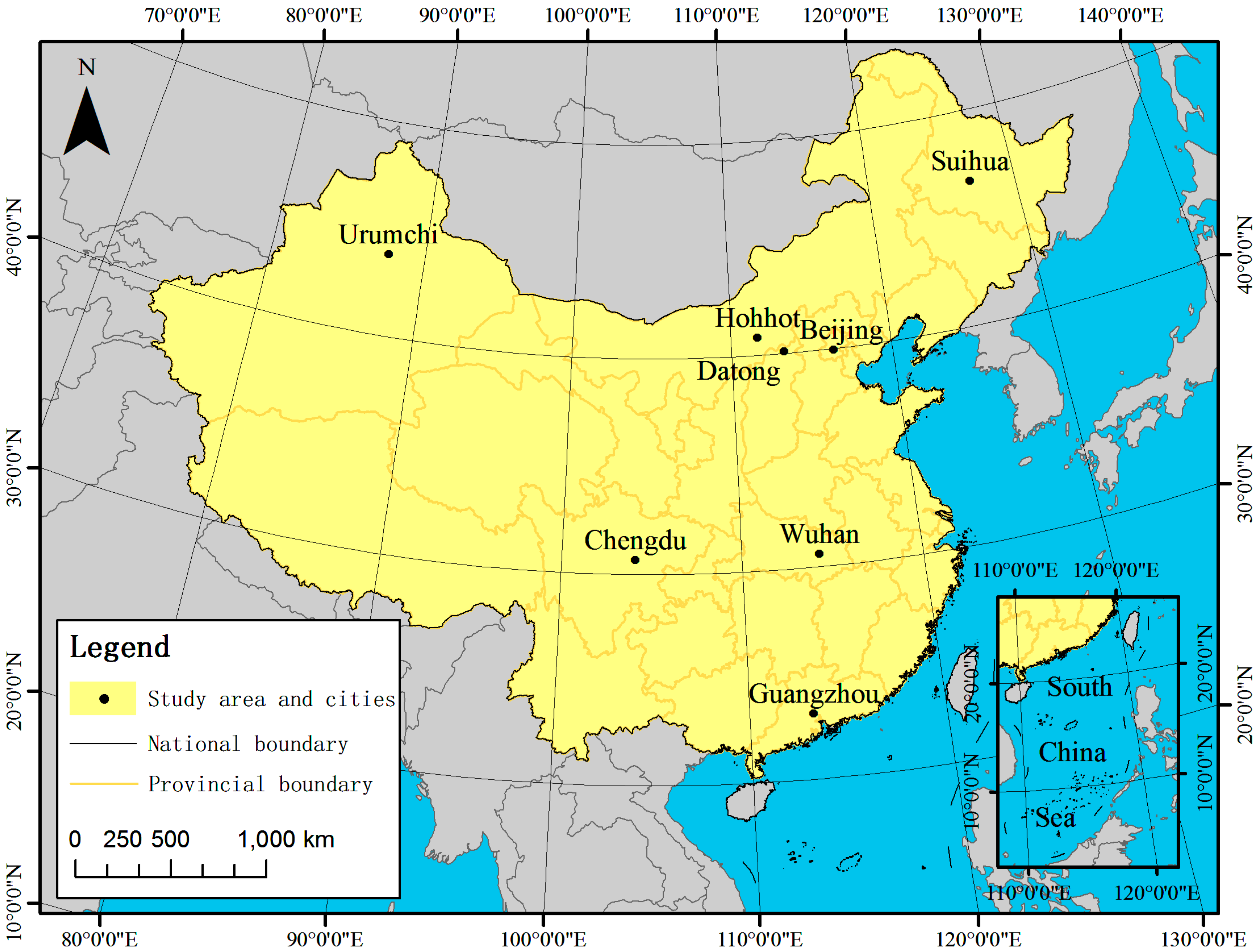
This paper takes mainland China as the case study area, which contains 30 provinces, but excludes the surrounding islands (Figure 1).
Due to the rapid economic and social development, China’s urbanization rate grew rapidly over the past approximately 38 years. Until the end of 2012, more than 0.71 billion Chinese (about 52% of the population) lived in cities [53]. However, the western economy is obviously lagging behind the eastern, and the city-dwelling populations mainly gather in the east. The economic development in China is extremely imbalanced. Besides, China has wide land coverage (approximately 9.6 million km2), and its geographical features vary greatly from region to region. In the southeast coast, the climate is a continental monsoon climate, while it changes into typical inland dry weather in northwest China. Multivariate climate conditions bring out different vegetation characteristics of cities. As annual average precipitation decreases from east to west, vegetation coverage reduces with the same change tendency. Multiple states of the economy and the geographical differences make China an ideal experimental region for estimating the combination of NPP-VIIRS DNB and MODIS NDVI at continental scales.
In addition, eight cities (Urumchi, Suihua, Hohhot, Datong, Beijing, Chengdu, Wuhan and Guangzhou) with different levels of urbanization and different geographical locations are selected as the cases for contrastive analysis in Section 5.
2.3. Data Acquisition and Pre-Processing
Four different sources of data are used for this work: (1) collection 5 MODIS 500 m NDVI data products (MOD13A1) for 2012 [54]; (2) NPP-VIIRS DNB composited data for 2012 [55]; (3) DMSP/OLS NLD acquired by the DMSP satellite F18 for 2012 [56]; and (4) Global Land Cover Mapping at 30 m resolution for 2010 (GLC30-2010) [57]. A brief description of the datasets is listed in Table 1. The input data for classification are the maximum NDVI retrieved from MODIS NDVI products, and the normalized NPP-VIIRS DNB. DMSP/OLS NLD and GLC30-2010 are auxiliary data. The stable DMSP/OLS NLD is employed for filtering NPP-VIIRS DNB, and the GLC30-2010 dataset is used for sample selection. All classification data are reprojected to Albers conical equal area projection by the nearest-neighbor resampling algorithm and resampled into the same spatial resolution of 480 m. Details of the data pre-processing are described as follows.
2.3.1. Generating the Maximum NDVI
NDVI is a graphical indicator that can assess whether the ground surface contains green vegetation. Urban lands also contain vegetation, but with a much lower vegetation coverage rate than the pure vegetation areas such as grassland. There is a negative correlation between NDVI and urban land. Previous research has employed NDVI to estimate the urban extent [42]. However, when a single-date NDVI is used, urban lands are easily confused with some vegetation areas, such as croplands. This is because the NDVI of deciduous vegetation areas varies with the phenological change, while the urban NDVI is relatively stable for several seasons. For example, croplands are mainly covered by plants, having a large NDVI value. After the harvest, however, bare soil will be dominant, and the NDVI values reduce accordingly, which may become the same as that of urban land. Thus, to extract the spectral differences and highlight urban land, the maximum NDVI retrieved from multi-temporal NDVI is employed. The NDVI composite can also remove the impact of cloud contamination.
The MODIS vegetation index product (MOD13A1) provides time- and space-continuous NDVI with 16-day intervals at 500 m spatial resolution. To cover the entire study area, 17 MODIS scenes are required: h23v04, h23v05, h24v04, h24v05, h25v03–h25v06, h26v03–h26v06, h27v04–h27v06, h28v05, and h28v06. For each scene, 23 tiles are available in 2012. Finally, a total number of 391 MODIS tiles are downloaded. The maximum NDVI of each scene is calculated by Equation (1) from all corresponding MODIS NDVI tiles.
where Si is the index of each scene and NDVI1, NDVI2, …, NDVI23 are the MODIS NDVI tiles acquired in 2012.
The NDVI values range from −1 to 1. A positive value, even close to zero, indicates a region covered by vegetation, while a negative value signifies non-vegetated areas, such as water bodies and snow cover. According to the requirements of the classification method, the negative values are removed from the maximum NDVI image. Thus, the NDVI of final maximum image ranges between 0 and 1.
2.3.2. Removing Background Noise and Filtering Extreme Values in NPP-VIIRS DNB
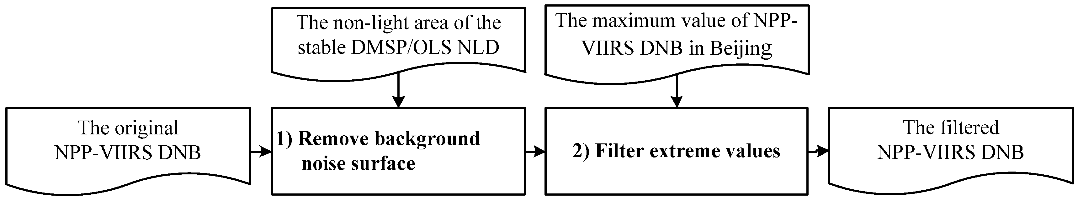
The original nighttime light image was composited by the NPP-VIIRS DNB data with low moonlight during 18–26 April 2012 and 11–23 October 2012. As there exist unstable lights (e.g., fires, gas flares, volcanoes, aurora, etc.) in the original image, it is necessary to remove these background noises and ephemeral lights before use.
A simple method is employed to remove the outliers from the original NPP-VIIRS data [58]. The pre-processing procedure contains two steps (Figure 2). (1) The first step is removing the background noise surface by DMSP/OLS NLD. The stable DMSP/OLS NLD only contains the persistent light (the lights from cities, towns, etc.), and the ephemeral lights (e.g., fires) have been discarded. Thus, the non-light area (DN = 0) of the stable DMSP/OLS NLD is extracted and overlays NPP-VIIRS DNB to mask out the background noise. This step not only retains the stable night light, but also removes many non-urban areas, thus reducing the data process load. (2) The second step is filtering extreme NPP-VIIRS DNB values. The original NPP-VIIRS DNB values range from −0.42 to 3329.31 nW·cm−2·sr−1; however, 90% of the values are smaller than 332.93, and more than 98% of the values are smaller than 63. The extremely high values that are probably caused by lights from some special places such as airports or fires need to be removed. Since the nighttime light has a positive correlation with the economic development level, the maximum value of light brightness should not be larger than that in the most developed city. According to China Statistical Yearbook 2013, Beijing is the most economically advanced city. A maximum value (235.13) from Beijing is chosen to correct the DNB values. All pixel values that are greater than 235.13 are replaced by the mean value of their neighbor pixels. A total of 84 pixels is reassigned in the study area. The filtered NPP-VIIRS DNB values range from 0 to 235.13 nW·cm−2·sr−1.
The classification method used in this paper is not scale invariant. To keep all input data sources (i.e., the maximum NDVI and the NPP-VIIRS DNB data) in the same data range (between 0 and 1), the filtered NPP-VIIRS DNB image is finally normalized with Equation (2):
where DNBni is the normalized value of the ith pixel, DNBi is the original value of the ith pixel and DNBmin and DNBmax are the minimum and maximum values of all pixels, respectively. In addition, to facilitate the classification process, the NPP-VIIRS DNB image is finally split scene by scene according to the MODIS grid.
2.3.3. Aggregating GLC30-2010 from 30 m to 480 m
The world’s first 30 m resolution global land cover dataset (GLC30-2010) consists of 10 first-level classes, namely water bodies, wetland, artificial surfaces, cultivated land, permanent snow/ice, forest, shrubland, grassland, bare land and tundra. An accuracy assessment of the GLC30-2010 dataset was conducted by third-party experts with a total of 159,874 pixel samples [59,60]. The overall accuracy of the GLC30-2010 dataset is 83.5%. In this study, the artificial surfaces (value = 80) were extracted for the training set sampling (Section 2.3.1). The accuracy of artificial surfaces reaches 86.97%.
To maintain a consistent scale, the 30 m spatial resolution artificial surfaces are aggregated to 480 m by a 16 × 16 window based on a majority rule. The value of each aggregated pixel is the area proportion of artificial surfaces. For example, if 143 pixels in a 16 × 16 window are labeled as artificial surfaces, the value of corresponding aggregated pixel will be 0.559 (i.e., 143/(16 × 16)). The aggregated map is an urban area proportion map. According to the definition of “urban extent”, the urban area proportion map can be further classified into two types based on the threshold of 0.5. The values of pixels that are equal to or greater than 0.5 are reassigned to 1, and the other are set to 0, representing urban and non-urban area, respectively. The blocks less than 1 km2 (i.e., 4 pixels) are removed due to the minimum area constraint. The re-classified map is called the GLC30-2010 480 m urban map in this paper.
3. Methods
The processing procedure is summarized in Figure 3. Three key steps are included: (1) sampling training and testing samples from the study area; (2) training classifiers for each scene by the BP neural network-based one-class classification method using the filtered normalized NPP-VIIRS DNB and the maximum NDVI as indicators and predicting the urban extent map of the study area; and (3) assessing the accuracy of the classification results using an independent testing set randomly obtained from the entire study area.
3.1. Sampling
Two datasets are generated: one (training set) is for the classifier’s training, and the other (testing set) is for accuracy assessing of the urban map. They are independent of each other (i.e., testing samples are not included in training sets).
Testing samples (consisting of both positive samples and negative samples) are collected randomly from the entire study area. To ensure the accuracy of testing samples, all labels are manual assigned. Each testing sample is labeled as urban or non-urban using visual interpretation from high spatial resolution images (e.g., Landsat images or Google Earth images) by three professionals, respectively, and the final label is determined by most of the three. A double-blind procedure is employed to reduce the uncertainty and bias during the labeling procedure, i.e., the professionals do not know the classification results. In this study, 20,000 testing samples are randomly selected, including 162 urban samples and 19,838 non-urban samples. The selected testing samples are removed from the study area, and the training samples are then selected from the rest. This step can guarantee that the training and the testing samples are independent datasets.
The training set in this paper only requires urban samples and unlabeled samples, since the classification method employed can train the classifier from positive and unlabeled samples. Unlabeled samples are randomly collected from the background (filtered by the DMSP/OLS NLD non-light area) and do not need to have their class labeled. Urban samples are randomly selected from the urban area. However, even if only one type of positive sample is required to be labeled, manually labeling random samples on a wide geographic scope is time consuming and labor intensive. A semi-artificial sampling strategy is adopted to lessen the workload of labeling during the training set sampling process. First, urban samples are collected from the urban area in the GLC30-2010 480 m urban map, and then, their labels are further validated with high spatial resolution images by visual interpretation. To obtain representative urban samples, the urban patches in the GLC30-2010 480 m urban map are shrunk with one pixel at the edge. This step can also eliminate the uncertainty of pixels on the fringes of cities.
Additionally, the characteristics of cities in different regions are different. For example, the vegetation density in the southeast part of China is usually higher than that in the northwest. The urban samples from the north part may not be able to represent the features of that from the south. Thus, a scene-by-scene basis is employed for training set sampling to avoid biased mapping results. For each scene, 1000 urban samples and 5000 unlabeled samples are randomly selected. The scenes with only a few urban pixels are combined into the neighbor scene. Across the entire mapping region, a total of 7000 urban pixels (about 4.396% of the urban pixels in the shrunken GLC30-2010 480 m urban map) and 35,000 unlabeled pixels (about 0.497% of the total pixels) are selected to construct the training set.
3.2. Training and Predicting
The traditional supervised classification method, the most frequently-used remote sensing method, requires that all land types in an image be completely labeled [61]. However, when the target class is only a specific land cover type, this process becomes labor intensive and time consuming. The one-class classifier is a good choice to solve this problem because it focuses on the target data only.
Different one-class classifiers have been introduced in remote sensing classification. The classic One-Class Support Vector Machine (OCSVM) is one of the most widely-used methods [62]. The core idea of this method is to find the hyperplane that separates the training data from the origin with the maximum margin. OCSVM has been successfully applied in the change detection of one specific class (e.g., fenland and urban extent) [63,64]. Another well-known approach is called the Support Vector Data Description (SVDD) [65]. It is based on the theory of the support vector machine, finding a hypersphere with minimal radius, which encloses all samples of one class and assumes that samples outside this hypersphere do not belong to the class [66]. It has shown promise in the fenland class training [67]. However, the drawback of these SVM-based methods is that too many free parameters are included, which leads to the outcome sensitivity. In addition, the complicated model selection procedures also preclude its adoption [68,69].
A novel one-class classification algorithm called the Present-Unlabeled Learning algorithm (PUL) [70] was introduced into remote sensing image classification [68]. Generally, if both positive data and negative data are available in the training set, traditional binary classifiers (e.g., SVMs) can learn a function to predict the probability of individual samples being positive. However, if only positive and unknown samples are available in the training set, the function cannot be estimated directly by these methods. A lemma was introduced by Elkan and Noto into PUL to train the classifier from only positive and unknown samples.
In this study, the urban class is referred to as the positive class (y = 1), while the non-urban class is referred to as the negative class (y = −1). If the class (urban or non-urban) of a sample x is explicitly known, it will be referred to as labeled (s = 1); otherwise, it will be referred to as unlabeled (s = 0). In this study, only urban samples are labeled. Thus, a labeled sample must be urban, and the probability of a non-urban sample x being labeled is zero, we have
Suppose each urban pixel within the whole image has the same probability of being labeled regardless of its location x, i.e., the probability that an urban sample is labeled is a constant c, we have
The constant c indicates the level that positive data are detected or labeled in the samples. For example, suppose that a study area contains 50 positive samples and 50 negative samples. c = 1 means all the positive samples are labeled; c = 0.5 means approximately 25 positive samples are detected, resulting in 25 labeled data and 75 unlabeled data.
The target of a binary classifier is estimating a function f(x) = p(y = 1|x) from the finite training data. With a random selected training set that satisfies Equations (3) and (4), we can train a function g(x) = p(s = 1|x) in PUL, we have
Substituting f(x) = p(y = 1|x) and c = p(s = 1|y = 1), which we defined, we have
which is to say that the difference between the classifier f(x) and g(x) is a constant c. If we estimate the constant, the desired classifier f(x) can be obtained.
The constant c can be estimated from a validation set. Suppose a validation set V is randomly drawn from the original training set; P is the labeled samples in V, hence positive (urban). For all pixels in P (i.e., x ∈ P), there is p(y = 1|x) = 1 and p(y = −1|x) = 0. Therefore,
which is to say that the constant c can be estimated by any g(x) from the subset P, if g(x) = p(s = 1|x). To obtain a more reliable estimator of the constant c, the average values of g(x) (x ∈ P) are employed, as shown in Equation (8):
where n is the cardinality of P.
In summary, to evaluate the probability of a pixel being urban area, two steps are required in this paper. First, the function g(x) is trained by only urban pixels and unknown pixels, which satisfied Equations (3) and (4), and estimated the constant c from Equation (8). Secondly, the desired classifier f(x) is obtained by calibrating g(x) with c on the basis of Equation (6).
It is worth noting that PUL is not a specific classifier, but a general framework for classifier learning. In this study, the Back Propagation (BP) neural network is used as the classifier. It has been proven that PUL is insensitive to outliers and parameters [71]. PUL is able to predict the probability of presence without negative data. It simply requires a small set of positive data and a large set of unlabeled data to help train a classifier and estimate the posterior probabilities of the target class, which can reduce the work in collecting samples and hence accelerate classification efficiency. This makes PUL an ideal method in regional urban extent mapping. More details of the principle and process of its deduction can be found in the paper [70,71,72].
3.3. Accessing Accuracy
To quantify the performance of built-up urban areas extracted by our classification scheme, the conventional approach is employed, i.e., comparing our classified map with an independent, random sample of “ground truth” points [73].
The overall accuracy (OA) is the commonly-used index for accuracy assessment. However, when there is class imbalance (i.e., the non-urban samples far outnumbers the urban samples), the overall accuracy is not an appropriate evaluation criterion [74,75]. It is often biased towards the majority classes, ignoring the minority classes. To avoid the influence of the relatively small portion of urban area compared with non-urban area on the total accuracy, we employ another three indexes: the producer’s accuracy, the user’s accuracy and the kappa coefficient as performance evaluation measures. The producer’s accuracy evaluates the omission error, which indicates the probability that a reference urban pixel will be correctly identified. The user’s accuracy measures the commission error, indicating the probability that a classified urban pixel is truly urban. The kappa coefficient combining both types of errors can provide a more comprehensive assessment [76]. Kappa measures the agreement between our results and the ground truth samples. The closer that the kappa value is to 1, the higher the agreement is [77,78,79]. A confusion matrix is established to perform the accuracy assessment. The formulas of overall accuracy and the kappa coefficient are as follows:
where N is the total number of pixels in the testing set, xkk is the diagonal of the classification confusion matrix, xk+ is the total number of pixels of the k class and x+k is the total number of pixels that are classified into the k class.
4. Results
4.1. Urban Land Classification Accuracy on the Pixel Level
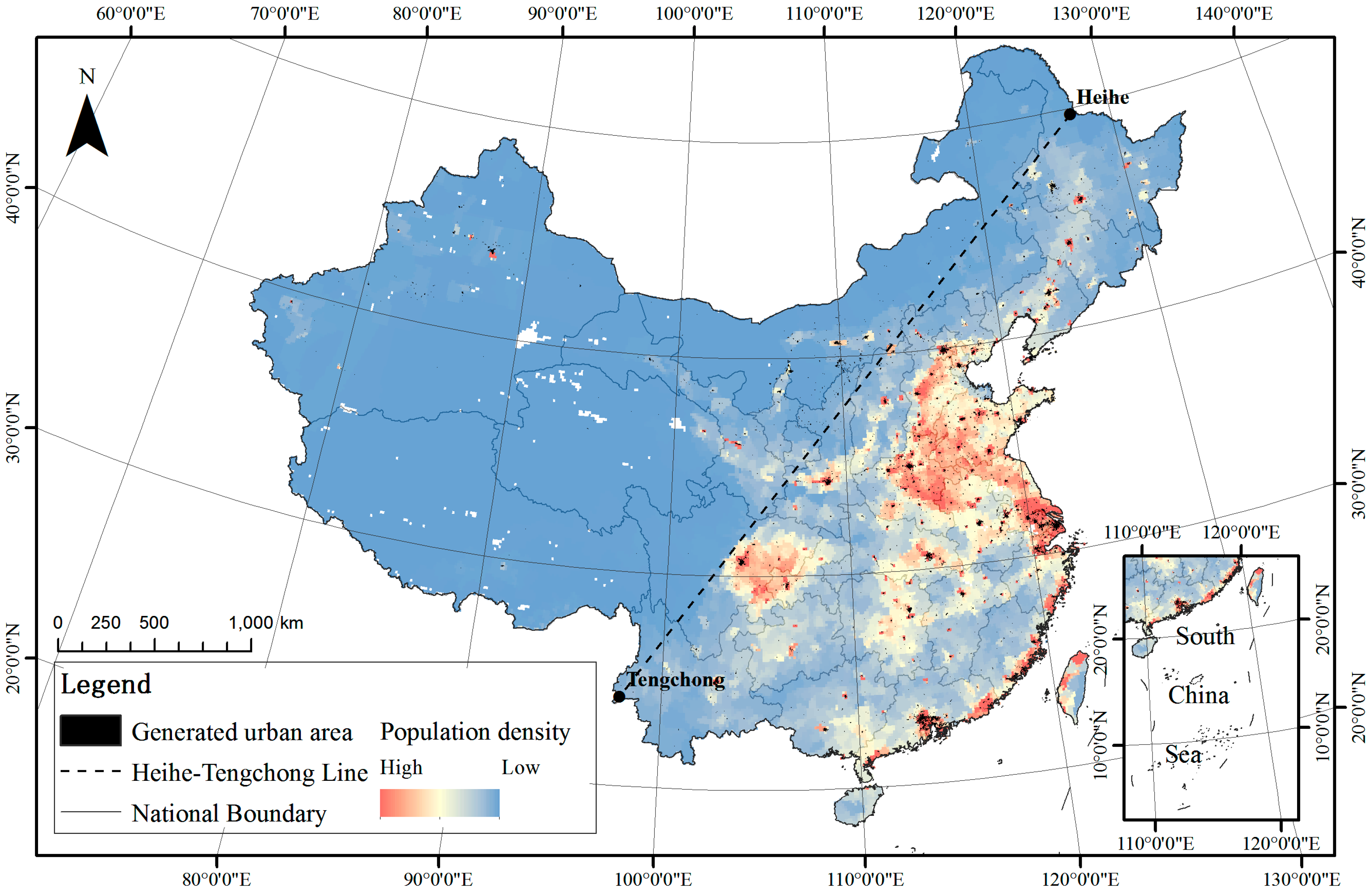
The final urban extent map obtained by the proposed classification scheme is shown in Figure 4. The predicted urban area is 68,023.75 square kilometers (295,242 pixels, approximately 0.71% of the total area). The urban blocks are not evenly distributed, mainly in the north of China and the southeast coastal areas and rarely in the west parts. If we divide the study area into two roughly equal parts by the Heihe-Tengchong Line [80], 87.9% of the urbanized areas are contained to the east of the line, which has the same tendency as the population density. The eastern urban coverage rate is 1.7%, higher than the average.
Accuracy assessment using randomly selected urban and non-urban samples shows that the accuracy of the obtained urban map is high. The total accuracy for urban area detection is 99.76%, and the kappa coefficient is 0.842 (Table 2). The user accuracy for urban areas is 89.58%, indicating that only a very small number of non-urban areas are misclassified as urban. In terms of the producer’s accuracy of urban areas, about 80% of the reference urban areas are successfully identified.
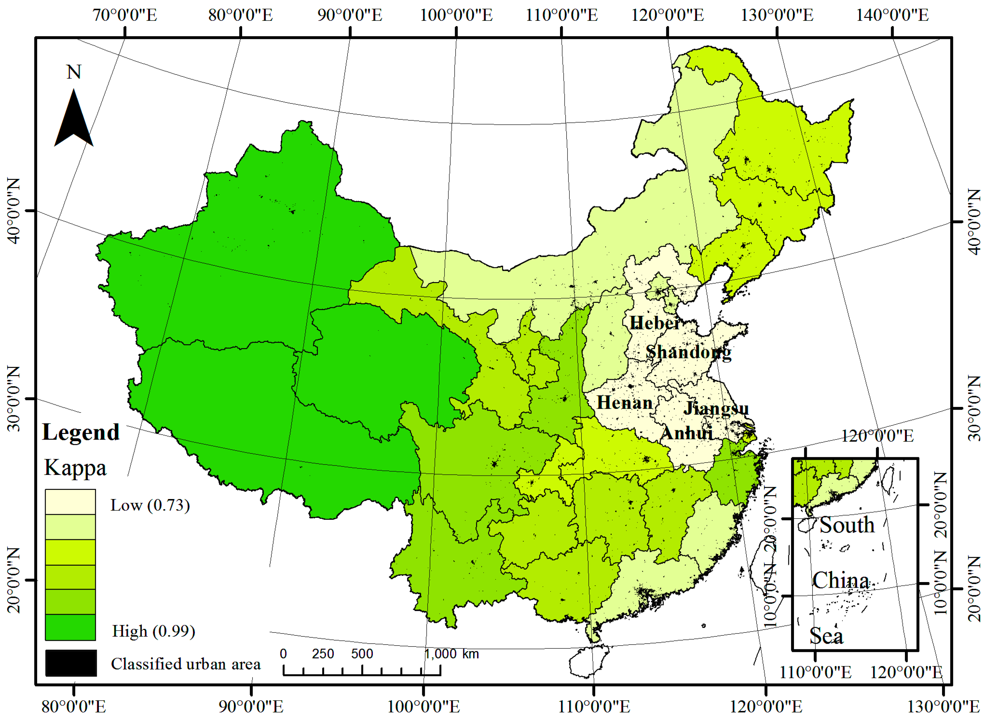
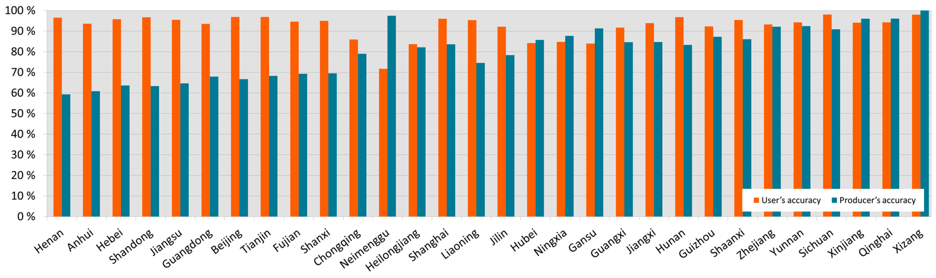
To better understand the classification results, accuracy assessment was also conducted on sub-regions. The study area was divided into 30 sub-regions according to the provincial administrative boundaries. To assure the spread of urban samples in each validation set, at least 50 urban samples were collected in each sub-region. Due to the imbalanced composition of urban and non-urban features, area adjustment was conducted for each accuracy assessment. The number of non-urban samples was based on its coverage rate. All collected samples were manually validated with Landsat images or Google Earth images by visual interpretation. The OA, kappa coefficient, user’s and producer’s accuracy of each sub-region were calculated. The sub-region accuracies are similar to that obtained from the entire study area. The provincial overall accuracies are all greater than 90%, averaging 99.34%. The value of the kappa coefficient varies from 0.73 to 0.99, with an average of 0.848. The kappa coefficients are divided into six classes by equal intervals (Figure 5). The western have a higher kappa than the eastern parts, especially the five provinces with the lowest kappa (0.730, 0.734, 0.761, 0.761 and 0.766 for Henan, Anhui, Hebei, Shandong and Jiangsu, respectively). Figure 6 demonstrates the user’s and producer’s accuracy of each province, which represents the commission errors and the omission errors, respectively. For most provinces, the user’s accuracies (92.49% on average) are higher than the producer’s accuracies (an average of 80.23%), which also remain broadly in line with the results of the whole map.
The commission errors of this map mainly occurred in cultivated land and water areas. If we remove water bodies by water masks from the final map, the overall accuracy will rise to 99.80%, and the kappa coefficient will reach 0.865. It can be said that most of the classified urban areas are correctly classified. The omission errors mainly occurred in cultivated land. The area of some tribal non-city regions is beyond the minimum requirement of the definition of urban extent (i.e., 1 km2), but the factors such as low population intensity and less human activity at night have a negative influence on the nighttime light data. When integrating nightlight data for classification, they may be omitted. That is also the factor contributing to the relatively low kappa coefficient for the five provinces (Henan, Anhui, Hebei, Shandong and Jiangsu). The producer’s accuracies of the four provinces are much lower than their user’s accuracies (Figure 6). An average of 38% of the urban blocks in this area is omitted. That is because this area is the major agricultural region in China (the North China Plain), where a large number of villages and towns are located. The omissions of the small “urban blocks” reduce the classification accuracy.
In general, the classification results are satisfied. On the pixel level, the proposed classification scheme has successfully identified most urban extent and with a high classification accuracy.
4.2. Urban Land Classification Accuracy on the City Level
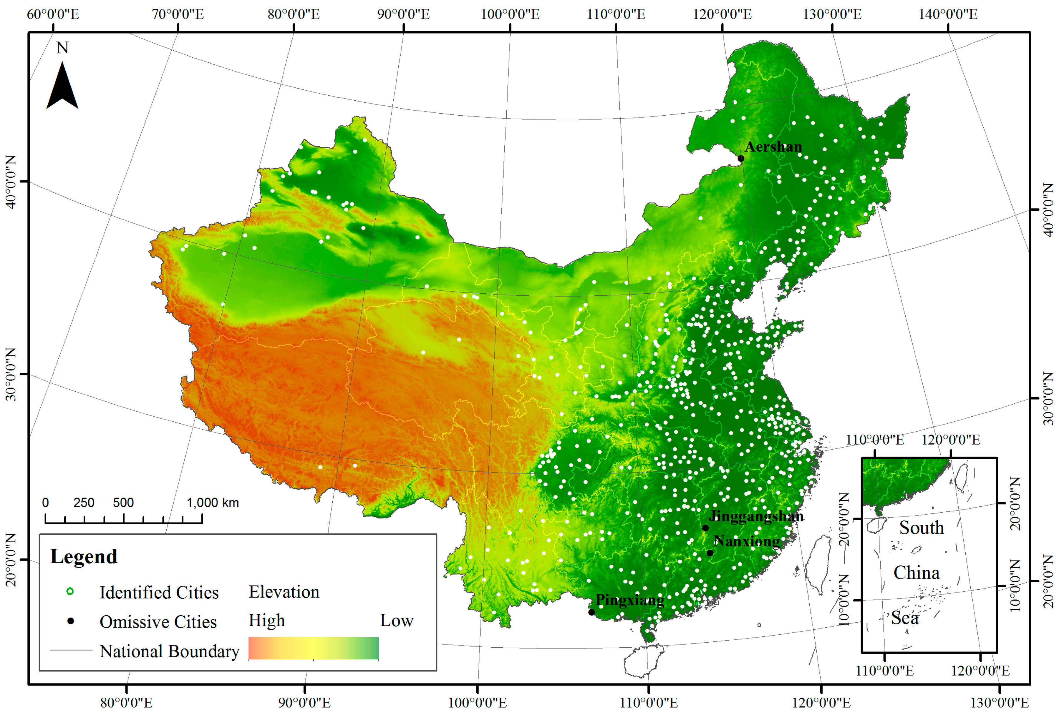
To assess the classification accuracy on the city level, 647 cities and counties are selected based on China City Statistical Yearbook 2013. Cities are divided into four groups by administrative levels: municipality directly under the central government, vice-provincial city, prefecture-level city and county-level city (Table 3). The locations of the administrative department of each city are shown in Figure 7, represented by points.
The accuracy is high, reaching 99.38%. The classification scheme successfully mapped all of the municipalities directly under the central government, vice-provincial cities and prefecture-level cities. Only four county-level cities are omitted (Aershan, Jinggangshan, Nanxiong and Pingxiang).
From the spatial distribution perspective, the omissions are distributed mainly in the mountainous regions, and most land areas of the four cities are covered by farmland, grassland or mountain land; the urban blocks are relatively small. For example, Nanxiong, located in the northeastern part of Guangdong Province, is surrounded by the Dayu Mountains; over 80% of the areas of Pingxiang are covered by hilly regions, and the forest coverage of Jinggangshan reaches up to 81.2%. Due to the high coverage of vegetation, the NDVI values in these cities may be relatively higher than other cities. In addition, their population densities are relatively low. For instance, Aershan, an omission case located in the northeastern part of China, only contains a population of 48 thousand, but its land area is 7408.7 km2. Accordingly, the DNB values within the cities, as a signal of human activity, are much lower than a typical city, which may cause the omission errors.
5. Discussion
5.1. Comparative Analysis of Urban Extent under Different Nighttime Light Data
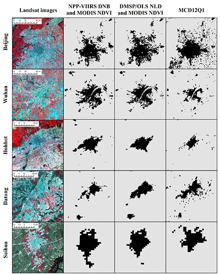
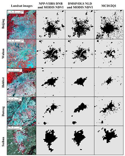
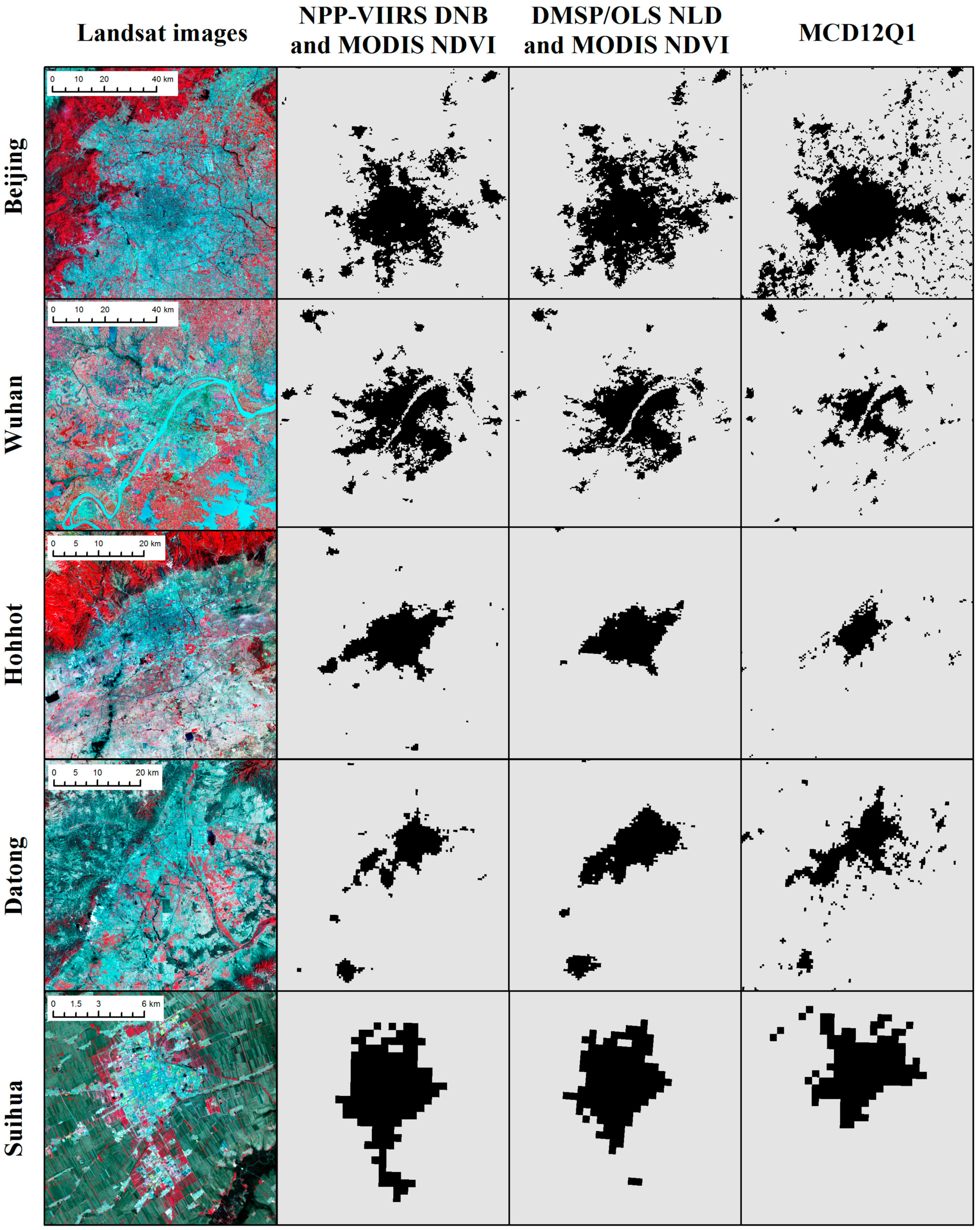
Previous studies have recommended the NPP-VIIRS DNB for extracting urban extent at regional and continental scales [24,31]. The wider radiometric range and finer spatial resolution of NPP-VIIRS DNB provide an opportunity to obtain more detailed information about the urban extent. Thus, for contrastive analysis of the classification performance of different nighttime light data under the proposed classification scheme, another urban land map of the study area in 2012 was generated by DMSP/OLS nighttime light data and the maximum MODIS NDVI (Column 3, Figure 8). The maximum MODIS NDVI images, the training samples and the classification method (i.e., the PUL algorithm) are the same as used in this paper (Column 2, Figure 8). The only difference for the two maps is the source of the nighttime light data. In addition, public land cover datasets (MCD12Q1 in MODIS products [81]) are also employed, and the urban and built-up layer is extracted for comparison (Column 4, Figure 8). All maps demonstrate the situation of urban extent in 2012. Landsat images used as the ground truth are collected between October 2012 and August 2013 for the best display effect (Column 1, Figure 8).
Five cities, Beijing, Wuhan, Hohhot, Datong and Suihua, at different levels and scales were chosen as the cases of interest. Beijing is the biggest megacity in China with the largest population and Gross Domestic Product (GDP). Wuhan is a megacity located in Central China. Hohhot, Datong and Suihua are located in North China. The locations of the cities are shown in Figure 1. For each city, the urban omission rates of different productions are also calculated (Table 4). The same reference samples are used in each city.
Compared with MCD12Q1, NPP-VIIRS DNB and MODIS NDVI (referred to as “Group 1” below) have a better performance on the urban extent. Although the omission rate of Beijing generated by Group 1 (39.39%) is relatively higher than the other two maps, 27.27% for the map generated by DMSP/OLS NLD and MODIS NDVI (referred to as “Group 2” below) and 28.28% for MCD12Q1, its urban boundaries are more consistent with the ground truth. The urban extent in MCD12Q1 is smaller than that in the former two maps, and it is also inconsistent with that shown in the Landsat images. Many urban pixels especially those located in the urban fringe are omitted in MCD12Q1. The omission rate of MCD12Q1 is much higher than that of the other two productions, topping out at 57.14% in Suihua. In addition, the “salt and pepper” effect is relatively evident in MCD12Q1, such as Beijing. Through manual validation, it is found that many tiny urban blocks around main cities in MCD12Q1 are commission errors; cultivated lands or bare lands are frequently misclassified as urban lands.
For the two urban maps generated by different nightlight data, the difference is mainly in small urban blocks. The small urban blocks far away from city centers are often missed by Group 2. This phenomenon exists obviously in small cities. For example, in Hohhot, compared with the urban map generated by Group 1, surrounding small urban blocks are obviously lost by Group 2. That is why the omission rates of Group 1 are still in single digits, such as Suihua with only 8.57%, while those of Group 2 are far more than that, reaching 37.14%. The small urban blocks near city centers are merged into the large blocks. Some details of urban pattern are lost in the map generated by Group 2, such as Datong.
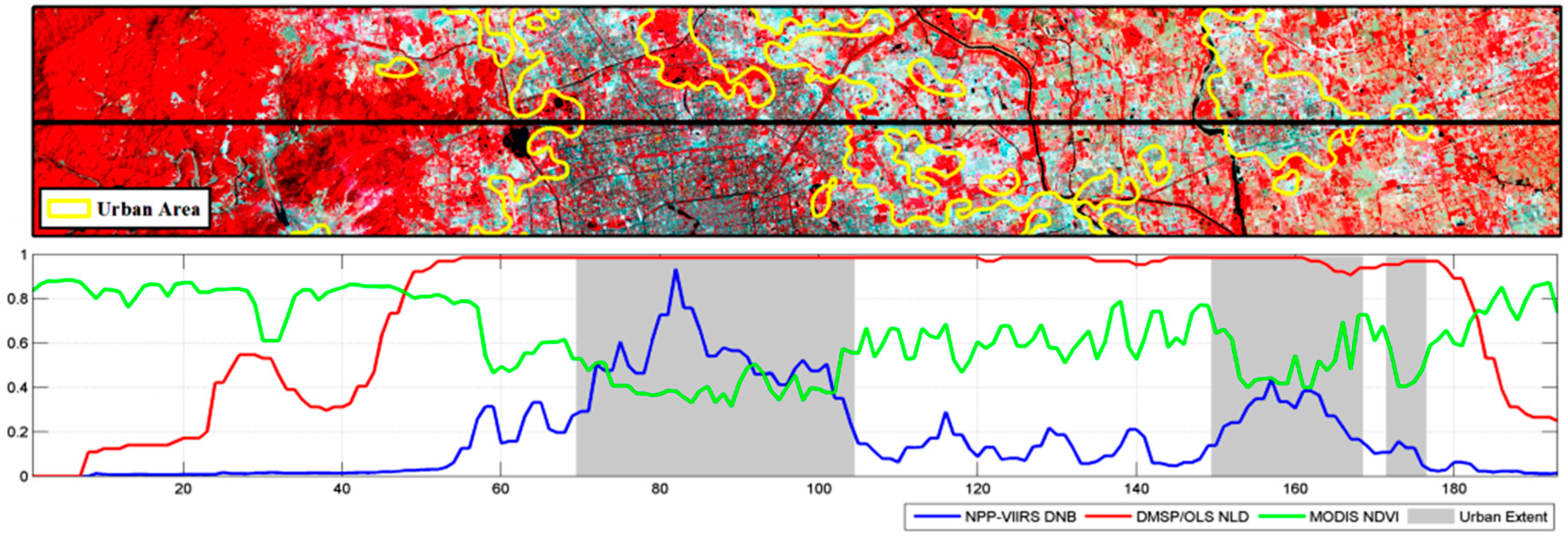
In general, NPP-VIIRS DNB has a better performance on detecting low light area, such as small urban blocks and the edge of cities. It can be seen from Figure 9 that when the value of NPP-VIIRS DNB starts to rise from the bottom, DMSP/OLS NLD is already saturated. Although NDVI makes up some detail losses, the high nighttime light values preclude the separation of the non-urban areas. This makes the small urban blocks close to city centers be merged into the large urban blocks, resulting in detail losses and overestimation. In addition, the DMSP/OLS NLD is limited at detecting low light. Isolated small urban blocks with faint light are easily ignored, causing omission errors.
5.2. Case Analysis: Performance of Combining NPP-VIIRS DNB and MODIS NDVI
Different remotely-sensed data have their own characteristics, and combined use of them could provide more information than individually [42]. To evaluate the performance of combining NPP-VIIRS DNB and MODIS NDVI, we analyzed the distribution frequencies of the maximum NDVI calculated for the entire year and the NPP-VIIRS DNB value of four frequently-confused land cover types, including cultivated land, water bodies, artificial surfaces and bare land. The definitions of the four land cover types refer to those in GLC30-2010 dataset, since the training samples in this paper are collected mainly based on this dataset. The accuracy of cultivated land, water bodies, artificial surfaces and bare land in GLC 30-2010 is 82.76%, 84.70%, 86.70% and 81.76%, respectively.
Five cities (Beijing, Wuhan, Guangzhou, Chengdu and Urumchi) distributed across various geographies in China are employed as the cases (Figure 1). To maintain the consistent spatial resolution, pixels are aggregated to 480 m based on the majority rule. All pixels of the four land cover types in these cities are counted.
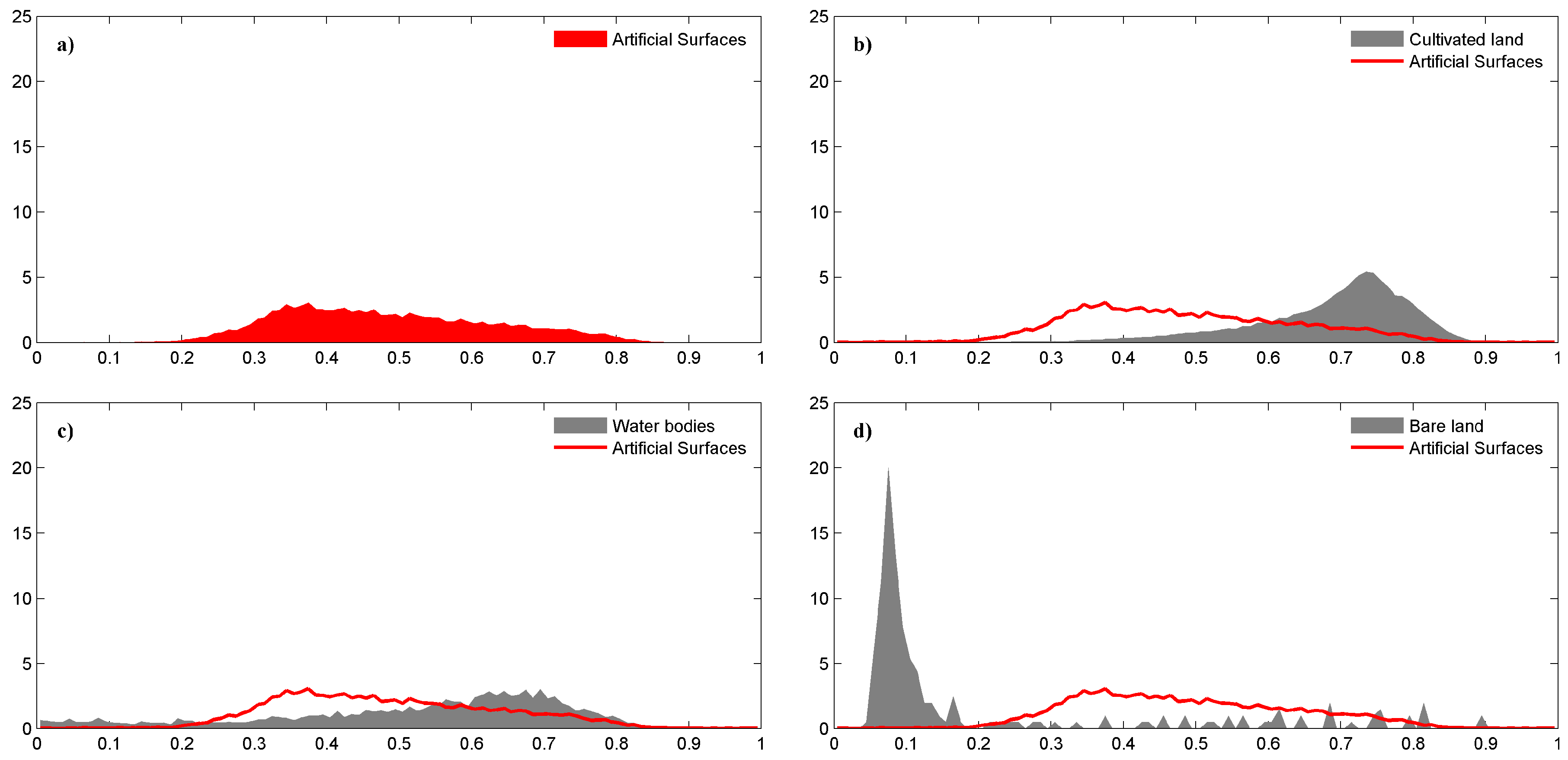
The distribution frequencies of the NDVI value of the four land cover types are shown in Figure 10. It can be seen that artificial surfaces have NDVI values between 0.3 and 0.8 (Figure 10a). Cultivated land shows prominent vegetation characteristic. The NDVI is mainly distributed between 0.6 and 0.9; only a small part is distributed among 0.4 to 0.5. A value below 0.4 is rarely observed (Figure 10b). NDVI values of water bodies have a wide distribution, ranging from 0.1 to 0.9 (Figure 10c), and NDVI values of bare land are mainly below 0.2 (Figure 10d).
Although the NDVI distribution trends of these four land covers are different, there is still significant overlap. Many pixels of cultivated land have a similar NDVI value to that of artificial surfaces, especially between 0.5 and 0.7. That is, during this interval, little difference exists between cultivated land and artificial surfaces. The NDVI value distribution areas of bare land and water bodies are also overlapped with that of artificial surfaces. However, the overlap area of bare land is small, and the pixels of water bodies are few in number. Bare land and water bodies are not the main confused land covers. If only using NDVI as the factor for classification, artificial surfaces may result in many misclassification errors.
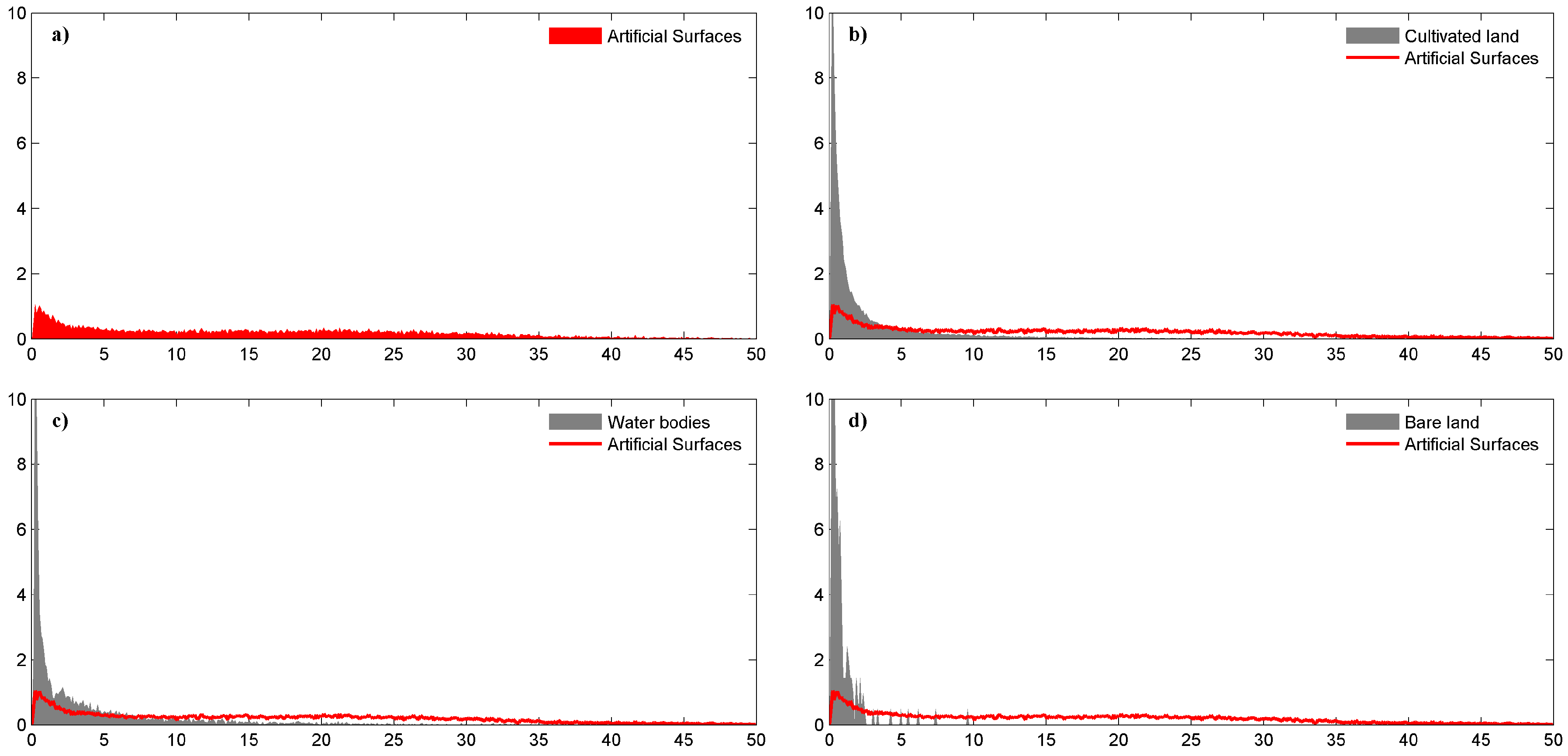
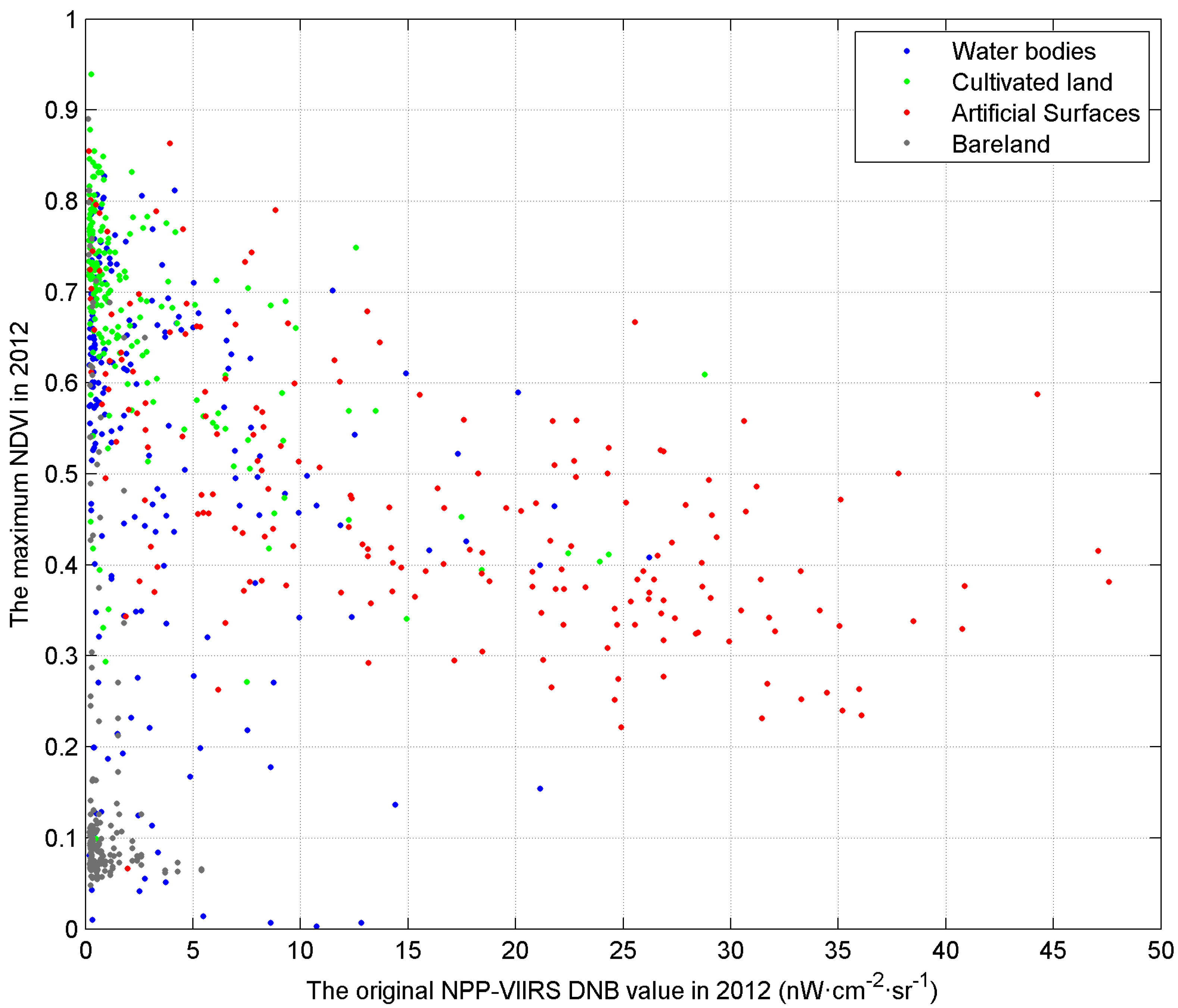
Figure 11 demonstrates the distribution frequencies of the NPP-VIIRS DNB value of the four land cover types. Most DNB values of cultivated land, water bodies and bare land are distributed below five, while those of artificial surfaces are relatively evenly distributed. However, there are still some low light areas (DNB < 5) existing in artificial surfaces, resulting in confusion.
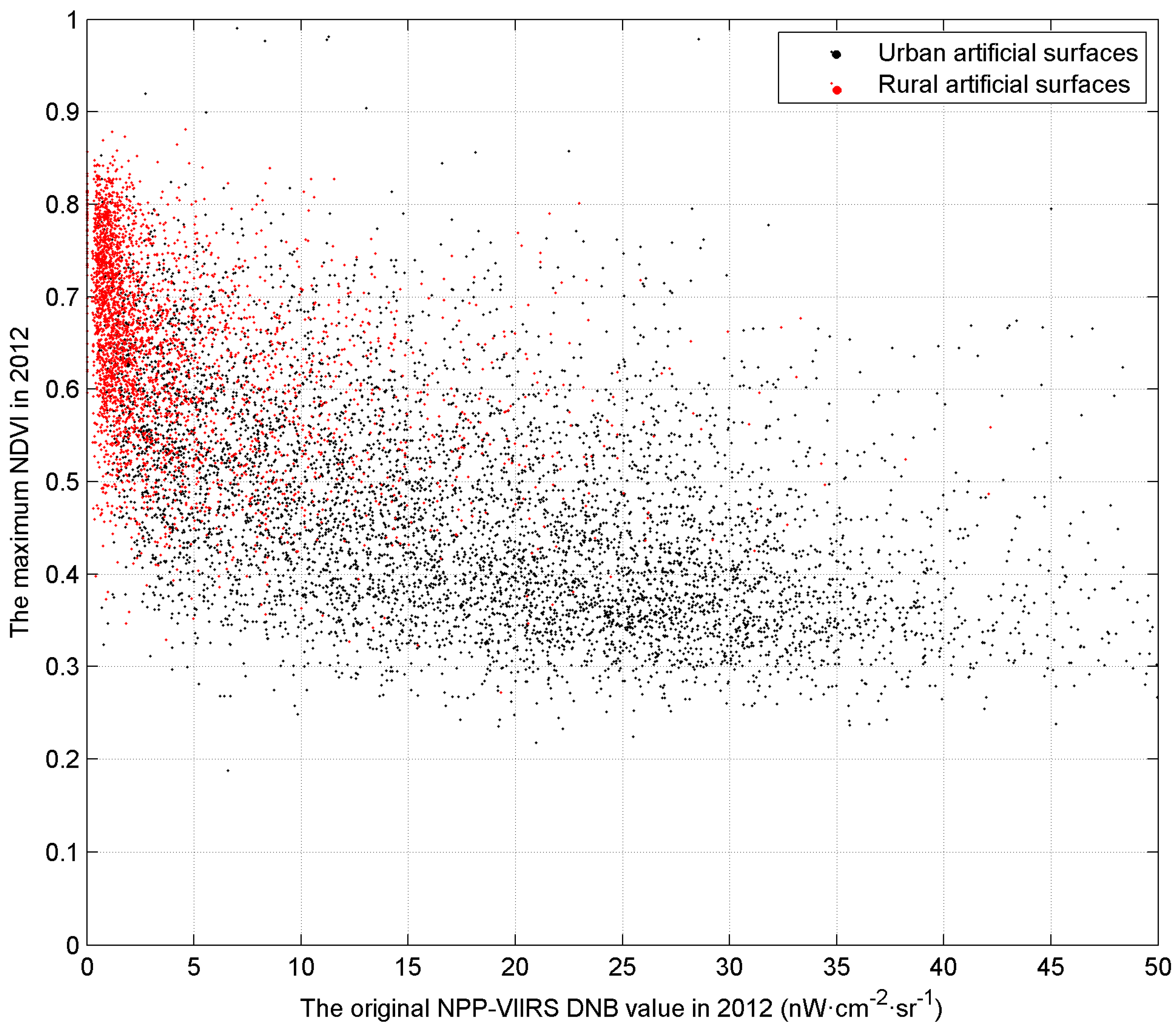
It is a bit difficult to separate these land cover types based on one single type of data. Figure 12 demonstrates the simultaneous use of NPP-VIIRS DNB and the maximum MODIS NDVI (200 random samples). It can be seen that most features can be distinguished by the two-dimensional feature. Almost all of the bare land is separated from artificial surfaces. Only a small part of water bodies and cultivated land with relatively high nightlight values is mixed in the main part of artificial surfaces, which may cause commission errors. It is important to note the low light parts. Because the low nighttime light is not the typical urban feature, artificial surfaces in this part are frequently omitted during the classification. This is also the main error of our classification results. For a further understanding of the artificial surfaces, we classified artificial surfaces into two types: urban artificial surfaces and rural artificial surfaces. If a pixel is surrounded mainly by cultivated land, it will be considered as a rural artificial surface; otherwise, it is an urban artificial surface. As seen in Figure 13, urban artificial surfaces have relatively higher nightlight values and lower NDVI values. Conversely, the artificial surfaces with low nightlight and high NDVI are mainly located in rural areas. That is, the combination of NPP-VIIRS DNB and MODIS NDVI can well distinguish urban artificial surfaces, but is limited in identifying rural artificial surfaces. It could also explain why the omission errors of our map mostly occurred in rural areas.
5.3. Reliability Analysis
Several indexes have been proposed to combine the advantages of both NPP-VIIRS DNB and MODIS NDVI features [31,48]. It has been proven that these indexes are effective on large-scale urban extent extraction. Different from the indexes, the classification method employed in this paper, i.e., PUL, combines NPP-VIIRS DNB with MODIS NDVI in a nonlinear way. It is necessary to evaluate the reliability of this nonparametric fusion approach.
For contrastive analysis on the reliability, an impervious surface index distribution mapping method, Large-scale Impervious Surface Index (LISI) [31], was introduced. LISI was calculated under the same input data as those used by PUL. The formula of LISI is shown as follows:
where NDVIMAX is the maximum NDVI from multi-temporal NDVI images and DNBnor is normalized VIIRS-DNB data ranging between zero and one. Since NDVIMAX is negatively related to ISA while DNBnor has a positive relation, a lower NDVI and a higher DNB represent a higher probability of ISA, i.e., LISI.
To visualize the difference of probability distribution between LISI and PUL, the standard deviation is calculated with a 3 × 3 window. The value of the center pixel is replaced with the standard deviation of the neighboring pixels. A higher standard deviation represents a larger variation of the probability values.
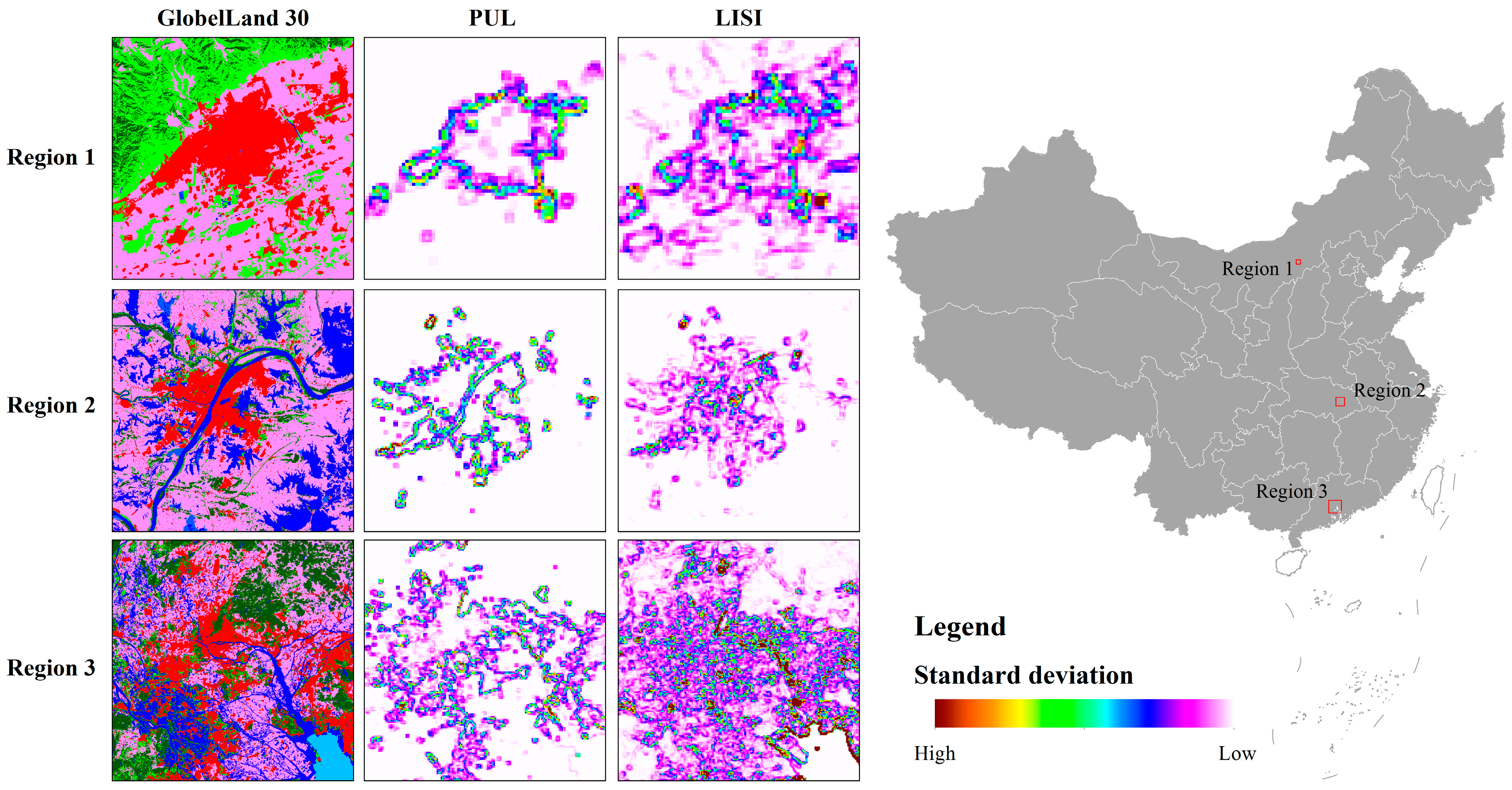
Three regions with various economic conditions and geographic environments were selected as the test area (Figure 14), located in northern China (Region 1), central China (Region 2) and southern China (Region 3). First, the probability distribution in test areas was calculated with LISI and PUL, respectively, and then, based on the output probability map, the standard deviations were further calculated.
As shown in Figure 14, the spatial distribution of the standard deviation calculated by PUL presents a regular shape, and it almost surrounds the urban areas, which means the probabilities on the urban fringe calculated by PUL display an obvious change. The probabilities of inner cities are higher than in the outside. In contrast, the standard deviation calculated by LISI shows more details of inner cities. The probabilities decrease from high values in core urban areas to low values in rural areas, and the urban boundary is vague. Thus, when mapping urban areas into a binary image, PUL is more practical and effective, since the threshold of the urban boundary is much easier to set.
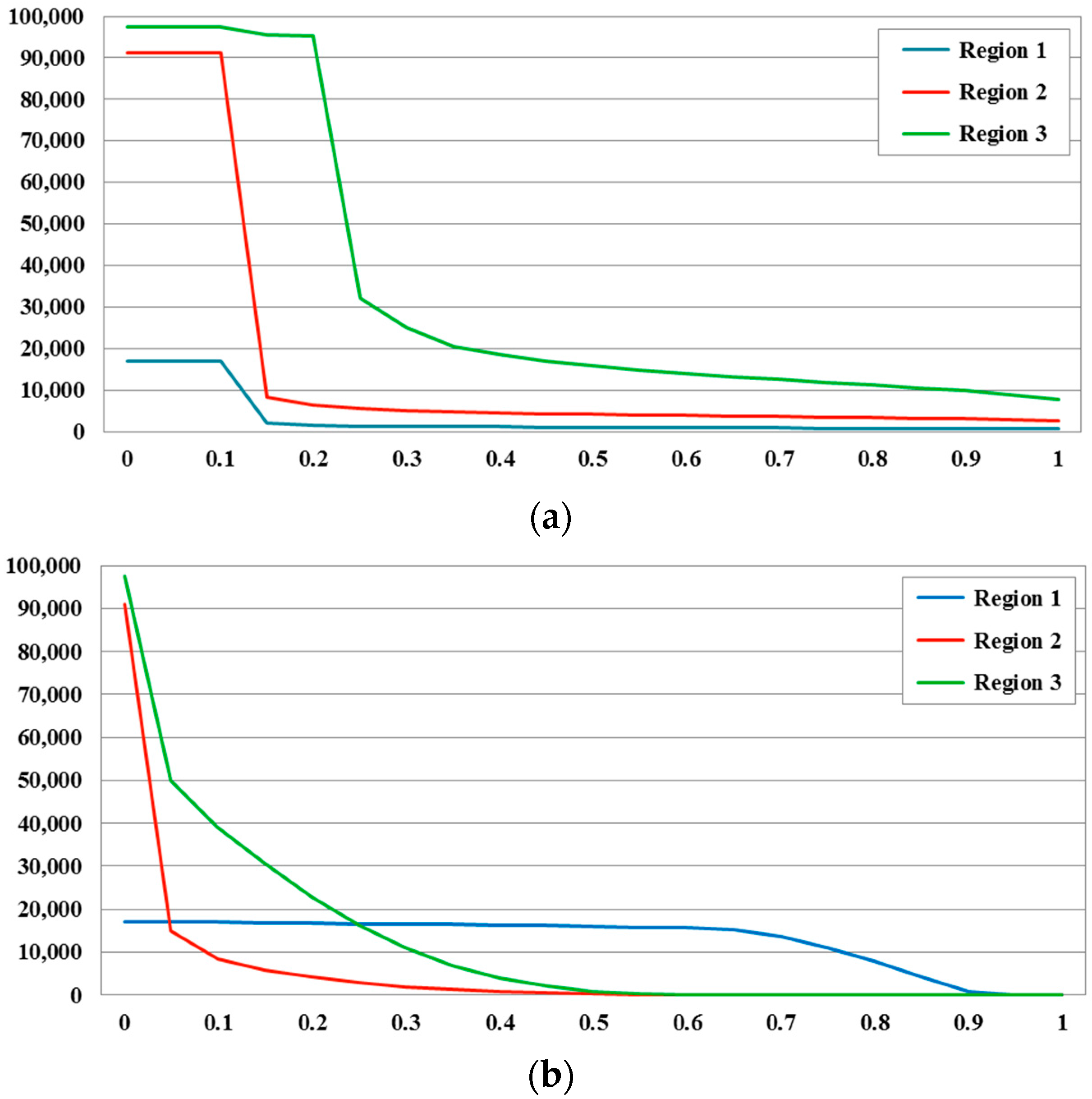
To prove this, we calculate the urban pixel count under different threshold in steps of 0.05 (Figure 15). It can be seen from the line charts that the urban pixels of the three regions calculated by PUL are rapidly converged in a small range (within 0.1), while the reduction speed of the urban pixels in LISI is slower (about 0.1 to 0.3). The slow convergence makes it difficult to select a suitable threshold for LISI. In addition, in LISI, the convergence rates of different regions are different, e.g., when the threshold is 0.2, the urban pixels count in Region 2 tends to converge; however, it is not converged in Region 1, only until 0.7. That is, when using LISI, different thresholds are required for different regions. By contrast, the PUL method is insensitive to the threshold and has good robustness (Table 5). Thus, for regional urban extent mapping, PUL is a more appropriate choice.
6. Conclusions
This study presented an urban-mapping scheme for large-scale mapping. We employed a BP neural network-based one-class classification method (the PUL algorithm) to map the urban extents of China in 2012 by using NPP-VIIRS DNB and MODIS NDVI as variables. The kappa of the obtained binary urban map reached 0.842, which shows the effectiveness of this classification scheme. The combined use of MODIS NDVI and NPP-VIIRS DNB can significantly help to separate urban blocks from the background and reduces errors caused by confusing land covers (e.g., bare land, cultivated land and waterbodies). Compared with DMSP/OLS NLD, NPP-VIIRS DNB has a better performance for detecting underdeveloped towns and suburban areas with low light brightness of nighttime light data, supplying more detailed information about the urban extent. In addition, the classification method (PUL) can significantly reduce the effort needed in assigning labels to train samples and is robust to the threshold, showing great potential to map urban extent at a large scale. Although our result is lacking for the rural regions, the urban extent estimated from our classification scheme is of high accuracy. In the future, we will further improve the procedure for rural artificial surfaces and produce a highly accurate global-scale urban map.
Acknowledgments
This study is supported by the National Key Research & Development (R&D) Plan of China (Project Number 2016YFB0502304). The authors would like to thank the National Geomatics Center of China (NGCC) and Jun Chen for the provision of the GlobeLand30-2010 dataset; Wangxing Lu, Kejun Huang and Wenkai Chen for their help with manual validation; and the anonymous reviewers for their constructive comments and suggestions, which helped improve our paper.
Author Contributions
Run Wang and Bo Wan designed the experiment; Run Wang and Bo Wan collected the required data; Run Wang and Maosheng Hu performed the experiment; Run Wang, Bo Wan, Qinghua Guo and Maosheng Hu conducted the analysis of the results; and Run Wang, Bo Wan, Qinghua Guo and Shunping Zhou contributed towards writing the manuscript.
Conflicts of Interest
The authors declare no conflict of interest.
References
- Seto, K.C.; Fragkias, M.; Guneralp, B.; Reilly, M.K. A meta-analysis of global urban land expansion. PLoS ONE 2011, 6, e23777. [Google Scholar] [CrossRef] [PubMed]
- Small, C. High spatial resolution spectral mixture analysis of urban reflectance. Remote Sens. Environ. 2003, 88, 170–186. [Google Scholar] [CrossRef]
- Grimm, N.B.; Faeth, S.H.; Golubiewski, N.E.; Redman, C.L.; Wu, J.; Bai, X.; Briggs, J.M. Global change and the ecology of cities. Science 2008, 319, 756–760. [Google Scholar] [CrossRef] [PubMed]
- Seto, K.C.; Güneralp, B.; Hutyra, L.R. Global forecasts of urban expansion to 2030 and direct impacts on biodiversity and carbon pools. Proc. Natl. Acad. Sci. USA 2012, 109, 16083–16088. [Google Scholar] [CrossRef] [PubMed]
- Kalnay, E.; Cai, M. Impact of urbanization and land-use change on climate. Nature 2003, 423, 528–531. [Google Scholar] [CrossRef] [PubMed]
- Karl, T.R.; Trenberth, K.E. Modern global climate change. Science 2003, 302, 1719–1723. [Google Scholar] [CrossRef] [PubMed]
- Chen, X.L.; Zhao, H.M.; Li, P.X.; Yin, Z.Y. Remote sensing image-based analysis of the relationship between urban heat island and land use/cover changes. Remote Sens. Environ. 2006, 104, 133–146. [Google Scholar] [CrossRef]
- Shao, M.; Tang, X.; Zhang, Y.; Li, W. City clusters in China: Air and surface water pollution. Front. Ecol. Environ. 2008, 4, 353–361. [Google Scholar] [CrossRef]
- Kaufmann, R.K.; Seto, K.C.; Schneider, A.; Liu, Z.; Zhou, L.; Wang, W. Climate response to rapid urban growth: Evidence of a human-induced precipitation deficit. J. Clim. 2007, 20, 2299–2306. [Google Scholar] [CrossRef]
- Mills, G. Cities as agents of global change. Int. J. Climatol. 2007, 27, 1849–1857. [Google Scholar] [CrossRef]
- Jin, K.; Wang, F.; Chen, D.; Jiao, Q.; Xia, L.; Fleskens, L.; Mu, X. Assessment of urban effect on observed warming trends during 1955–2012 over China: A case of 45 cities. Clim. Chang. 2015, 132, 631–643. [Google Scholar] [CrossRef]
- Schneider, A.; Friedl, M.A.; Potere, D. Mapping global urban areas using MODIS 500-m data: New methods and datasets based on ‘urban ecoregions’. Remote Sens. Environ. 2010, 114, 1733–1746. [Google Scholar] [CrossRef]
- Gong, P.; Wang, J.; Yu, L.; Zhao, Y.; Zhao, Y.; Liang, L.; Niu, Z.; Huang, X.; Fu, H.; Liu, S. Finer resolution observation and monitoring of global land cover: First mapping results with Landsat TM and ETM+ data. Int. J. Remote Sens. 2013, 34, 2607–2654. [Google Scholar] [CrossRef]
- Loveland, T.R.; Reed, B.C.; Brown, J.F.; Ohlen, D.O.; Zhu, Z.; Yang, L.; Merchant, J.W. Development of a global land cover characteristics database and IGBP discover from 1 km AVHRR data. Int. J. Remote Sens. 2000, 21, 1303–1330. [Google Scholar] [CrossRef]
- Bartholomé, E.; Belward, A.S. Glc2000: A new approach to global land cover mapping from earth observation data. Int. J. Remote Sens. 2005, 26, 1959–1977. [Google Scholar] [CrossRef]
- Arino, O.; Gross, D.; Ranera, F.; Bourg, L. Globcover: ESA service for global land cover from meris. In Proceedings of the 2007 IEEE International Geoscience and Remote Sensing Symposium, Barcelona, Spain, 23–28 July 2007. [Google Scholar]
- Bontemps, S.; Defourney, P.; Van Bogaert, E.; Arino, O.; Kalogirou, V.; Perez, J.P. GLOBCOVER 2009 Products Description and Validation Report. Available online: http://due.esrin.esa.int/files/GLOBCOVER2009_Validation_Report_2.2.pdf (accessed on 10 March 2017).
- Schneider, A.; Friedl, M.A.; Potere, D. A new map of global urban extent from MODIS satellite data. Environ. Res. Lett. 2009, 4, 44003–44011. [Google Scholar] [CrossRef]
- Jun, C.; Ban, Y.; Li, S. China: Open access to earth land-cover map. Nature 2014, 514, 434. [Google Scholar] [CrossRef] [PubMed]
- Herold, M.; Scepan, J.; Müller, A.; Günther, S. Object-oriented mapping and analysis of urban land use/cover using IKONOS data. In Proceedings of the 22nd Symposium of the European-Association-of-Remote-Sensing-Laboratories, Prague, Czech Republic, 4–6 June 2002; pp. 531–538. [Google Scholar]
- Lu, D.; Weng, Q. Extraction of urban impervious surfaces from an IKONOS image. Int. J. Remote Sens. 2009, 30, 1297–1311. [Google Scholar] [CrossRef]
- Lu, D.S.; Hetrick, S.; Moran, E. Land cover classification in a complex urban-rural landscape with Quickbird imagery. Photogr. Eng. Remote Sens. 2010, 76, 1159–1168. [Google Scholar] [CrossRef]
- Lin, J.; Liu, X.; Li, K.; Li, X. A maximum entropy method to extract urban land by combining MODIS reflectance, MODIS NDVI, and DMSP-OLS data. Int. J. Remote Sens. 2014, 35, 6708–6727. [Google Scholar] [CrossRef]
- Shao, Z.; Liu, C. The integrated use of DMSP-OLS nighttime light and MODIS data for monitoring large-scale impervious surface dynamics: A case study in the Yangtze river delta. Remote Sens. 2014, 6, 9359–9378. [Google Scholar] [CrossRef]
- Deng, C.; Wu, C. The use of single-date MODIS imagery for estimating large-scale urban impervious surface fraction with spectral mixture analysis and machine learning techniques. ISPRS J. Photogramm. Remote Sens. 2013, 86, 100–110. [Google Scholar] [CrossRef]
- Knight, J.; Voth, M. Mapping impervious cover using multi-temporal MODIS NDVI data. IEEE J.-Stars 2011, 4, 303–309. [Google Scholar] [CrossRef]
- Salmon, B.P.; Olivier, J.C.; Kleynhans, W.; Wessels, K.J.; Bergh, F.V.D.; Steenkamp, K.C. The use of a multilayer perceptron for detecting new human settlements from a time series of MODIS images. Int. J. Appl. Earth Obs. Geoinf. 2011, 13, 873–883. [Google Scholar] [CrossRef]
- Yang, F.; Matsushita, B.; Fukushima, T.; Yang, W. Temporal mixture analysis for estimating impervious surface area from multi-temporal MODIS NDVI data in Japan. ISPRS J. Photogramm. Remote Sens. 2012, 72, 90–98. [Google Scholar] [CrossRef] [Green Version]
- Wan, B.; Guo, Q.; Fang, F.; Su, Y.; Wang, R. Mapping US urban extents from MODIS data using one-class classification method. Remote Sens. 2015, 7, 10143–10163. [Google Scholar] [CrossRef]
- Weng, Q.; Lu, D.; Schubring, J. Estimation of land surface temperature–vegetation abundance relationship for urban heat island studies. Remote Sens. Environ. 2004, 89, 467–483. [Google Scholar] [CrossRef]
- Guo, W.; Lu, D.; Wu, Y.; Zhang, J. Mapping impervious surface distribution with integration of SNNP VIIRS-DNB and MODIS NDVI data. Remote Sens. 2015, 7, 12459–12477. [Google Scholar] [CrossRef]
- Elvidge, C.D.; Baugh, K.E.; Kihn, E.A.; Kroehl, H.W.; Davis, E.R. Mapping city lights with nighttime data from the DMSP operational linescan system. Photogramm. Eng. Remote Sens. 1997, 63, 727–734. [Google Scholar]
- Yu, B.; Shi, K.; Hu, Y.; Huang, C. Poverty evaluation using NPP-VIIRS nighttime light composite data at the county level in China. IEEE J. Sel. Top. Appl. Earth Obs. Remote Sens. 2015, 8, 1–13. [Google Scholar] [CrossRef]
- Shi, K.; Yu, B.; Huang, Y.; Hu, Y.; Yin, B.; Chen, Z.; Chen, L.; Wu, J. Evaluating the ability of NPP-VIIRS nighttime light data to estimate the gross domestic product and the electric power consumption of China at multiple scales: A comparison with DMSP-OLS data. Remote Sens. 2014, 6, 1705–1724. [Google Scholar] [CrossRef]
- Sutton, P.C. A scale-adjusted measure of “urban sprawl” using nighttime satellite imagery. Remote Sens. Environ. 2003, 86, 353–369. [Google Scholar] [CrossRef]
- Zhou, Y.; Smith, S.J.; Elvidge, C.D.; Zhao, K.; Thomson, A.; Imhoff, M. A cluster-based method to map urban area from DMSP/OLS nightlights. Remote Sens. Environ. 2014, 147, 173–185. [Google Scholar] [CrossRef]
- Elvidge, C.D.; Tuttle, B.T.; Sutton, P.S.; Baugh, K.E.; Howard, A.T.; Milesi, C.; Bhaduri, B.L.; Nemani, R. Global distribution and density of constructed impervious surfaces. Sensors 2007, 7, 1962–1979. [Google Scholar] [CrossRef]
- Zhang, Q.; Seto, K.C. Mapping urbanization dynamics at regional and global scales using multi-temporal DMSP/OLS nighttime light data. Remote Sens. Environ. 2011, 115, 2320–2329. [Google Scholar] [CrossRef]
- Ma, T.; Zhou, Y.; Zhou, C.; Haynie, S.; Pei, T.; Xu, T. Night-time light derived estimation of spatio-temporal characteristics of urbanization dynamics using DMSP/OLS satellite data. Remote Sens. Environ. 2015, 158, 453–464. [Google Scholar] [CrossRef]
- Ou, J.; Liu, X.; Li, X.; Li, M.; Li, W. Evaluation of NPP-VIIRS nighttime light data for mapping global fossil fuel combustion CO2 emissions: A comparison with DMSP-OLS nighttime light data. PLoS ONE 2015, 10, e0138310. [Google Scholar] [CrossRef] [PubMed]
- Elvidge, C.D.; Baugh, K.E.; Zhizhin, M.; Hsu, F.C. Why VIIRS data are superior to DMSP for mapping nighttime lights. Proc. Asia-Pac. Adv. Netw. 2013, 35, 62–69. [Google Scholar] [CrossRef]
- Lu, D.; Tian, H.; Zhou, G.; Ge, H. Regional mapping of human settlements in southeastern China with multisensor remotely sensed data. Remote Sens. Environ. 2008, 112, 3668–3679. [Google Scholar] [CrossRef]
- Zhang, Q.; Schaaf, C.; Seto, K.C. The vegetation adjusted NTL urban index: A new approach to reduce saturation and increase variation in nighttime luminosity. Remote Sens. Environ. 2013, 129, 32–41. [Google Scholar] [CrossRef]
- Hillger, D.; Kopp, T.; Lee, T.; Lindsey, D.; Seaman, C.; Miller, S.; Solbrig, J.; Kidder, S.; Bachmeier, S.; Jasmin, T. First-light imagery from suomi NPP VIIRS. Am. Meteorol. Soc. 2013, 94, 1019–1029. [Google Scholar] [CrossRef]
- Shi, K.; Huang, C.; Yu, B.; Yin, B.; Huang, Y.; Wu, J. Evaluation of NPP-VIIRS night-time light composite data for extracting built-up urban areas. Remote Sens. Lett. 2014, 5, 358–366. [Google Scholar] [CrossRef]
- Li, X.; Xu, H.; Chen, X.; Li, C. Potential of NPP-VIIRS nighttime light imagery for modeling the regional economy of China. Remote Sens. 2013, 5, 3057–3081. [Google Scholar] [CrossRef]
- Chen, X.; Nordhaus, W. A test of the new VIIRS lights data set: Population and economic output in Africa. Remote Sens. 2015, 7, 4937–4947. [Google Scholar] [CrossRef]
- Sharma, R.C.; Tateishi, R.; Hara, K.; Gharechelou, S.; Iizuka, K. Global mapping of urban built-up areas of year 2014 by combining MODIS multispectral data with VIIRS nighttime light data. Int. J. Digit. Earth 2016, 9, 1–17. [Google Scholar] [CrossRef]
- Dou, Y.; Liu, Z.; He, C.; Yue, H. Urban land extraction using VIIRS nighttime light data: An evaluation of three popular methods. Remote Sens. 2017, 9, 175. [Google Scholar] [CrossRef]
- Duranton, G.; Puga, D. From sectoral to functional urban specialisation. J. Urban Econ. 2005, 57, 343–370. [Google Scholar] [CrossRef]
- Cohen, B. Urbanization in developing countries: Current trends, future projections, and key challenges for sustainability. Technol. Soc. 2006, 28, 63–80. [Google Scholar] [CrossRef]
- Potere, D.; Schneider, A. A critical look at representations of urban areas in global maps. GeoJournal 2007, 69, 55–80. [Google Scholar] [CrossRef]
- China Statistical Yearbook 2013. Available online: http://www.stats.gov.cn/tjsj/ndsj/2013/indexee.htm (accessed on 23 March 2017).
- Vegetation Indices 16-Day l3 Global 500m (mod13a1v005). NASA EOSDIS Land Processes DAAC, USGS Earth Resources Observation and Science (EROS) Center, Sioux Falls, South Dakota (https://lpdaac.usgs.gov). Available online: https://e4ftl01.cr.usgs.gov/MOLT/MOD13A1.005/ (accessed on 7 May 2016).
- VIIRS Day/Night Band (DNB). The Earth Observation Group, NOAA National Geophysical Data Center. Available online: http://www.ngdc.noaa.gov/dmsp/data/viirs_fire/viirs_html/viirs_ntl.html (accessed on 7 May 2016).
- Version 4 DMSP-OLS Nighttime Lights Time Series (f182012). The Earth Observation Group, NOAA’s National Geophysical Data Center. Available online: http://ngdc.noaa.gov/eog/dmsp/downloadV4composites.html (accessed on 7 May 2016).
- Globeland30-2010. National Geomatics Center of China. Available online: http://www. globeland30.com (accessed on 7 May 2016).
- Shi, K.; Yu, B.; Hu, Y.; Huang, C.; Chen, Y.; Huang, Y.; Chen, Z.; Wu, J. Modeling and mapping total freight traffic in China using NPP-VIIRS nighttime light composite data. Gisci. Remote Sens. 2015, 52, 274–289. [Google Scholar] [CrossRef]
- Chen, J.; Chen, J.; Liao, A.; Cao, X.; Chen, L.; Chen, X.; He, C.; Han, G.; Peng, S.; Lu, M. Global land cover mapping at 30 m resolution: A POK-based operational approach. ISPRS J. Photogramm. Remote Sens. 2015, 103, 7–27. [Google Scholar] [CrossRef]
- Globeland30 Knowledge Map. Available online: http://118.89.167.84/cn/reliability.html (accessed on 13 April 2017).
- Munoz-Mari, J.; Bruzzone, L.; Camps-Valls, G. A support vector domain description approach to supervised classification of remote sensing images. IEEE Trans. Geosci. Remote Sens. 2007, 45, 2683–2692. [Google Scholar] [CrossRef]
- Schoelkopf, B.; Platt, J.C.; Shawe-Taylor, J.; Smola, A.J.; Williamson, R.C. Estimating the support of a high-dimensional distribution. Neural Comput. 2001, 13, 1443–1471. [Google Scholar] [CrossRef] [PubMed]
- Li, P.; Xu, H. Land-cover change detection using one-class support vector machine. Photogramm. Eng. Remote Sens. 2010, 76, 255–263. [Google Scholar] [CrossRef]
- Zhang, X.; Li, P.; Cai, C. Regional urban extent extraction using multi-sensor data and one-class classification. Remote Sens. 2015, 7, 7671–7694. [Google Scholar] [CrossRef]
- Tax, D.M.J.; Duin, R.P.W. Support vector data description. Mach. Learn. 2004, 54, 45–66. [Google Scholar] [CrossRef]
- Krell, M.M.; Woehrle, H. New one-class classifiers based on the origin separation approach. Pattern Recogn. Lett. 2015, 53, 93–99. [Google Scholar] [CrossRef]
- Sanchez-Hernandez, C.; Boyd, D.S.; Foody, G.M. One-class classification for mapping a specific land-cover class: SVDD classification of fenland. IEEE Trans. Geosci. Remote Sens. 2007, 45, 1061–1073. [Google Scholar] [CrossRef]
- Li, W.; Guo, Q.; Elkan, C. A positive and unlabeled learning algorithm for one-class classification of remote-sensing data. IEEE Trans. Geosci. Remote Sens. 2011, 49, 717–725. [Google Scholar] [CrossRef]
- Manevitz, L.M.; Yousef, M. One-class SVMs for document classification. J. Mach. Learn. Res. 2001, 2, 139–154. [Google Scholar]
- Elkan, C.; Noto, K. Learning classifiers from only positive and unlabeled data. In Proceedings of the 14th ACM SIGKDD International Conference on Knowledge Discovery and Data Mining, Las Vegas, NV, USA, 24–27 August 2008. [Google Scholar]
- Guo, Q.; Li, W.; Liu, D.; Chen, J. A framework for supervised image classification with incomplete training samples. Photogramm. Eng. Remote Sens. 2012, 78, 595–604. [Google Scholar] [CrossRef]
- Guo, Q.; Li, W.; Liu, Y.; Tong, D. Predicting potential distributions of geographic events using one-class data: Concepts and methods. Int. J. Geogr. Inf. Sci. 2011, 25, 1697–1715. [Google Scholar] [CrossRef]
- Schneider, A.; Friedl, M.A.; Woodcock, C.E. Mapping urban areas by fusing multiple sources of coarse resolution remotely sensed data. In Proceedings of the 2003 IEEE International Geoscience and Remote Sensing Symposium, Toulouse, France, 21–25 July 2003; Volume 2624, pp. 2623–2625. [Google Scholar]
- Naganjaneyulu, S.; Kuppa, M.R. A novel framework for class imbalance learning using intelligent under-sampling. Prog. Artif. Intell. 2013, 2, 73–84. [Google Scholar] [CrossRef]
- Alejo, R.; Valdovinos, R.M.; García, V.; Pacheco-Sanchez, J.H. A hybrid method to face class overlap and class imbalance on neural networks and multi-class scenarios. Pattern Recogn. Lett. 2013, 34, 380–388. [Google Scholar] [CrossRef]
- Leichtle, T.; Geiß, C.; Lakes, T.; Taubenböck, H. Class imbalance in unsupervised change detection—A diagnostic analysis from urban remote sensing. Int. J. Appl. Earth Obs. Geoinf. 2017, 60, 83–98. [Google Scholar] [CrossRef]
- Landis, J.R.; Koch, G.G. The measurement of observer agreement for categorical data. Biometrics 1977, 33, 159–174. [Google Scholar] [CrossRef] [PubMed]
- Fleiss, J.L. Statistical Methods for Rates and Proportions, 2nd ed.; John Wiley: New York, NY, USA, 1981. [Google Scholar]
- Janssen, L.L.F.; Wei, V.D.; Frans, J.M. Accuracy assessment of satellite derived land cover data: A review. Photogramm. Eng. Remote Sens. 1994, 60, 419–426. [Google Scholar]
- Heihe-Tengchong Line. Available online: https://en.wikipedia.org/wiki/Heihe%E2%80%93Tengchong_Line (accessed on 23 March 2017).
- Land Cover Type Yearly l3 Global 500 m sin Grid (MCD12Q1V051). NASA EOSDIS Land Processes DAAC, USGS Earth Resources Observation and Science (EROS) Center, Sioux Falls, South Dakota (https://lpdaac.usgs.gov). Available online: https://e4ftl01.cr.usgs.gov/MOTA/MCD12Q1.051/ (accessed on 7 May 2016).
Figure 1.
The study area that contains 30 provinces in inland China and the location of eight typical cities that are used in Section 5.
Figure 1.
The study area that contains 30 provinces in inland China and the location of eight typical cities that are used in Section 5.

Figure 2.
Pre-processing procedure of the original nighttime light image composited by the Day/Night Band of the Visible Infrared Imaging Radiometer Suite on the Suomi National Polar-orbiting Partnership Satellite (the NPP-VIIRS DNB data).
Figure 2.
Pre-processing procedure of the original nighttime light image composited by the Day/Night Band of the Visible Infrared Imaging Radiometer Suite on the Suomi National Polar-orbiting Partnership Satellite (the NPP-VIIRS DNB data).

Figure 3.
Flowchart of extracting urban extent in the study area.

Figure 4.
Urban map obtained using the proposed classification scheme.

Figure 5.
Kappa coefficient distribution at provincial level. The values ranging from 0.73 to 0.99 are divided into six classes by equal intervals.
Figure 5.
Kappa coefficient distribution at provincial level. The values ranging from 0.73 to 0.99 are divided into six classes by equal intervals.

Figure 6.
The user’s and producer’s accuracy of 30 provinces in ascending order of the kappa coefficient.
Figure 6.
The user’s and producer’s accuracy of 30 provinces in ascending order of the kappa coefficient.

Figure 7.
The distribution of 647 cities, represented by the locations of the administrative department.
Figure 7.
The distribution of 647 cities, represented by the locations of the administrative department.

Figure 8.
Urban extent of five cities (Beijing, Wuhan, Hohhot, Datong and Suihua) in different productions. The Day/Night Band of the Visible Infrared Imaging Radiometer Suite on the Suomi National Polar-orbiting Partnership Satellite (NPP-VIIRS DNB), the the Defense Meteorological Satellite Program/Operational Linescan System Nighttime Light Data (DMSP/OLS NLD), the Normalized Difference Vegetation Index from the Moderate Resolution Imaging Spectroradiometer products (MODIS NDVI) and the public land cover datasets in MODIS products (MCD12Q1) are collected in 2012. Landsat images are collect between October 2012 and August 2013 for the best display effect.

Figure 9.
Latitudinal transects of the normalized NPP-VIIRS DNB, the normalized DMSP/OLS NLD and MODIS NDVI along one transect (the black guide line) in Beijing.
Figure 9.
Latitudinal transects of the normalized NPP-VIIRS DNB, the normalized DMSP/OLS NLD and MODIS NDVI along one transect (the black guide line) in Beijing.

Figure 10.
The distribution frequencies of the NDVI value of four easily confused land cover types: (a) artificial surfaces, (b) cultivated land, (c) water bodies and (d) bare land. The x-axis is the maximum NDVI value in 2012, and the y-axis is the distribution frequency.
Figure 10.
The distribution frequencies of the NDVI value of four easily confused land cover types: (a) artificial surfaces, (b) cultivated land, (c) water bodies and (d) bare land. The x-axis is the maximum NDVI value in 2012, and the y-axis is the distribution frequency.

Figure 11.
The distribution frequencies of the NPP-VIIRS DNB value of four easily confused land cover types: (a) artificial surfaces, (b) cultivated land, (c) water bodies and (d) bare land. The x-axis is the original NPP-VIIRS DNB value in 2012, and the y-axis is the distribution frequency. Pixels with DNB values greater than 50 nW·cm−2·sr−1 are not shown.

Figure 12.
The distribution frequency of the NPP-VIIRS DNB value and the MODIS NDVI value of four easily-confused land cover types (200 random samples): water bodies, cultivated land, artificial surfaces and bare land. The x-axis is the original NPP-VIIRS DNB value in 2012, and the y-axis is the maximum NDVI in 2012. Points with DNB values greater than 50 nW·cm−2·sr−1 are not displayed.

Figure 13.
The distribution frequency of the NPP-VIIRS DNB value and the MODIS NDVI value of two types of artificial surfaces. The x-axis is the original NPP-VIIRS DNB value in 2012, and the y-axis is the maximum NDVI in 2012. Points with DNB values greater than 50 nW·cm−2·sr−1 are not displayed.
Figure 13.
The distribution frequency of the NPP-VIIRS DNB value and the MODIS NDVI value of two types of artificial surfaces. The x-axis is the original NPP-VIIRS DNB value in 2012, and the y-axis is the maximum NDVI in 2012. Points with DNB values greater than 50 nW·cm−2·sr−1 are not displayed.

Figure 14.
The standard deviations of Present-Unlabeled Learning (PUL) and Large-scale Impervious Surface Index (LISI) in three regions.
Figure 14.
The standard deviations of Present-Unlabeled Learning (PUL) and Large-scale Impervious Surface Index (LISI) in three regions.

Figure 15.
(a) The urban pixel count distributions of PUL in three regions; and (b) the urban pixel count distributions of LISI in three regions. The x-axis is the value of the threshold; and the y-axis is the pixel count of the urban area.
Figure 15.
(a) The urban pixel count distributions of PUL in three regions; and (b) the urban pixel count distributions of LISI in three regions. The x-axis is the value of the threshold; and the y-axis is the pixel count of the urban area.


Table 1.
Descriptions of the data used in this study.
| Index | Product | Time | Spatial Resolution | Description |
|---|---|---|---|---|
| (1) | MODIS NDVI (MOD13A1) | 2012 | 463 m | 16-day composite. |
| (2) | NPP-VIIRS DNB | 2012 | 15 arc-seconds (491 m) | Composited by the NPP-VIIRS DNB data with low moonlight during 18–26 April 2012 and 11–23 October 2012. |
| (3) | DMSP/OLS NLD | 2012 | 30 arc-seconds (985 m) | Yearly nighttime stable light composite. |
| (4) | GLC30-2010 | 2010 | 30 m | Generated by hybrid classification from global multispectral remote sensing images of 30 m resolution (Landsat TM, ETM7 (SLC-off), HJ-1A/B, etc.) in 2010. |
Table 2.
Error matrices and accuracy assessment for urban and non-urban land cover types.
| Classified Data | Reference Data | User’s Accuracy | Kappa Coefficient | ||
|---|---|---|---|---|---|
| Non-Urban | Urban | Total | |||
| Non-urban | 19,823 | 33 | 19,856 | 99.83% | 0.842 |
| Urban | 15 | 129 | 144 | 89.58% | |
| Total | 19,838 | 162 | 20,000 | ||
| Producer’s Accuracy | 99.92% | 79.63% | 99.76% (OA 1) | ||
Note: 1 OA represents the Overall Accuracy.
Table 3.
Error matrices and accuracy assessment for urban and non-urban land cover types.
| Grouped by Administrative Levels | Reference Number | Predicted Number | Omission Rate (%) |
|---|---|---|---|
| Municipality Directly under the Central Government | 4 | 4 | 0 |
| Vice-provincial City | 15 | 15 | 0 |
| Prefecture-level City | 266 | 266 | 0 |
| County-level City | 362 | 358 | 1.10 |
| Total | 647 | 643 | 0.62 |
Table 4.
The urban omission rate of five cities (Beijing, Wuhan, Hohhot, Datong and Suihua) in different productions.
Table 4.
The urban omission rate of five cities (Beijing, Wuhan, Hohhot, Datong and Suihua) in different productions.
| Cities | Reference Samples | Urban Extent Generated by | Omission Rate (%) |
|---|---|---|---|
| Beijing | 99 | Group 1: NPP-VIIRS DNB and MODIS NDVI | 39.39 |
| Group 2: DMSP/OLS NLD and MODIS NDVI | 27.27 | ||
| Group 3: MCD12Q1 in MODIS products | 28.28 | ||
| Wuhan | 41 | Group 1: NPP-VIIRS DNB and MODIS NDVI | 2.44 |
| Group 2: DMSP/OLS NLD and MODIS NDVI | 4.88 | ||
| Group 3: MCD12Q1 in MODIS products | 46.34 | ||
| Hohhot | 39 | Group 1: NPP-VIIRS DNB and MODIS NDVI | 5.13 |
| Group 2: DMSP/OLS NLD and MODIS NDVI | 35.90 | ||
| Group 3: MCD12Q1 in MODIS products | 53.85 | ||
| Datong | 50 | Group 1: NPP-VIIRS DNB and MODIS NDVI | 6 |
| Group 2: DMSP/OLS NLD and MODIS NDVI | 16 | ||
| Group 3: MCD12Q1 in MODIS products | 20 | ||
| Suihua | 35 | Group 1: NPP-VIIRS DNB and MODIS NDVI | 8.57 |
| Group 2: DMSP/OLS NLD and MODIS NDVI | 37.14 | ||
| Group 3: MCD12Q1 in MODIS products | 57.14 |
Table 5.
The overall accuracy and kappa coefficient of the three regions under different thresholds.
Table 5.
The overall accuracy and kappa coefficient of the three regions under different thresholds.
| Threshold | Region 1 | Region 2 | Region 3 | |||
|---|---|---|---|---|---|---|
| OA | Kappa | OA | Kappa | OA | Kappa | |
| 0.4 | 98.6% | 0.898 | 98.3% | 0.817 | 94.8% | 0.781266 |
| 0.5 | 98.2% | 0.864 | 98.5% | 0.824 | 95.1% | 0.783642 |
| 0.6 | 98.1% | 0.849 | 98.6% | 0.830 | 94.5% | 0.744323 |
© 2017 by the authors. Licensee MDPI, Basel, Switzerland. This article is an open access article distributed under the terms and conditions of the Creative Commons Attribution (CC BY) license (http://creativecommons.org/licenses/by/4.0/).
Share and Cite
MDPI and ACS Style
Wang, R.; Wan, B.; Guo, Q.; Hu, M.; Zhou, S. Mapping Regional Urban Extent Using NPP-VIIRS DNB and MODIS NDVI Data. Remote Sens. 2017, 9, 862. https://doi.org/10.3390/rs9080862
AMA Style
Wang R, Wan B, Guo Q, Hu M, Zhou S. Mapping Regional Urban Extent Using NPP-VIIRS DNB and MODIS NDVI Data. Remote Sensing. 2017; 9(8):862. https://doi.org/10.3390/rs9080862
Chicago/Turabian StyleWang, Run, Bo Wan, Qinghua Guo, Maosheng Hu, and Shunping Zhou. 2017. "Mapping Regional Urban Extent Using NPP-VIIRS DNB and MODIS NDVI Data" Remote Sensing 9, no. 8: 862. https://doi.org/10.3390/rs9080862
Note that from the first issue of 2016, this journal uses article numbers instead of page numbers. See further details here.