
Statistical Comparison between Low-Cost Methods for 3D Characterization of Cut-Marks on Bones
by
 , and
, and
Miguel Ángel Maté-González
1,2,* ,
,
Julia Aramendi
3,4,
Diego González-Aguilera
1 and
and
José Yravedra
3,4 1
Department of Cartography and Terrain Engineering, Polytechnic School of Avila, University of Salamanca, Hornos Caleros 50, 05003 Avila, Spain
2
C.A.I. Arqueometry and Archaeological Analysis, Complutense University, Profesor Aranguren S/N, 28040 Madrid, Spain
3
Department of Prehistory, Complutense University, Profesor Aranguren S/N, 28040 Madrid, Spain
4
IDEA (Institute of Evolution in Africa), Origins Museum, Plaza de San Andrés 2, 28005 Madrid, Spain
*
Author to whom correspondence should be addressed.
Remote Sens. 2017, 9(9), 873; https://doi.org/10.3390/rs9090873
Submission received: 22 June 2017
/
Revised: 3 August 2017
/
Accepted: 18 August 2017
/
Published: 23 August 2017
(This article belongs to the Special Issue Advances in Remote Sensing for Archaeological Heritage)
Abstract
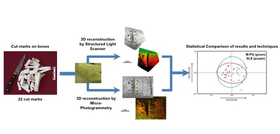
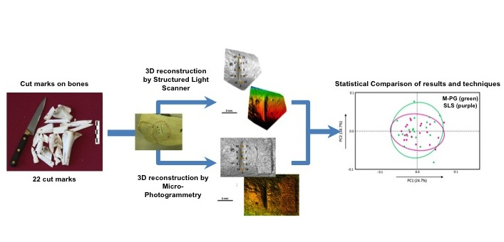
:In recent years, new techniques for the morphological study of cut marks have become essential for the interpretation of prehistoric butchering practices. Different criteria have been suggested for the description and classification of cut marks. The methods commonly used for the study of cut marks rely on high-cost microscopy techniques with low portability (i.e., inability to work in situ), such as the 3D digital microscope (3D DM) or laser scanning confocal microscopy (LSCM). Recently, new algorithmic developments in the field of computer vision and photogrammetry, have achieved very high precision and resolution, offering a portable and low-cost alternative to microscopic techniques. However, the photogrammetric techniques present some disadvantages, such as longer data collection and processing time, and the requirement of some photogrammetric expertise for the calibration of the cameras and the acquisition of precise image orientation. In this paper, we compare two low-cost techniques and their application to cut mark studies: the micro-photogrammetry (M-PG) technique presented, developed, and validated previously, and a methodology based on the use of a structured light scanner (SLS). A total of 47 experimental cut marks, produced using a stainless steel knife, were analyzed. The data registered through virtual reconstruction was analyzed by means of three-dimensional geometric morphometrics (GMM).
1. Introduction
Recently, archaeological research has substantially changed, due to the application of new technologies and multidisciplinary approaches. The application and implementation of the latest technological advances have enhanced research, scientific dissemination, and archaeological heritage management, promoting the creation of new research methodologies. Consequently, a more precise archaeological investigation is possible nowadays, including the performance of very accurate analyses with better graphic and visual designs that also promote the dissemination of the findings to a wider audience.
Geotechnologies, especially photogrammetry and laser scanning, have long played an important role in archaeological research. Photogrammetry, as a geotechnology of taking measurements and extracting information from a series of images, has long been used to record, measure, and model archaeological structures: from small scale artefacts [1,2,3,4,5] and large scale archaeological sites [6] to complex subterranean caves [7]. Even though model accuracy depends on various factors (i.e., image network, resolution, number of images, calibration), highly accurate geometric models can be achieved [8]. However, as a passive sensing technology, photogrammetry has its limitations, such as light dependence, lack of scale, and the requirement for image texture [9].
Laser scanning, also referred to as LiDAR (light detection and ranging), is a device-to-target distance measurement technology that generates dense clouds of 3D points describing the target's geometry. Laser scanning became rapidly popular in the surveying of archaeological sites, due to its direct 3D measurement, and ease of use. The data acquisition can be efficient, and can be planned regardless of the light conditions because of active sensing, which can be critical for underground or cave measurement [10].
Obviously, both photogrammetry and laser scanning have their pros and cons. Therefore, the combination of both will satisfy most scales in archaeological research [11].
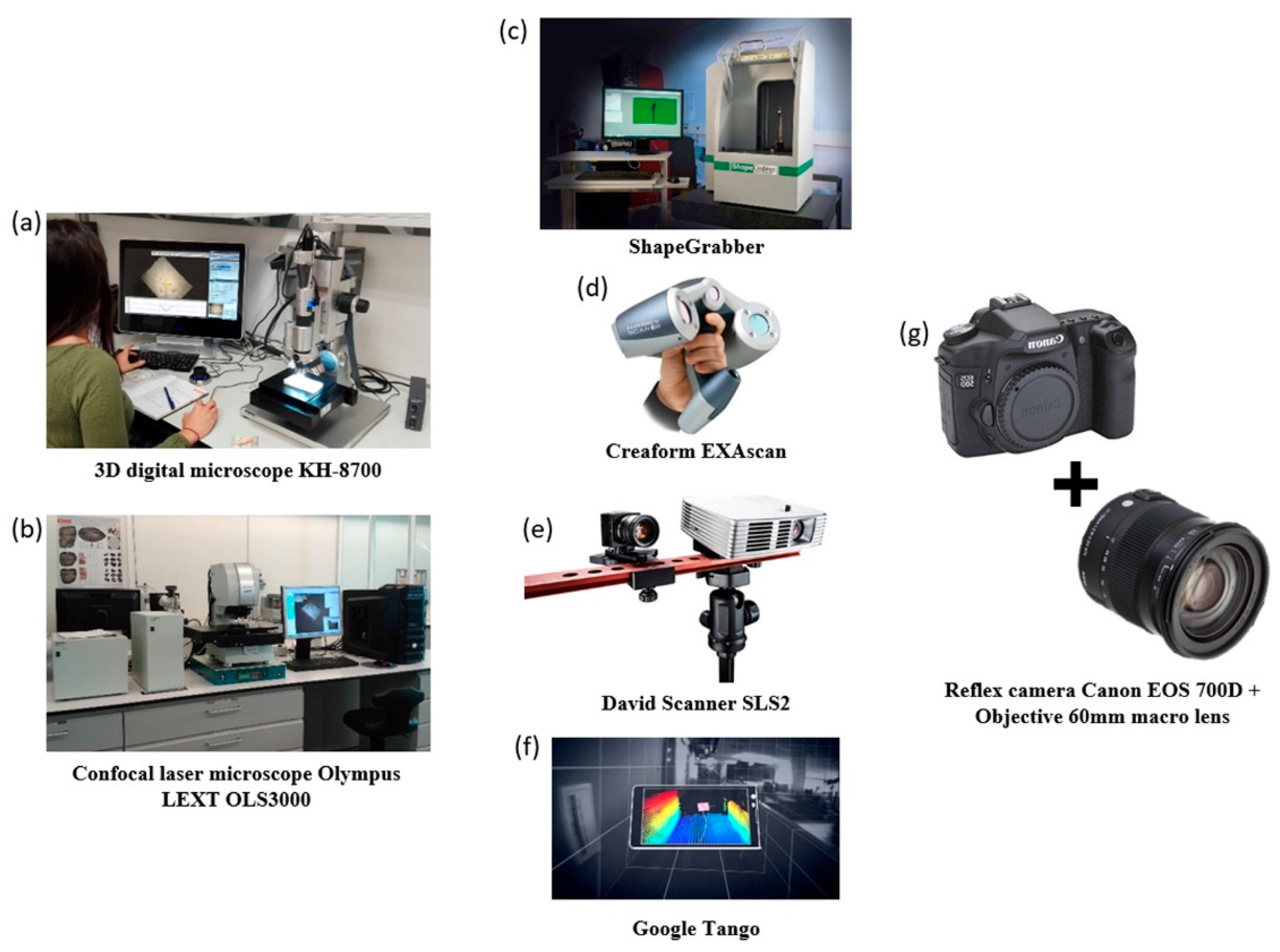
In taphonomy, microscopic techniques [12,13,14,15,16,17] (Figure 1a,b) (Table 1), have been essential to identify the type of tool or raw material used to process the carcasses found in the archaeological record. However, these techniques are expensive, and can only be used in the laboratory. Alternative solutions have been proposed by Maté-González et al. [18], developing a low-cost micro-photogrammetric method that allows metric and morphometric analyses of cut marks on bones (Figure 1g) (Table 1). The micro-photogrammetric method (M-PG) has even been validated by comparison with microscopic techniques [19]. The compatibility of photogrammetric and microscopic methods, and the possibility of producing comparable high-resolution three-dimensional models using any of these techniques, facilitates the exchange of information and data between different research teams. The main advantages of the M-PG technique, compared to the microscopic technique, is that it is simple, portable (direct work in fields or museums), and relatively cheap (the price of this type of system is around 1000 euros, because only a conventional reflex camera and a macro lens are necessary (Table 1)). Nevertheless, M-PG (passive sensor) techniques present some disadvantages, as they require longer data capture and processing time than microscopes (active sensors), and certain photogrammetric experience for the right development of some technical phases (e.g., orientation and calibration) [18]. There are, anyways, alternative techniques that combine shorter data capture time and processing and portability, like the handheld laser scanner with active sensors (Figure 1c–f) (Table 1). The applicability of these sensors is designed for the documentation of objects or close scenarios [20]. Given the wide range of active sensor handheld laser scanners that currently exist for 3D scanning, it is very important to select the most appropriate 3D documentation system for the specific sample and study. There is a price volatility that ranges from low-cost to medium-cost and high-cost systems [21]. Most of the current high-cost sensors in the market are based on the principle of laser light and triangulation-based systems (LL-TR), that achieve a 0.02 mm resolution [22] (Figure 1d) (Table 1). These devices stand out, thanks to their fast data collection, the ability to obtain immediate results, ease of use, suitability for field use, and the incorporation of metrological software. In archeology, these systems have been widely used for the documentation of rock art, ceramics, portable art, fossils, archaeological sites, etc. [23,24,25,26,27,28,29,30,31,32,33,34].
For its part, most of the current medium-cost systems in the market are based on the principle of structured light scanner (SLS) [35,36,37]. These systems consist of a projector and one or several cameras, and they achieve 0.05 mm resolution [22] (Figure 1e) (Table 1). SLS systems require a prior preparation, since calibration is required, and a post-production for the collection of data, since the union of the clouds of points is semiautomatic. The SLS system presents a special advantage provided by its composite arrangement (projector + camera), as these elements can be modified or replaced by other higher-quality devices. Besides, the results would not be affected by such changes, since the system must be calibrated before use. In archeology, the employment of these tools is increasing: e.g., ceramics, stone carvings, sculptures, jewelry, fossils, Neolithic gravestones, documentation of archaeological sites, etc. [38,39,40,41,42,43,44,45,46,47].
Low-cost systems arose for the videogame industry. The most commonly used low-cost system is the Kinect system (depth sensor, real-time Mobile 3d), which can be used alone, or can be incorporated to other systems, implying a large cost increase (e.g., Google Tango (Figure 1f) (Table 1), DPI-8, eyesmap, etc.). The resolution reached by these systems is around 8 mm at best [48]. In archeology, the use of these tools is proliferating for the close capture of sceneries as a complement to the terrestrial laser scanning [49]. It has also been used for documentation of stone carvings [50]. The stability and metric quality of low-cost systems (resolutions of 8 mm) cannot compete with high- or medium-range systems (resolutions of 0.02 mm and 0.05 mm, respectively).
In order to alleviate the disadvantages of the M-PG techniques, as well as those related to the active handheld laser scanner systems, here, we present a methodology based on a low-cost and improved structured light scanner (SLS-2) technique as an alternative to the study of cut marks on bone surfaces. We also compare, statistically, this methodology (in terms of precision and resolution) with a previously validated M-PG technique [19,51]. The comparison of these two techniques permits elucidating their simultaneous applicability in archaeological contexts. In addition, using structured light laser scanner (SLS-2) techniques, it is possible to obtain high resolution images that allow the study of taphonomic marks in detail and in real time, as SLS-2 requires short data collection and processing times. Thus, SLS-2 technique presents two fundamental features that enable the study of microscopic morphological details of larger samples. In this paper, we also test the capacity of SLS-2 systems to assess differences among cut marks on bones with different morphological characteristics.
2. Materials and Methods
2.1. Sample
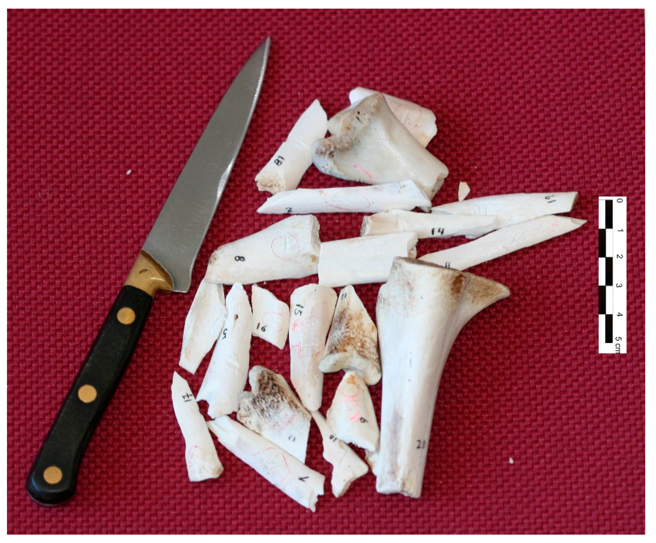
For the purpose of this study, experimental cut marks were produced using a stainless steel knife, model Molybdenum Vanadio C 0.5 CR 14 MO 0.5 VA 0.25, which allows the control of certain variables (see Maté-González et al. [19] for further details) (Figure 2). A total of 22 cut marks on an Ovis aries radius and humerus, were registered using SLS and M-PG techniques, creating 2 homologous sets of cut marks to assess differences in virtual reconstruction techniques. A second set of cut marks, reproduced using SLS, was analyzed to evaluate possible differences among cut marks on long bone epiphyses and flat bones. Radius and humerus are long bones with a more or less oval shaft, which determines cut mark section, shape, and form, when compared to cut marks performed of flat axial bones, where the curvature of bones is less, or not pronounced. In this case, a total of 21 cut marks on long bone shafts, and 26 cut marks on a scapula, were virtually reconstructed and statistically analyzed. The bones used in this second part of the study also belong to a young Ovis aries individual.
Only cut marks where the limits of the mark were clear, e.g., the start and end of the mark could be easily identified, were selected for the study. A very abnormal cut mark, according to both registration techniques (SLS and M-PG), was excluded from the analysis to avoid statistical noise.
2.2. Reflex Camera and Macro-Lens
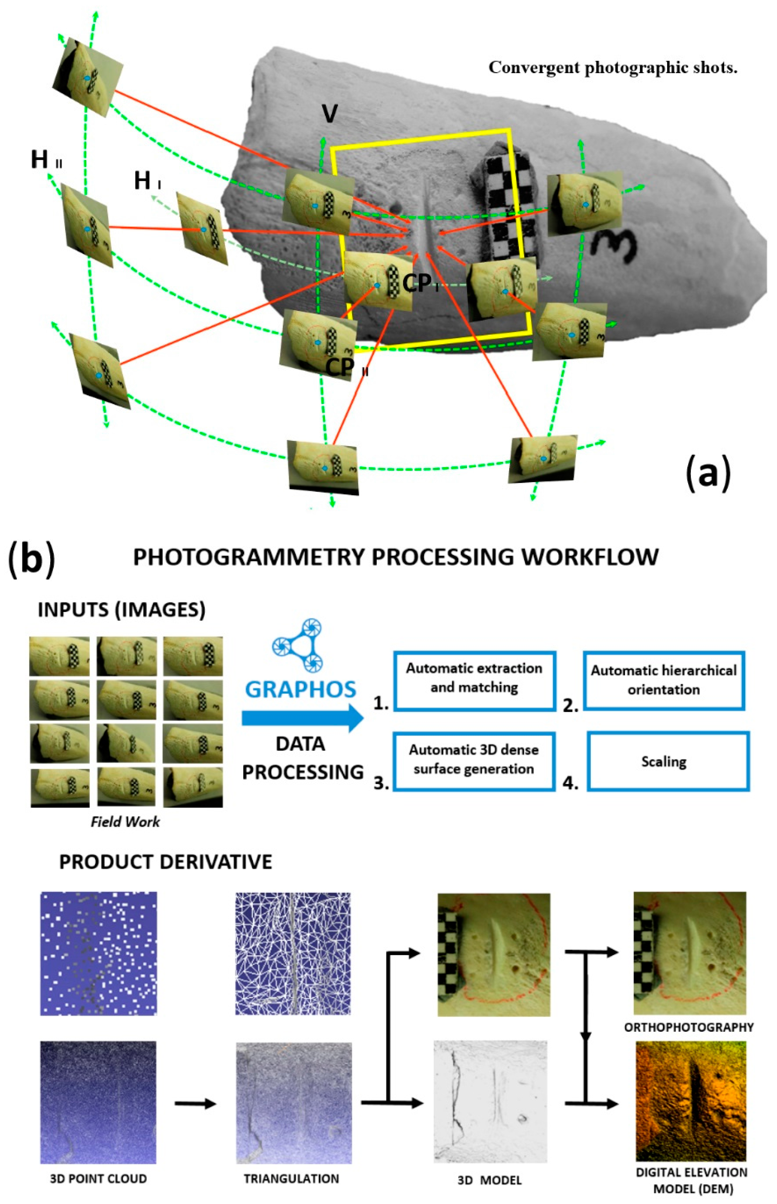
Cut marks were first registered using micro-photogrammetry (M-PG) and computer vision techniques, so as to create high-resolution 3D models of each cut mark. Precise metrical models were generated using images taken with vertical and oblique photography, using a CANON EOS 700D with a 60 mm macro lens (Table 2), and following the specified protocol explained in Maté-González et al. [18]. The camera was self-calibrated to simultaneously compute the interior and exterior camera parameters [52]. A total of 9–13 photos were taken for each mark, depending on the geometry of the bone and the shape of the mark (Figure 3a). The 3D reconstruction of a single mark took 25–30 min depending on the number of photos acquired. Photographs were processed with the open-source photogrammetric reconstruction software GRAPHOS (inteGRAted PHOtogrammetric Suite) [53,54] to generate a 3D model for each mark (Figure 3b). The scaled 3D models were exported as PLY files, and subsequently registered and studied by means of Geometric Morphometrics.
2.3. Structured Light Scanner
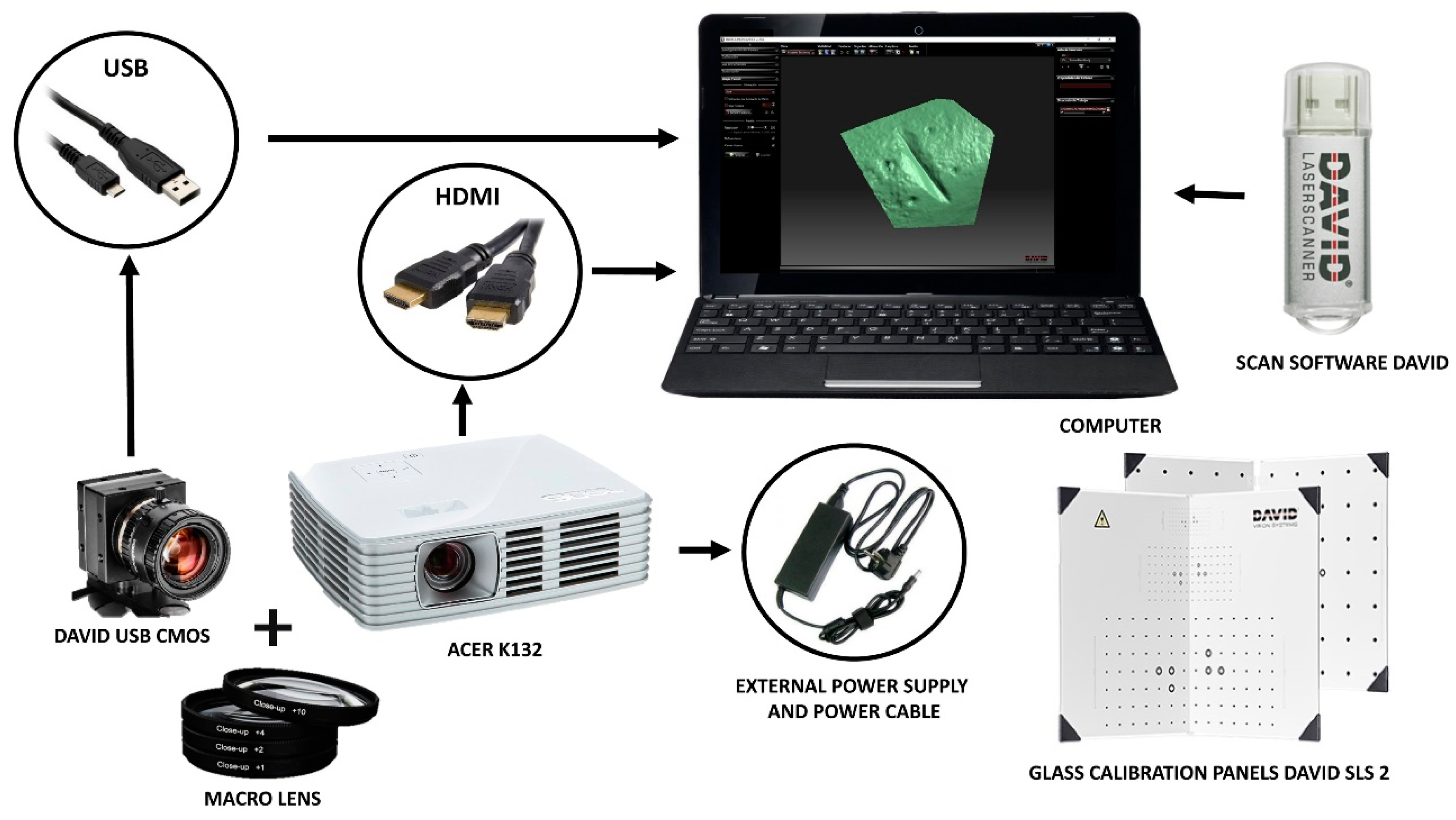
Cut marks were also digitalized with a DAVID structured-light scanner SLS-2 (Table 3), a newer version of the former DAVID SLS-1 which was improved with a macro lens getting better resolutions. This equipment, located at the C.A.I. of Archaeometry at the Complutense University of Madrid, consists in a camera, a projector, and a calibration marker board that in the first phase, needs to be calibrated (Figure 4). To carry out this process, a DAVID USB CMOS Monochrome camera is positioned and fit with a macro lens alongside an ACER K132 projector, both facing towards the calibration marker board at an angle between 15° and 25° (Figure 5a). The projection produced by the projector has to cover the entire calibration marker board, in our case, the size and calibration pattern corresponds to a 15 mm scale. Within the DAVID software, the scale is introduced as displayed on the calibration marker board, the camera’s exposure is adjusted accordingly while the focus of all the single instruments is adjusted. The equipment is then calibrated. During this process, the camera, as well as the projector, must remain fixed and stable.
The second phase consists in substituting the calibration marker board for the bone we intend to scan. The DAVID structured-light scanner SLS-2 can produce a density of up to 1.2 million points. The use of this scanning process provides a real reproduction of the bone external topography (Figure 5b). In this case, the matt polished surface of the bones avoids problems related to light intensity, or the contrast of lights and shadows during data collection. The active sensor reduces data capture time to less than 1 min. The DAVID structured-light scanner SLS-2 used in this experiment produced a higher quality resolution than the scanner used in Maté-González et al. [18].
2.4. Statistical Comparison
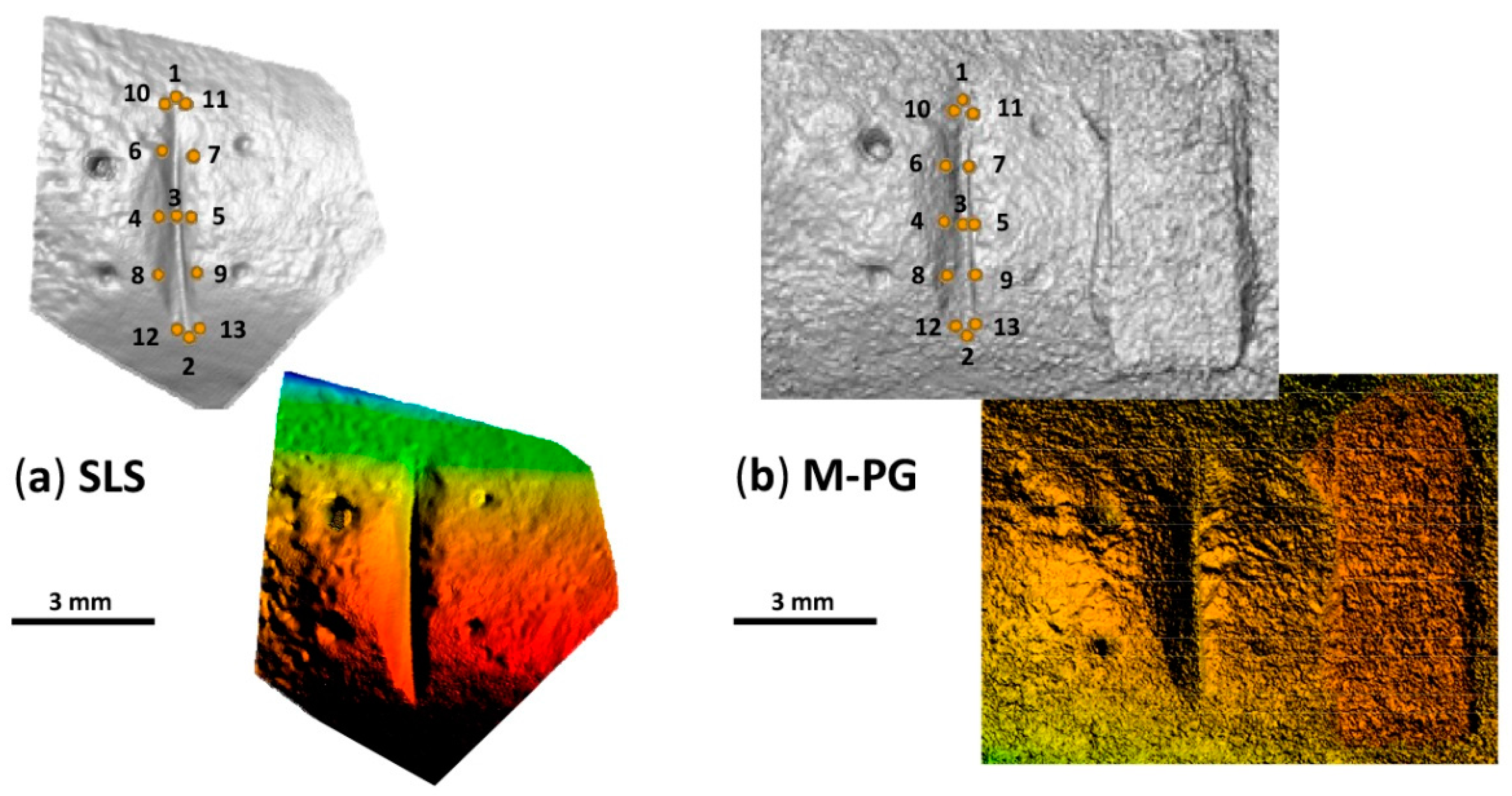
For the purpose of this study, 13 landmarks located on the exterior and interior of the mark groove were used to describe the cut marks, following the model proposed by Courtenay et al. [55] (Figure 6). This model has been proved to better capture the morphological information of cut marks when using 3D techniques, including the opening angle of the mark, and the location of its central deepest point. The landmarking step was performed in Avizo (Visualisation Sciences Group, USA).
Landmarks are homologous points that contain shape and size information in the form of Cartesian coordinates, allowing the comparison among different elements [56,57,58,59]. Landmark configurations can be analyzed by means of geometric morphometric procedures based on a Procrustes superimposition, also called generalized procrustes analysis (GPA). This technique takes the landmark data, and normalizes the form information by the application of superimposition procedures (translation, rotation and scaling). After GPA, the remaining differences between the structures, defined by landmarks, expose patterns of variation and covariation that can be studied using common multivariate statistics [60,61,62].
Several principal component analyses (PCA) performed in MorphoJ [63] and Morphologika 2.5 [56] were used to assess patterns of variation among the data in shape and form space, to study shape and size differences among cut marks. Form spaces, containing size and shape information, were obtained by re-scaling data using the natural logarithm of centroid size. Changes in shape and form space were visualized with the aid of transformation grids and warpings [64] computed using thin-plate splines.
Several tests were performed to assess differences and similarities among (1) registration techniques, and (2) cut marks on cylindrical and flat bones. The presence of defined groups was statistically tested using a multiple variance analysis (MANOVA) on the principal components (PC) scores, and analyses of variance (ANOVA) when the condition of variance homogeneity was fulfilled according to the Levene’s test. When samples showed unequal variances, the Welch’s t-test was performed to test the null hypothesis of equal means among groups. Variance analyses were performed in the free software R [65].
3. Results and Discussion
3.1. SLS vs. M-PG
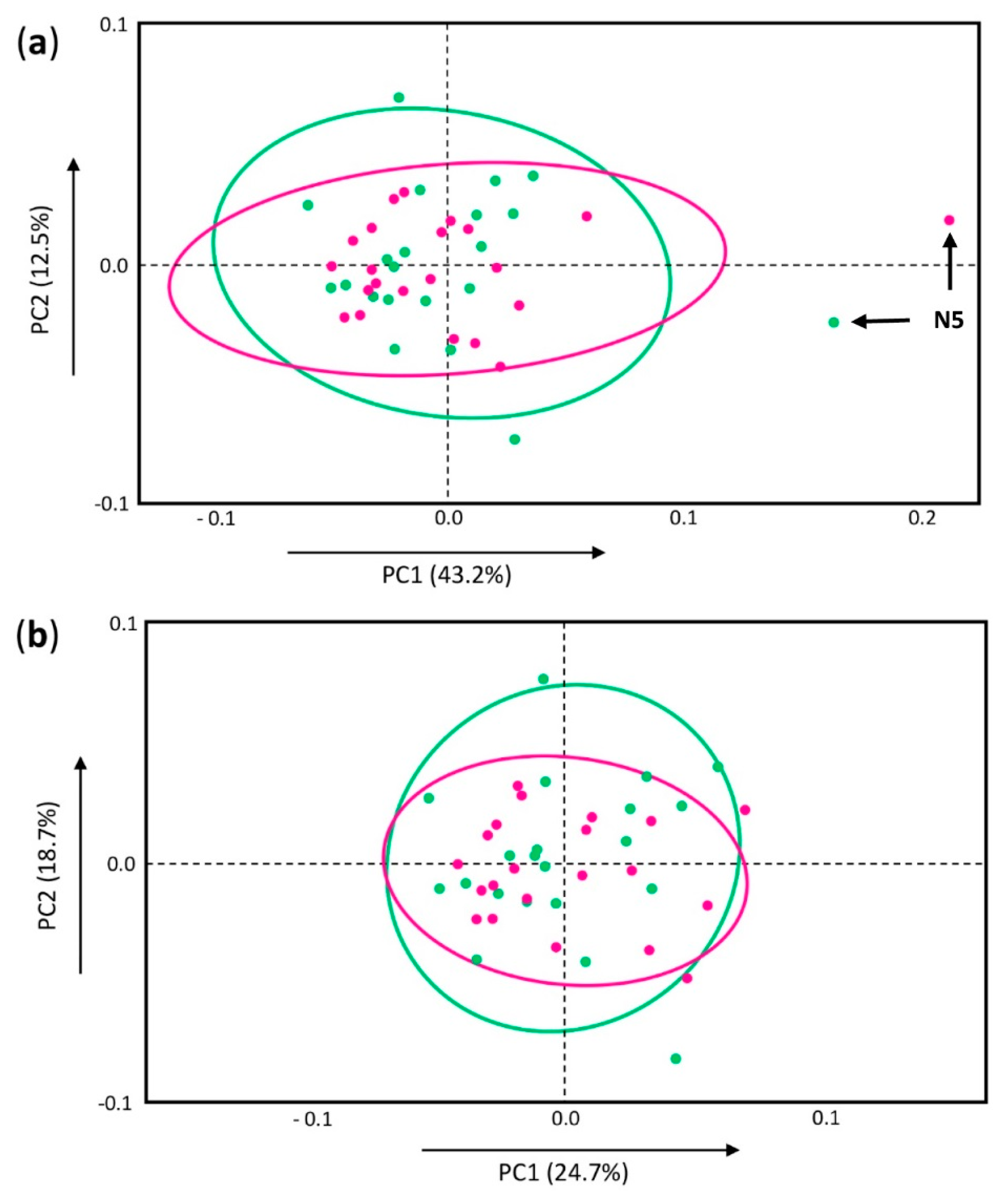
The whole sample, consisting of 22 homologous 3D models (i.e., pairs of 3D models obtained with SLS and M-PG), was subjected to a PCA, where two outliers representing the same cut mark (N 5) can be observed (Figure 7a). Since differences between this mark (N 5) and the rest of the sample are due to the nature of the cut mark itself, as it appears clearly separated when registered using both techniques, tests were run leaving the outlier out of the study, to avoid noise. However, numerical results obtained with and without the outlier are similar, and do no show significant differences between methodologies.
The cut marks registered by means of M-PG and SLS-2, overlap considerably in the second PCA plot, where less than 50% of the total variance is explained (Figure 7b). However, a slight difference can be noticed, as cut mark models generated using M-PG show a greater dispersion that expresses larger variance. Nevertheless, this larger variance among cut marks registered using M-PG methods seems to be mainly produced by only two specific marks that are clearly separated from the main scatter range.
Variance analyses (MANOVA, ANOVA) conducted on the principal component (PC) scores and assessing a greater variance percentage than the one observed in the PCA plot, support the results depicted in the graph. Both the MANOVA and ANOVA results (Table 4) highlight that there is no significant difference (p-value > 0.05) between the models generated by means of M-PG and the SLS-2. In fact, the Levene’s test performed on the sample confirmed the homogeneity of the variance in both groups (p-value > 0.05). Equally, differences between registration techniques were assessed in form space, where changes in size are also considered alongside shape, resulting in no significant differences (Table 4).
A jackknife cross-validated LDA was performed to assess minimal variance within cut mark groups, and maximal variance between groups, extracting a confusion matrix that indicates high confusion rates between the cut marks registered with M-PG techniques and the SLS-2 (Table 5). Though misclassified marks do never surpass the 50%, the Procrustes and Mahalanobis distances calculated between the groups, and the permutation tests run to assess their significance, stress that the two groups cannot be distinguished (Procrustes distance p-value = 0.44, Mahalonobis distance p-value = 0.47).
According to our statistical results, cut marks registered using M-PG and SLS-2 show no significant difference, and can thus be equally applied for the study of cut marks. In this way, the use of the SLS method would be validated in taphonomic contexts, becoming a supplementary technique that can be added to previously investigated microscopic and photogrammetric techniques.
3.2. Cut Marks on Long Bone Diaphyses vs. Cut Marks on Flat Bones
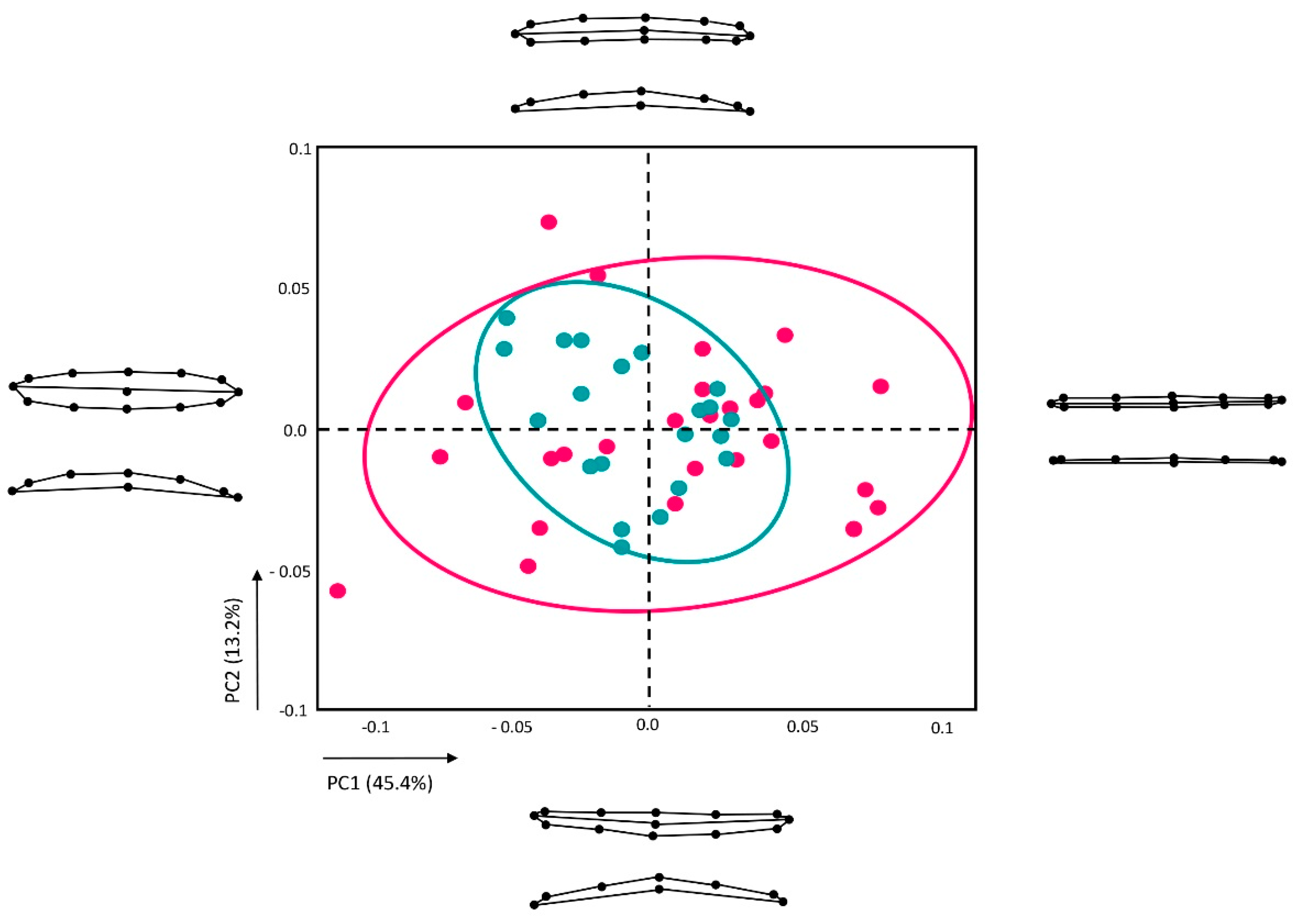
The PCA of the cut marks in shape space shows a non-polarized morphospace, defined by a high number of PCs. The scatter-plot in Figure 8 expresses only 53.1% of the total variance. In shape space, cut marks on the scapula (flat bone) appear more widely distributed than the cut marks produced on the humerus and the radius (long bones) that are mainly concentrated in the center of the graph. Though both groups clearly overlap, the shape of the cut marks on flat bones tends to be more variable, especially in relation to changes in shape expressed by PC1, that is described in its positive axis by flat and narrow cut mark shapes, and in its negative limit by wider and more curved shapes. Most cut marks registered on the scapula are closer to the narrow and flat shape, but variance in this sample is still quite large. The cut marks generated on long bone diaphyses tend to be closer to the mean shape, and mostly change along PC2, which is explained by changes in the direction of the curvature of the mark. However, in most cases, cut marks on long bones are distributed along the negative x-axis, indicating that these marks tend to be wider, deeper, and more curved. This description is consistent with the nature of long bone shafts.
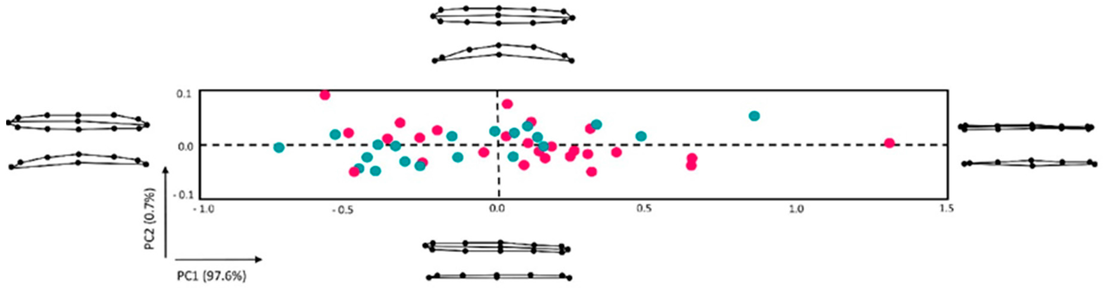
The PCA in form space is quite different, with both groups of cut marks similarly distributed along the graph, especially along PC1 (Figure 9). The first principal component is closely related to changes in centroid size that are remarkable as changes in width. Despite the scattering of the sample in the plot, two tendencies can be noticed in relation to the nature of the bones, where cut marks haven been generated: cut marks on long bones tend to gather mostly in the central or negative area of the x-axis, which corresponds to wider, deeper, and more curved forms, while 69.2% of cut marks on the scapula appear on the positive area of the x-axis, equivalent to narrower and flatter marks. Such changes in form expressed in PC1 make up 97.6% of the total variance, while PC2 only explains 0.68% of the variance and is determined by the same variables that characterize PC1 in shape space. Cut marks on long bones are similarly scattered along the positive and negative ranges of the second principal component, whereas cut marks on flat bones mostly fall in the negative range of the y-axis, determined by flatter and narrower mark forms.
The visual overlapping of cut mark groups in the PCA plots needs to be further investigated, since those graphs are two-dimensional representations of the first two PCs. Thus, the scatter-plots, first, fail to explain the entirety of the variance expressed by the sample, and, second, cannot display the distance among groups in the z-axis.
The MANOVAs performed on the PC scores to assess the differences among group means show no significant differences in shape (Wilks’ Lambda = 0.8529, F = 1.414, p = 0.2395) and form space (Wilks’ Lambda = 0.9137, F = 0.7747, p = 0.536). However, the Levene’s test indicates that variance among groups is unequal in shape and form space, and Welch’s tests were needed to confirm the similarity of the group means (Table 4). On top of that, the confusion matrix calculated shows that confusion rates between cut marks on flat and long bones are not that high and that most of the marks can be correctly classified (Table 5).
Despite graphical overlapping and statistical non-significant results in some cases, it cannot be disregarded that there is an interesting difference in the variance range of each sample, with cut marks on long bones being more concentrated in a specific area of the graph, in response to a stronger influence of bone morphology. Therefore, further experimentations are necessary to assess differences in variance distribution depending on the characteristics of the bone. The future enlargement of the experimental sample would help characterize cut marks on different bones and identify possible patterns related to bone morphology.
4. Conclusions
In this paper, we present a low-cost, portable and accurate technology for the analysis of marks on bone surfaces. The use of structured light scanners in this research area has been statistically validated by comparison with the results obtained using photogrammetric methods. Structured light scanners present remarkable advantages over photogrammetric methods, especially the time needed for data collection and processing. Particularly, the time required for the reconstruction of cut marks using SLS-2 is lower (only a few seconds) than the time required with M-PG (around 25 min). Regarding the quality of results (precision and resolution) obtained, the incorporation of a specific system of lenses to the low-cost David SLS-2 system allows us to reach a resolution of 0.016 mm and a precision equivalent to the M-PG (±0.017 mm [51]).
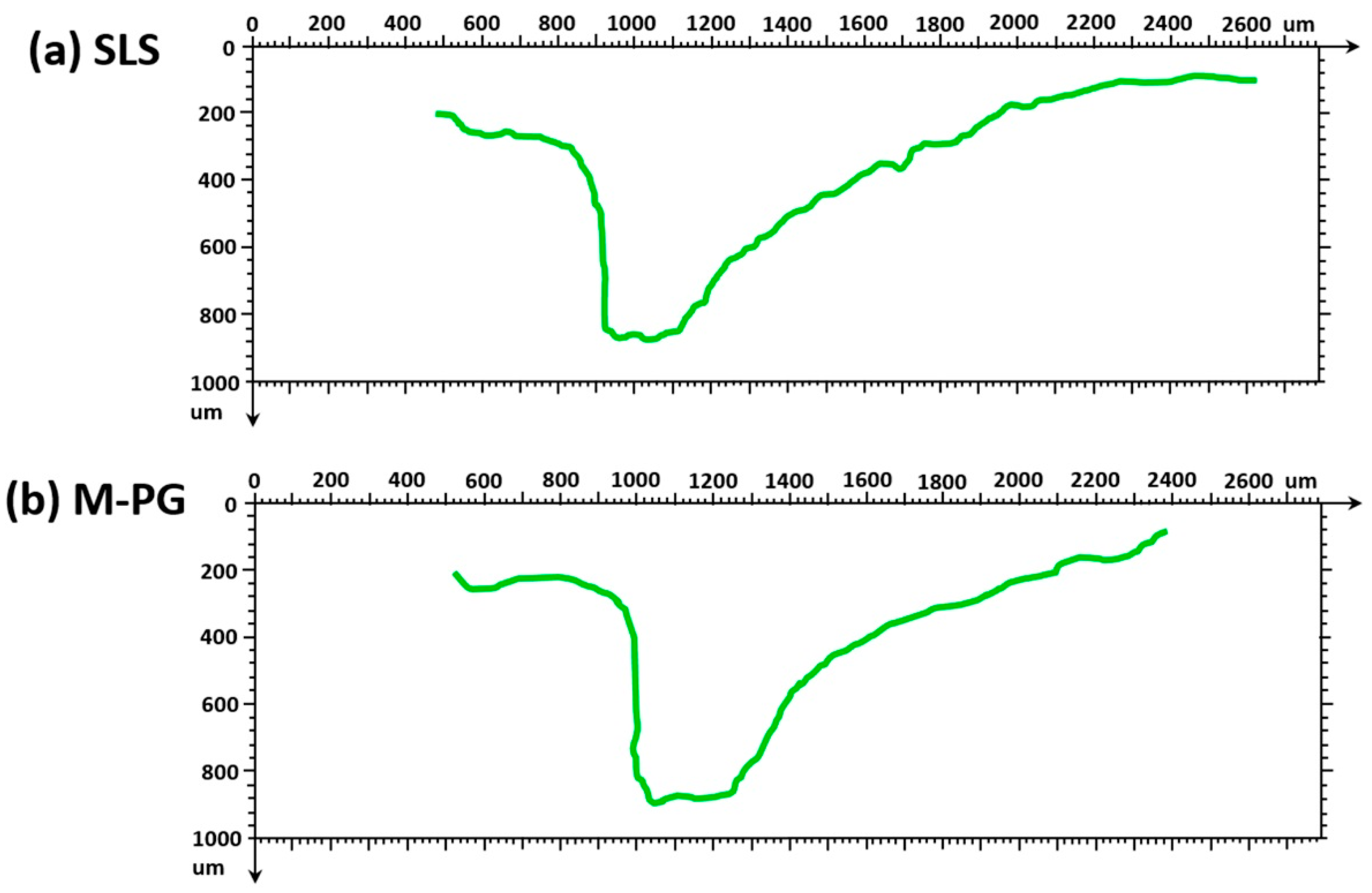
As shown in this paper, results obtained with both techniques are statistically identical, allowing the combination of SLS and M-PG for the study of certain taphonomic traces. Beyond that, structured light scanners do not only permit the application of the technique to the study of marks, but they also provide sufficient resolution to assess differences among very similar marks. Three-dimensional reconstructions generated with an improved DAVID structured light scanner have sufficient resolution so as to compare cut marks produced with the same raw material (stainless steel knife) on cylindrical (long bones) and flat bones (axial element). The resolution obtained with SLS-2 technique opens a new range of possibilities for taphonomic studies, making it possible to observe and analyze morphological differences of microscopic marks in much greater detail (Figure 10). The implementation of SLS to archaeological research would, thus, enhance statistical studies and enable the proposal of a broader range of taphonomic questions, including hypotheses on subtle morphological features.
Here, we assessed the performance of SLS-2 in morphological studies on bone surface modifications. However, the method could be extended to other types of surfaces to study the shape and size features of different elements, such as engravings on portable or parietal art.
Although the results obtained in this study are very satisfactory and demonstrate the validity of this low-cost method for the study of conspicuous and well-defined marks (e.g., cut marks), the SLS-2 technique still shows the same difficulties when carrying out studies of more loosely defined marks (e.g., trampling marks), as it was the case with M-PG techniques. It is true that the SLS-2 technique achieves a better resolution than M-PG (Figure 10), but still lacks sufficient resolution to register the subtleties of fine microscopic details.
Researchers now have a low-cost method at their disposal that overcomes the limitations encountered when using microscopes (e.g., restricted access due to high costs), providing fast and accurate results. Accordingly, analytical costs and time might reduce, facilitating an increase in processed sample sizes.
Acknowledgments
We would like to thank the TIDOP Group from the Department of Cartographic and Land Engineering of the High Polytechnics School of Avila, University of Salamanca, for the use of tools and facilities. We want to recognize the technical support provided by C.A.I. Arqueometry and Archaeological Analysis from Complutense University which has been very useful to carry out the present work. Julia Aramendi would like to thank the Spanish Education, Culture and Sports Ministry (FPU15/04585) for funding her postgraduate education program.
Author Contributions
Miguel Ángel Maté-González—Cut marks 3D registration using SLS techniques; Julia Aramendi—Statistical analyses; Diego González-Aguilera—Cut marks 3D registration using M-PG techniquesJosé Yravedra—Experimental works; All the authors contributed to the drafting of this paper.
Conflicts of Interest
The authors declare no conflicts of interest.
References
- Kersten, T.P.; Lindstaedt, M. Image-Based Low-Cost Systems for Automatic 3D Recording and Modelling of Archaeological Finds and Objects. In ICP in Cultural Heritage Preservation; Springer: Berlin/Heidelberg, Germany, 2012; pp. 1–10. [Google Scholar]
- Tiano, P.; Tapete, D.; Matteini, M.; Ceccaroni, F. The microphotogrammetry: A new diagnostic tool for on site monitoring of monumental surfaces. In Proceedings of the International Workshop SMW08, Florence, Italy, 27–29 October 2008; pp. 97–106. [Google Scholar]
- Aramendi, J.; Maté-González, M.A.; Yravedra, J.; Ortega, M.C.; Arriaza, M.C.; González-Aguilera, D.; Baquedano, E.; Domínguez-Rodrigo, M. Discerning carnivore agency through the three-dimensional study of tooth pits: Revisiting crocodile feeding behaviour at FLK-Zinj and FLK NN3 (Olduvai Gorge, Tanzania). Palaeogeogr. Palaeoclimatol. Palaeoecol. 2017. [Google Scholar] [CrossRef]
- Gajski, D.; Solter, A.; Gašparović, M. Applications of macro photogrammetry in archaeology. In Proceedings of the XXIII ISPRS Congress, Prague, Czech Republic, 12–19 July 2016. [Google Scholar]
- Cachero, R.; Abello, C. Stereo-photometric techniques for scanning micrometer scale. Virtual Archaeol. Rev. 2015, 6, 72–76. [Google Scholar] [CrossRef]
- Reu, J.D.; Plets, G.; Verhoeven, G.; Smedt, P.D.; Bats, M.; Cherretté, B.; Maeyer, W.D.; Deconynck, J.; Herremans, D.; Laloo, P. Towards a three-dimensional cost-effective registration of the archaeological heritage. J. Archaeol. Sci. 2013, 40, 1108–1121. [Google Scholar] [CrossRef]
- Chandler, J.H.; Fryer, J.G. Recording aboriginal rock art using cheap digital cameras and digital photogrammetry. In Proceedings of the CIPA XX International Symposium, Torino, Italy, 26 September–1 October 2005. [Google Scholar]
- Koutsoudis, A.; Vidmar, B.; Ioannakis, G.; Arnaoutoglou, F.; Pavlidis, G.; Chamzas, C. Multi-image 3D reconstruction data evaluation. J. Cult. Herit. 2014, 15, 73–79. [Google Scholar] [CrossRef]
- Dhonju, H.; Xiao, W.; Sarhosis, V.; Mills, J.P.; Wilkinson, S.; Wang, Z.; Thapa, L.; Panday, U.S. Feasibility Study of Low-Cost Image-Based Heritage Documentation in Nepal. In International Archives of the Photogrammetry; Remote Sensing and Spatial Information Sciences: Göttingen, Germany, 2017; pp. 237–242. [Google Scholar]
- González-Aguilera, D.; Muñoz-Nieto, Á.; Rodríguez-Gonzálvez, P.; Menéndez, M. New tools for rock art modelling: Automated sensor integration in Pindal Cave. J. Archaeol. Sci. 2011, 38, 120–128. [Google Scholar] [CrossRef]
- El-Hakim, S.F.; Beraldin, J.A.; Picard, M.; Godin, G. Detailed 3D reconstruction of large-scale heritage sites with integrated techniques. IEEE Comput. Graph. Appl. 2004, 24, 21–29. [Google Scholar] [CrossRef] [PubMed]
- Bello, S.M.; Soligo, C. A new method for the quantitative analysis of cutmark micromorphology. J. Archaeol. Sci. 2008, 35, 1542–1552. [Google Scholar] [CrossRef]
- Bello, S.M. New Results from the Examination of Cut-Marks Using Three-Dimensional Imaging. In The Ancient Human Occupation of Britain; Ashton, N., Lewis, S.G., Stringer, C., Eds.; Elsevier: Amsterdam, The Netherlands, 2011; pp. 249–262. ISBN 9780444535986. [Google Scholar]
- Boschin, F.; Crezzini, J. Morphometrical Analysis on Cut Marks Using a 3D Digital Microscope. Int. J. Osteoarch. 2012, 22, 549–562. [Google Scholar] [CrossRef]
- Archer, W.; Braun, D.R. Investigating the signature of aquatic resource use within Pleistocene hominin dietary adaptations. PLoS ONE 2013, 8, e69899. [Google Scholar] [CrossRef] [PubMed] [Green Version]
- Crezzini, J.; Boschin, F.; Wierer, U. Wild cats and cut marks: Exploitation of Felis silvestris in the Mesolithic of Galgenbühel/Dos de la Forca (South Tyrol, Italy). Q. Int. 2014, 330, 52–60. [Google Scholar] [CrossRef]
- Bonney, H. An investigation of the use of discriminant analysis for the classification of blade edge type from cut marks made by metal and bamboo blades. Am. J. Phys. Anthropol. 2014, 154, 575–584. [Google Scholar] [CrossRef] [PubMed]
- Maté-González, M.Á.; Yravedra, J.; González-Aguilera, D.; Palomeque-González, J.F.; Domínguez-Rodrigo, M. Micro-photogrammetric characterization of cut marks on bones. J. Archaeol. Sci. 2015, 62, 128–142. [Google Scholar] [CrossRef]
- Maté-González, M.Á.; Aramendi, J.; Yravedra, J.; Blasco, R.; Rosell, J.; González-Aguilera, D.; Domínguez-Rodrigo, M. Assessment of Statistical Agreement of Three Techniques for the Study of Cut Marks: 3D Digital Microscope, Laser Scanning Confocal Microscopy and Micro-Photogrammetry. J. Micro Technol. 2017. [Google Scholar] [CrossRef] [PubMed]
- Calvache, A.T.M.; García, J.L.P.; Colmenero, V.B.; Arenas, A.L. Estudio geométrico de piezas arqueológicas a partir de un modelo virtual 3D. Virtual Archaeol. Rev. 2011, 2, 109–113. [Google Scholar] [CrossRef]
- Kersten, T.P.; Przybilla, H.J.; Lindstaedt, M.; Tschirschwitz, F.; Misgaiski-Hass, M. Comparative Geometrical Investigations of Hand-Held Scanning Systems. Int. Soc. Photogram. Remote Sens. 2016. [Google Scholar] [CrossRef]
- Remondino, F. Heritage recording and 3D modeling with photogrammetry and 3D scanning. Remote Sens. 2011, 3, 1104–1138. [Google Scholar] [CrossRef] [Green Version]
- Allard, T.; Sitchon, M.; Sawatzky, R.; Hoppa, R. Use of hand-held laser scanning and 3D printing for creation of a museum exhibit. In Proceedings of the 6th International Symposium on Virtual Reality, Archaelogy and Cultural Heritage, Pisa, Italy, 8–11 November 2005. [Google Scholar]
- Park, H.K.; Chung, J.W.; Kho, H.S. Use of hand-held laser scanning in the assessment of craniometry. Forensic Sci. Int. 2006, 160, 200–206. [Google Scholar] [CrossRef] [PubMed]
- Munkelt, C.; Bräuer-Burchardt, C.; Kühmstedt, P.; Schmidt, I.; Notni, G. Cordless hand-held optical 3D sensor. Proc. SPIE 2007. [Google Scholar] [CrossRef]
- Cano, P.; Lamolda, F.; Torres, J.C.; del Mar Villafranca, M. Uso de escáner láser 3D para el registro del estado previo a la intervención de la Fuente de los Leones de La Alhambra. Virtual Archaeol. Rev. 2010, 1, 89–94. [Google Scholar] [CrossRef]
- Melero, F.J.; León, A.; Torres, J.C. Digitalización y reconstrucción de elementos cerámicos arqueológicos de torno. Virtual Archaeol. Rev. 2010, 1, 137–141. [Google Scholar] [CrossRef]
- Escarcena, J.C.; de Castro, E.M.; García, J.L.P.; Calvache, A.M.; del Castillo, T.F.; García, J.D.; Cámara, M.U.; Castillo, J.C. Integration of photogrammetric and terrestrial laser scanning techniques for heritage documentation. Virtual Archaeol. Rev. 2011, 2, 53–57. [Google Scholar] [CrossRef]
- Kühmstedt, P.; Bräuer-Burchardt, C.; Schmidt, I.; Heinze, M.; Breitbarth, A.; Notni, G. Hand-held 3D Sensor for Documentation of Fossil and Archaeological Excavations. 2011. Avaliable online: http://olymp.inf-cv.uni-jena.de:6680/pdf/Kuhmstedt11:HHT.pdf (accessed on 22 August 2017).
- Boyd, C.P.; Marín, F.M.; Goodmaster, C.; Johnson, A.; Castaneda, A.; Dwyer, B. Digital Documentation and the Archaeology of the Lower Pecos Canyonlands. Virtual Archaeol. Rev. 2012, 3, 98–103. [Google Scholar] [CrossRef]
- Komar, D.A.; Davy-Jow, S.; Decker, S.J. The Use of a 3-D Laser Scanner to Document Ephemeral Evidence at Crime Scenes and Postmortem Examinations. J. Forensic Sci. 2012, 57, 188–191. [Google Scholar] [CrossRef] [PubMed]
- Neamtu, C.; Popescu, S.; Popescu, D.; Mateescu, R. Using reverse engineering in archaeology: Ceramic pottery reconstruction. J. Autom. Mobile Robot. Intell. Syst. 2012, 6, 55–59. [Google Scholar]
- Comes, R.; Buna, Z.; Badiu, I. Creation and preservation of digital cultural heritage. J. Am. Heart Assoc. 2014, 1, 10–15. [Google Scholar]
- Manferdini, A.M.; Gasperoni, S.; Guidi, F.; Marchesi, M. Unveiling Damnatio Memoriae. The use of 3D digital technologies for the virtual reconstruction of archaeological finds and artefacts. Virtual Archaeol. Rev. 2016, 7, 9–17. [Google Scholar] [CrossRef]
- Rodríguez-Martín, M.; Rodríguez-Gonzálvez, P.; González-Aguilera, D.; Fernández-Hernández, J. Feasibility Study of a Structured Light System Applied to Welding Inspection Based on Articulated Coordinate Measure Machine Data. IEEE Sens. J. 2017, 17, 4217–4224. [Google Scholar] [CrossRef]
- Santoso, F.; Garratt, M.A.; Pickering, M.R.; Asikuzzaman, M. 3D Mapping for Visualization of Rigid Structures: A Review and Comparative Study. IEEE Sens. J. 2016, 16, 1484–1507. [Google Scholar] [CrossRef]
- Blais, F.; Rioux, M.; Beraldin, J.A. Practical considerations for a design of a high precision 3D laser scanner system. Proc. SPIE 1988, 959, 225–246. [Google Scholar]
- Stumpfel, J.; Tchou, C.; Yun, N.; Martinez, P.; Hawkins, T.; Jones, A.; Debevec, P.E. Digital Reunification of the Parthenon and its Sculptures. In Proceedings of the 4th International conference on Virtual Reality, Archaeology and Intelligent Cultural Heritage, Brighton, UK, 5–7 November 2003; Volume 1, pp. 41–50. [Google Scholar]
- Akca, D.; Remondino, F.; NovÃ, D.; Hanusch, T.; Schrotter, G. Recording and modeling of cultural heritage objects with coded structured light projection systems. In Proceedings of the 2nd International Conference on Remote Sensing in Archaeology, Rome, Italy, 4–7 December 2006; pp. 375–382. [Google Scholar]
- McPherron, S.P.; Gernat, T.; Hublin, J.J. Structured light scanning for high-resolution documentation of in situ archaeological finds. J. Archaeol. Sci. 2009, 36, 19–24. [Google Scholar] [CrossRef]
- Niven, L.; Steele, T.E.; Finke, H.; Gernat, T.; Hublin, J.J. Virtual skeletons: Using a structured light scanner to create a 3D faunal comparative collection. J. Archaeol. Sci. 2009, 36, 2018–2023. [Google Scholar] [CrossRef]
- Georgopoulos, A.; Ioannidis, C.; Valanis, A. Assessing the performance of a structured light scanner. ISPRS Int. Arch. Photogram. Remote Sen. Spat. Inf. Sci. 2010, 38, 250–255. [Google Scholar]
- Slizewski, A.; Friess, M.; Semal, P. Surface scanning of anthropological specimens: Nominal-actual comparison with low cost laser scanner and high end fringe light projection surface scanning systems. Quartär 2010, 57, 179–187. [Google Scholar]
- Ahmed, N.; Carter, M.; Ferris, N. Sustainable archaeology through progressive assembly 3D digitization. World Archaeol. 2014, 46, 137–154. [Google Scholar] [CrossRef]
- Neiß, M.; Sholts, S.B.; Wärmländer, S.K. New applications of 3D modeling in artefact analysis: Three case studies of Viking Age brooches. Archaeol. Anthropol. Sci. 2016, 8, 651–662. [Google Scholar] [CrossRef]
- Errickson, D.; Grueso, I.; Griffith, S.J.; Setchell, J.M.; Thompson, T.J.U.; Thompson, C.E.L.; Gowland, R.L. Towards a Best Practice for the Use of Active Non-contact Surface Scanning to Record Human Skeletal Remains from Archaeological Contexts. Inter. J. Osteoarchaeol. 2017. [Google Scholar] [CrossRef]
- Kuzminsky, S.C.; Tung, T.A.; Hubbe, M.; Villaseñor-Marchal, A. The application of 3D geometric morphometrics and laser surface scanning to investigate the standardization of cranial vault modification in the Andes. J. Archaeol. Sci. Rep. 2017, 10, 507–513. [Google Scholar] [CrossRef]
- Gonzalez-Jorge, H.; Rodríguez-Gonzálvez, P.; Martínez-Sánchez, J.; González-Aguilera, D.; Arias, P.; Gesto, M.; Díaz-Vilariño, L. Metrological comparison between Kinect I and Kinect II sensors. Measurement 2015, 70, 21–26. [Google Scholar] [CrossRef]
- Kersten, T.P.; Omelanowsky, D.; Lindstaedt, M. Investigations of Low-Cost Systems for 3D Reconstruction of Small Objects. In Euro-Mediterranean Conference; Springer International Publishing: Cham, Switzerland, 2016; pp. 521–532. [Google Scholar]
- Pomaska, G. Monitoring the deterioration of stone at Mindener Museum’s Lapidarium. ISPRS Int. Arch. Photogram. Remote Sens. Spatial Inf. Sci. 2013, XL-5/W2, 495–500. [Google Scholar] [CrossRef]
- Yravedra, J.; Maté-González, M.Á.; Palomeque-González, J.F.; Aramendi, J.; Estaca-Gómez, V.; San Juan Blazquez, M.; García Vargas, E.; Organista, E.; González-Aguilera, D.; Arriaza, M.C.; et al. A new approach to raw material use in the exploitation of animal carcasses at BK (Upper Bed II, Olduvai Gorge, Tanzania): A micro-photogrammetric and geometric morphometric analysis of cut marks. Boreas 2017. [Google Scholar] [CrossRef]
- Fraser, C. Multiple focal setting self-calibration of close-range metric cameras. Photogram. Eng. Remote Sens. 1980, 46, 1161–1171. [Google Scholar]
- González-Aguilera, D.; López-Fernández, L.; Rodríguez-González, P.; Guerrero-Sevilla, D.; Hernández-López, D.; Menna, F.; Nocerino, E.; Toschi, I.; Remondino, F.; Ballabeni, A.; et al. Development of an All-Purpose Free Photogrammetric Tool; ISPRS International Archives: Prague, Czech Republic, 2016. [Google Scholar]
- González-Aguilera, D.; López-Fernández, L.; Rodríguez-González, P.; Guerrero-Sevilla, D.; Hernández-López, D.; Menna, F.; Nocerino, E.; Toschi, I.; Remondino, F.; Ballabeni, A.; et al. InteGRAted Photogrammetric Suite, GRAPHOS. In Proceedings of the Congress: CATCON7-ISPRS, Prague, Czech Republic, 12–19 July 2016. [Google Scholar]
- Courtenay, L.; Yravedra, J.; Mate-González, M.Á.; Aramendi, J.; González-Aguilera, D. 3D Analysis of Cut Marks Using a New Geometric Morphometric Methodological Approach. Archaeol. Anthropol. Sci. 2017. Accepted. [Google Scholar]
- O’Higgins, P.; Johnson, D. The Quantitative Description and Comparison of Biological Forms. Critic. Rev. Anatom. Sci. 1988, 1, 149–170. [Google Scholar]
- Bookstein, F. Types of Landmarks, Morphometric Tools for Landmark Data: Geometry and Biology; Cambridge University Press: New York, NY, USA, 1991; pp. 63–64. [Google Scholar]
- Hall, B. Descent with Modification: The unity underlying homology and homoplasy as seen through an analysis of development and evolution. Biol. Rev. 2003, 78, 409–433. [Google Scholar] [CrossRef] [PubMed]
- Klingenberg, C. Novelty and “Homology-Free” Morphometrics: What’s in a Name? Evol. Biol. 2008, 35, 186–190. [Google Scholar] [CrossRef]
- Richtsmeier, J.T.; Deleon, V.B.; Lele, S.R. The promise of geometric morphometrics. Am. J. Phys. Anthropol. 2002, 45, 63–91. [Google Scholar] [CrossRef]
- Rohlf, F.J. Shape Statistics: Procrustes Superimpositions and Tangent Spaces. J. Classif. 1999, 16, 197–223. [Google Scholar] [CrossRef]
- Slice, D.E. Landmark Coordinates Aligned by Procrustes Analysis Do Not Lie in Kendall’s Shape Space. Syst. Biol. 2001, 50, 141–149. [Google Scholar] [CrossRef] [PubMed]
- Klingenberg, H. MorphoJ: An integrated software package for geometric morphometrics. Mol. Ecol. Resour. 2011, 11, 353–357. [Google Scholar] [CrossRef] [PubMed]
- Bookstein, F. Principal Warps: Thin-Plate Spline and the Decomposition of Deformations. Trans. Pattern A Mach. Intell. 1989, 11, 567–585. [Google Scholar] [CrossRef]
- Core-Team. R: A Language and Environment for Statistical Computing; R Foundation for Statistical Computing: Vienna, Austria, 2015; Available online: https://www.Rproject.org/ (accessed on 25 May 2017).
- Timm, N.H. Applied Multivariate Analysis; Springer: New York, NY, USA, 2002. [Google Scholar]
Figure 1.
(a) 3D digital microscope KH-8700, (b) Confocal laser microscope Olympus LEXT OLS3000, (c) Triangulation-based ShapeGrabber, (d) Creafrom EXAscan, (e) Structured Light David Scanner SLS2 (f) Google Tango, (g) Reflex Canon EOS 700D + Objective 60 mm macro lens.
Figure 1.
(a) 3D digital microscope KH-8700, (b) Confocal laser microscope Olympus LEXT OLS3000, (c) Triangulation-based ShapeGrabber, (d) Creafrom EXAscan, (e) Structured Light David Scanner SLS2 (f) Google Tango, (g) Reflex Canon EOS 700D + Objective 60 mm macro lens.

Figure 2.
Stainless steel knife used in the study to create the cut marks on several bones.

Figure 3.
(a) Protocol for image capture to model a cut mark on a bone by the micro-photogrammetry method, with convergent photographic shots. CP, Master and dependent images in central position. V, Vertical slave images. H, Horizontal slave images. (b) Workflow of the image-based modelling technique.

Figure 4.
DAVID structured-light scanner SLS-2 technical equipment. It should be noted, the macro lens used to improve the SLS-2 resolution.
Figure 4.
DAVID structured-light scanner SLS-2 technical equipment. It should be noted, the macro lens used to improve the SLS-2 resolution.

Figure 5.
(a) Arrangement of the structured-light scanner equipment to perform a 3D scanning. (b) 3D scanning and results obtained from data collection.
Figure 5.
(a) Arrangement of the structured-light scanner equipment to perform a 3D scanning. (b) 3D scanning and results obtained from data collection.
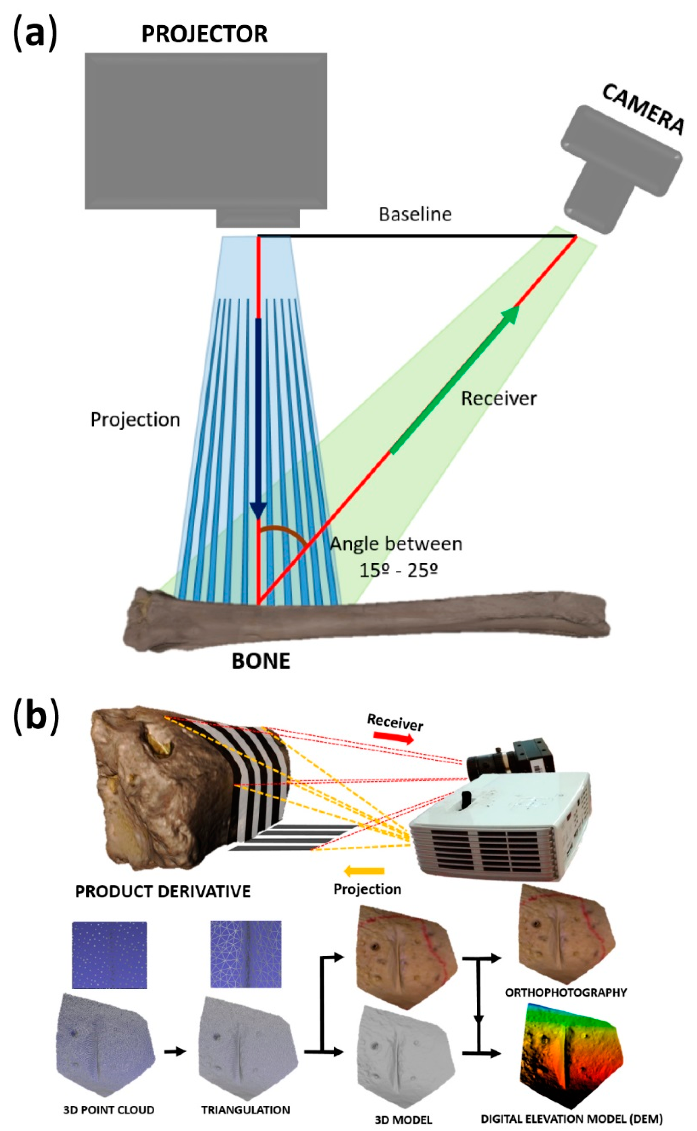
Figure 6.
Landmarks used to describe cut marks registered using (a) SLS and (b) M-PG techniques as suggested in Courtenay (2017).
Figure 6.
Landmarks used to describe cut marks registered using (a) SLS and (b) M-PG techniques as suggested in Courtenay (2017).

Figure 7.
Principal component analyses (PCA) in shape space of the homologous cut mark reconstructions performed with M-PG (green) and with DAVID SLS-2 (purple). (a) Graph including the whole sample. (b) Second PCA performed removing the outlier (N5).
Figure 7.
Principal component analyses (PCA) in shape space of the homologous cut mark reconstructions performed with M-PG (green) and with DAVID SLS-2 (purple). (a) Graph including the whole sample. (b) Second PCA performed removing the outlier (N5).

Figure 8.
PCA plot where shape variance among cut marks on long bones (green) and flat bones (pink) is expressed. Shape changes are visualized for PC1 and PC2 positive and negative axis ends.
Figure 8.
PCA plot where shape variance among cut marks on long bones (green) and flat bones (pink) is expressed. Shape changes are visualized for PC1 and PC2 positive and negative axis ends.

Figure 9.
PCA plot where form variance among cut marks on long bones (green) and flat bones (pink) is expressed. Form changes are visualized for PC1 and PC2 positive and negative axis ends.
Figure 9.
PCA plot where form variance among cut marks on long bones (green) and flat bones (pink) is expressed. Form changes are visualized for PC1 and PC2 positive and negative axis ends.

Figure 10.
Profiles extracted from 3D reconstructions of the same cut mark performed using (a) SLS-2, and (b) M-PG techniques.
Figure 10.
Profiles extracted from 3D reconstructions of the same cut mark performed using (a) SLS-2, and (b) M-PG techniques.


Table 1.
Comparison between different measuring techniques.
| Technical | Measuring Procedure | Classification | System | Portability | Speed (min) | Range | Usage Way | Resolution | Cost [EUR] |
|---|---|---|---|---|---|---|---|---|---|
| Microscopy | 3D digital microscope | Active sensor | KH-8700 | low | >1 | 1–10 mm | Automatic | 0.15–0.01 μm | <100.000 |
| confocal laser microscope | Active sensor | Olympus LEXT OLS3000 | low | >1 | 1–20 mm | Automatic | 0.12–0.01 μm | <100.000 | |
| Laser scanners | Triangulation-based | Active sensor | ShapeGrabber | medium | >1 | 21–120 cm | Automatic | 0.02 mm | <30.000 |
| Structured Light | Active sensor | Creaform EXAscan | high | >1 | 0.17–0.40 m | Automatic | 0.05 mm | <20.000 | |
| Structured Light | Active sensor | David Scanner SLS2 | medium | >1 | 0.15–5.00 m | Semiautomatic | 0.02 mm | 3.000 | |
| Time-of-flight | Active sensor | Google Tango | high | >1 | 0.50–4.00 m | Automatic | 8 mm | 450 | |
| Photogrammetry | Micro-photogrammetry | Passive sensor | Reflex + macro objective | high | ≅25 | 10–50 cm | Semiautomatic | 0.02 mm | 1000 |
Table 2.
Technical specifications of the photographic sensor with macro lens (Canon EOS 700D).
| Canon EOS 700D | |
|---|---|
| Type | CMOS |
| Sensor size | 22.3 × 14.9 mm |
| Pixel size | 4.3 μm |
| Image size | 5184 × 3456 pixels |
| Total pixels | 18.0 MP |
| Focal length | 60 mm |
| Focused distance to object | 100–120 mm |
Table 3.
Technical specifications of the Structured Light Scanner SLS-2.
| DAVID Structured-Light Scanner SLS-2 | |
|---|---|
| Workpiece size | 16 × 500 mm |
| Resolution | Up to 0.1% of scan size (down to 0.016 mm) |
| Scanning time | One single scan within a few seconds |
| Mesh density | Up to 12,000,000 vertices per scan |
Table 4.
Mean comparison between cut mark samples. CM = Cut mark; LB = Long bone; FB = Flat bone.
| Sample | F | p-Value | |
|---|---|---|---|
| MANOVA in shape space | SLS-2 vs. M-PG | 0.4904 | 0.7812 |
| MANOVA in form space | SLS-2 vs. M-PG | 1.33 | 0.2739 |
| ANOVA in shape space | SLS-2 vs. M-PG | 0.5242 | 0.718 |
| Welch t-test in form space | SLS-2 vs. M-PG | 3.345 | 0.998 |
| MANOVA in shape space | CM on LB vs. CM on FB | 1.414 | 0.2395 |
| MANOVA in form space | CM on LB vs. CM on FB | 0.7747 | 0.536 |
| Welch t-test in shape space | CM on LB vs. CM on FB | 0.9202 | 0.4552 |
| Welch t-test in form space | CM on LB vs. CM on FB | 1.076 | 0.989 |
Table 5.
Cross-validated confusion matrices calculated for the different cut mark groups analyzed. CM a = Cut mark; LB b = Long bone; FB c = Flat bone.
Table 5.
Cross-validated confusion matrices calculated for the different cut mark groups analyzed. CM a = Cut mark; LB b = Long bone; FB c = Flat bone.
| CM a on LB b with SLS-2 | CM a on LB b with M-PG | CM a on LB b | CM a on FB c | Total | |
|---|---|---|---|---|---|
| CM a on LB b with SLS-2 | 13 (61.9%) | 8 (38.1%) | 21 | ||
| CM a on LB b with M-PG | 8 (38.1%) | 13 (61.9%) | 21 | ||
| CM a on LB b | 14 (66.7%) | 7 (33.3%) | 21 | ||
| CM a on FBc | 7 (26.9%) | 19 (73.1%) | 26 |
© 2017 by the authors. Licensee MDPI, Basel, Switzerland. This article is an open access article distributed under the terms and conditions of the Creative Commons Attribution (CC BY) license (http://creativecommons.org/licenses/by/4.0/).
Share and Cite
MDPI and ACS Style
Maté-González, M.Á.; Aramendi, J.; González-Aguilera, D.; Yravedra, J. Statistical Comparison between Low-Cost Methods for 3D Characterization of Cut-Marks on Bones. Remote Sens. 2017, 9, 873. https://doi.org/10.3390/rs9090873
AMA Style
Maté-González MÁ, Aramendi J, González-Aguilera D, Yravedra J. Statistical Comparison between Low-Cost Methods for 3D Characterization of Cut-Marks on Bones. Remote Sensing. 2017; 9(9):873. https://doi.org/10.3390/rs9090873
Chicago/Turabian StyleMaté-González, Miguel Ángel, Julia Aramendi, Diego González-Aguilera, and José Yravedra. 2017. "Statistical Comparison between Low-Cost Methods for 3D Characterization of Cut-Marks on Bones" Remote Sensing 9, no. 9: 873. https://doi.org/10.3390/rs9090873
Note that from the first issue of 2016, this journal uses article numbers instead of page numbers. See further details here.