On-Board Ortho-Rectification for Images Based on an FPGA
by
Guoqing Zhou Rongting Zhang Na Liu Jingjin Huang and Xiang Zhou
1,2,3, 
Rongting Zhang
1,2,3,*,
Na Liu
1,
Jingjin Huang
2,3 and
Xiang Zhou
1,3 1
Guangxi Key Laboratory for Spatial Information and Geomatics, Guilin University of Technology, Guilin 541004, China
2
College of Precision Instrument and Opto-Electronic Engineering, Tianjin University, Tianjin 300072, China
3
The Center for Remote Sensing, Tianjin University, Tianjin 300072, China
*
Author to whom correspondence should be addressed.
Remote Sens. 2017, 9(9), 874; https://doi.org/10.3390/rs9090874
Submission received: 16 June 2017
/
Revised: 7 August 2017
/
Accepted: 18 August 2017
/
Published: 23 August 2017
Abstract
:The traditional ortho-rectification technique for remotely sensed (RS) images, which is performed on the basis of a ground image processing platform, has been unable to meet timeliness or near timeliness requirements. To solve this problem, this paper presents research on an ortho-rectification technique based on a field programmable gate array (FPGA) platform that can be implemented on board spacecraft for (near) real-time processing. The proposed FPGA-based ortho-rectification method contains three modules, i.e., a memory module, a coordinate transformation module (including the transformation from geodetic coordinates to photo coordinates, and the transformation from photo coordinates to scanning coordinates), and an interpolation module. Two datasets, aerial images located in central Denver, Colorado, USA, and an aerial image from the example dataset of ERDAS IMAGINE 9.2, are used to validate the processing speed and accuracy. Compared to traditional ortho-rectification technology, the throughput from the proposed FPGA-based platform and the personal computer (PC)-based platform are 11,182.3 kilopixels per second and 2582.9 kilopixels per second, respectively. This means that the proposed FPGA-based platform is 4.3 times faster than the PC-based platform for processing the same RS images. In addition, the root-mean-square errors of the planimetric coordinates φX and φY and the distance φS are 1.09 m, 1.61 m, and 1.93 m, respectively, which can meet the requirements of correction accuracy in practice.
1. Introduction
Given technological development, remotely sensed (RS) images can be acquired quickly and easily. However, the speed of image processing cannot catch up with the speed of obtaining remote sensing images because of the limitations of image processing technology. Conventionally, to process the acquired images (such as mosaic, fusion, and ortho-rectification), they need to be sent back to the ground performance center. Moreover, many traditional image processing systems, such as ENVI and ERDAS IMAGINE, are serial instruction systems based on personal computer (PC) computers. Thus, these image processing systems hardly meet the demand in response of time-critical disasters, making the abundant image resources underutilized.
Ortho-rectification is an essential step in RS image processing, which aims to remove the geometric distortions and obtain the mapping-based geographic coordinates of the image. It is important for and the basis of the subsequent image processing and applications. The traditional ortho-rectification methods correct images and remove distortion pixel-by-pixel using a personal computer (PC)-based platform on the basis of a digital elevation model (DEM). It is difficult to achieve a demand for (near) real-time performance because the processing unit is a pixel and there is a great amount of image data. On the other hand, since the algorithm complexity of ortho-rectification is very high, serial instruction processing systems take much time to perform the ortho-rectification algorithms. Thus, how to improve the speed of the ortho-rectification process has become an urgent issue when applied in on-board processing of a spacecraft.
Due to the limitation of the speed of serial instruction processing, many parallel processing methods for image processing have been proposed, such as [1,2,3,4,5,6]. Pan et al. [1] presented a fast motion estimation method to reduce the encoding complexity of the H.265/HEVC encoder implemented by Intel Xeon CPU E5-1620 v2 (Intel company, 2200 Mission College Blvd, Santa Clara, CA 95054-1549, USA). and random access memory (RAM). Jiang et al. [2] proposed a scalable massively parallel fast research algorithm to reduce the computational cost of motion estimation and disparity estimation using a central processing unit (CPU)/ graphical processing unit (GPU). In these methods, the GPU and CPU are combined to process images. Although the ground parallel processing system had improved the speed of image processing, the RS images needed to be sent back to the ground processing centers. Within the entire process, much time is still wasted. Additionally, most of the parallel processing methods are based on the multiple task operating system of the GPU, which cannot essentially solve the problem of a serial instruction method.
An effective solution for the (near) real-time processing of image ortho-rectification is to perform the ortho-rectification on hardware. In recent decades, the field programmable gate array (FPGA) has been widely used in the image processing (such as imaging compression [7,8], filtering [9,10,11], edge detection [12,13], real-time processing of video images [14,15], and motion estimation [16,17,18]) to make real-time processing come true. González et al. [16,17] optimized matching-based motion estimation algorithms using an Altera custom instruction-based paradigm and a combination of synchronous dynamic random access memory (SDRAM) and on-chip memory in Nios II processors, and presented a low-cost system. Botella et al. [18] proposed an architecture for a neuromorphic robust optical flow based on FPGA, which was applied in a difficult environment. In addition to a very-high-speed integrated circuit hardware description language (VHDL) and Verilog HDL, OpenCL is usually used to design an FPGA [19,20]. Waidyasooriya et al. [19] proposed an FPGA architecture for three-dimensional (3-D) finite difference time domain (FDTD) acceleration applying OpenCL, which solved the problem of designing time. Rodriguez-Donate et al. [20] evaluated the use of a convolution operator in signal processing disciplines focused on FPGA evaluation under different optimizations with respect to thread and memory level exploitation, in which OpenCL was used. In the RS community, although there is also some research on applying FPGA to the real-time processing of RS images, it is still not enough to meet the requirement in practice. For example, Thomas et al. [21] and Kalomiros et al. [22] proposed an image processing system by combining software and hardware that can improve the speed of image correction and mosaicing. David et al. [23] presented a processing method whereby the computing process is migrated to an FPGA, which aimed at solving the problem when the number of pixels in an image was huge and the transformation calculation of the floating-point matrix was complex. Through applying the characteristics of FPGA parallel computing, the proposed method by David and Don [23] improved the speed of image correction. Winfried et al. [24] designed an on-board bispectral infrared detection (BIRD) system based on the neural network processor NI1000, a digital signal processor (DSP), and an FPGA. The system can perform on-board radiometric correction, geometric correction, and texture extraction. Malik et al. [25] built a quick process hardware platform using an FPGA. The hardware platform could process 390 frames of 640 × 480 images per second. Tomasi et al. [26] researched a stereo vision algorithm based on an FPGA to perform the correction of video graphics array (VGA) images (57 fps). Pierre et al. [27] applied the pipeline method of an FPGA to correct the color of stereo video images. Kumar et al. [28] realized the real-time correction of images using an FPGA under a dynamic environment.
To our understanding, a hardware system for image correction is mainly about the field of real-time correction of video images, stereo-pair real-time correction, etc. There are few studies on ortho-rectification of RS images. Thus, this paper develops a hardware platform based on an FPGA for RS image ortho-rectification. Through decomposing the ortho-rectification algorithm, several basic algorithms of image processing can be obtained, reducing the complexity of the algorithm and reaching the purpose of (near) real-time ortho-rectification. The proposed FPGA-based ortho-rectification platform integrates three modules: a memory module, a coordinate transformation module (including the transformation from geodetic coordinates to photo coordinates and the transformation from photo coordinates to scanning coordinates), and an interpolation module.
This paper is organized as follows: the structure of the proposed hardware platform based on an FPGA is described in Section 2, and the experiments, comparison, and analyses are conducted in Section 3 and Section 4 to evaluate and validate the accuracy and real-time performance of the proposed method. Some conclusions are drawn up in Section 5.
2. FPGA Implementation for the Ortho-Rectification Algorithm
2.1. A Brief Review of the Ortho-Rectification Algorithm
Many ortho-rectification models have been proposed over the past few decades. According to the type of image, terrain of the covered area, and geomorphic features, an appropriate model can be chosen to ortho-rectify the RS images. Generally, ortho-rectification models contain a rigorous correction model based on the collinearity condition equation, a rational function model, or an affine-transformation-based correction model. In this paper, the collinearity condition equation is used to implement RS image ortho-rectification on the proposed platform. The collinearity condition equation model is based on the corresponding relationship of space geometry between the point of image space and the point of object space. The collinearity condition equation is the model that is applied to simulate and solve the position and posture of a sensor at the time of imaging. The collinearity condition equation is very suitable for various resolutions of images and the situation where the parameters of orbit are known or unknown. In this section, the collinearity condition equation model is briefly introduced.
The ortho-rectification method can be classified as the direct method and indirect method. The direct method applies the image coordinates of the original image to compute the coordinates of the ortho-photo, and the indirect method applies the image coordinates of the ortho-photo to compute the image coordinates of the original image. In this paper, the indirect method is used. The processes of the indirect method based on the collinearity condition equation include the following:
(1) The determination of the geodetic coordinates of the pixels in the ortho-photo
Let (Xg0, Yg0) be the geodetic coordinates of a marginal point on the left bottom of the ortho-photo; (I, J) be the column and row coordinates of an arbitrary pixel in the ortho-photo; Δx and Δy be the sample intervals of columns and rows, respectively; M be the scale denominator of the ortho-photo; and (Xg, Yg) be the geodetic coordinates of pixel G. The geodetic coordinates of pixel G can be obtained by
After determining the geodetic coordinates of pixels in the ortho-photo, the elevation (i.e., Zg) of each pixel can be acquired through interpolating the digital surface model (DSM).
(2) The transformation from geodetic coordinates to photo coordinates
At the time of imaging, the ground point, the center of projection, and the photo point are on a line. According to the collinearity relationship among them, the photo coordinates of the ground point can be obtained by:
where (u, v) are the photo coordinates of the ground point; x0, y0, and f are the interior orientation elements; Xs, Ys, and Zs are the exterior orientation elements; and ah, bh, and ch (h = 1, 2, 3) are the elements of the rotation matrix R that can be obtained by Equation (3).
where φ, ω, and κ are three rotational angles along the x-, y- and z-axis in coordinate transformation, respectively.
(3) The transformation from photo coordinates to scanning coordinates
Because there is affine deformation between the photo coordinate system and the scanning coordinate system, the following affine transformation is used to get the scanning coordinates for the pixels:
where mt, nt, and k′t (t = 1, 2) are the coefficients of affine transformation; (i′0, j′0) are the scanning coordinates of the principle point; specially, k1 = k′1 + i′0 and k2 = k′2 + j′0; and (i′, j′) are the scanning coordinates of an arbitrary pixel.
(4) Gray-scale bilinear interpolation
The gray-scale of pixels in the ortho-photo can be determined according to the acquired scanning coordinates. Because the obtained scanning coordinates may not only be in the center of a pixel, a gray-scale interpolation process is required. In this paper, the bilinear interpolation method is applied.
where i and j are nonnegative integers; p and q are in the range of (0, 1); and f(i, j) are gray values.
2.2. FPGA-Based Implementation for Ortho-Rectification Algorithms
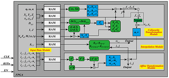
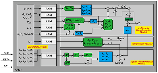
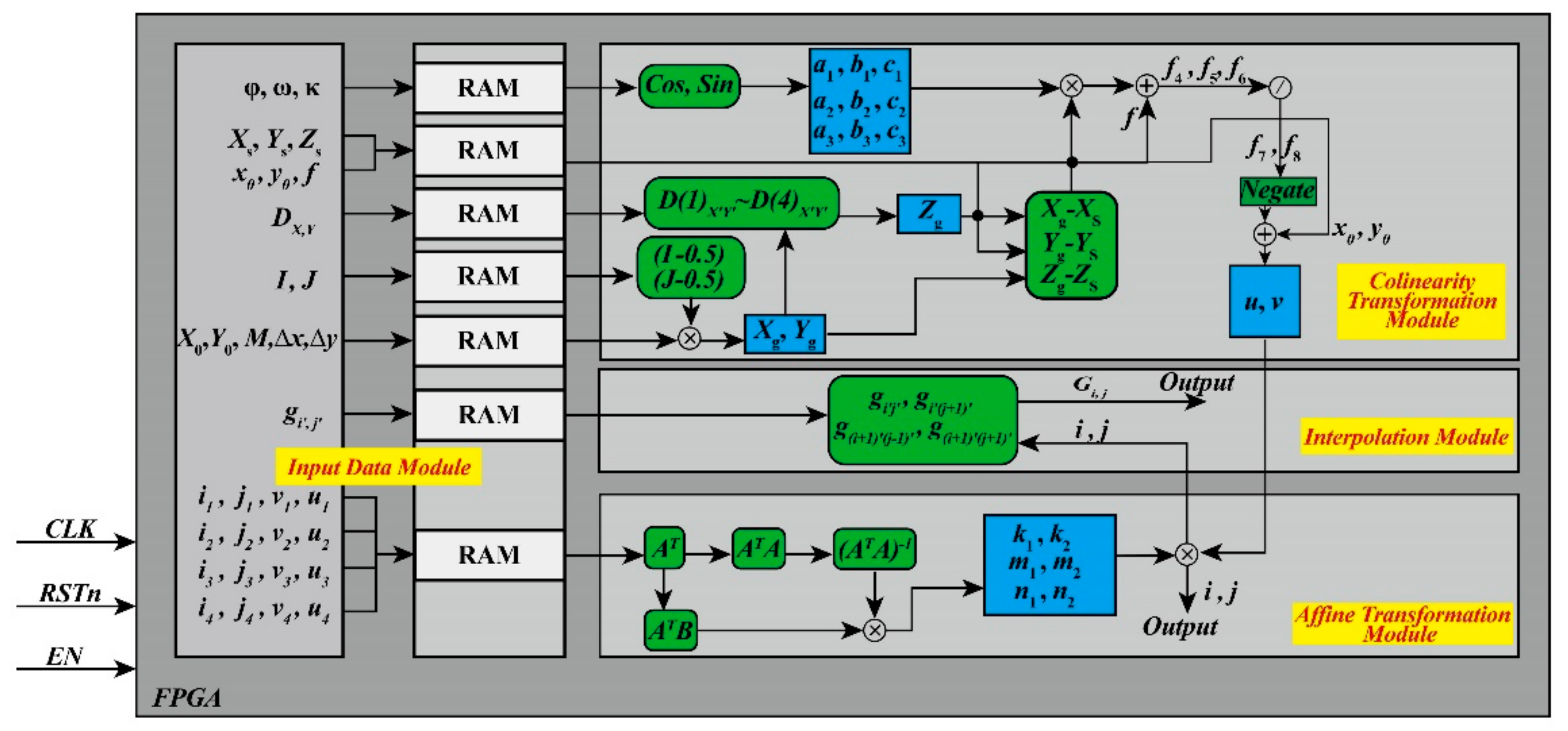
The parallel processing of an FPGA is a main research direction in the high-performance rapid calculation community. The calculation speed of an FPGA is affected by multi-factors (such as the amount of logical resource in the chosen FPGA and the optimal design of algorithms). Through analyzing the structure of an ortho-rectification algorithm and optimizing it, an FPGA-based hardware architecture for ortho-rectification was designed (as shown in Figure 1). The FPGA-based hardware architecture contains three modules: (i) an input data module; (ii) a coordinate transformation module that includes a collinearity equation transformation module (CETM) and an affine transformation module (ATM); and (iii) an interpolation module (IM). The details of these modules are described as follows.
- (1)
- The original data and parameters are stored in the RAM of the input data module. These original data and parameters are sent to the CETM, ATM, and IM in the same clock cycle, when the enable signal is being received;
- (2)
- The coefficients of the collinearity conditional equation, geodetic coordinates of the ortho-photo, and photo coordinates are calculated by the CETM. In the same clock cycle, the acquired photo coordinates are sent to the ATM;
- (3)
- The coefficients of affine transformation are calculated in the ATM and then the coefficients and photo coordinates are combined to calculate the scanning coordinates, which are sent to the IM and output in the same clock cycle;
- (4)
- The gray-scale of the ortho-photo is obtained by scanning the coordinates and cached gray-scale of the original image in the IM. In the same clock cycle, the obtained gray-scale of the ortho-photo is output to the external memory.
2.2.1. FPGA-Based Implementation for a Two-Row Buffer
As is well known, to perform bilinear interpolation, several neighborhoods of a pixel are needed. However, an FPGA is not like software for storing the whole image in the internal storage and reading the value of the image pixel according to the index. Thus, according to the size of the neighborhood, several rows of image data should be cached in advance. Moreover, the cache should be built to store the required image data. Many research studies have made efforts to design the structure of a buffer, such as [29,30,31,32]. Especially, the structure of a state machine [32] is a useful method for solving the issue of buffers.
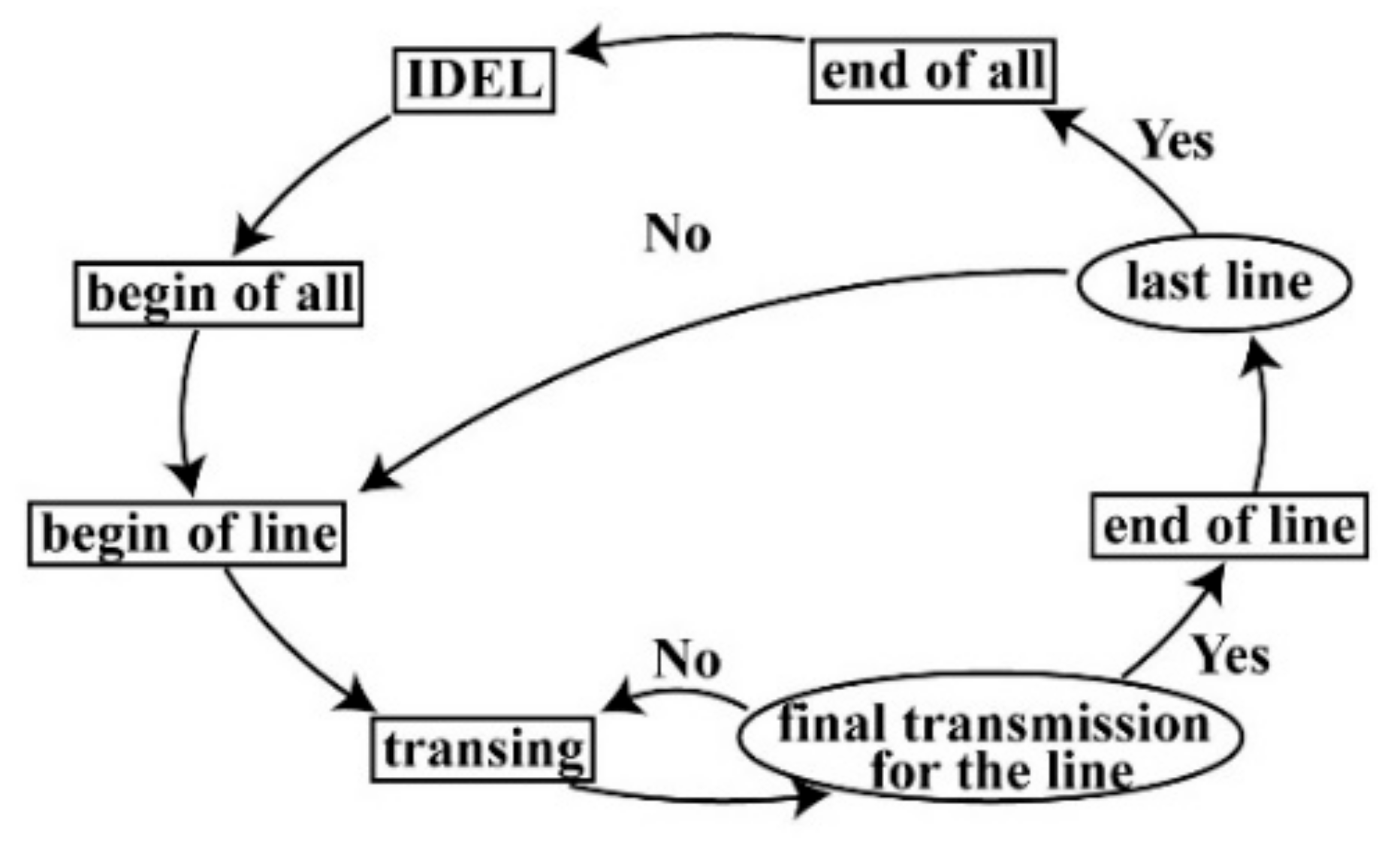
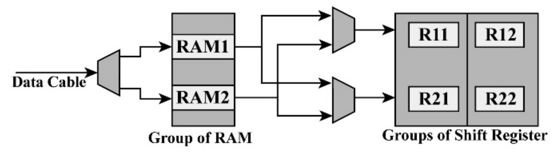
According to [32], a two-row buffer based on an FPGA is proposed. As shown in Figure 2, four states, i.e., IDEL (initialization), the beginning of all, the end of all, and beginning of the line, are used for initialization and cache cleaning. In the “transing” state, according to the control signal and the address of the reading and writing, the corresponding operations are chosen, including storing the image date in the dual RAM from the external storage, waiting for image data to be taken from the dual RAM, and turning to the “end of line” state. The number of dual RAM modules, i.e., nRAM, can be determined by the number of rows of neighbors, i.e., nnb, where nRAM is equal to nnb. To implement bilinear interpolation, 2 × 2 neighbors are needed. Thus, as shown in Figure 3, two dual RAMs are used as the cache media for the first level cache of image input. When two dual RAMs are used to buffer data, a multiplexer is exploited to determine which dual RAM should store the data. For 2 × 2 neighbors, two groups of cycle shift registers are used to store the data from neighboring pixels of the input image in the second level cache. For each group consisting of end-to-end registers, two registers, noted as Rmn (m, n = 1, 2), are contained. The data sent from the dual RAMs first are input selectors that ensure the row order is the same as the row order of the input image, and then the output of the selectors is sent to the groups of the cycle shift register. When storing the data from the dual RAMs into Rm1 each time, the data stored in Rmn (m = 1, 2, n = 1) is assigned to Rm(n+1) (m = 1, 2, n = 1), while the data stored in Rm4 (m = 1, 2) are thrown out.
2.2.2. FPGA-Based Implementation for Coordinate Transformation
According to Section 2.1, the ortho-rectification method based on the collinearity condition equation needs two coordinate transformations. As shown from Equations (1)–(4), these equations involve compound operations. However, the hardware implementation for an algorithm is based on the most basic logic operations. Thus, the ortho-rectification method based on the collinearity equation must be divided into several simple add and multiplication operations, corresponding to the hardware components of the adder and multiplier, respectively. The details of the FPGA-based implementation for coordinate transformation modules are described as follows.
(1) FPGA-based implementation for calculating geodetic coordinates Xg, Yg, and Zg
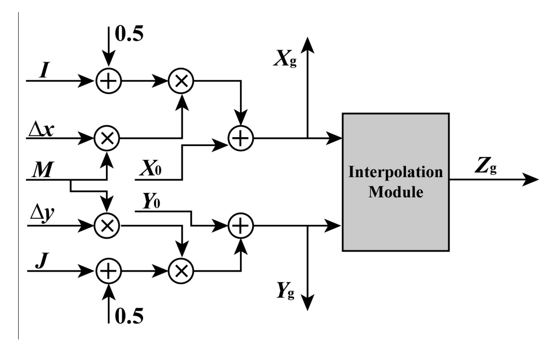
To obtain the geodetic coordinates Xg, Yg, and Zg at part (1) of Section 2.1 using an FPGA chip, a parallel computation architecture is presented in Figure 4. As shown in Figure 4, four adders and four multipliers are used to compute Xg and Yg in parallel by I, X0, Δx, M, J, Δy, and Y0, respectively. After obtaining Xg and Yg, they are sent to the interpolation module for calculating Zg. To ensure that Xg, Yg, and Zg are output in the same clock cycle, the delay units are utilized for computing processing. The details of the interpolation module are presented in the following Section 2.2.3, because its computing process is the same as gray interpolation.
(2) FPGA-based implementation for the transformation from geodetic coordinates to photo coordinates
For an FPGA-based implementation in parallel computing for the transformation from geodetic coordinates to photo coordinates, a modification of Equation (2) is needed. The intermediate variables produced in the computing process can be divided into three levels. The goal of the first level is to implement the margin calculation of the geodetic coordinates between any point and the principal point of the photograph. The first level contains:
The second level (see Equation (7)) is to calculate the products between the transformation coefficients and intermediate variables f1, f2, and f3.
The computation of the third level (see Equation (8)) is based on the first and the second levels to obtain the photo coordinates,
To compute f4, f5, and f6 in Equation (7), the elements of the rotation matrix R (i.e., ai, bi, and ci, i = 1, 2, 3) should be first calculated based on Equation (3). To compute the rotation matrix R using an FPGA chip, a parallel computation module is presented in Figure 5a, in which ai, bi, and ci (i = 1, 2, 3) are calculated by the sin and cos functions of the three rotational angles φ, ω, and κ. Through using the CORDIC IP core, the sin and cos functions can be implemented by an FPGA. To ensure that ai, bi, and ci (i = 1, 2, 3) are obtained in the same clock cycle, the delay units should be exploited in the computing process, where there are twelve multipliers and four adders.
To implement the transformation from geodetic to photo coordinates, i.e., Equations (6)–(8) using an FPGA chip, a parallel computation module is presented in Figure 5b. As shown in Figure 5b, the initial data (i.e., x0, y0, f, XS, YS, and ZS) stored in the input data module, the rotation matrix calculated by using the sin and cos functions and rotation angles, and the geodetic coordinates (Xg, Yg, and Zg) calculated by Figure 4 are used to compute the photo coordinates (u, v). In the computing process, eleven multipliers, eight adders, and two dividers are employed. Moreover, the delay units are also utilized to ensure that the outputs (u, v) are sent into the next module in the same clock cycle.
(3) FPGA-based implementation for the transformation from photo to scanning coordinates
To realize the transformation from photo to scanning coordinates using an FPGA chip, Equation (4) is divided into two levels. The first level is:
Additionally, the second level includes:
where A1 = (m1, n1) and A2 = (m2, n2) are the affine transformation coefficients, and B = (u, v)T are the photo coordinates. The transformation coefficients, i.e., ms, ns, and ks (s = 1, 2), should be calculated first based on the following least squares method.
To compute the coefficients of affine transformation, four control points are needed. Let H be the matrix of the control point scanning coordinates, Q be the matrix of the photo coordinates of the known fiducial points, and C be the matrix of the affine transformation coefficients,
According to the least squares method, Equation (15) can be solved by:
• FPGA-based implementation for QTQ and QTH
To implement the matrix multiplication QTQ based on an FPGA chip, it can be rewritten using an optimum method. As shown in Equation (17), the elements of the matrix contain three formats, i.e., “a1 + b1 + c1 + d1”, “a12 + b12 + c12 + d12”, and “a1a2 + b1 b2 + c1c2 + d1d2”. Moreover, the matrix of G = QTQ is symmetric, i.e., the elements of the lower triangular matrix are the same as the elements of upper triangular matrix. To save the resources of the FPGA chip, the upper triangular matrix is computed only in parallel based on the FPGA architecture of Figure 6. In the presented architecture, twelve multipliers and fifteen adders are used in the parallel computing process. The delay units are applied to ensure that the results are output into next module in the same clock cycle.
Because the format of matrix E’s elements is similar to the format of matrix G (see Equations (17) and (18)), the FPGA-based architecture for the parallel computing process of QTH can be referenced from the architecture of b13 and b35 in Figure 6. The details of the parallel computation for QTH based on an FPGA are not repeated here.
• FPGA-based implementation for G−1
To implement the inversion of matrix G (i.e., G−1) based on the FPGA chip, it can be divided into two parts: (i) the implementation for decomposing matrix G using the LDLT method, and (ii) the implementation of G−1. The details of the implementation are described as follows.
To implement the decomposing of matrix G, the LDLT method is used to modify the matrix G as the following Equation (19):
where matrix L is a lower triangular matrix, matrix D is a diagonal matrix, and LT is a transposed matrix of L. The elements of matrix L and matrix D, i.e., lij and dii, can be solved by Equation (20):
To reduce the times of multiplication, an intermediate variable uij = lijdjj is introduced. Therefore, Equation (20) can be modified as Equation (21):
According to the characteristics of Equation (21), the FPGA-based architecture for calculating lij and dii is shown in Figure 7. In the LDLT method, the dii are first calculated based on Equation (21a); subsequently, the elements of the same column of matrix L are calculated in parallel. Moreover, Equation (21) shows that the elements of the later column of matrix L depend on the elements of the former column. As shown in Figure 7, five multipliers and twenty-five adders are used to calculate lij and dii. In the computing processing, delay units are applied to ensure that the results are output into the next process in the same clock cycle.
After completing the computation of lij and dii, the inversion of matrix G can be calculated on the basis of lij and dii. According to Equation (19), the inversion of matrix G can be rewritten as Equation (22):
To implement Equation (22) based on the FPGA chip, an FPGA-based architecture is presented in Figure 8. In the presented architecture, five parts are contained. The details of the presented architecture are described as follows.
In the (i) part, MUX (multiplex module) is applied to construct the column elements of matrix G.
In the (ii) part, the LDLT method is used to calculate the elements of matrix L and matrix D, i.e., lij and dii.
In the (iii) part, the inversions of matrix D and matrix L are calculated in parallel. Moreover, in this part, the first MUX is used to construct the vector of L, and L−1 is calculated using a systolic array architecture that is applied for the fast inversion of dense matrices [33]. The second MUX of this part is utilized to construct the vector of (L−1)T. Through calculating the reciprocal of the elements of the diagonal matrix D, the D−1 can be obtained and output. For D−1, a row vector is constructed consisting of the elements of matrix D.
In the (iv) part, the transposed matrix of L−1 is multiplied by D−1, denoted as P = (L−1)TD−1, and delay units are used for delaying the output of L−1.
In the (v) part, through multiplying P and L−1, the inversion of matrix G, i.e., G−1, is obtained and output.
• FPGA-based implementation for the transformation from photo to scanning coordinate
After obtaining the coefficients of the affine transformation based on the FPGA chip, the scanning coordinates can be calculated with these coefficients, and the photo coordinates based on the FPGA-based architecture are presented in Figure 9. As shown in Figure 9, four multipliers and four adders are used.
2.2.3. FPGA-Based Implementation for Bilinear Interpolation
In the whole process of ortho-rectification, the interpolation process is needed in two stages, i.e., the interpolation for geodetic coordinate Zg and gray-scale. In the part (1) of Section 2.2.2, after obtaining the geodetic coordinates Xg and Yg, Zg can be obtained using Xg and Yg to interpolate the DSM. In a similar way, after acquiring the scanning coordinates i and j, the gray-scale of the ortho-photo can be acquired using i and j to interpolate the gray-scale of the original image. Because these two interpolation processes are similar, the FPGA-based architecture for interpolation is shared between them.
Considering the interpolation effect, the algorithm’s complexity, and the resources of the FPGA, the bilinear interpolation method is used to implement the interpolation for Zg and gray-scale. However, as shown in Equation (5), the original bilinear interpolation method has eight times of multiplication, three times of adding, and two times of subtraction. Since the multiplication will take up many resources, Equation (5) is rewritten as Equation (23), which contains only three times of multiplication, three times of adding, and three times of subtraction.
where r represents the value of the DSM or gray-scale of the original image, and p = |i-INT(i)| and q = |j-INT(j)| are intermediate variables. The FPGA implementation architecture of the bilinear interpolation algorithm is shown in Figure 10. The two-row buffer, in Figure 10, is an independent function module presented in Figure 3. The two-row buffer is packaged as an independent subsystem so that it can decrease the utilization of the buffer module. In this architecture for the bilinear interpolation algorithm, four multipliers and eight adders are utilized.
3. Experiment
3.1. The Software and Hardware Environment
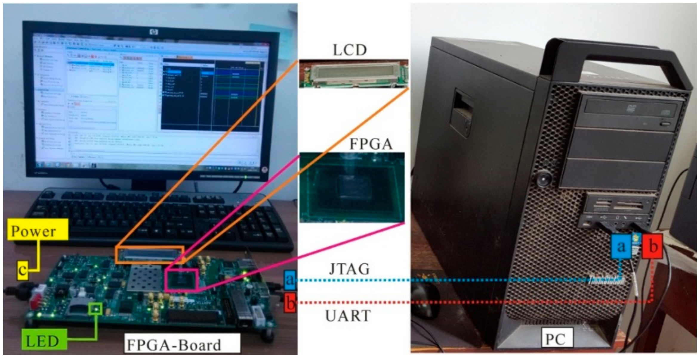
The hardware platform used in this paper is the AC701 Evaluation Kit of Artix-7 series produced by the Xilinx company (2100 Logic Drive, San Jose, CA 95124-3400, USA). The version of the FPGA is Xilinx Artix-7 XC7A200T FBG676ACX1349 D4658436A ZC. The design tool is ISE 4.7 and System Generator. The simulation tool is ModelSim SE10.1a. As shown in Figure 11, the FPGA Evaluation Kit uses the UART and JTAG ports to connect with the computer. The power port provides 250 V. The LCD (liquid crystal display) panel and the screen show the results at the same time. To validate the proposed method, the ortho-rectification algorithm is also implemented using Matlab 2015a (MathWorks, 1 Apple Hill Drive, Natick, MA 01760-2098, USA) on PC with a Windows 7 (64 bit) operation system, which is equipped with an Intel(R) Core(TM) i7-4790 CPU @ 3.6GHz (Intel company, 2200 Mission College Blvd, Santa Clara, CA 95054-1549, USA) and 8 GB RAM.
3.2. Data
To validate the proposed system based on an FPGA, two test data sets are used to perform the ortho-rectification. The first study area is located in central Denver, Colorado. The exploited aerial image (17,054 × 17,054), see Figure 12a, was collected on 17 April 2000 using an RC 30 aerial camera, which is the same as Zhou et al. [34]. The focal length is 153.022 mm and the flying height is 1650 m above the mean ground elevation of the imaged area. The second data set is acquired from an ERDAS IMAGINE example dataset, i.e., ps_napp.img (2294 × 2294) and ps_dem.img (see Figure 13). The known parameters, provided by the vendors, are listed in Table 1.
As described in part (2) of Section 2.2.2, to obtain the scanning coordinates, the affine transformation coefficients must be solved. To this end, four fiducial points for each study area are used to acquire the affine transformation coefficients according to Equation (16), and they are shown in Table 2.
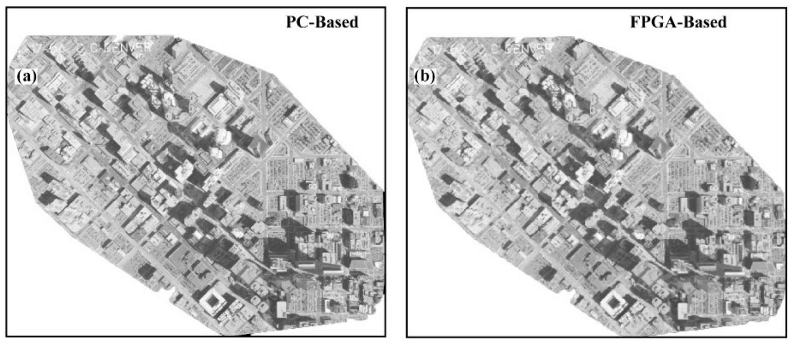
After the above necessary parameters are acquired, they are taken as the constants and input to the proposed FPGA-based ortho-rectification system. The ortho-rectified results (ortho-photo) using the proposed FPGA-based method are shown in Figure 14b and Figure 15b. To validate the rectification’s accuracy and speed, ortho-rectification for the same data sets was also implemented using the PC-based platform. The ortho-rectification results using the PC-based software are shown in Figure 14a and Figure 15a.
4. Discussion
4.1. Visual Check
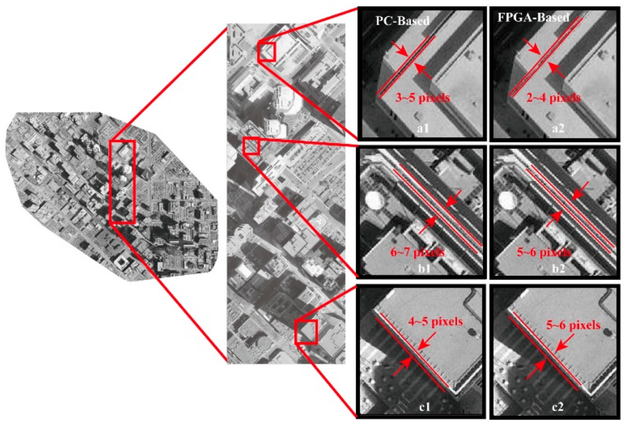
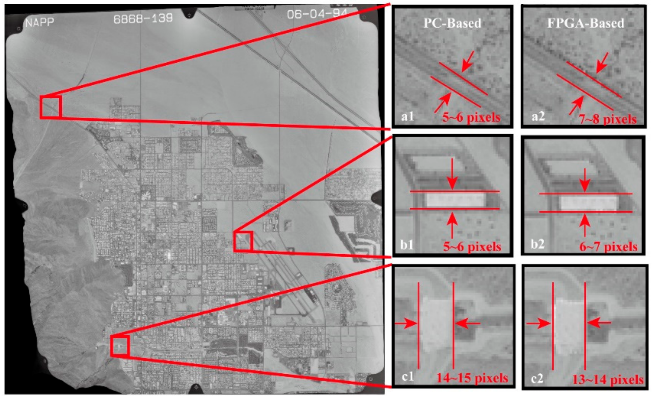
To validate the rectified accuracy, the ortho-photo results ortho-rectified by a PC-based platform are taken as the references. In each of the study areas, three sub-areas are chosen and zoomed into to visually check the accuracy (see Figure 16 and Figure 17). As observed from Figure 16 and Figure 17, the ortho-photos ortho-rectified by the proposed method expose one pixel’s difference when compared to the results from the PC-based platform. Through the visual check, it can be concluded that the proposed method can meet the demand of ortho-rectification in practice.
4.2. Error Analysis
To further quantitatively evaluate the ortho-photo accuracy obtained by the proposed method, the root-mean-square error (RMSE) [35,36] is applied to quantitatively analyze the rectification error of the proposed method. The RMSEs of the planimetric coordinates along the x- and y-axes, and distance (, and ), are computed by, respectively
where X′k and Y′k are the geodetic coordinates rectified by the proposed method; Xk and Yk are the reference geodetic coordinates; and n is the number of check points.
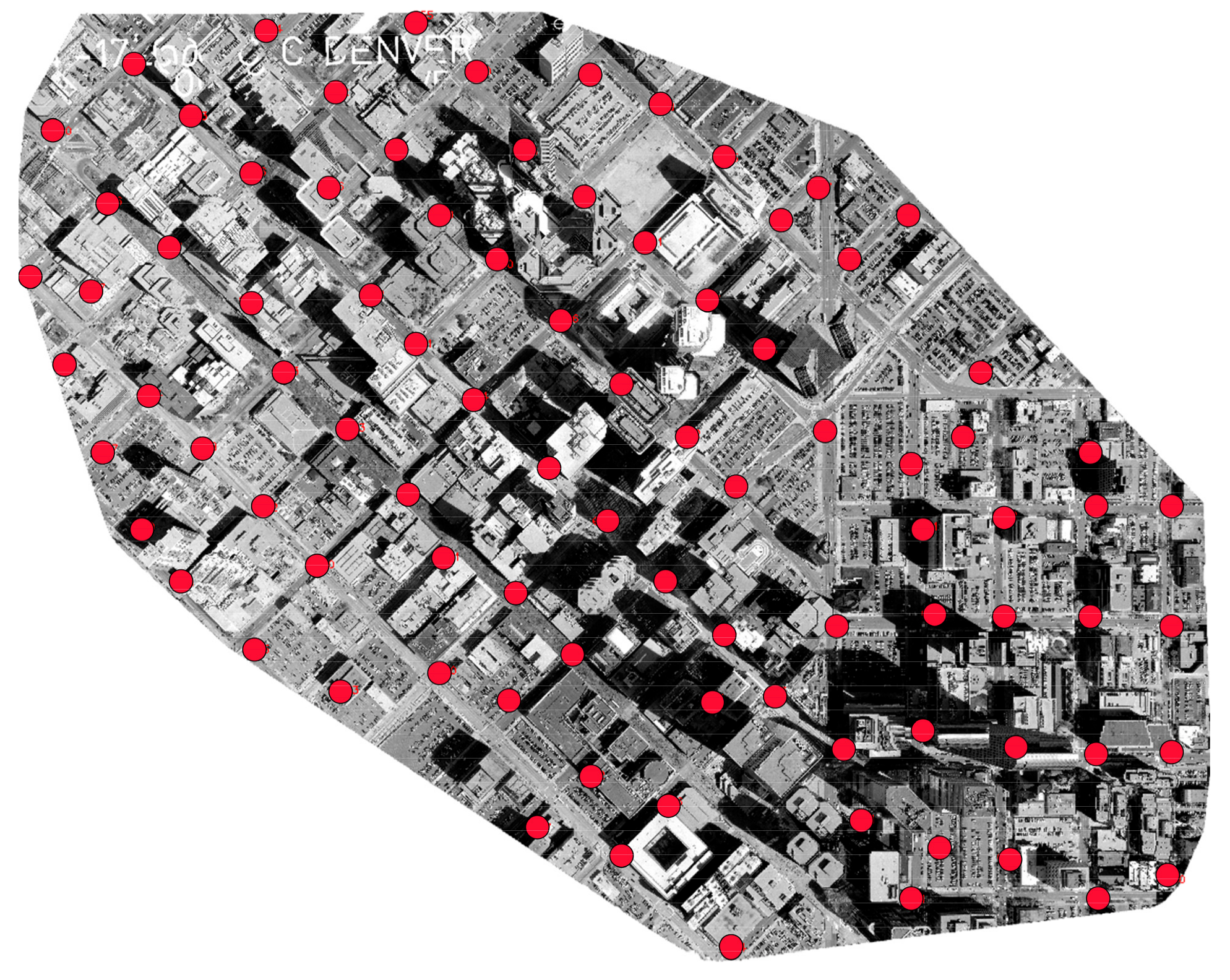
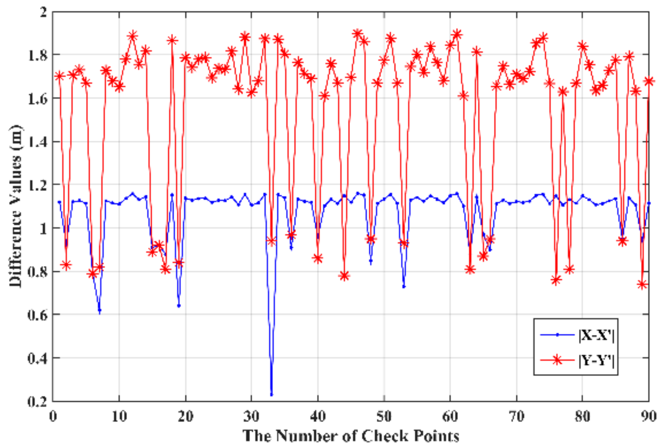
To this end, ninety check points (see Figure 18) for the first study area were selected to validate the accuracy achieved by the proposed method. The differences of coordinates obtained between the proposed method and the PC-based platform are shown in Figure 19. According to Equations (24)–(26) and Figure 19, the RMSEs of , and are 1.09 m, 1.61 m, and 1.93 m, respectively. In addition, other statistics, such as maximum value, minimum value, standard deviation, and mean of difference value are also computed and shown in Table 3. As shown in Table 3, the standard deviations of X and Y are very small. From Table 3, it can be found that the maximum error of the X and Y coordinates are 1.16 m and 1.89 m, respectively, and the standard deviation of the X and Y coordinates are 0.14 m and 0.38 m, respectively. According to Zhang et al. [37], the ultimate purpose of RS image rectification is to produce thematic maps from the rectified images. Whether the rectified images can satisfy the cartographic requirement of thematic maps depends on the scale of thematic maps. Because the minimum resolving distance on any map is only 0.1 mm, the tolerable errors on the ground distance vary with the scales of thematic maps. The tolerable error would be equivalent of 10 m on the ground if the scale of thematic map is 1:100,000. Because the rectification error obtained by the proposed method ranges from ~1 m to ~2 m, thus, the correction accuracy level of the proposed FPGA-based platform is suitable for compiling 1:10,000 to 1:20,000 thematic maps.
However, it is also noted that differences between the proposed method and the PC-based platform in the X and Y coordinates still exist. The difference may be caused by the algorithms implemented through the FPGA hardware, such as fix-point computation, which propagate and accumulate. In addition, the proposed FPGA-based platform only applies two octaves, while the PC-based platform applied at least eight octaves.
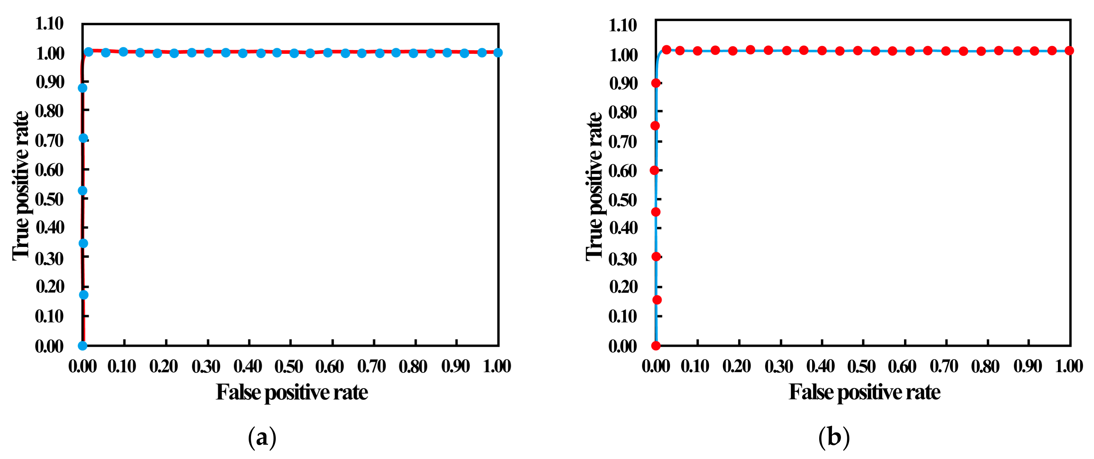
Moreover, another method (i.e., receiver operating characteristics curve, ROC curve) is used to evaluate the error of the proposed method. The ROC curve is useful for organizing classifiers and visualizing the performance of classifiers. The detailed information of the ROC curve can be found in [38]. In an ROC graph, the vertical axis represents the true positive rate (TPR) acquired by Equation (27) and the abscissa axis is the false positive rate (FPR) obtained by Equation (28). Let the difference of X-coordinate and Y-coordinates, which are less than 1 m, be of a positive class, and the others be of a negative class. Then, the differences are sorted by descending order. Finally, three differences of X-coordinates (the same as Y-coordinates) are used as a group to calculate the TPR and FPR. The ROC curves of the X-coordinates and Y-coordinates are shown in Figure 20a,b, respectively. As shown in Figure 20, there are 17 X-coordinates and 20 Y-coordinates that are less than 1 m. The ROC curve of the X-coordinates point at (0.013, 1) produces the highest TPR. Additionally, the ROC curve of the Y-coordinates point at (0.014, 1) produces the highest TPR.
4.3. Processing Speed Comparison
One of the most importance factors on on-board ortho-rectification is the processing speed. To evaluate and compare the speed of the proposed method and the PC-based platform, a normalized metric, i.e., throughput representing the capacity of processing pixels per second, is used. For the proposed FPGA-based platform, the throughput is 11,182.3 kilopixels per second and the whole time of the ortho-rectification processing is 26.01 s for the first study area. However, for the PC platform, the throughput is 2582.9 kilopixels per second and the total time of the ortho-rectification processing is 112.6 s for the same image. That means the processing speed by the proposed FPGA-based platform is approximately 4.3 times faster than that by the PC-based platform.
4.4. Resource Consumption
In addition, this paper takes the utilization ratio of each type of resource, such as input buffers (IBUF), output buffers (OBUF), and signal processors (DSP48E) to assess the proposed method.
First, the utilization ratios for the resources of the coordinate transformation module and the bilinear interpolation module are analyzed, independently. For implementing the coordinate transformation module of the proposed FPGA-based platform, the main hardware consists of 192 IBUF, 870 OBUF, and 78 DSP48E, as well as a few adding units (ADDSUB), multiplier units (MULT), and lookup tables (LUT). The results of the utilization ratios of the logic unit for implementing the coordinate transformation module are shown in Table 4.
For the bilinear interpolation module of the proposed FPGA-based platform, 129 slice resources, 291 IOs (inputs and outputs), and 75,779 LUTs are used. The utilization ratio of the IOs can reach 72% (291/400 ≈ 0.72). Additionally, the utilization ratio of LUT is 56% (75,779/134,600 ≈ 0.56) (see Table 5).
Generally, if the utilization ratio of a resource reaches 60–80%, it shows that the selected device can meet the requirements of the design scheme. If the utilization ratio of a resource is too low, it demonstrates that the selected device is wasted for implementing the design scheme. As shown in Table 4 and Table 5, the utilization ratios of register used in the coordinate transformation module and the bilinear interpolation module are only 34% and 24%, respectively. The utilization ratio of the register is relatively low in both models. The utilization ratios LUT applied in these two models are 27% and 56%, respectively. The utilization ratio of LUT used in the bilinear interpolation module is about twice higher than the utilization ratio of LUT applied in the coordinate transformation module. The reason is that the bilinear interpolation module needs to store the gray values of neighbors. Additionally, the utilization ratios of the Flip Flop and control sets are low in both models. Moreover, the utilization ratios of LUT–FF pairs, IOs and IOBs (input output blocks) are relatively high in both models. In summary, according to the above comprehensive utilization ratios for resources, it can be demonstrated that the resources of the selected FPGA can meet the design requirement of the proposed FPGA-based ortho-rectification method.
5. Conclusions
In this paper, an FPGA-based ortho-rectification method, which is intended to perform the ortho-rectification process on board spacecraft, is proposed for accelerating the speed of the ortho-rectification of remotely sensed images. The proposed FPGA-based ortho-rectification platform consists of a memory module, a coordinate transformation module (including the transformation from geodetic to photo coordinates and the transformation from photo to scanning coordinates), and a gray-scale interpolation module based on a bilinear interpolation algorithm.
To validate the ortho-rectification’s accuracy, an ortho-photo ortho-rectified by a PC-based platform is taken as a reference. Two study areas, including three subareas, are chosen to validate the proposed method. The root-mean-square error (RMSE), associated with maximum, minimum, standard deviation, and mean of the X and Y coordinates’ differences are used. The experimental results demonstrated that the maximum errors of the X and Y coordinates are 1.16 m and 1.89 m, respectively, and the standard deviations of the X and Y coordinates are 0.14 m and 0.38 m, respectively. The RMSEs of the planimetric coordinates along the X- and Y-axes (φX, φY) and the distance φS are 1.09 m, 1.61 m, and 1.93 m, respectively. Thereby, it can be concluded from these quantitative analyses that the proposed method can meet the demand of ortho-rectification in practice.
In addition, through analyzing the processing speed of ortho-rectification, it can be found that the processing speed by the proposed FPGA-based platform is approximately 4.3 times faster than that by the PC-based platform. In terms of the resource consumptions, it can found that the bilinear interpolation module of the proposed method utilizes 129 slice resources and 291 IOs, whose utilization ratio of the IOs can reach 72%, and the LUT achieves 56%.
Acknowledgments
This paper is financially supported by the National Natural Science of China under Grant numbers 41431179 and 41162011, The National Key Research and Development Program of China under Grant numbers 2016YFB0502501 and The State Oceanic Administration under Grant numbers [2014]#58, GuangXi Natural Science Foundation under grant numbers 2015GXNSFDA139032, and 2012GXNSFCB05300; Guangxi Science & Technology Development Program under the Contract number GuiKeHe 14123001-4, and GuangXi Key Laboratory of Spatial Information and Geomatics Program (Contract No. GuiKeNeng110310801, 120711501, and 130511401, 140452401, 140452409, 151400701, 151400712, 151400716, 163802506, and 163802530), the “BaGuiScholars” program of the provincial government of Guangxi.
Author Contributions
G. Zhou conceived and designed the experiments. R. Zhang performed the experiments and wrote the initial paper. N. Liu conducted the experiments, and J. Huang analyzed the data. X. Zhou drawn and improved the illustration.
Conflicts of Interest
The authors declare no conflict of interest.
References
- Pan, Z.; Lei, J.; Zhang, Y.; Sun, X.; Kwong, S. Fast motion estimation based on content property for low-complexity H.265/HEVC encoder. IEEE Trans. Broadcast. 2016, 62, 675–684. [Google Scholar] [CrossRef]
- Jiang, C.; Nooshabadi, S. A scalable massively parallel motion and disparity estimation scheme for multiview video coding. IEEE Trans. Circuits Syst. Video Technol. 2016, 26, 346–359. [Google Scholar] [CrossRef]
- Warpenburg, M.R.; Siegel, L.J. SIMD image resampling. IEEE Trans. Comput. 1982, 31, 934–942. [Google Scholar] [CrossRef]
- Wittenbrink, C.M.; Somani, A.K. 2D and 3D optimal parallel image warping. J. Parallel Distrib. Comput. 1995, 25, 197–208. [Google Scholar] [CrossRef]
- Sylvain, C.V.; Serge, M. A load-balanced algorithm for parallel digital image warping. Int. J. Pattern Recognit. Artif. Intell. 1999, 13, 445–463. [Google Scholar]
- Dai, C.; Yang, J. Research on orthorectification of remote sensing images using GPU-CPU cooperative processing. In Proceedings of the International Symposium on Image and Data Fusion, Tengchong, China, 9–11 August 2011; pp. 1–4. [Google Scholar]
- Escamilla-Hernández, E.; Kravchenko, V.; Ponomaryov, V.; Robles-Camarillo, D.; Ramos, L.E. Real time signal compression in radar using FPGA. Científica 2008, 12, 131–138. [Google Scholar]
- Kate, D. Hardware implementation of the huffman encoder for data compression using altera DE2 board. Int. J. Adv. Eng. Sci. 2012, 2, 11–15. [Google Scholar]
- Pal, C.; Kotal, A.; Samanta, A.; Chakrabarti, A.; Ghosh, R. An efficient FPGA implementation of optimized anisotropic diffusion filtering of images. Int. J. Reconfig. Comput. 2016, 2016, 1. [Google Scholar] [CrossRef]
- Wang, E.; Yang, F.; Tong, G.; Qu, P.; Pang, T. Particle filtering approach for gnss receiver autonomous integrity monitoring and FPGA implementation. Telecommun. Comput. Electron. Control 2016, 14. [Google Scholar] [CrossRef]
- Zhang, C.; Liang, T.; Mok, P.K.T.; Yu, W. FPGA implementation of the coupled filtering method. In Proceedings of the 2016 IEEE International Conference on Bioinformatics and Biomedicine (BIBM), Shenzhen, China, 15–18 December 2016; pp. 435–442. [Google Scholar]
- Ontiveros-Robles, E.; Vázquez, J.G.; Castro, J.R.; Castillo, O. A FPGA-based hardware architecture approach for real-time fuzzy edge detection. Nat. Inspired Des. Hybrid Intell.Syst. 2017, 667, 519–540. [Google Scholar]
- Ontiveros-Robles, E.; Gonzalez-Vazquez, J.L.; Castro, J.R.; Castillo, O. A hardware architecture for real-time edge detection based on interval type-2 fuzzy logic. In Proceedings of the IEEE International Conference on Fuzzy Systems, Vancouver, BC, Canada, 24–29 July 2016. [Google Scholar]
- Li, H.H.; Liu, S.; Piao, Y. Snow removal of video image based on FPGA. In Proceedings of the 5th International Conference on Electrical Engineering and Automatic Control, Weihai, China, 16–18 October 2015; Huang, B., Yao, Y., Eds.; Springer: Berlin/Heidelberg, Germany, 2016; pp. 207–215. [Google Scholar]
- Li, H.; Xiang, F.; Sun, L. Based on the FPGA video image enhancement system implementation. DEStech Trans. Comput. Sci. Eng. 2016. [Google Scholar] [CrossRef]
- González, D.; Botella, G.; Meyer-Baese, U.; García, C.; Sanz, C.; Prieto-Matías, M. A low cost matching motion estimation sensor based on the NIOS II microprocessor. Sensors 2012, 12, 13126–13149. [Google Scholar] [CrossRef] [PubMed] [Green Version]
- González, D.; Botella, G.; García, C.; Prieto, M.; Tirado, F. Acceleration of block-matching algorithms using a custom instruction-based paradigm on a NIOS II microprocessor. EURASIP J. Adv. Signal Proc. 2013, 2013, 118. [Google Scholar] [CrossRef] [Green Version]
- Botella, G.; Garcia, A.; Rodriguez-Alvarez, M.; Ros, E.; Meyer-Baese, U.; Molina, M.C. Robust bioinspired architecture for optical-flow computation. IEEE Trans. VLSI Syst. 2010, 18, 616–629. [Google Scholar] [CrossRef]
- Waidyasooriya, H.; Hariyama, M.; Ohtera, Y. FPGA architecture for 3-D FDTD acceleration using open CL. In Proceedings of the 2016 Progress in Electromagnetic Research Symposium (PIERS), Shanghai, China, 8–11 August 2016; p. 4719. [Google Scholar]
- Rodriguez-Donate, C.; Botella, G.; Garcia, C.; Cabal-Yepez, E.; Prieto-Matias, M. Early experiences with OpenCL on FPGAs: Convolution case study. In Proceedings of the 2015 IEEE 23rd Annual International Symposium on Field-Programmable Custom Computing Machines, Vancouver, BC, Canada, 2–6 May 2015; p. 235. [Google Scholar]
- Thomas, U.; Rosenbaum, D.; Kurz, F.; Suri, S.; Reinartz, P. A new software/hardware architecture for real time image processing of wide area airborne camera images. J. Real-Time Image Proc. 2008, 4, 229–244. [Google Scholar] [CrossRef]
- Kalomiros, J.A.; Lygouras, J. Design and evaluation of a hardware/software FPGA-based system for fast image processing. Microproc. Microsyst. 2008, 32, 95–106. [Google Scholar] [CrossRef]
- Kuo, D.; Gordon, D. Real-time orthorectification by FPGA-based hardware acceleration. In Remote Sensing; International Society for Optics and Photonics: Bellingham, WA, USA, 2010; p. 78300Y. [Google Scholar]
- Halle, W. Thematic data processing on board the satellite BIRD. In Proceedings of the SPIE 4540, Sensors, Systems, and Next-Generation Satellites V, Toulouse, France, 17–20 September 2001. [Google Scholar]
- Malik, A.W.; Thornberg, B.; Imran, M.; Lawal, N. Hardware architecture for real-time computation of image component feature descriptors on a FPGA. Int. J. Distrib. Sens. Netw. 2014, 2014, 14. [Google Scholar] [CrossRef]
- Tomasi, M.; Vanegas, M.; Barranco, F.; Diaz, J.; Ros, E. Real-time architecture for a robust multi-scale stereo engine on FPGA. IEEE Trans. Very Large Scale Integr. Syst. 2012, 20, 2208–2219. [Google Scholar] [CrossRef]
- Greisen, P.; Heinzle, S.; Gross, M.; Burg, A.P. An FPGA-based processing pipeline for high-definition stereo video. EURASIP J. Image Video Proc. 2011, 2011, 1–13. [Google Scholar] [CrossRef]
- Kumar, P.R.; Sridharan, K. VLSI-efficient scheme and FPGA realization for robotic mapping in a dynamic environment. IEEE Trans. Very Large Scale Integr. Syst. 2007, 15, 118–123. [Google Scholar] [CrossRef]
- Hsiao, P.Y.; Lu, C.L.; Fu, L.C. Multilayered image processing for multiscale harris corner detection in digital realization. IEEE Trans. Ind. Electron. 2010, 57, 1799–1805. [Google Scholar] [CrossRef]
- Kazmi, M.; Aziz, A.; Akhtar, P. An efficient and compact row buffer architecture on FPGA for real-time neighbourhood image processing. J. Real-Time Image Proc. 2017. [Google Scholar] [CrossRef]
- Cao, T.P.; Elton, D.; Deng, G. Fast buffering for FPGA implementation of vision-based object recognition systems. J. Real-Time Image Proc. 2012, 7, 173–183. [Google Scholar] [CrossRef]
- Hu, X.; Zhu, Y. Research on FPGA based image input buffer design mechanism. Microcomput. Inform. 2010, 26, 5–6. [Google Scholar]
- El-Amawy, A. A systolic architecture for fast dense matrix inversion. IEEE Trans. Comput. 1989, 38, 449–455. [Google Scholar] [CrossRef]
- Zhou, G.; Chen, W.; Kelmelis, J.A.; Zhang, D. A comprehensive study on urban true orthorectification. IEEE Trans. Geosci. Remote Sens. 2005, 43, 2138–2147. [Google Scholar] [CrossRef]
- Shi, W.; Shaker, A. Analysis of terrain elevation effects on IKONOS imagery rectification accuracy by using non-rigorous models. Photogramm. Eng. Remote Sens. 2003, 69, 1359–1366. [Google Scholar] [CrossRef]
- Reinartz, P.; Müller, R.; Lehner, M.; Schroeder, M. Accuracy analysis for DSM and orthoimages derived from SPOT HRS stereo data using direct georeferencing. ISPRS J. Photogramm. Remote Sens. 2006, 60, 160–169. [Google Scholar] [CrossRef]
- Zhang, Y.; Zhang, D.; Gu, Y.; Tao, F. Impact of GCP distribution on the rectification accuracy of Landsat TM imagery in a coastal zone. ACTA Oceanol. Sin Engl. Ed. 2006, 25, 14. [Google Scholar]
- Fawcett, T. An introduction to ROC analysis. Pattern Recognit. Lett. 2006, 27, 861–874. [Google Scholar] [CrossRef]
Figure 1.
The proposed field programmable gate array (FPGA)-based architecture for the ortho-rectification of remotely sensed (RS) images. RAM, random access memory. CLK, clock. RSTn, reset. EN, enable.
Figure 1.
The proposed field programmable gate array (FPGA)-based architecture for the ortho-rectification of remotely sensed (RS) images. RAM, random access memory. CLK, clock. RSTn, reset. EN, enable.

Figure 2.
State diagram of cache for image input [32]. IDEL, initialization.
Figure 2.
State diagram of cache for image input [32]. IDEL, initialization.

Figure 3.
The model of the two-row buffer.

Figure 4.
FPGA-based parallel computation architecture for calculating geodetic coordinates Xg, Yg, and Zg.
Figure 4.
FPGA-based parallel computation architecture for calculating geodetic coordinates Xg, Yg, and Zg.

Figure 5.
(a) FPGA-based computation for elements of rotation matrix R; (b) The FPGA implementation architecture for coordinate transformation from geodetic to photo coordinates.
Figure 5.
(a) FPGA-based computation for elements of rotation matrix R; (b) The FPGA implementation architecture for coordinate transformation from geodetic to photo coordinates.
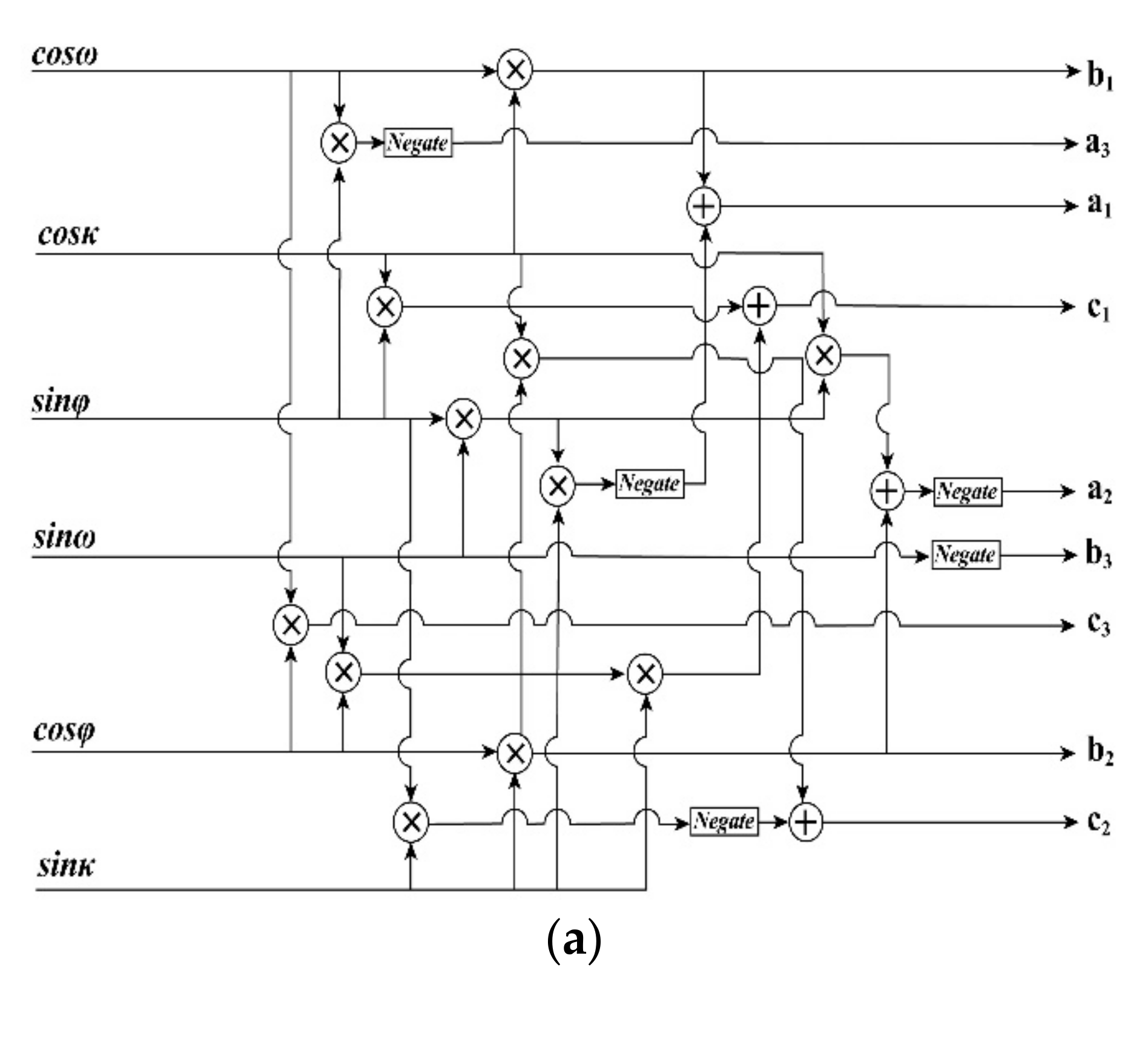

Figure 6.
The FPGA implementation architecture of QTQ.

Figure 7.
The FPGA-based architecture for calculating lij and dii.
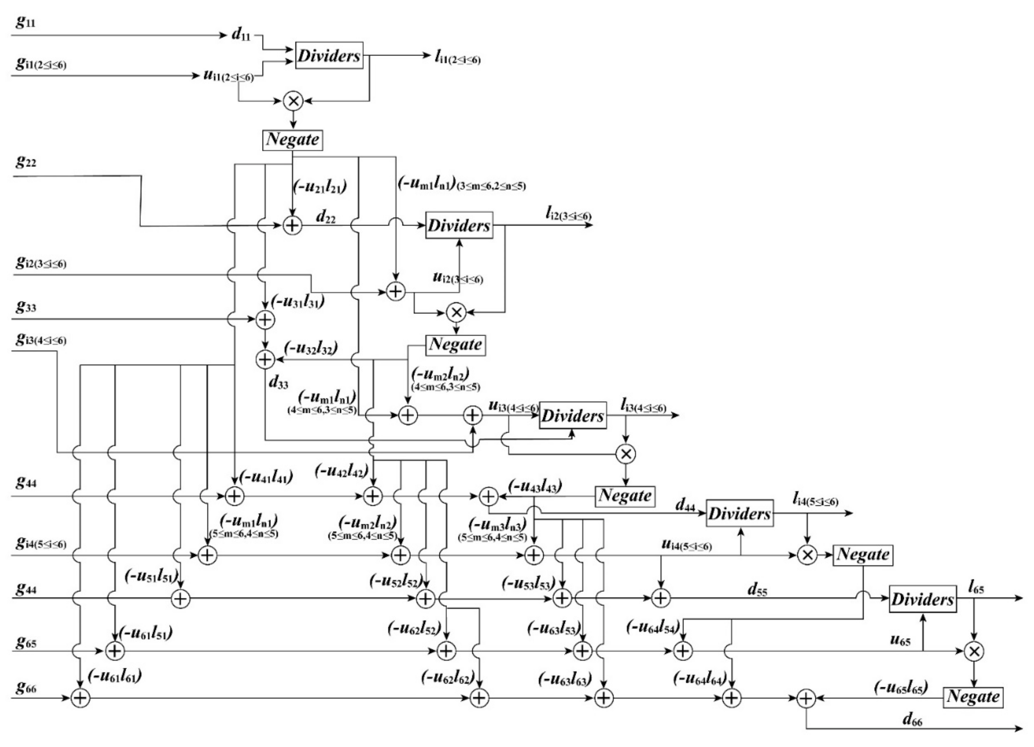
Figure 8.
The FPGA-based architecture for the inversion of G. MUX, multiplex module.
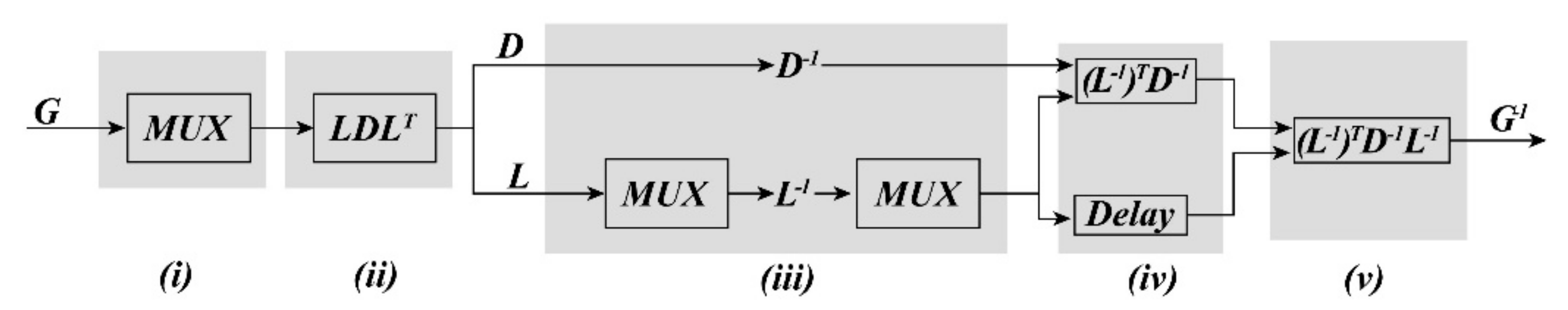
Figure 9.
The FPGA-based architecture for the transformation from photo coordinates to scanning coordinates.
Figure 9.
The FPGA-based architecture for the transformation from photo coordinates to scanning coordinates.

Figure 10.
The FPGA implementation architecture for the bilinear interpolation algorithm. INT, integerize.
Figure 10.
The FPGA implementation architecture for the bilinear interpolation algorithm. INT, integerize.

Figure 11.
System diagram. LCD, liquid crystal display. LED, light-emitting diode. PC, personal computer.
Figure 11.
System diagram. LCD, liquid crystal display. LED, light-emitting diode. PC, personal computer.

Figure 12.
(a) The original aerial image covering the first study area; (b) digital surface model (DSM) covering the first study area (Zhou et al. [34]).
Figure 12.
(a) The original aerial image covering the first study area; (b) digital surface model (DSM) covering the first study area (Zhou et al. [34]).
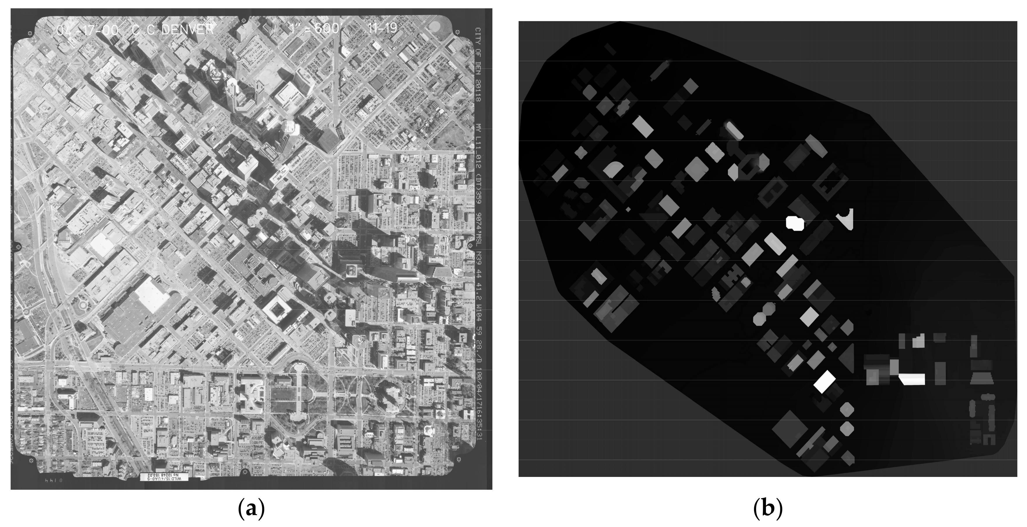
Figure 13.
(a) The original aerial image covering the second study area; (b) digital elevation model (DEM) covering the second study area (from ERDAS IMAGINE 9.2).
Figure 13.
(a) The original aerial image covering the second study area; (b) digital elevation model (DEM) covering the second study area (from ERDAS IMAGINE 9.2).
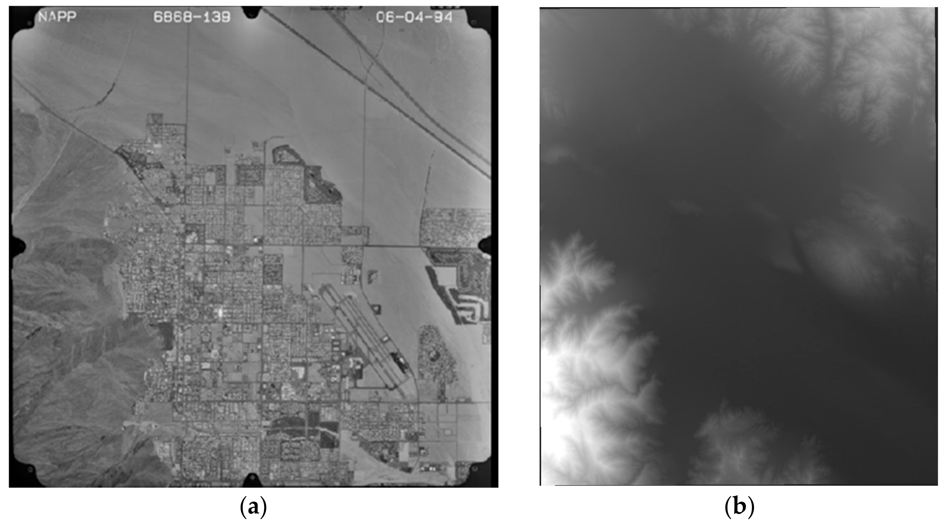
Figure 14.
The ortho-photo ortho-rectified by (a) the personal computer (PC)-based platform; (b) and the proposed method in the first study area.
Figure 14.
The ortho-photo ortho-rectified by (a) the personal computer (PC)-based platform; (b) and the proposed method in the first study area.

Figure 15.
The ortho-photo ortho-rectified by (a) the PC-based platform; (b) and the proposed method in the second study area.
Figure 15.
The ortho-photo ortho-rectified by (a) the PC-based platform; (b) and the proposed method in the second study area.
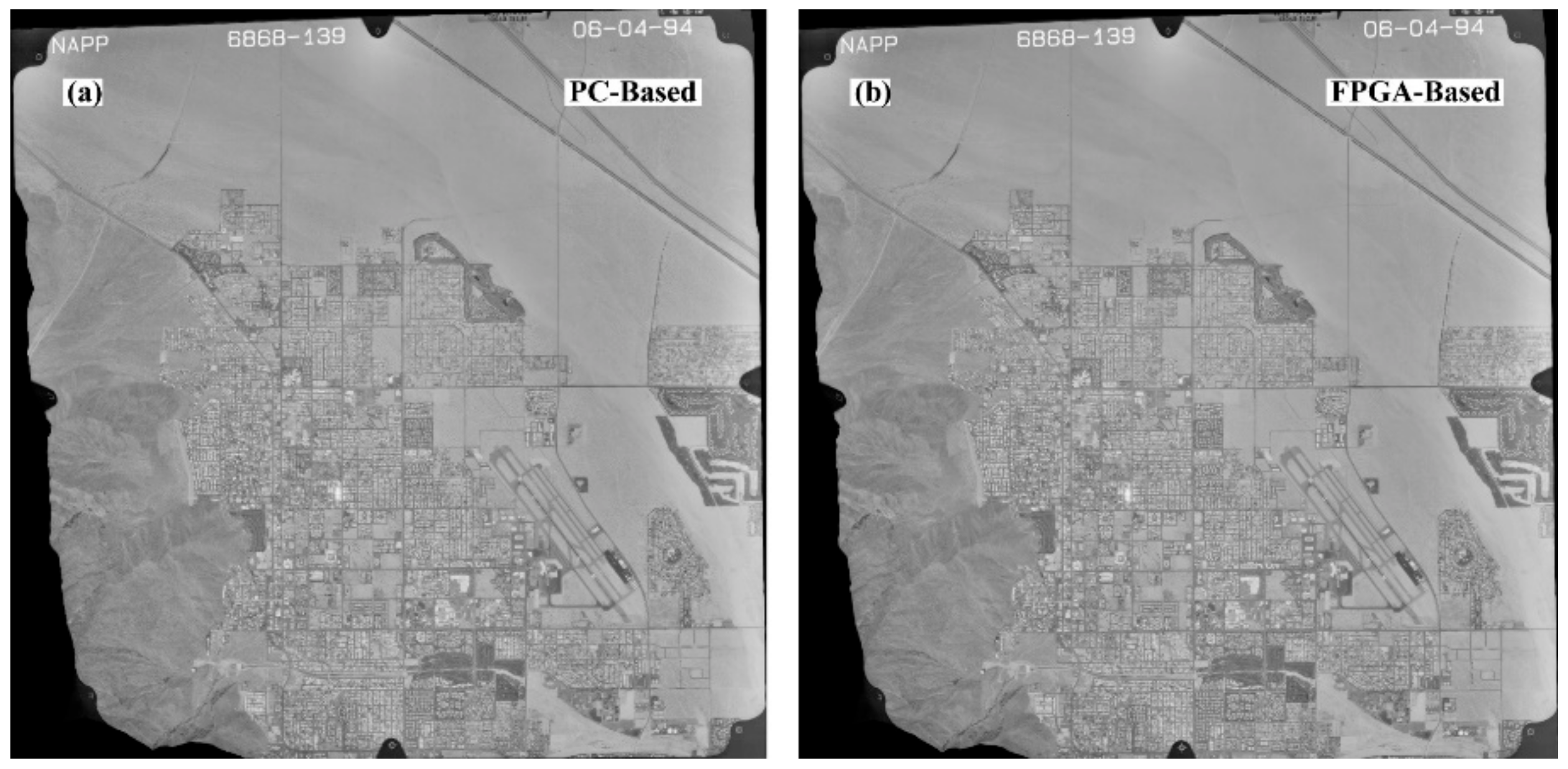
Figure 16.
Visual check analysis for the ortho-rectified results in the three subareas of the first study area.
Figure 16.
Visual check analysis for the ortho-rectified results in the three subareas of the first study area.

Figure 17.
Visual check analysis for the ortho-rectified results in the three subareas of the second study area.
Figure 17.
Visual check analysis for the ortho-rectified results in the three subareas of the second study area.

Figure 18.
The distribution of the 90 check points labeled as red in the first study area.

Figure 19.
Different statistics analysis for ortho-photos obtained by our method and the PC-based platform.
Figure 19.
Different statistics analysis for ortho-photos obtained by our method and the PC-based platform.

Figure 20.
The receiver operating characteristics (ROC) curve analysis through the difference of the X-coordinates (a) and Y-coordinates (b).
Figure 20.
The receiver operating characteristics (ROC) curve analysis through the difference of the X-coordinates (a) and Y-coordinates (b).


Table 1.
The known parameters for the data sets of the two study areas.
| Known Parameters | First Study Area | Second Study Area |
|---|---|---|
| x0 | 0.002 | −0.004 |
| y0 | −0.004 | 0.000 |
| f (mm) | 153.022 | 152.8204 |
| XS (m) | 3,143,040.5560 | 543,427.1886 |
| YS (m) | 1,696,520.9258 | 3,744,740.3247 |
| ZS (m) | 9072.2729 | 6743.2730 |
| ω (rad) | −0.02985539 | 0.63985182 |
| φ (rad) | −0.00160606 | −0.65999005 |
| κ (rad) | −1.55385318 | 0.86709830 |
Table 2.
Four fiducial points for each study area.
| # | The First Study Area | The Second Study Area | ||||||
|---|---|---|---|---|---|---|---|---|
| i | j | u | v | i | j | u | v | |
| FP1 | 683.403 | 881.001 | −196.100 | 191.150 | 87.500 | 88.501 | −106.000 | 106.000 |
| FP2 | 15,820.521 | 835.103 | 182.325 | 192.300 | 2208.499 | 83.501 | 105.999 | 105.994 |
| FP3 | 15,868.602 | 15,970.971 | 183.525 | −186.075 | 2213.503 | 2204.504 | 105.998 | −105.999 |
| FP4 | 730.452 | 16,019.980 | −194.925 | −187.300 | 92.500 | 2209.501 | −106.008 | −105.998 |
Table 3.
Statistics of difference value of geodetic coordinate.
| # | Max | Min | Mean | Standard Deviation |
|---|---|---|---|---|
| X coordinates | 1.16 m | 0.23 m | 1.07 m | 0.14 m |
| Y coordinates | 1.89 m | 0.74 m | 1.55 m | 0.38 m |
Table 4.
The utilization ratios of logic units for the coordinate transformation module. LUT, Look Up Table; FF, Flip Flop; IOB, Input output block.
Table 4.
The utilization ratios of logic units for the coordinate transformation module. LUT, Look Up Table; FF, Flip Flop; IOB, Input output block.
| # | Name of Logic Unit | Utilization Ratio (%) |
|---|---|---|
| Logic unit resource | Register | 34 |
| Distribution of logic unit | Flip Flop | 12 |
| LUT | 27 | |
| LUT-FF Pairs | 58 | |
| Control Sets | 2 | |
| Input and output (IO) | IOs | 78 |
| IOBs | 54 |
Table 5.
The utilization ratios of logic units for the bilinear interpolation module.
| # | Name of Logic Unit | Utilization Ratio (%) |
|---|---|---|
| Use ratio of logic unit | Register | 24 |
| Distribution of logic unit | Flip Flop | 17 |
| LUT | 56 | |
| LUT-FF Pairs | 64 | |
| Control Sets | 7 | |
| Input and output (IO) | IOs | 72 |
| IOBs | 65 |
© 2017 by the authors. Licensee MDPI, Basel, Switzerland. This article is an open access article distributed under the terms and conditions of the Creative Commons Attribution (CC BY) license (http://creativecommons.org/licenses/by/4.0/).
Share and Cite
MDPI and ACS Style
Zhou, G.Z.R.Z.N.L.J.H.a.X.; Zhang, R.; Liu, N.; Huang, J.; Zhou, X. On-Board Ortho-Rectification for Images Based on an FPGA. Remote Sens. 2017, 9, 874. https://doi.org/10.3390/rs9090874
AMA Style
Zhou GZRZNLJHaX, Zhang R, Liu N, Huang J, Zhou X. On-Board Ortho-Rectification for Images Based on an FPGA. Remote Sensing. 2017; 9(9):874. https://doi.org/10.3390/rs9090874
Chicago/Turabian StyleZhou, Guoqing Zhou Rongting Zhang Na Liu Jingjin Huang and Xiang, Rongting Zhang, Na Liu, Jingjin Huang, and Xiang Zhou. 2017. "On-Board Ortho-Rectification for Images Based on an FPGA" Remote Sensing 9, no. 9: 874. https://doi.org/10.3390/rs9090874
Note that from the first issue of 2016, this journal uses article numbers instead of page numbers. See further details here.