Article

Classification of Tree Species in a Diverse African Agroforestry Landscape Using Imaging Spectroscopy and Laser Scanning

1
Earth Change Observation Laboratory, Department of Geosciences and Geography, University of Helsinki, P.O. Box 64, FI-00014 Helsinki, Finland
2
Fisheries and Environmental Management Group, Department of Environmental Sciences, University of Helsinki, P.O. Box 68, FI-00014 Helsinki, Finland
3
Finnish Environmental Institute (SYKE), Environmental Policy Centre, P.O. Box 140, FI-00251 Helsinki, Finland
*
Author to whom correspondence should be addressed.
Remote Sens. 2017, 9(9), 875; https://doi.org/10.3390/rs9090875
Submission received: 14 July 2017 / Revised: 14 August 2017 / Accepted: 18 August 2017 / Published: 23 August 2017
(This article belongs to the Special Issue Hyperspectral Imaging and Applications)

Abstract

:
Airborne imaging spectroscopy (IS) and laser scanning (ALS) have been explored widely for tree species classification during the past decades. However, African agroforestry areas, where a few exotic tree species are dominant and many native species occur less frequently, have not yet been studied. Obtaining maps of tree species would provide useful information for the characterization of agroforestry systems and detecting invasive species. Our objective was to study tree species classification in a diverse tropical landscape using IS and ALS data at the tree crown level, with primary interest in the exotic tree species. We performed multiple analyses based on different IS and ALS feature sets, identified important features using feature selection, and evaluated the impact of combining the two data sources. Given that a high number of tree species with limited sample size (499 samples for 31 species) was expected to limit the classification accuracy, we tested different approaches to group the species based on the frequency of their occurrence and Jeffries–Matusita (JM) distance. Surface reflectance at wavelengths between 400–450 nm and 750–800 nm, and height to crown width ratio, were identified as important features. Nonetheless, a selection of minimum noise fraction (MNF) transformed reflectance bands showed superior performance. Support vector machine classifier performed slightly better than the random forest classifier, but the improvement was not statistically significant for the best performing feature set. The highest F1-scores were achieved when each of the species was classified separately against a mixed group of all other species, which makes this approach suitable for invasive species detection. Our results are valuable for organizations working on biodiversity conservation and improving agroforestry practices, as we showed how the non-native Eucalyptus spp., Acacia mearnsii and Grevillea robusta (mean F1-scores 76%, 79% and 89%, respectively) trees can be mapped with good accuracy. We also found a group of six fruit bearing trees using JM distance, which was classified with mean F1-score of 65%. This was a useful finding, as these species could not be classified with acceptable accuracy individually, while they all share common economic and ecological importance.

Graphical Abstract

1. Introduction

Globally, more than 55% of new agricultural land in tropics was converted from forests between 1980 and 2000 [1]. In eastern Africa, the yearly increase rate of agricultural land has been 1.4% during 1990–2010, while the yearly deforestation rate increased from 0.2% during 1990–2000 to 0.4% during 2000–2010 [2]. Agroforestry systems are considered as an option for mitigating the negative impacts of this change [3,4]. In addition, selecting proper tree species is important for a productive and environmentally sustainable agroforestry system [5,6,7]. However, the transformation of forests and woodlands into agroforestry might decrease biodiversity as native tree species are often replaced with exotic species. In the Afromontane highlands of the Taita Hills (southeast Kenya), 66.5% of tree species observed in the croplands (agroforestry) are exotic, and were associated in a recent study with functional traits such as economic function and nitrogen fixation [8].
Remote sensing based tree species mapping has great potential to reduce costs of observing changes in the tree species composition in comparison to field based approaches that require large number of field plots [9]. In their recent review, Fassnacht et al. [9] identified that common motives for tree species classification using remote sensing include biodiversity assessment and monitoring, monitoring of invasive species, hazard and stress management, wildlife habitat mapping, sustainable forest management, and resource inventory. Airborne laser scanning (ALS) and imaging spectroscopy (IS) were the most commonly used data types in the recent studies. Most studies had been conducted in temperate forests, while tropical forests had been studied in South America and savannah systems in South Africa [9]. The review did not list any studies from a diverse agroforestry landscape in Africa with patches of shrubland and native forest, where a few exotic tree species are dominant and a high number of native species occur less frequently. This leads to imbalance in the training data used in classification [10]. Although the cost of IS and ALS based tree species mapping is low in comparison to covering the study area on foot, airborne remote sensing is more expensive than satellite-based remote sensing data. However, mapping trees on species level with satellite-based data is challenging in agroforestry landscape, where trees are often isolated on farmland and high resolution data are needed to detect the trees at the crown level.
Previous studies with a high number of tree species have shown decline in the classification accuracy with the increasing number of classes [11], and increase in accuracy with the greater number of samples per species [12]. However, collecting comprehensive field reference data for all the species in a high species diversity system is challenging. The negative impact of imbalanced or limited training data on tree species classification has been approached, for example, by standardizing class sizes using down-sampling [10,13], and by using semi-supervised approaches to increase the size of training data from unlabeled observations [14]. However, we did not find studies where class sizes were balanced using up-sampling, or where different approaches to divide the species into groups based on their spectral and structural characteristics using Jeffries–Matusita (JM) distance, were compared.
According to Fassnacht et al. [9], non-parametric support vector machine (SVM) [15] and random forest (RF) [16] are the most commonly used classifiers for tree species classification. Both classifiers have performed well in remote sensing based classifications while neither has constantly outperformed the other [17,18,19]. Feature extraction and/or feature selection methods are commonly used with high dimensional data to improve the classification accuracy; in particular, the minimum noise fraction (MNF) transformation [20] has performed well in the previous studies [9,18,21].
The main aim of this study was to study tree species classification in an African agroforestry landscape with high species diversity and imbalanced training set. The specific objectives of the study were to:
  • compare the performance of the different feature sets derived from IS and ALS data using SVM and RF classifiers;
  • find species or groups of species with ecological or economical function that can be detected relatively accurately; and
  • evaluate the impact of up-sampling and different approaches to group the species on the classification accuracy.

2. Material and Methods
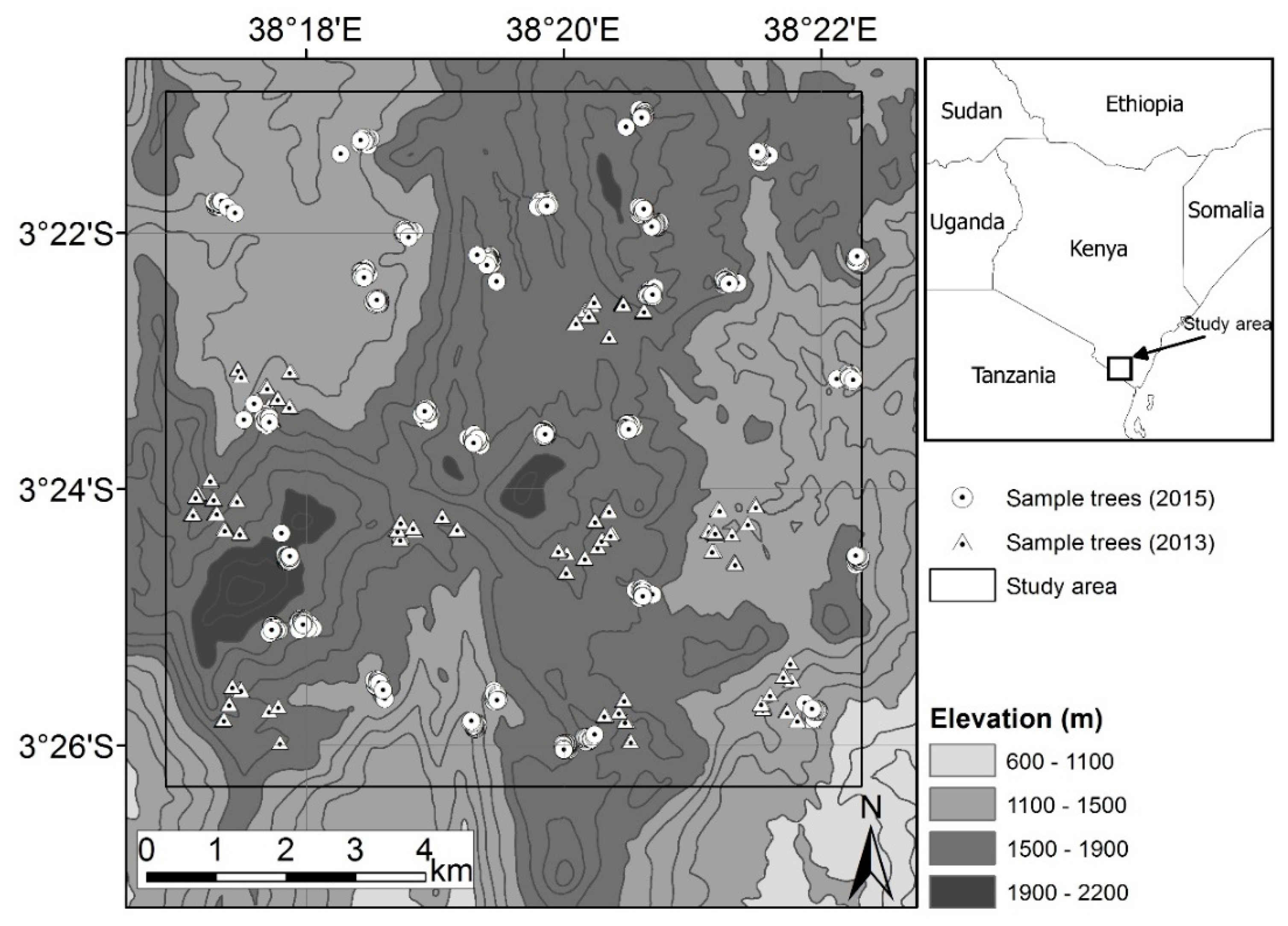
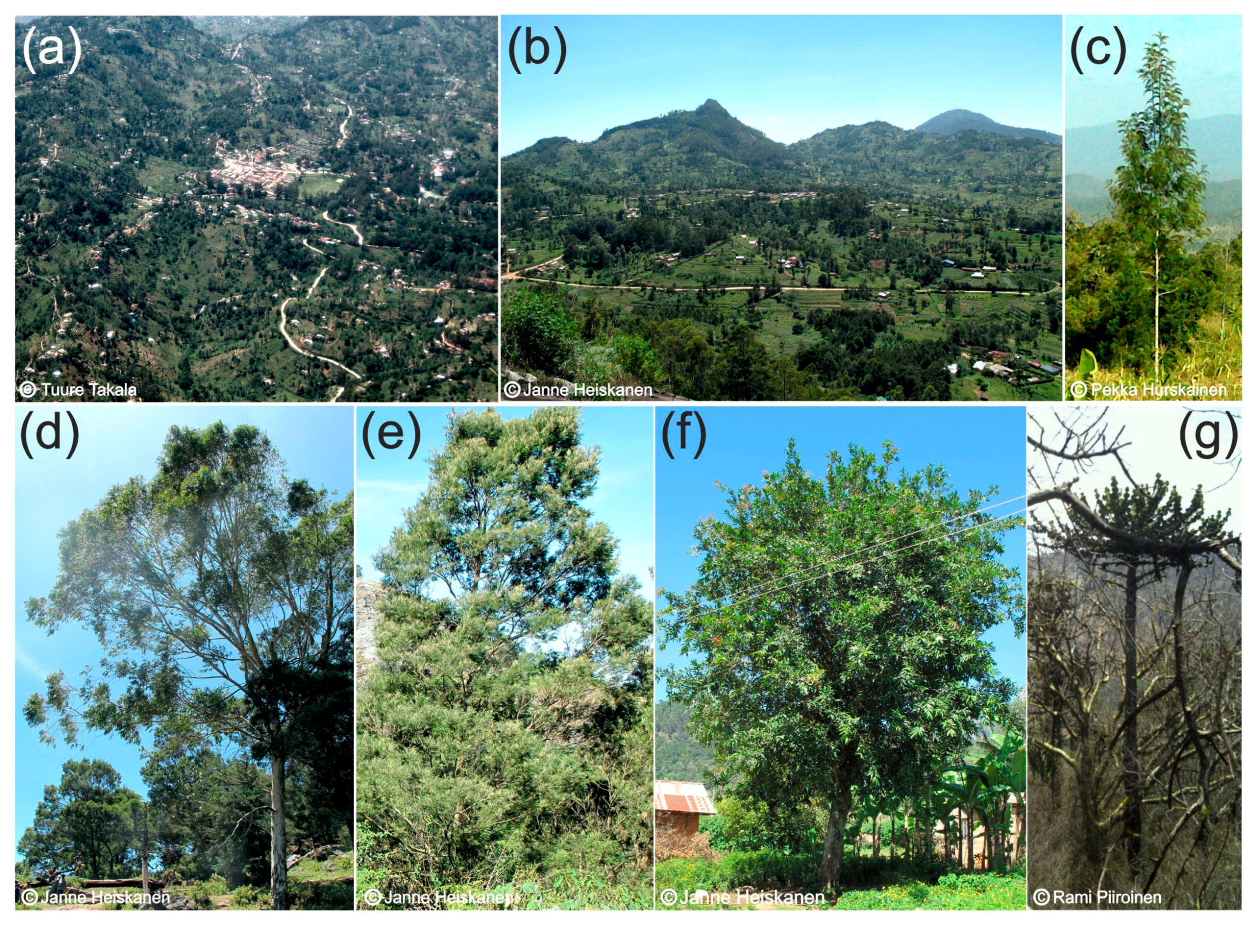
2.1. Study Site

The study area (10 km × 10 km) was located in the elevation range of 1100–2200 m a.s.l. in the Taita Hills (3°25′ S, 38°19′ E) in southeast Kenya (Figure 1). The Taita Hills are part of the Eastern Arc Mountains (EAM). There are two rainy seasons with long rains occurring in the March–June and short rains in October–December [22]. The potential natural vegetation for the Taita Hills is moist Afromontane forest or cloud forest [23] while most of the area is transformed to agricultural use [24,25]. The hills are a biodiversity hotspot with high endemism and exceptional loss of habitat with 80 endemic woody plant species occurring in EAM [8,26]. Only 4.2 km2 of montane forests persist in 12 forest relicts [27].
In agricultural land, the most common tree species are exotic [8]. Eucalyptus spp. native to Australia have been planted to produce lumber, but have been reported by local communities to cause degradation of water quality and lower the availability of water [28] (Figure 2). Eucalyptus plantations may even dry up rivers completely [5]. Grevillea robusta, also native to Australia, have been planted on farmland to produce lumber since the 1980s, with positive impacts reported by locals [28]. Other studies have shown that Grevillea robusta trees may improve agricultural productivity by increasing rainfall utilization, while careful consideration must be given to the distribution of trees among crops to avoid mutually detrimental effects on the tree establishment and the crop growth yield [6,7]. Acacia mearnsii, native to Australia, was originally brought to the area to produce vegetable tannins for the tanning of leather [29], but is presently used mainly as firewood. It is considered an invasive species that may reduce local biodiversity [30]. Another commonly found species is Cupressus lucitanica, native to Mexico and Central America, which has been planted as fences as they grow thick and dense needle canopy that is difficult to pass through. Most common fruit bearing tree species is Persea Americana and less common ones include Eriobotrya japonica and Mangifera indica.

2.2. Field Data

The fieldwork was conducted in two stages. The first campaign was organized between 17 January and 8 February 2013. The 100 km2 study area was divided into 16 tiles (2.5 km × 2.5 km), which were sampled by 100 ha clusters. Each cluster had ten circular 0.1 ha study plots (17.84 m radius). Ten clusters were selected for the detailed tree sampling, and as one plot was treeless, this resulted in 99 study plots. From each study plot, every tree that had a diameter at breast height greater than 10 cm was measured. The central point of each study plot was measured with GNSS (Trimble GeoExplorer GeoXH 6000, Trimble Inc., Sunnyvale, CA, USA). Measuring tape and compass were used to measure the relative position of each tree from the plot center. To enable the differential correction of the data, a GNSS base station (Trimble Pro 6H receiver, Trimble Inc., Sunnyvale, CA, USA) was logging in a known position during the field measurements. The plots located in the closed indigenous forest were omitted, as we were primarily interested in exotic species that have been planted on agricultural or otherwise managed land. The data from 2013 contained 531 individual trees from 55 different tree species.
The second campaign was organized during 1–30 October 2015. The study area was divided into 1 km × 1 km tiles and 30 tiles were randomly selected. Each tile was further divided into rectangular 1 ha study plots and one study plot was selected within each tile, with the exception of one tile that had two study plots. In total, there were 31 study plots. Within each study plot, nine sampling points with 33.3 m intervals were established. At each sampling point, two trees were selected using the T-square plotless sampling method [8,31]. The same GNSS receiver and base station were used as in 2013 but each tree was measured directly with GNSS. A tree was defined as any woody plant taller than five meters. The data from 2015 contained 538 trees, while we excluded 98 trees that were either located under higher trees (not visible from the air) or that had GNSS positional accuracy <4 m, which left us 440 crowns. In total, there were 950 tree measurements with sufficient positional accuracy and visible canopy from 2013 and 2015 combined.

2.3. Remote Sensing Data

A flight campaign was conducted in 3–8 February 2013 during the dry season. Two sensors were used for collecting the ALS and IS data from a mean flying height of 750 m. Optech ALTM 3100 (Teledyne Optech, Vaughan, Ontario, Canada) is an oscillating mirror laser scanner capable of recording up to four echoes (returns). The sensor was operated at a pulse rate of 100 kHz and a scan rate of 36 Hz. Scan angle was ±16°. Achieved pulse density was 9.6 pulses/m2. Mean footprint diameter was 23 cm (Figure 3). The IS data were acquired with AisaEAGLE (Spectral Imaging Ltd., Oulu, Finland) sensor, a pushbroom scanner with an instantaneous field of view of 0.648 mrad and field of view of 36.04°. The sensor was used with four times spectral binning mode that produced output images with 129 bands and a full width at half maximum of 4.5–5.0 nm in the spectral range of 400–1000 nm. The output pixel size was one meter (Figure 3).

2.4. Remote Sensing Data Preprocessing

ALS data were preprocessed by the data vendor (Topscan Gmbh, Rheine, Germany) and delivered as a georeferenced point cloud in UTM37S/WGS84 coordinate system with ellipsoidal heights. The buildings and power lines were excluded and some erroneous measurements from steep slopes were removed using TerraScan software (Terrasolid Ltd., Helsinki, Finland). A canopy height model (CHM) was created using LAStools (version 170201, rapidlasso GmbH, Gilching, Germany) software from point cloud using a pit-free method [32].
The raw IS data were radiometrically corrected and orthorectified with CaliGeoPro 2.2 (Spectral Imaging Ltd. Oulu, Finland). Atmospheric correction was applied using ATCOR-4 (ReSe Applications Schläpfer, Wil, Switzerland), [33]. After the orthorectification, it was noted that there were geometric mismatches between IS and ALS data. As the LiDAR sensor system had higher quality inertial measurement unit and the IS data had obvious distortions, we co-registered the ALS and IS data using control points collected manually from the CHM. The processed IS scanning lines were clipped so that the side overlap was minimized to reduce the distortions on the sides of the flight lines. In total, 50–100 control points were collected for each flight line and first order polynomial transformation was applied to co-register the images. After the co-registration, RMSE was 1.06 m, which was considered appropriate for the data fusion [34].
Before the classification, we filtered the spectral data by excluding pixels with NIR (836 nm) reflectance < 20% and NDVI < 0.5. Higher NDVI threshold has been used in some studies [35], but we selected 0.5 threshold as even the brightest pixels of some of the species in the study area showed lower NDVI values (e.g., Euphorbia kibwezensis).

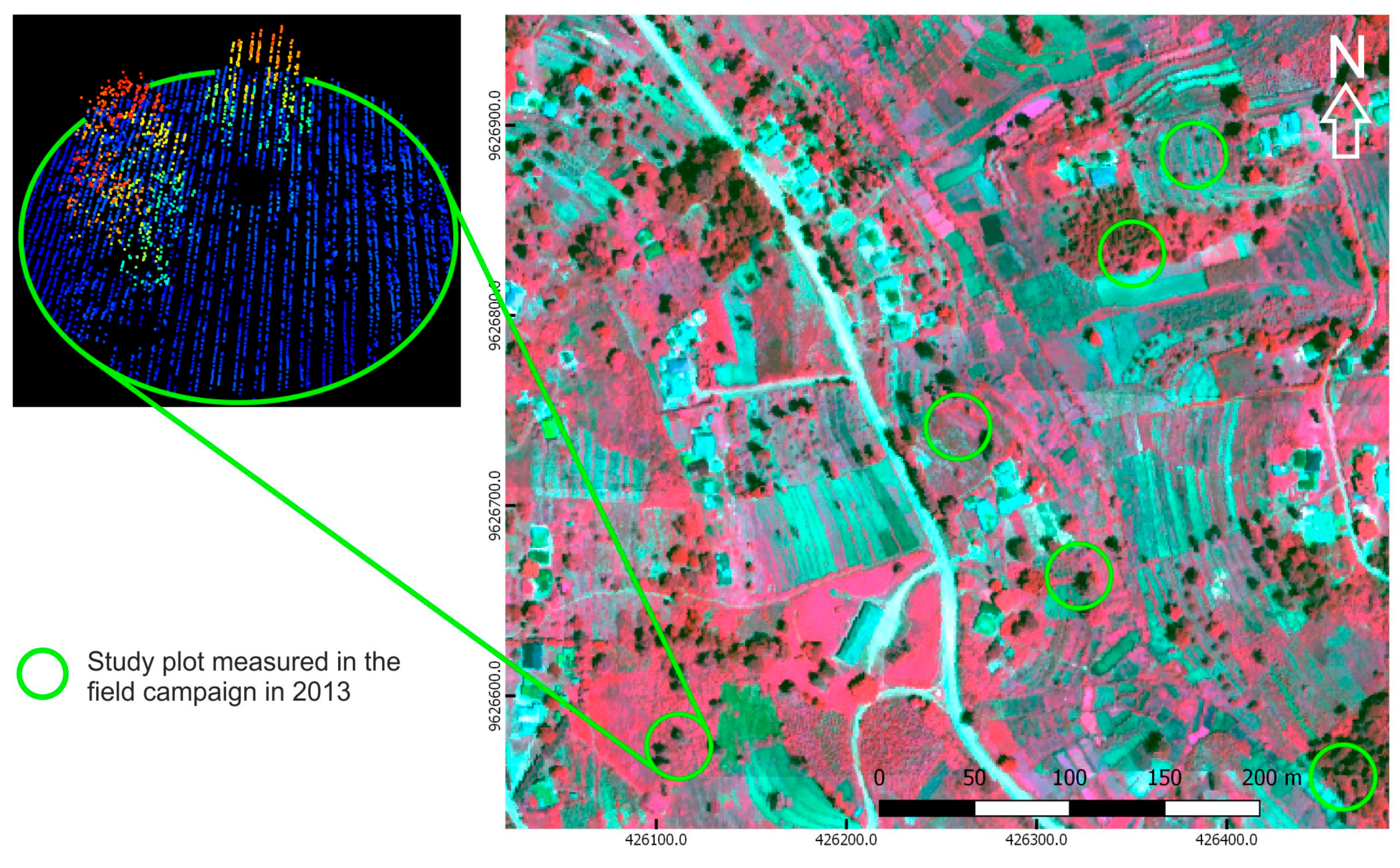
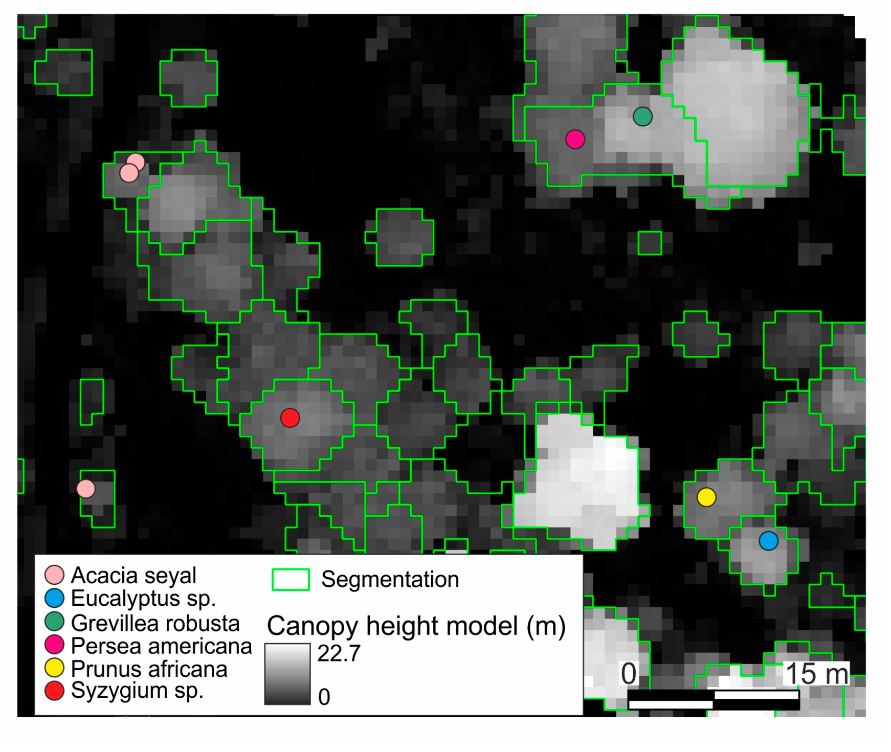
2.5. Segmentation and Preparing Training Data

Tree crowns were segmented using the dalponte2016 algorithm [36] implemented in the lidR package [37] in R software (R version 3.4.0, R Foundation for Statistical Computing) [38]. The algorithm finds local maxima from rasterized CHM, designates these as tree tops, and then uses a decision tree method to grow individual crowns around the local maxima.
We matched the 950 field measured trees to 543 tree crowns (Figure 4). If multiple field measurements from the same species were detected for the same segmented crown, only one of the observations would be kept. Thus, one segmented tree crown may consist of multiple trees from the same species, while one segment was considered as one sample. If a crown contained more than one species, it would be excluded. In total 61 species were observed for 543 crowns, while 19 of the species had only 1 observation and 10 had 2–3 observations. These were excluded from the classification as done in a similar setting earlier [10]. The classifications included in total 499 crowns from 31 species (Table 1). All species belonging to Eucalyptus and Syzygium genuses were labeled as Eucalyptus spp. and Syzygium spp., respectively, as we could not identify the exact species in all instances. However, the majority of the Eucalyptuses were Eucalyptus saligna.

2.6. Minimum Noise Fraction Transformation

MNF transformation [20] was applied to the atmospherically corrected reflectance data to reduce dimensionality and pack coherent information in a smaller set of features. The algorithm was applied in ENVI software (version 5.0, Research Systems Inc., Boulder, CO, USA) [39]. We determined the usefulness of the MNF components by the evaluation of their eigenvalues and through visual interpretation [40]. We selected 15 first MNF components and disregarded the rest based on their low eigenvalues. The further visual inspection confirmed that the MNF bands from 16 onwards contained mostly noise. Each MNF component has corresponding eigenvectors that can be used to interpret the weight that each original reflectance band has on the component.

2.7. Narrowband Vegetation Indices

We calculated a set of narrowband vegetation indices (NVI) that have been linked in earlier studies with vegetation structure, biochemistry and plant physiology (Table S1) [41]. Some of the indices have originally been developed for broadband data but were calculated using narrowband IS data and thus referred as NVIs.

2.8. Point cloud Features

We used lidR package [37] in R to calculate features for tree crown segments from the ALS point cloud. The average density was 9.6 pulses m2, but there was notable variation in pulse density due to elevation variations across the study area (Figure 1). Especially in the valleys, there were not enough returns per tree crown to calculate complex features. Intensity values were not considered as they were uncalibrated and IS data were available. As ALS derived height information alone is of limited value [9], we calculated variance (var), minimum height (min), 95th percentile (P95), median absolute deviation around median (MADmedian) , median absolute deviation around mean (MADmean), average absolute deviation around median (AADmedian), average absolute deviation around mean (AADmean), quadratic mean (QM), the count of returns (count), maximum height divided by the maximum crown diameter (HD) and maximum height divided by the count of returns (HC).

2.9. Feature Selection

We used VSURF (Variable Selection Using Random Forests) package in R [42,43] to perform the feature selection. VSURF uses the RF variable importance to identify the features that are the most important for the classification task. It was developed especially for handling high dimensional data. VSURF performs three steps: (1) irrelevant features are eliminated; (2) all features related to the response are selected (interpretation step); and (3) selection is refined by eliminating redundancy in the set of features selected in the second step (prediction step). The features retained in the final step were used to test the impact of variable selection on the classification accuracy and to identify the features that were important for the classification.

2.10. Classification Methods

All classifications were realized using “caret” package in R [44]. Specifically, we used “Kernlab” and “RandomForest” packages for SVM and RF, respectively [45,46]. We used the radial basis kernel with SVM and optimized C and sigma values through grid search. For RF, we set ntree to 500 and searched mtry value by testing values 4, 8, 16 and 32. As our dataset was imbalanced, we selected the models that produced the highest Kappa instead of overall accuracy (OA) [44].
The class balancing was done for the training data during the cross validation using the up-sampling method from “caret” package, while test data were left intact. The up-sampling method randomly samples (with replacement) the minority classes to be the same size as the majority class (class with most samples). Classifications using up-sampling are referred to as balanced classification from here on after.

2.11. Measures of Performance

OA was calculated as the total number of correctly classified samples divided by the total number of samples. We used precision and recall, equivalent to user’s and producer’s accuracy [47], to evaluate the performance on the class level. We calculated also F1-score, which is harmonic mean of precision and recall as following:
F 1 = 2 × ( p r e c i s i o n   × r e c a l l p r e c i s i o n + r e c a l l )
F1-score increases with higher precision or recall and with the higher similarity between the two values. The values range between 0 and 1, while the best value is 1 and worst is 0.

2.12. Jeffries–Matusita Distance

As we expected that some of the species cannot be classified individually and grouping all the species under an arbitrarily defined limit for minimum number of samples might not be meaningful, we used JM distance to find spectrally and structurally similar subgroups of species. The multiclass JM distances were calculated using the varSel package in R [48] using the best performing feature set. First, the JM distances were calculated for all species pairs. Next, the species with the least number of samples were grouped with the species with the lowest matching JM distance. The process was repeated until each species belonged to one of the groups. Finally, the process was repeated to achieve a smaller number of groups. The process was started from the species with the fewest samples to achieve groups with enough samples for building a stable classification model.

2.13. Statistical Significance Tests

McNemar’s test without continuum correction was used for testing statistical significance [18,49,50]. It is an appropriate method when the sample size is small [51]. Specifically, McNemar’s test was used to assess: (1) whether there were significant differences in the OAs between the different feature sets; (2) whether there were significant differences in the OAs between SVM and RF classification results; and (3) whether the feature selection had a significant impact. McNemar’s tests were calculated from leave-one-out cross validation (LOOCV) results. The limitation of McNemar’s test is that it does not measure the variation resulting from the choice of training sets or internal randomness of the algorithm. As the RF results vary between iterations, we repeated the LOOCV for RF classifier 50 times and used the mode of the prediction results of each sample when McNemar’s test results were classified.

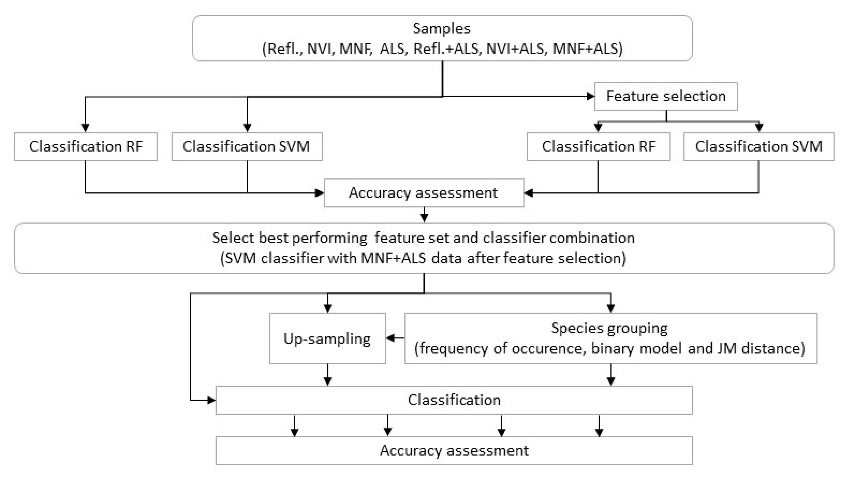
2.14. Classification Trials

All the classification trials are summarized in Figure 5. First, we classified all species with more than three samples using SVM and RF classifiers with the following feature sets: (1) reflectance; (2) NVI; (3) MNF; (4) ALS; (5) reflectance+ALS; (6) NVI+ALS; and (7) MNF + ALS features. Next, we run VSURF feature selection on all feature sets and repeated the classifications. Then, we evaluated the impact of feature selection on classification accuracy and identified important features. We selected the classifier and feature set that produced the highest Kappa values for later analysis of different approaches for grouping the species. In the final step, we tested different approaches for grouping species with fewer samples and tested the impact of up-sampling on the classification results.
The statistical significance between the different grouping approaches was not evaluated as the number of classes varied. Instead, we used 3-fold cross validation that was repeated 10 times to evaluate the stability of the classifier and interpreted the precision, recall and F1-scores. We tested three different approaches to group species. First, we grouped all species with less than 20 samples together to group “other” and classified the rest of the species separately as done earlier in a similar setting [10]. Next, we classified each of the species separately against a mixed group of all other species. The last approach was to use JM distance to combine species together, while species with high F1-scores and low variability were classified individually.

3. Results

3.1. Comparison of Feature Sets and Classifiers

The highest OA using both classifiers was achieved with MNF + ALS feature set (Table 2). There was a statistically significant difference (p < 0.05) between the SVM and RF classifications only when reflectance or NVI feature set was used (Table S2). MNF feature set outperformed reflectance, NVI and ALS feature sets with statistical significance. For SVM classification the fusion of ALS features with MNF features improved the OA with statistical significance, compared with the classification with only MNF features (Tables S3 and S4). For RF classification there was not statistically significant improvement between these feature sets. The highest classification accuracy was achieved with SVM classifier and MNF + ALS features set, but the improvement to RF classification with the same feature set was not statistically significant. Generally, the OAs were low, as many species with fewer samples performed poorly.

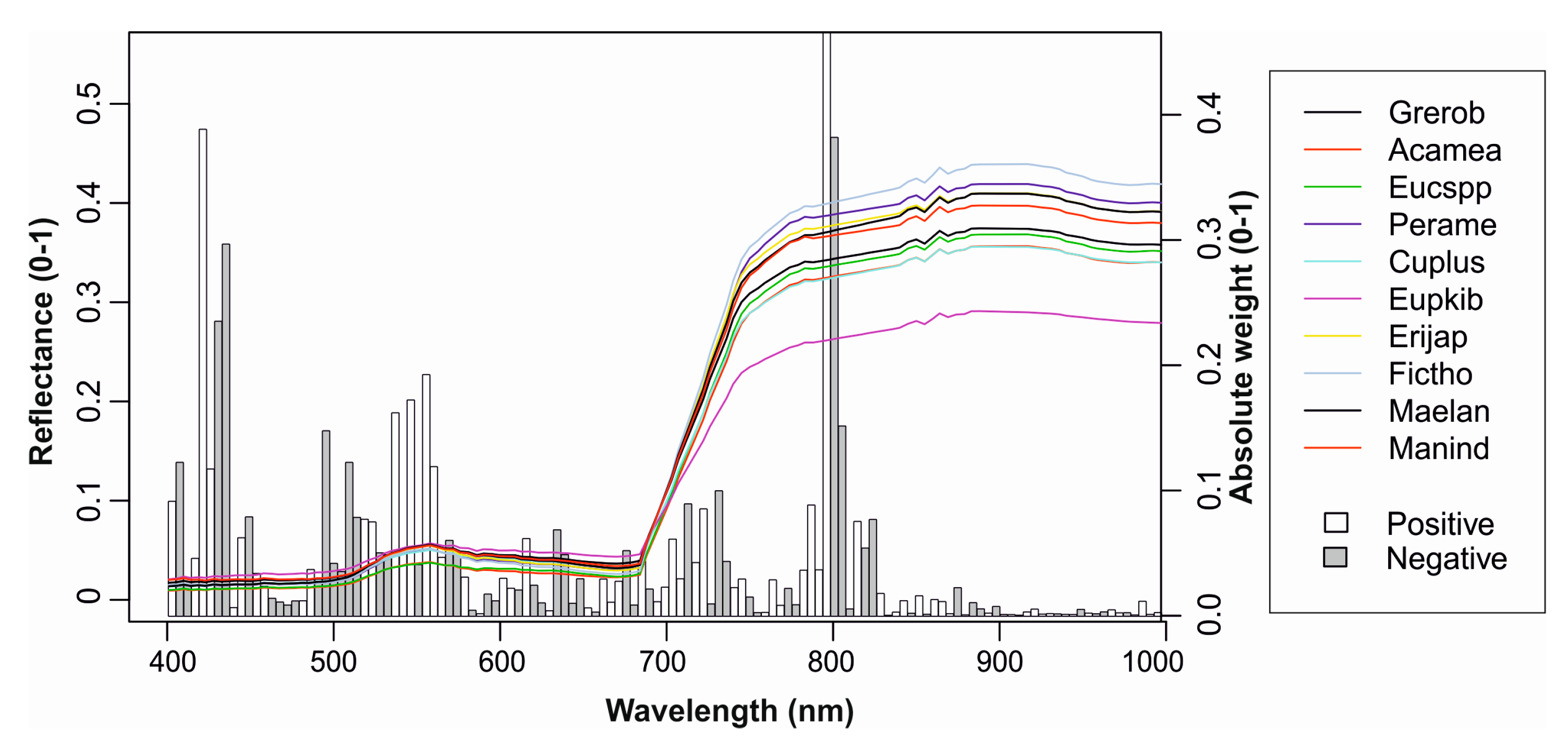
3.2. Feature Selection

Feature selection had only small impact on OA and Kappa (Table S5), while the change in OA was statistically significant only for the NVI feature set classified with the SVM classifier. However, we could achieve the same level of accuracy with a smaller number of input features (Table 3). The important spectral regions were found at 400–450 nm, while 550–570 and 700–800 nm were also important. The most important MNF component (MNF9) had high weights around the same areas where we found important spectral bands (Table 4 and Figure 6). Most important vegetation indices were anthocyanin content index (ACI) and anthocyanin reflectance index (ARI) (Table S1 and Table 4) that were calculated from spectral bands centered at 549, 698 and 788 nm that are also seen as spikes in the MNF9 component.

3.3. Jeffries–Matusita Distance
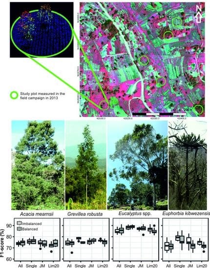
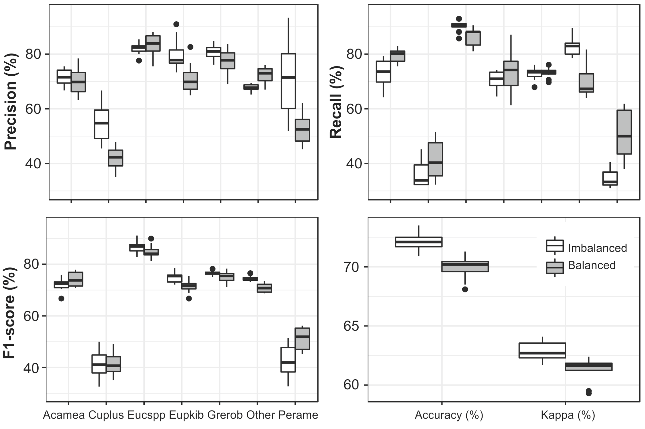
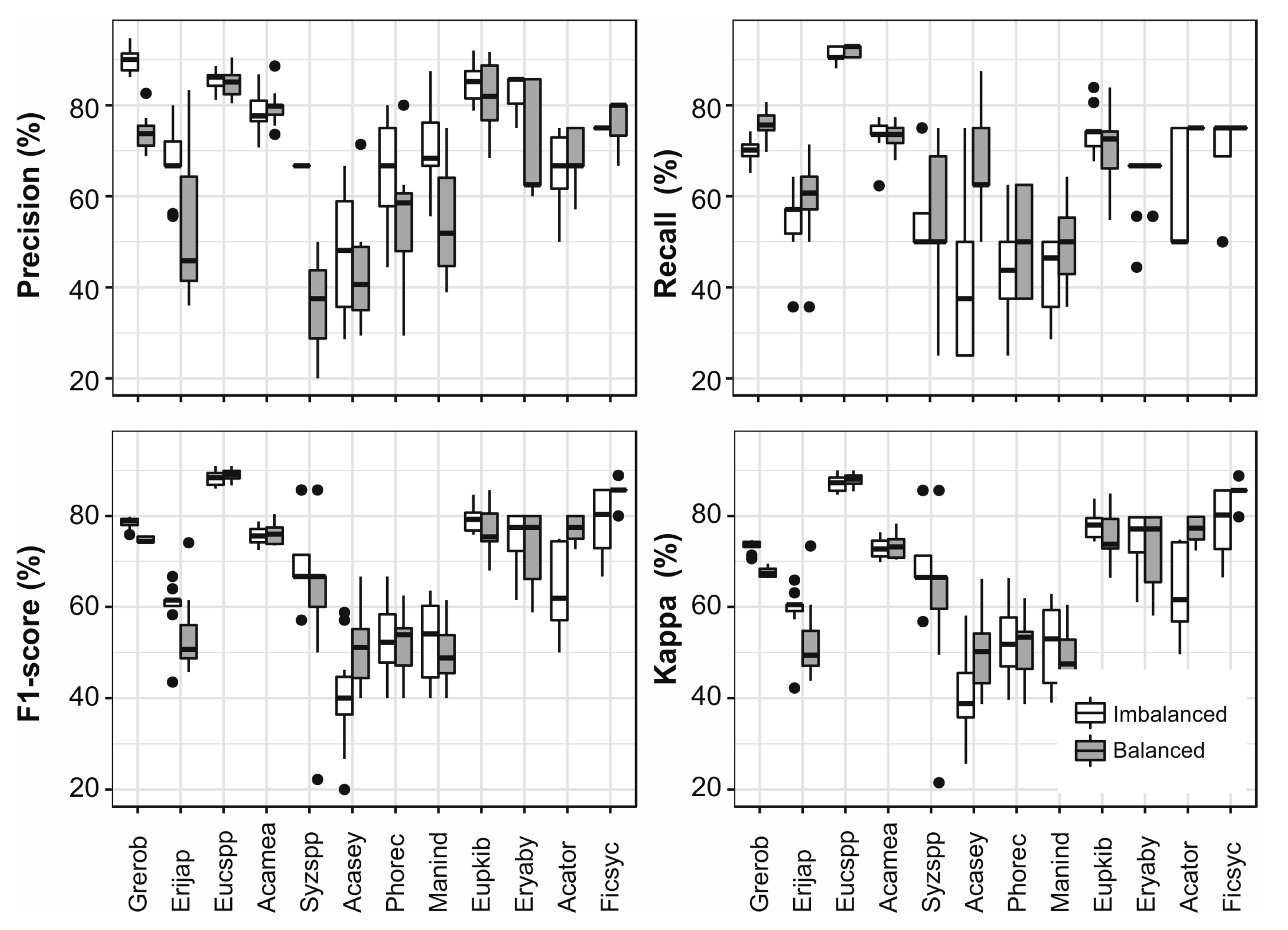
The spectral regions with the highest JM distances between species (nine species with most samples selected for closer inspection) were found most often near 400 nm and 550 nm (Figure 7). There were notable differences between species as, for example, Euphorbia kibwezensis did not have any bands with the highest distance between species around 470–740 nm, while we can see an important region around 750 nm, where the reflectance is notably lower in comparison with other species.

3.4. Data Balancing

The mean OA (10 iterations with the best performing feature set MNF + ALS with feature selection) was 57.1% for the imbalanced and 56.0% the balanced classification (all 31 species). The mean F1-scores ranged between 0% (Ficus sur) and 84.9% (Eucalyptus spp) in the imbalanced setting (Figure 8). Acacia mearnsii, Grevillea robusta, Eucalyptus spp. and Euphorbia kibwezensis had mean F1-scores of 73.8%, 74.6%, 84.9% and 71.7%, respectively, with low variability. The species with fewer samples had high variability and lower F1-scores. However, Erythrina abyssinica, Acacia tortilis and Ficus sycomorus with 9, 4 and 8 samples, respectively, performed better than Persea Americana and Cupressus lusitanica with 42 and 31 samples, respectively. Up-sampling had only minor impact on the results.

3.5. Grouping by Frequency

Combining the species with less than 20 samples increased the mean OA to 70.2% (imbalanced) and 69.2% (balanced), while mean Kappa was 62.9% and 61.3% for imbalanced and balanced classification, respectively (Figure 9). Up-sampling increased recall for Acacia mearnsii, Cupressus lucitanica and Persea Americana while precision decreased. We found a notable increase in the mean F1-score only for Persea americana while the F1-scores of species with more samples and higher initial classification accuracy decreased slightly.

3.6. Single Species Classfication

The up-sampling had the biggest impact on the results when the species were classified individually against all remaining species (Figure 10). The mean recall increased and mean precision decreased for most species. The mean F1-scores increased notably for Acacia seyal, Acacia tortilis and Ficus sycomorus from 40.2%, 64.3% and 82.6% to 51.3%, 77.3%, and 87.2%, respectively.

3.7. Grouping Species Based on Jeffries–Matusita Distance

The species with high F1-scores and low variability (Acacia mearnsii, Grevillea robusta, Eucalyptus spp. and Euphorbia kibwezensis) were classified separately, while four groups were created for the remaining species based on JM-distance (Table 4). Two of the groups were classified with F1-score > 60% while the other two had mean F1-scores around 50% (Figure 11). The mean OA was 66% and mean Kappa 61% while up-sampling had only a little impact on the overall performance. All species in Group 3 are fruit bearing trees with economic importance.

3.8. Comparison of Different Aproaches

We selected four of the species (Acacia mearnsii, Grevillea robusta, Eucalyptus spp. and Euphorbia kibwezensis) with the highest F1-scores for a closer comparison of how they were affected depending on how the remaining species were grouped (Figure 12). For the selected species, the highest mean precision and F1-scores were achieved when the species were classified individually against mixed groups of all other species. The highest recall for Acacia mearnsii and Grevillea robusta, the species with the greatest number of samples, was achieved when all 31 species were classified separately.

4. Discussion

4.1. Impacts of Classifier, Feature Selection and Data Fusion

Both SVM and RF classifiers have been reported performing well in remote sensing based classifications, while neither is constantly outperforming the other [17,18,19]. In our results, there was no statistically significant difference between the two classifiers with the best performing feature set (MNF + ALS). Previous research has shown that fusing ALS data with IS data may increase the classification accuracy, while canopy height information alone is often not enough for the improved results [9,18,52]. In our results, the impact of data fusion depended on the classifier and how the IS data were used. For example, SVM classifier benefited from data fusion when ALS data were combined with MNF data, while RF classifier did not. The most important ALS derived feature was the maximum height divided by the maximum crown diameter. This is logical as, for example, Eucalyptus spp. and Grevillea Robusta are very tall trees with narrow crowns, while acacias tend to have wider crowns in relation to their height. Our ALS feature set was limited because of discrete return ALS data while full waveform ALS data could yield even bigger improvements [53].
Feature selection did not have statistically significant impact on the best performing feature set MNF + ALS. However, it was still useful, given that the same accuracies were achieved with fewer features, making the training and execution of the models faster. In addition, we used feature selection to find the features that were important for the classification procedure. In a recent review, the near-infrared wavelength regions that were important for tree species classification were found most commonly at 450–550 nm and 650–700 nm [9]. In our results, the most important regions were found at 400–450 nm, 550–570 nm and 700–800 nm. The most common important spectral region in the summary was at 650 nm, which was not important in our study. In our results, the wavelengths near 400 nm were especially important, which was selected as important wavelength area in 38% of the studies in the review [9]. The wavelength regions between 800–1000 nm were not commonly important, which was the same in our study. We did not have SWIR data available, which has important wavelengths, for example, near 1200 nm and 1450 nm, which might increase the classification accuracy.

4.2. The Impact of Up-Sampling and Grouping of Species on the Classification Results

The OA and Kappa were low when all the 31 species were classified separately. However, when species with fewer than 20 samples were combined, we reached higher OA and Kappa than in a recent study conducted in a similar landscape in Panama [10]. However, our data had fewer species with more than 20 samples. In addition, the F1-scores ranged similarly with high variability between species.
The high F1-score (with low variability) for Eucalyptus spp. enables map production for conservation planning. However, it needs to be considered that species with less than four samples were removed from the model (8.1% field measurements with matching tree crown). The highest F1-score for Eucalyptus spp. was achieved when it was classified against a mixed group of all the other species using up-sampling. However, the difference between up-sampling and imbalanced model was marginal. In addition, Acacia mearnsii, Grevillea robusta and Euphorbia kibwezensis, could be mapped with relatively high accuracy. Acacia mearnsii is highly invasive and monitoring its distribution in the long term would be valuable for conservation planning. Euphorbia kibwezensis, a dry land species, could possibly be used to study linkages between changes in climate and the occurrence of the species, as done earlier with Euphorbia ingens in South Africa [54]. Species with fewer samples, Ficus sycomorus, Acacia tortilis, Erythrina abyssinica and Syzygium spp., were also classified with relatively high mean F1-scores in the single species setting. However, the small sample size and high variability in the results make it difficult to assess how the models would perform when extended over the whole study area. Cupressus lusitanica was classified with poor accuracy, possibly because it is used in fences where it grows densely and achieve low maximum heights, but it is also used in plantations for lumber production, where it reaches much higher heights. Persea americana was classified with poor accuracy, which could be explained by spectral and structural similarities with a number of other fruit trees. As hyperspectral data also capture the phenological states of trees [55], it is possible that some of the misclassifications can be explained by the spectral variation caused by different phenology resulting from the varying local climate caused by topography.
In the previous studies with a high number of species, a mixed group of species with fewer samples has been commonly used [10,56]. However, combining all the species under a fixed limit (e.g., 20 samples) creates large and highly heterogeneous mixed class. On the other hand, spectral similarity measures, like JM distance, can be used to find spectrally and structurally similar species, which enables creating smaller and more homogeneous groups that also balance the training data. For example, Group 3 created with this approach has two exotic (Persea Americana and Mangifera indica) and three native (Ficus sur, Syzygium spp. and Bridelia micrantha) fruit bearing tree species. The sixth species, Phoenix reclinata, is a palm that produces edible fruits (dates). Thus, it is also an ecologically meaningful group as all of the species are fruit bearing. Based on our results, JM distance may help in identifying groups of species that could be classified together with acceptable accuracy. However, grouping the species using JM distance makes sense only if the created groups have a common ecological or economic function. Up-sampling did not improve OA or Kappa, but we did see improvements on the species level, usually for species with smaller sample sizes or lower initial classification accuracy.

4.3. Evaluation of the Quality of Airborne Data, Field Measurements and Segmentation

As the airborne data were acquired in 2013 and the later field campaign was conducted in 2015, it was difficult to estimate if a tree had been over five meters tall two years ago. Thus, some of the trees measured in 2015 might have been left undetected by the segmentation algorithm. In addition, some of the species (e.g., Acacia mearnsii) grow in dense bush-like formations, which were problematic for the segmentation algorithm, as the crowns were difficult to separate even in the visual interpretation of the CHM. For example, one of the segmented tree crowns contained six Acacia mearnsii field measurements. Generally, isolated trees on farmland were easier for the segmentation algorithm, but naturally growing trees with tightly knit canopy structure were challenging, which underlies the difficulty of accurate tree crown segmentation in the tropical areas with dense canopies [11,57]. Furthermore, the positional accuracy was low in some areas due to the mountainous nature of the study area and only one available GNSS base station. Removing all field measurements with positional accuracy lower than four meters helped, but still some of the field measurements might have been matched with wrong tree crown.

5. Conclusions

Our results demonstrate that, even in diverse African agroforestry landscapes with high species diversity and imbalanced training data, the classification of some species, or groups of species, is possible when proper pre-processing, feature transformation and species grouping approaches are used. The MNF transformed data combined with the ALS features was superior in performance when compared with the other feature sets, and the best results were achieved with SVM classifier. If the aim is only to map the distribution of one species at the time, we suggest combining all the other species into one mixed group, as the highest accuracies were achieved with this approach. If many species are classified at the same time, the spectral separability measures like JM distance can be used to find spectrally and structurally similar groups of species. With this approach, we found an ecologically and economically meaningful group of six fruit bearing trees that can be mapped with moderate accuracy. The up-sampling improved the F1-scores for some species with fewer samples. For example, Acacia tortilis with only four samples was classified with high mean F1-score after up-sampling. However, due to the small sample size, it is difficult to assess the performance of the model when predicted over the whole study area. Our results also provide important insights into the spectral and structural features that differentiate the tree species in the study area, while we found notable differences in the important spectral regions compared with previous studies. The three non-native tree species (Eucalyptus spp., Grevillea robusta, and Acacia mearnsii) that could be mapped with the highest accuracies account for 40.1% of the samples. Thus, it is possible to map the decrease in biodiversity indirectly by mapping changes in the distribution of these species, as the increase in their distribution could mean decrease in the number of native tree species. In addition, Eucalyptus spp. and Acacia mearnsii are highly invasive species, and mapping their distribution would be valuable for conservation planning. Grevillea robusta is an important agroforestry tree and mapping their distribution would provide valuable information for the characterization of agroforestry practices in the study area. Although the number of species that were classified accurately is relatively low, better results could be achieved with more representative field data.

Supplementary Materials

The following are available online at www.mdpi.com/2072-4292/9/9/875/s1, Table S1: List of narrowband vegetation indices, Table S2: McNemar’s score and statistical significance of difference in overall accuracy between support vector machine and random forest classifiers for different feature sets, Table S3: McNemar’s score (lower triangular part) and statistical significance of difference in overall accuracy (upper triangular part) between different feature sets using support vector machine; Table S4: McNemar’s score (lower triangular part) and statistical significance of change in overall accuracy (upper triangular part) between different feature sets using random forest, Table S5: Change in overall accuracy and Kappa after feature selection.

Acknowledgments

This research was funded by Ministry for Foreign Affairs of Finland (CHIESA and BIODEV projects) and Academy of Finland (TAITAWATER project). The authors want to thank Jessica Broas and Kirsi Kivistö from University of Helsinki and Darius Kimuzi from Taita Research Station for helping to collect the field data in 2013 and 2015. Jesse Hietanen preprocessed the ALS point clouds. Elisa Schäfer, Kirsi Kivistö and Hari Adhikari helped to orthorectify the AisaEAGLE data. Pekka Hurskainen and Fabian Fassnacht offered valuable comments on the manuscript. Taita Research Station of the University of Helsinki in Kenya and its staff are warmly acknowledged for logistical support and safe accommodation during the fieldwork. Research permit NCST/RCD/17/012/33 from National Council for Science and Technology of Republic of Kenya is warmly acknowledged.

Author Contributions

R.P., J.H., E.M. and P.P. conceived and designed the experiments. R.P. performed the experiments and analyzed the data. J.H., E.M. and A.V. contributed materials and analysis tools. R.P. wrote the paper.

Conflicts of Interest

The authors declare no conflict of interest.

References

  1. Gibbs, H.K.; Ruesch, A.S.; Achard, F.; Clayton, M.K.; Holmgren, P.; Ramankutty, N.; Foley, J.A. Tropical forests were the primary sources of new agricultural land in the 1980s and 1990s. Proc. Natl. Acad. Sci. USA 2010, 107, 16732–16737. [Google Scholar] [CrossRef] [PubMed]
  2. Brink, A.B.; Bodart, C.; Brodsky, L.; Defourney, P.; Ernst, C.; Donney, F.; Lupi, A.; Tuckova, K. Anthropogenic pressure in East Africa—Monitoring 20 years of land cover changes by means of medium resolution satellite data. Int. J. Appl. Earth Obs. Geoinf. 2014, 28, 60–69. [Google Scholar] [CrossRef]
  3. Mbow, C.; van Noordwijk, M.; Prabhu, R.; Simons, T. Knowledge gaps and research needs concerning agroforestry’s contribution to Sustainable Development Goals in Africa. Curr. Opin. Environ. Sustain. 2014, 6, 162–170. [Google Scholar] [CrossRef]
  4. Luedeling, E.; Kindt, R.; Huth, N.I.; Koenig, K. Agroforestry systems in a changing climate—Challenges in projecting future performance. Curr. Opin. Environ. Sustain. 2014, 6, 1–7. [Google Scholar] [CrossRef]
  5. Rodriguez-Suarez, J.A.; Soto, B.; Perez, R.; Diaz-Fierros, F. Influence of Eucalyptus globulus plantation growth on water table levels and low flows in a small catchment. J. Hydrol. 2011, 396, 321–326. [Google Scholar] [CrossRef]
  6. Lott, J.E.; Khan, A.A.H.; Black, C.R.; Ong, C.K. Water use in a Grevillea robusta-maize overstorey agroforestry system in semi-arid Kenya. For. Ecol. Manag. 2003, 180, 45–59. [Google Scholar] [CrossRef]
  7. Omoro, L.M.A.; Nair, P.K.R. Effects of mulching with multipurpose-tree prunings on soil and water run-off under semi-arid conditions in Kenya. Agrofor. Syst. 1993, 22, 225–239. [Google Scholar] [CrossRef]
  8. Thijs, K.W.; Aerts, R.; van de Moortele, P.; Aben, J.; Musila, W.; Pellikka, P.; Gulinck, H.; Muys, B. Trees in a human-modified tropical landscape: Species and trait composition and potential ecosystem services. Landsc. Urban Plan. 2015, 144, 49–58. [Google Scholar] [CrossRef]
  9. Fassnacht, F.E.; Latifi, H.; Sterenczak, K.; Modzelewska, A.; Lefsky, M.; Waser, L.T.; Straub, C.; Ghosh, A. Review of studies on tree species classification from remotely sensed data. Remote Sens. Environ. 2016, 186, 64–87. [Google Scholar] [CrossRef]
  10. Graves, S.J.; Asner, G.P.; Martin, R.E.; Anderson, C.B.; Colgan, M.S.; Kalantari, L.; Bohlman, S.A. Tree species abundance predictions in a tropical agricultural landscape with a supervised classification model and imbalanced data. Remote Sens. 2016, 8, 161. [Google Scholar] [CrossRef]
  11. Feret, J.-B.; Asner, P.G. Tree species discrimination in tropical forests using airborne imaging spectroscopy. IEEE Trans. Geosci. Remote Sens. 2013, 51, 73–84. [Google Scholar] [CrossRef]
  12. Baldeck, C.A.; Asner, G.P. Improving remote species identification through efficient training data collection. Remote Sens. 2014, 6, 2682–2698. [Google Scholar] [CrossRef]
  13. Freeman, E.A.; Moisen, G.G.; Frescino, T.S. Evaluating effectiveness of down-sampling for stratified designs and unbalanced prevalence in Random Forest models of tree species distributions in Nevada. Ecol. Model. 2012, 233, 1–10. [Google Scholar] [CrossRef]
  14. Dalponte, M.; Ene, L.T.; Marconcini, M.; Gobakken, T.; Næsset, E. Semi-supervised SVM for individual tree crown species classification. ISPRS J. Photogramm. Remote Sens. 2015, 110, 77–87. [Google Scholar] [CrossRef]
  15. Vapnik, V. Statistical Learning Theory; John Wiley & Sons: New York, NY, USA, 1998. [Google Scholar]
  16. Breiman, L.E.O. Random Forests. Mach. Learn. 2001, 45, 5–32. [Google Scholar] [CrossRef]
  17. Belgiu, M.; Drăguţ, L. Random forest in remote sensing: A review of applications and future directions. ISPRS J. Photogramm. Remote Sens. 2016, 114, 24–31. [Google Scholar] [CrossRef]
  18. Ghosh, A.; Fassnacht, F.E.; Joshi, P.K.; Kochb, B. A framework for mapping tree species combining hyperspectral and LiDAR data: Role of selected classifiers and sensor across three spatial scales. Int. J. Appl. Earth Obs. Geoinf. 2014, 26, 49–63. [Google Scholar] [CrossRef]
  19. Ghosh, A.; Joshi, P.K. A comparison of selected classification algorithms for mappingbamboo patches in lower Gangetic plains using very high resolution WorldView 2 imagery. Int. J. Appl. Earth Obs. Geoinf. 2014, 26, 298–311. [Google Scholar] [CrossRef]
  20. Green, A.; Berman, M.; Switzer, P.; Craig, M.D. A transformation for ordering multispectral data in terms of image quality with implications for noise removal. IEEE Trans. Geosci. Remote Sens. 1988, 26, 65–74. [Google Scholar] [CrossRef]
  21. Piiroinen, R.; Heiskanen, J.; Mõttus, M.; Pellikka, P. Classification of crops across heterogeneous agricultural landscape in Kenya using AisaEAGLE imaging spectroscopy data. Int. J. Appl. Earth Obs. Geoinf. 2015, 39. [Google Scholar] [CrossRef]
  22. Jaetzold, R.; Schmidt, H.; Hornetz, B.; Shisanya, C. Farm Management Handbook of Kenya: Natural Conditions and Farm Management Information; Ministry of Agriculture, Kenya & German Agricultural Team; German Agency for Technical Cooperation: Rossdorf, Germany, 1983; Volume 2. [Google Scholar]
  23. Aerts, R.; Thijs, K.W.; Lehouck, V.; Beentje, H.; Bytebier, B.; Matthysen, E.; Gulinck, H.; Lens, L.; Muys, B. Woody plant communities of isolated Afromontane cloud forests in Taita Hills, Kenya. Plant Ecol. 2011, 212, 639–649. [Google Scholar] [CrossRef] [Green Version]
  24. Clark, B.; Pellikka, P. Landscape analysis using multi-scale segmentation and objectoriented classification. Recent Adv. Remote Sens. 2009, 323–341. [Google Scholar]
  25. Pellikka, P.K.E.; Clark, B.J.F.; Gosa, A.G.; Himberg, N.; Hurskainen, P.; Maeda, E.; Mwang’ombe, J.; Omoro, L.M.A.; Siljander, M. Agricultural expansion and its consequences in the Taita Hills, Kenya. Dev. Earth Surf. Process. 2013, 16, 165–179. [Google Scholar] [CrossRef]
  26. Burgess, N.D.; Butynski, T.M.; Cordeiro, N.J.; Doggart, N.H.; Fjeldså, J.; Howell, K.M.; Kilahama, F.B.; Loader, S.P.; Lovett, J.C.; Mbilinyi, B.; et al. The biological importance of the Eastern Arc Mountains of Tanzania and Kenya. Biol. Conserv. 2007, 134, 209–231. [Google Scholar] [CrossRef]
  27. Pellikka, P.K.E.; Lötjönen, M.; Siljander, M.; Lens, L. Airborne remote sensing of spatiotemporal change (1955–2004) in indigenous and exotic forest cover in the Taita Hills, Kenya. Int. J. Appl. Earth Obs. Geoinf. 2009, 11, 221–232. [Google Scholar] [CrossRef]
  28. Hohenthal, J.; Räsänen, M.; Owidi, E.; Andersson, B.; Minoia, P.; Pellikka, P.K.E. Community and Institutional Perspectives on Water Management and Environmental Changes in the Taita Hills, Kenya; University of Helsinki: Helsinki, Finland, 2015; ISBN 9789515113412. [Google Scholar]
  29. Mugedo, J.Z.A.; Waterman, P.G. Sources of tannin: Alternatives to wattle (Acacia mearnsii) among indigenous Kenyan species. Econ. Bot. 1992, 46, 55–63. [Google Scholar] [CrossRef]
  30. Boudiaf, I.; Le Roux, C.; Baudoin, E.; Galiana, A.; Beddiar, A.; Prin, Y.; Duponnois, R. Soil Bradyrhizobium population response to invasion of a natural Quercus suber forest by the introduced nitrogen-fixing tree Acacia mearnsii in El Kala National Park, Algeria. Soil Biol. Biochem. 2014, 70, 162–165. [Google Scholar] [CrossRef]
  31. Engeman, R.M.; Sugihara, R.T.; Pank, L.F.; Dusenberry, W.E. A comparison of plotless density estimators using Monte Carlo simulation. Ecology 1994, 75, 1769–1779. [Google Scholar] [CrossRef]
  32. Khosravipour, A.; Skidmore, A.K.; Isenburg, M.; Wang, T.; Hussin, Y. Generating pit-free canopy height models from airborne lidar. Photogramm. Eng. Remote Sens. 2014, 80, 863–872. [Google Scholar] [CrossRef]
  33. Richter, R.; Schläpfer, D. Geo-atmospheric processing of airborne imaging spectrometry data. Part 2: Atmospheric/topographic correction. Int. J. Remote Sens. 2002, 23, 2631–2649. [Google Scholar] [CrossRef]
  34. Valbuena, R. Integrating airborne laser scanning with data from global navigation satellite systems and optical sensors. In Forestry Applications of Airborne Laser Scanning: Concepts and Case Studies; Maltamo, M., Naesset, E., Vauhkonen, J., Eds.; Springer: Berlin, Germany, 2014; Volume 27, pp. 63–88. [Google Scholar]
  35. Baldeck, C.A.; Asner, G.P.; Martin, R.E.; Anderson, C.B.; Knapp, E.; Kellner, J.R.; Wright, S.J. Operational tree species mapping in a diverse tropical forest with airborne imaging spectroscopy. PLoS ONE 2015. [Google Scholar] [CrossRef] [PubMed]
  36. Dalponte, M.; Coomes, D.A. Tree-centric mapping of forest carbon density from airborne laser scanning and hyperspectral data. Methods Ecol. Evol. 2016, 7, 1236–1245. [Google Scholar] [CrossRef] [PubMed]
  37. Roussel, J.-R.; Auty, D. lidR: Airborne LiDAR Data Manipulation and Visualization for Forestry Applications, Version 1.2.0. Available online: https://rdrr.io/cran/lidR/ (accessed on 13 June 2017).
  38. R Core Team. R: A Language and Environment for Statistical Computing; Version 3.4.0; R Foundation for Statistical Computing: Vienna, Austria, 2017. [Google Scholar]
  39. RSI. ENVI User’s Guide; Research Systems, Inc.: Boulder, CO, USA, 2004; pp. 1–1150. [Google Scholar]
  40. Zhang, C.; Xie, Z. Combining object-based texture measures with a neural network for vegetation mapping in the Everglades from hyperspectral imagery. Remote Sens. Environ. 2012, 124, 310–320. [Google Scholar] [CrossRef]
  41. Roberts, D.A.; Roth, K.L.; Perroy, R.L. Hyperspectral vegetation indices. In Hyperspectral Remote Sensing of Vegetation; Thenkabail, P.S., Lyon, P.S., Huete, J.G., Eds.; CRC press: Boca Raton, FL, USA, 2011; pp. 309–328. [Google Scholar]
  42. Genuer, R.; Poggi, J.-M.; Tuleau-Malot, C. Variable selection using random forests. Pattern Recognit. Lett. 2010, 31, 2225–2236. [Google Scholar] [CrossRef]
  43. Genuer, R.; Poggi, J.-M.; Tuleau-Malot, C. VSURF: An R package for variable selection using random forests. R J. 2015, 7, 19–33. [Google Scholar]
  44. Kuhn, M. Building Predictive Models in R Using the caret Package. J. Stat. Softw. 2008, 28, 1–26. [Google Scholar] [CrossRef]
  45. Karatzoglou, A.; Smola, A.; Hornik, K.; Zeileis, A. kernlab—An S4 Package for Kernel Methods in R. J. Stat. Softw. 2004, 11, 1–20. [Google Scholar] [CrossRef]
  46. Liaw, A.; Wiener, M. Classification and Regression by randomForest. R News 2002, 2, 18–22. [Google Scholar] [CrossRef]
  47. Congalton, R.G. A review of assessing the accuracy of classifications of remotely sensed data. Remote Sens. Environ. 1991, 37, 35–46. [Google Scholar] [CrossRef]
  48. Dalponte, M.; Ørka, H.O. varSel: Sequential Forward Floating Selection Using Jeffries-Matusita Distance. Available online: https://rdrr.io/cran/varSel/ (accessed on 5 November 2016).
  49. Ballanti, L.; Blesius, L.; Hines, E.; Kruse, B. Tree species classification using hyperspectral imagery: A comparison of two classifiers. Remote Sens. 2016, 8, 445. [Google Scholar] [CrossRef]
  50. Foody, G.M. Thematic map comparison: evaluating the statistical significance of differences in classification accuracy. Photogramm. Eng. Remote Sens. 2004, 70, 627–633. [Google Scholar] [CrossRef]
  51. Dietterich, T.G. Approximate statistical tests for comparing supervised classi cation learning algorithms. Neural Comput. 1998, 10, 1895–1923. [Google Scholar] [CrossRef] [PubMed]
  52. Jones, T.G.; Coops, N.C.; Sharma, T. Assessing the utility of airborne hyperspectral and LiDAR data for species distribution mapping in the coastal Pacific Northwest, Canada. Remote Sens. Environ. 2010, 114, 2841–2852. [Google Scholar] [CrossRef]
  53. Hovi, A.; Korhonen, L.; Vauhkonen, J.; Korpela, I. LiDAR waveform features for tree species classification and their sensitivity to tree- and acquisition related parameters. Remote Sens. Environ. 2016, 173, 224–237. [Google Scholar] [CrossRef]
  54. Van Der Linde, J.A.; Roux, J.; Wingfield, M.J.; Six, D.L. Die-off of giant Euphorbia trees in South Africa: Symptoms and relationships to climate. S. Afr. J. Bot. 2012, 83, 172–185. [Google Scholar] [CrossRef]
  55. Landmann, T.; Piiroinen, R.; Makori, D.M.; Abdel-Rahman, E.M.; Makau, S.; Pellikka, P.; Raina, S.K. Application of hyperspectral remote sensing for flower mapping in African savannas. Remote Sens. Environ. 2015, 166, 50–60. [Google Scholar] [CrossRef]
  56. Colgan, M.S.; Baldeck, C.A.; Féret, J.-B.; Asner, G.P. Mapping savanna tree species at ecosystem scales using support vector machine classification and BRDF correction on airborne hyperspectral and LiDAR data. Remote Sens. 2012, 4, 3462–3480. [Google Scholar] [CrossRef]
  57. Clark, M.L.; Roberts, D.A. Species-Level Differences in Hyperspectral Metrics among Tropical Rainforest Trees as Determined by a Tree-Based. Remote Sens. 2012, 4, 1820–1855. [Google Scholar] [CrossRef]
Figure 1. Location of the study area in Coast Province of Kenya and trees sampled in 2013 and 2015.
Remotesensing 09 00875 g001
Figure 2. (a) Aerial view of town of Wundanyi and surrounding agroforestry landscape with forest fragments; (b) agroforestry landscape near Ngangao forest; and (c) Grevillea robusta; (d) Eucalyptus saligna; (e) Acacia mearnsii; (f) Persea americana; and (g) Euphorbia kibwezensis trees in a valley in the north-western corner of the study area.
Remotesensing 09 00875 g002
Figure 3. An example of AisaEAGLE data (color-infrared) and point cloud derived from laser scanning data. The coordinates are in UTM37S/WGS84 coordinate system.
Remotesensing 09 00875 g003
Figure 4. An example of segmented tree crowns and the field measured trees on top of the canopy height model.
Remotesensing 09 00875 g004
Figure 5. Workflow for the classification trials.
Remotesensing 09 00875 g005
Figure 6. Contribution (weight) of different wavelengths on the most important MNF component (MNF9; vertical bars) plotted over mean spectra of 10 species with most samples. Bars represent the absolute weight and sign is indicated with color (positive, negative).
Remotesensing 09 00875 g006
Figure 7. Reflectance (mean and standard deviation) for selected species and the wavelengths with the greatest JM distances between species (vertical lines).
Remotesensing 09 00875 g007
Figure 8. F1-scores for all species (more than three samples) in imbalanced and balanced (up-sampling) setting using support vector machine classifier and features selected by VSURF (MNF + ALS).
Remotesensing 09 00875 g008
Figure 9. Precision, Recall and F1-scores for the species with more than 20 samples and Other class in balanced and imbalanced setting using support vector machine classifier and features selected by VSURF (MNF + ALS).
Remotesensing 09 00875 g009
Figure 10. Classification results when each species was classified individually against mixed group of all other species (results shown for species with F1-score > 50%) in balanced and imbalanced setting (SVM classifier and MNF + ALS feature set with feature selection). The class level accuracies for the “other” class are not shown.
Remotesensing 09 00875 g010
Figure 11. Classification results with JM distance based class grouping in balanced and imbalanced setting using support vector machine classifier and features selected by VSURF (MNF + ALS).
Remotesensing 09 00875 g011
Figure 12. Comparison of precision, recall and F1-score for the selected tree species with different grouping methods and up-sampling (All = all 31 species classified individually, Single = each species is classified against mixed group of all other species, JM = JM distance used to group species, Lim20 = species with fewer than 20 samples grouped together).
Remotesensing 09 00875 g012
Table 1. Species with more than three samples, abbreviation used in figures, type (exotic or native), the frequency of the species (crown level) and number of pixels per species.
SpeciesAbbreviationTypeCrownsPixels
Grevillea robustaGrerobexotic1095485
Acacia mearnsiiAcameaexotic532437
Eucalyptus spp.Eucsppexotic422577
Persea americanaPerameexotic421989
Cupressus lusitanicaCuplusexotic311641
Euphorbia kibwezensisEupkibnative311181
Eriobotrya japonicaErijapexotic14516
Ficus thonningiiFicthonative14948
Maesa lanceolataMaelannative14612
Mangifera indicaManindexotic14668
Zimmermania ovataZimovanative13674
Zimmermania commiphoraZimcomnative11426
Psidium guajavaPsiguaexotic10459
Erythrina abyssinicaEryabynative9415
Acacia seyalAcaseynative8417
Phoenix reclinataPhorecnative8442
Albizia gummiferaAlbgumnative7387
Prunus africanaPruafrnative7410
Bridelia micranthaBrimicnative6335
Dombeya kirkiiDomkirnative6138
Ficus surFicsurnative6311
Combretum collinumComcolnative5234
Cussonia spicataCusspinative5215
Macademia spp.Macsppexotic5122
Millettia oblataMiloblnative5401
Acacia tortilisAcatornative490
Dombeya rotundifoliaDomrotnative4169
Ficus sycomorusFicsycnative4228
Newtonia buchananiiNewbucnative4385
Syzygium spp.Syzsppnative4174
Xymalos monosporaXymmonnative4123
Table 2. Classification results for the different feature sets using support vector machine and random forest classifiers with all of the species with more than three samples classified separately.
Support Vector Machine Random Forest
Feature SetAccuracyKappa AccuracyKappa
Refl.37.930.9 31.721.6
NVI45.537.5 35.925.8
MNF53.346.8 51.344.8
ALS31.721.6 30.721.8
Refl.+ALS42.935.7 42.935.6
NVI+ALS43.537.2 44.337.5
MNF + ALS57.152.1 54.148.2
Table 3. Features selected by VSURF at prediction phase for the different feature sets. The features are ordered based on their importance starting from the most important.
Feature SetNo Var.Feature Names
Refl.19R406, R401, R553, R549, R414, R562, R419, R572, R769, R717, R576, R530, R526, R521, R581, R458, R688, R632, R674
NVI8ACI, ARI, CIred edge, PRI, PSSR, mCARI, CRI1, EVI
MNF10MNF9, MNF1, MNF5, MNF7, MNF6, MNF4, MNF8, MNF10, MNF14, MNF2
ALS5HD, MADmedian, P95, AADmedian, min
Refl. + ALS15HD, max, MADmedian, MADmean, AADmedian, R406, R562, R558, min, R414, R423, R726, R731, R540, R774
NVI + ALS17ACI, HD, ARI, P95, max, MADmedian, CARI, AADmedian, AADmean, CRI2, CIred edge, HC, min, PRI, PSSR, SR, VIgreen
MNF + ALS13MNF9, HD, MNF5, MNF1, MNF4, MNF8, MNF7, MNF6, MNF11, MNF12, P95, MNF10, MNF14
R = reflectance, MNF = minimum noise fraction
Table 4. Groups generated using JM distances and the total number of samples in each group.
GroupSpecies in the GroupSamples
1Macspp, Maelan, Erijap, Domrot, Xymmon, ComCol, Zimova 59
2Zimcom, Eryaby, Acasey, Acator, Domkir 38
3Perame, Ficsur, Phorec, Manind, Brimic, Syzspp80
4Psigua, Cusspi, Cuplus, Pruafr, Ficsyc, Newbuc, Fictho, Milobl, Albgum87

