Use of Proper Orthogonal Decomposition for Extraction of Ocean Surface Wave Fields from X-Band Radar Measurements of the Sea Surface


Department of Coastal and Marine Systems Science, Coastal Carolina University, Conway, SC 29528, USA
*
Author to whom correspondence should be addressed.
Remote Sens. 2017, 9(9), 881; https://doi.org/10.3390/rs9090881
Submission received: 24 June 2017
/
Revised: 13 August 2017
/
Accepted: 21 August 2017
/
Published: 25 August 2017
(This article belongs to the Special Issue Ocean Radar)
Abstract
:Radar remote sensing of the sea surface for the extraction of ocean surface wave fields requires separating wave and non-wave contributions to the sea surface measurement. Conventional methods of extracting wave information from radar measurements of the sea surface rely on filtering the wavenumber-frequency spectrum using the linear dispersion relationship for ocean surface waves. However, this technique has limitations, e.g., it isn’t suited for the inclusion of non-linear wave features. This study evaluates an alternative method called proper orthogonal decomposition (POD) for the extraction of ocean surface wave fields remotely sensed by marine radar. POD is an empirical and optimal linear method for representing non-linear processes. The method was applied to Doppler velocity data of the sea surface collected using two different radar systems during two different experiments that spanned a variety of environmental conditions. During both experiments, GPS mini-buoys simultaneously collected wave data. The POD method was used to generate phase-resolved wave orbital velocity maps that are statistically evaluated by comparing wave statistics computed from the buoy data to those obtained from these maps. The results show that leading POD modes contain energy associated with the peak wavelength(s) of the measured wave field, and consequently, wave contributions to the radar measurement of the sea surface can be separated based on modes. Wave statistics calculated from optimized POD reconstructions are comparable to those calculated from GPS wave buoys. The accuracy of the wave statistics generated from POD-reconstructed orbital velocity maps was not sensitive to the radar configuration or environmental conditions examined. Further research is needed to determine a rigorous method for selecting modes a priori.

1. Introduction
Knowledge of real-time wave statistics such as significant wave height (Hs) can increase safety and operational awareness for defense and commercial marine applications. Wave statistics are traditionally acquired from sources such as wave buoys. However, when operating in a remote region, there may be no nearby wave buoy and the deployment and recovery of such instruments is costly, and not always practical.
Alternatively, wave information can be calculated from the remote sensing of the sea surface using marine radar. Because the modulation transfer function between radar backscatter and sea surface height is complex [1], Doppler measurements of the sea surface have become an increasingly more common measurement technique because the transfer function is more straightforward [2,3,4,5,6]. Regardless of whether using a coherent or incoherent system, marine radar measurements of the sea surface contain contributions to the measurement from “non-wave” related factors. For Doppler measurements, where the ideal measurement is wave orbital velocity, contaminating sources include the phase speeds of capillary waves, the phase speeds of breaking waves, ocean currents, and even hard targets such as boats or buoys. Wave contributions are conventionally extracted from radar measurements of the sea surface using fast Fourier transform (FFT)-based dispersion curve filtering approaches originally proposed by Young et al. [7]. These methods exploit the relationship between wavelength and period to identify and extract the wave field information. However, Plant and Farquharson [8] showed numerically that there are potential wave contributions to the radar signal that are not associated with the linear dispersion relationship. Thus, FFT-based dispersion filtering would eliminate such wave contributions to the radar measurement, and more generally non-linear features of the wave field. These eliminated contributions may be important to obtaining accurate measurements of the ocean surface.
In this study, an alternative signal processing method called proper orthogonal decomposition (POD) is evaluated, which may be used to isolate wave contributions to radar measurements of the sea surface. POD is an empirical method, as well as the optimal linear method for the representation of non-linear processes. POD is a method used frequently in the analysis of complex, non-linear signals, such as turbulence. The method enables low dimensional representations of complex high dimensional signals [9,10]. Signal reconstruction using a sub-selection of modes can act as a filter for the signal of interest; thus, the objective of this study is to use a subset of the POD mode functions to represent the wave contributions to the radar measurement. Here, we reconstruct phase-resolved wave orbital velocity maps using a subset of modes in the reconstruction, and evaluate whether the wave statistics of these maps are consistent with buoy measurements obtained near and within the measurement region of the radar. In other words, we evaluate whether the mode functions can be used as a filter to extract statistically accurate wave orbital velocity maps from the measured Doppler velocities.
POD has a number of potential advantages over FFT-based processing such as increased computational efficiency (making real-time calculations more feasible; [11,12,13]), elimination of the need to enter the spectral domain, thus reducing sampling requirements (e.g., spectral resolution is set by the length of the time series); reduction of large dataset storage size (because of the reduction in dimensions of the data), the elimination of spectral artifacts from the FFT/inverse FFT and filtering process, and the potential retention of features off the dispersion curve. In contrast, due to the empirical nature of POD, there is no innate relationship between the POD modes and the physics of the wave field; thus, the content of the POD modes must be investigated to establish a connection to the physics of the measured wave field. Hackett et al. [14] showed numerically that when POD is applied to idealized radar measurements of synthetic sea surfaces, the leading mode functions are associated with the physics of the wave field. In addition, Zhang et al. [15] and Chen et al. [16] discuss similar methods for obtaining a transfer function for wave height estimation using radar backscatter. In order to evaluate the experimental robustness of this method, POD is applied to Doppler radar datasets collected using two radar configurations across a variety of environmental conditions during two experimental campaigns. During these two experiments, GPS mini-buoys were deployed to provide ground truth statistical wave data. The POD method is applied to estimate the wave orbital velocity maps from the Doppler sea surface measurements. Various wave statistics are computed from these maps and compared to those measured by the wave buoys.
Results from this study show the leading mode basis functions contain energy associated with the peak wavelength (λp) of the measured wave field, consistent with the numerical results of Hackett et al. [14]. Hs calculated using leading mode reconstructions of the wave field match buoy measured Hs for the majority of datasets. The leading mode reconstructions that best estimate the buoy measured Hs are less than or equal to 15% of the total number of modes for the majority of datasets. No significant dependency of POD-calculated wave statistic accuracy with any environmental condition or radar configuration examined is observed.
In summary, these results are consistent with the numerical results of Hackett et al. [14], and show experimentally that POD is a viable alternative to FFT-based dispersion curve filtering for the separation of wave contributions to radar measurements of the sea surface and the subsequent calculation of wave statistics. First, the experimental data used to evaluate the method is discussed, followed by a detailed description of the implementation of the POD method. Then, the methods used to compute the wave statistics from the POD reconstructions and the buoys are explained. The next section discusses the results of applying the POD method to the experimental data and shows the comparison of resulting wave statistics with the buoy-based statistics. The manuscript ends with a conclusions and summary section.
2. Experimental Data
In order to evaluate the dependencies of the POD method on radar configuration and environmental conditions, data from two X-band VV polarized Doppler radar systems from two experiments that span a variety of conditions is used for this study.
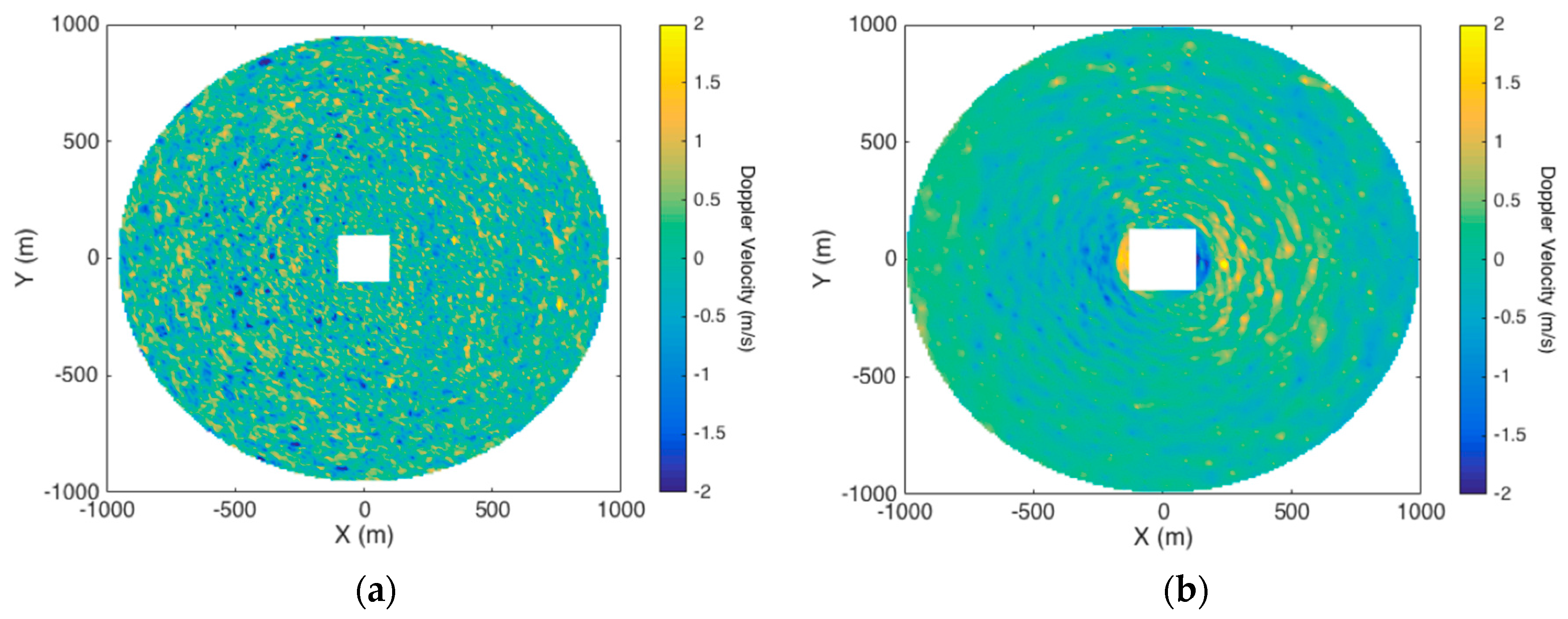
The first radar system was developed by the University of Michigan and The Ohio State University, and from here on will be referred to as the UM system [17]. It is a coherent-on-receive radar and has a center frequency of 9.41 GHz [18]. The antenna rotates at 24 RPM. Pulse-pair processing is used to estimate Doppler velocity [19]. Data is a function of range (r), time (t), and azimuth (ϕ). The Doppler estimates are averaged over 12 pairs for noise reduction, yielding a Doppler velocity range distribution approximately every 0.86° of rotation. The resulting Doppler velocity distribution covers a range of 960 m at a resolution of 3.75 m. One full revolution of the radar system produces one radar frame. A summary of the radar parameters for this system are shown in Table 1. The radar had a blanking range of 100 m around the vessel to eliminate high power return. A sample radar frame is shown in Figure 1a.
The second radar system evaluated was developed by Applied Physical Sciences, Inc. (Groton, CT, USA), which from here on will be referred to as the APS system [20]. This radar uses four coherent antennas mounted at 90° to each other, which rotate at 5 RPM. Each of the four antennas is identical. Each has a center frequency of 9.2 GHz and pulse repetition frequency (PRF) of 25 kHz. Data is a function of range (r), time (t), azimuth (ϕ), and antenna (A). FFT processing [21] is used to produce Doppler estimates over 64 pulses, which yield a Doppler range distribution every 1.23° for a rotation rate of 12 s. One quarter rotation of the system yields a complete frame of data every 3 s because the data from each of the four antennas is combined to generate one frame. The potential advantage of this configuration is that a slower rotation rate permits more pulses to go into each Doppler estimate (referred to as the dwell time), which should make the Doppler estimate more accurate. The tradeoff is that the slow rotation rate can result in aliasing, because the re-visit time to the same patch of ocean surface is longer than many of the ocean surface wave periods. The four antennas mitigate this tradeoff. The resulting Doppler distributions have a range resolution of 4.8 m and cover a range of 998 m. The parameters for this radar system are summarized in Table 1. The radar had a blanking range of 100 m around the vessel to eliminate high power return. A sample radar frame is shown in Figure 1b.
Both of these radars were mounted on ships and collected data during two experiments. The first is referred to as the R/V Melville experiment. This experiment was conducted aboard the R/V Melville from 14–17 September 2013 south of the Channel Islands offshore of Los Angeles, CA. Data were collected across a variety of environmental conditions and at ship speeds of 1–3 m/s. Each radar dataset is approximately 2–3 min in length. During the experiment, 12 GPS mini-buoys developed by the Coastal Observing Research and Development Center at the Scripps Institution of Oceanography, were deployed for use as ground-truth wave sensors [22]. Buoys were deployed from the ship and drifted within and around the radar measurement region. Their positions are geo-referenced to the radar using buoy and ship measured GPS positions. Comparisons consider wave statistics based on a 20-min time series of GPS velocity, and are also averaged over all available buoys at the time of radar data collection.
The second experiment is the Culebra Koa 2015 experiment (CK15). This test took place from 17–21 of May 2015, off the east coast of Oahu, Hawaii. This test was a joint military seabasing exercise featuring the USNS Montford Point, a new class of ship called a Mobile Landing Platform (MLP), made to load and unload cargo from other ships while at sea, and the USNS Dahl, a Watson class Large, Medium-Speed, Roll-on/Roll-off (LMSR) vessel. During the experiment, the radars were mounted on the USNS Dahl, and data were collected across a variety of environmental conditions at ship speeds of 1–3 m/s, where each radar dataset was approximately 2–3 min in duration. Six GPS mini-buoys were deployed and used as ground-truth wave sensors. Buoys were deployed from the ship and drifted within and around the radar measurement region. Their positions are geo-referenced to the radar using buoy- and ship-measured GPS positions. Comparisons consider wave statistics based on a 20-min time series of GPS velocity, and are also averaged over all available buoys at the time of radar data collection. For both experiments, the surface waves are in the deep-water limit of linear wave theory.
In order to evaluate the POD method over various environmental conditions, datasets from both the R/V Melville and CK15 experiments were sub-selected to cover a range of sea states, wind speeds, and wave systems. Sequential datasets from both the APS and UM radars were selected when available in order to evaluate the impact of radar system design on the wave field retrieval method. Datasets were selected to cover a range of small (less than 0.5 m), medium (between 1 m and 2 m), and large (greater than 2 m) Hs for swell dominant, wind wave dominant, and mixed sea states. The Hs conditions measured by the GPS mini-buoys for these experiments ranged from 0.1–2.2 m; thus, the large wave category represents the largest waves observed throughout the course of the two experiments. Representative datasets of the highest and lowest Hs from both experiments are also included in the sub-selected datasets. Swell dominant is defined as having both swell and wind sea spectral peaks, with the larger peak in the swell period band defined as 7–20 s, while wind-wave dominant would have a larger peak in the wind wave period band (2–6 s). Because wind speed, Uw, has a large effect on the signal-to-noise ratio (SNR) of the radar measurement [23,24], the UM and APS datasets from both the R/V Melville and CK15 tests with the smallest and largest Uw are also included in the sub-selection. Wind speeds ranged from 2–15 m/s over the course of the two experiments. Table 2 shows the environmental conditions as measured by GPS wave buoys (Hs, λp and root mean squared (RMS) vertical velocity: Vrms), ship-based anemometer (Uw), and radar (angle between swell and wind waves: Δθ), as well as dataset number, associated test, the date and time of the measurements, the number of wave systems, and which radar system had collected the data. Details regarding the calculation of buoy statistics are explained in Section 4.
3. POD Method
Before the POD wave field extraction method is applied, several pre-processing steps are performed to optimize the POD wave field extraction. The polar Doppler velocity data (D(r, t, ϕ)) is transformed to a Cartesian grid (D(x, y, t)) with 10 m resolution before applying the POD method. Sea clutter measurements are known to be sensitive to the look direction of the radar [25], and it was found that the most accurate results of the POD method were obtained when the wave propagation direction was aligned with the direction of the mode functions (see Equation (2)). Thus, the dominant wave direction is determined from the directional Doppler velocity wave spectrum as well as the time series of radar images due to the 180° directional ambiguity innate to the wavenumber spectrum of an individual radar frame [7]. Subsequently, the data are rotated such that the dominant wave propagation direction is aligned with the x-direction of the Cartesian grid. The data are also linearly detrended along each azimuth to remove currents and ship forward speed. A 700 m range limit is selected in this study to be certain the analysis is limited to high SNR data and all data are equivalent in size. A box around the origin of the size of the radar’s minimum range is blanked with zeros in all directions.
The POD method described here is adapted from Hackett et al. [14], and further details regarding the pre-processing and implementation of the POD method to radar data can be found in Kammerer [26]. The POD method takes a signal, one Doppler velocity radar frame, D(x,y) (or matrix D) in which x and y are spatial coordinates, and decomposes the signal into a series of orthonormal basis functions and spatial coefficients. The basis functions are referred to as modes. The shape of the mode is determined by the data itself, and is not an assumed function a priori. The modes are ranked such that the first mode accounts for the most variance of the signal, the second mode accounts for the second order contributor to the variance, and so on. A summation of all the modes multiplied by the corresponding coefficients results in the reconstruction of the original signal. Thus, if the variance of the Doppler measurement is dominated by ocean surface orbital velocity variation, then one would expect the leading modes to be associated with the wave field. A singular value decomposition is used to perform the POD:
where B, Σ, and P are matrices, and the superscript T indicates matrix transpose. The mode functions are encompassed in P, and the diagonal elements of Σ are the singular values of matrix D. Let Q = BΣ, then,
where qk are the spatial coefficients of the signal (columns of Q), are the basis functions of the Doppler velocity, or the proper orthogonal modes (transposed columns of P), and M is the number of samples in the x-direction. The singular values occur in ranked order along the diagonal elements of Σ and signify the relative importance of each mode.
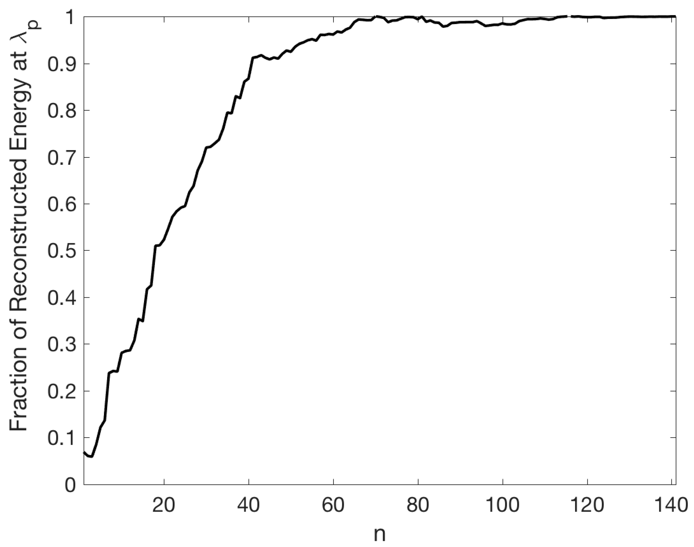
A low-order representation of the signal is obtained by reconstructing the Doppler velocity with a subset of the mode functions and spatial series coefficients (i.e., performing the summation in Equation (2) from k = 1 to n, where n < M). For example, Figure 2 shows the cumulative energy in an increasing number of modes reconstructions (i.e., k = 1 to n), normalized by the total energy (variance) in the radar data at the buoy based peak wavelength. By the 20th mode (14% of all modes), ~50% of the energy is incorporated into the reconstruction (at this wavelength). By 40 modes (28% of modes), 90% of the energy is incorporated, and by ~50% of modes, all of it is present. Equation (2) implies that all the variance at all wavelengths in the original radar measurement is accounted for when all the modes are included. It is unknown exactly what fraction of the variance at the peak wavelength should be attributed to the wavefield, but presumably it should be a large portion. In this study, the selection of the number of modes to use in the reduced-order representation is evaluated, as well as the association of individual modes with physical characteristics of the waves. With proper mode selection, this technique could be used to filter, or extract, the wave field signal from the radar measurements, which also contains contributions from other sources aside from the wave field. Some of these artifacts include: shadowing, “sea-spikes”, interference, wave breaking, and range decay [1,8,25,27,28]. Evaluation of whether or not the mode functions can be used as a filter in this way is a primary objective of this study.
The reconstructed Doppler velocities, based on a sub-selection of modes, are considered phase-resolved wave orbital velocity maps. This procedure is applied to all of the radar frames in the time series (N); thus, the result is a time series of phase-resolved wave orbital velocity maps covering frames 1 to N.
4. Evaluation Statistics
In order to evaluate the accuracy of the wave field extraction method, wave statistics are computed from GPS mini-buoys and from the phase-resolved wave orbital velocity maps produced as described in Section 3. The statistics compared are Hs, Vrms and λp.
Buoy statistics are calculated from a measured time series of GPS velocities from each available buoy during radar data collection times. These data are first high-pass filtered to remove any large-scale variability from the time series, which is typically due to the changing of GPS satellites in time. Vertical velocity data sampled at 1 Hz starting at the time of radar data collection (see Table 2) are used for computing the statistics. Sea surface displacement is calculated by integrating this time series, and an average 1D spectrum is computed from averaged 2-min spectra over 20 min with 50% overlap. Hs and Hs confidence intervals are calculated from this 1D average sea surface elevation spectrum, as described in the National Data Buoy Center manual [29]. The peak wavelength (λp) is found by first converting the frequency spectrum to a wavenumber spectrum using the method outlined in Plant [30], and then locating the wavelength associated with the largest energy in this 1D spectrum. Vrms is the RMS of 2-min segments of filtered vertical GPS velocity time series that are subsequently averaged over ~20 min. Statistics computed for each buoy are averaged over all available buoys.
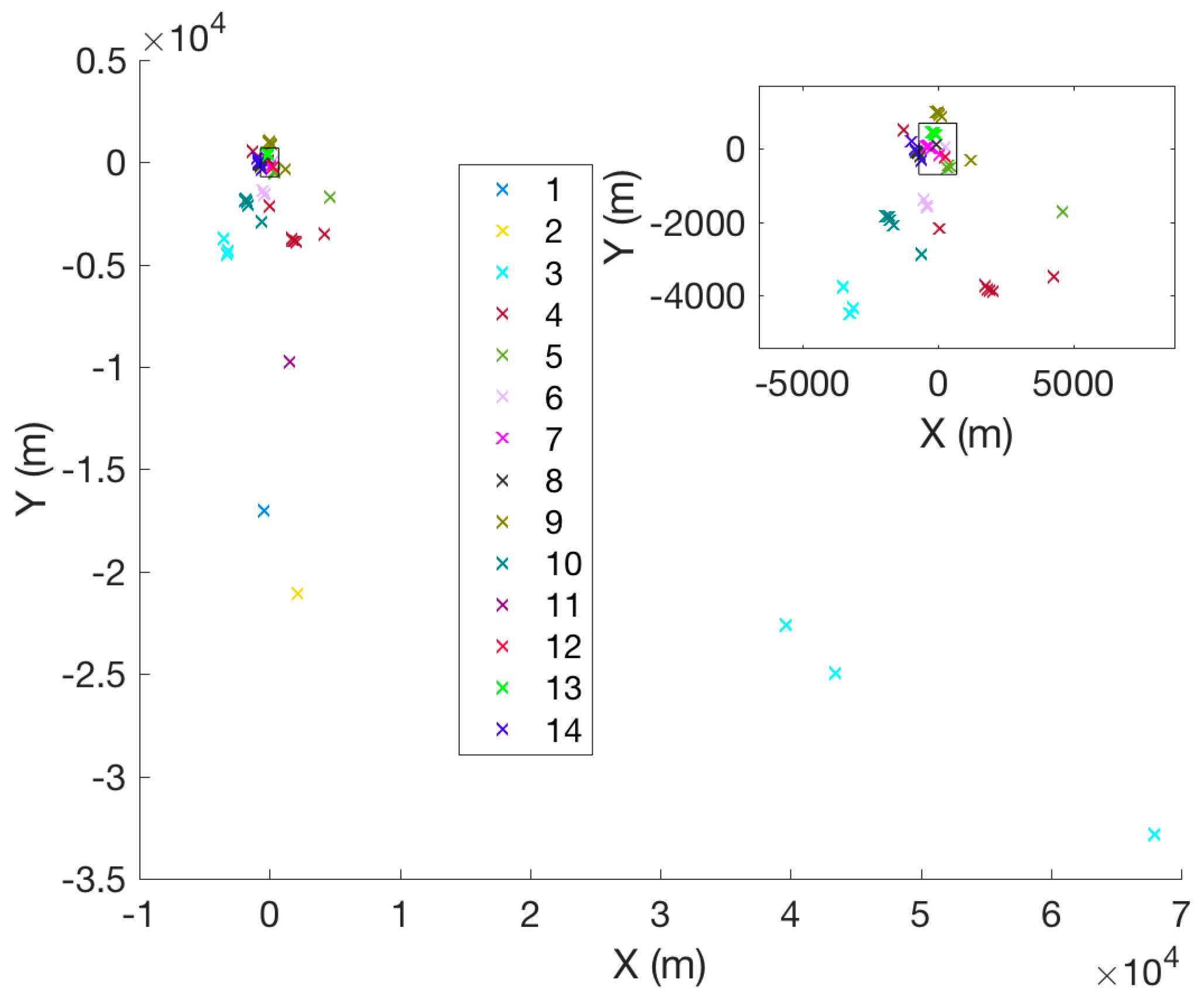
As previously mentioned, the buoys were deployed from the ship each day and drifted around the radar measurement region. Since the buoys and ship were both moving relative to each other at different speeds and directions, it was difficult to consistently keep the buoys within the radar field of view. The amount and location of buoys available for the various radar datasets at the starting time of radar data collection are shown in Figure 3. For most of the datasets, the buoys were either within or very near the analysis region used in this study, denoted by the black square in Figure 3, with the exception of a few buoys from datasets 1–3, and 11. The inset shows a zoom-in of the area near the analysis region.
Wave statistics for rotating radar-extracted wave fields are computed similarly, but from the reconstructed 2–3 min time series of the phase-resolved wave orbital velocity maps. For each orbital velocity map in the time series, statistics are calculated along 1D range transects in the peak wave direction ±5 degrees. Statistics are calculated independently for each transect and then averaged over all of the transects that span ±5 degrees around the peak wave direction. Vrms and λp statistics are computed the same way as described in the previous paragraph for the buoy data, except the conversion from a frequency to a wavenumber spectrum is not needed, because the 1D radar spectrum is already a function of wavenumber. Hs is computed in the same manner as the buoy data, except that the 1D spectrum of vertical velocity is first converted to a sea surface displacement spectrum using the method outlined in Hackett et al. [5] and Hwang et al. [2]. The resulting statistics are then averaged over all of the radar frames in the time series, which covers 2–3 min in duration depending on the dataset.
These statistics are computed along the peak wave direction because Doppler radar measures a projection of the total velocity along the radar look direction; thus, the measured Doppler velocity only contains all of the orbital velocity associated with the dominant wave system along the peak wave propagation direction [3,4]. When two wave systems are present, two different bearings contain the maximum orbital velocity for the wind seas and swell (assuming they are not propagating in the same direction). Thus, we chose to compute the statistics along the radar identified peak wave direction with the understanding that any secondary wave system will only be encompassed as a projection of their orbital velocity along that (primary system) direction. This procedure is also adopted because in the conversion between orbital velocity and wave height, it is assumed that the radar is looking along the wave propagation direction [5].
5. Results and Discussion
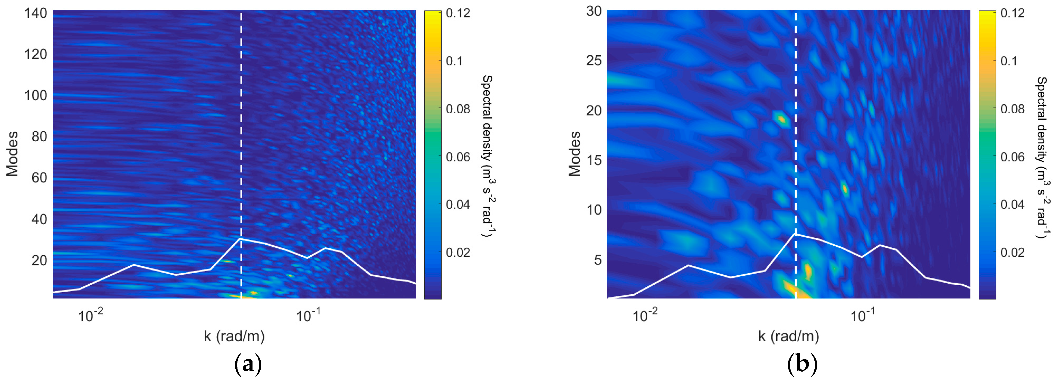
First, we present results demonstrating that the leading POD modes can be associated with the wave field. The POD basis functions obtained from decomposing each radar frame as described in Section 3 results in oscillatory basis functions. To examine the distribution of variance in those basis functions as a function of spatial scale, the 1D spectra of single mode reconstructions are computed. A 2D kx-ky (wavenumber) spectrum is calculated from the individual mode velocity reconstructions and integrated over ky to yield a 1D wavenumber spectrum for each mode reconstruction (between 1 and 141). Each 1D wavenumber spectrum is then compiled to form the spectrogram shown in Figure 4 (for dataset 14). The solid white line is the corresponding average spectrum of all the buoys, and the dashed white line denotes the peak wavelength. The energy contained in mode 1 through mode 10 velocity reconstructions is largest around the peak wavelength, which signifies that a large portion of variance in those mode functions is associated with spatial scales near the peak wavelength of the wave field. The wavelengths associated with concentrated energy peaks in modes below 20 all fall within the wavelengths associated with the highest energy in the buoy spectrum; above 20 modes, small amounts of energy are spread across the remaining reconstructions/modes and across many wavelengths. In other words, aside from some of these leading modes, the variance in the modes is not concentrated at specific length scales. This energy is presumably part of non-wave contributions to the radar Doppler velocity measurement, because it is not directly associated with any known dominant spatial scale of the ocean surface waves. Similar results are found for all of the datasets in Table 2. These results demonstrate that the leading mode functions contain variability associated with the physics of the wave field and suggest that the leading modes can be used to separate wave and non-wave contributions to the radar measurement. These results are consistent with the results shown in Hackett et al. [14], which showed similar trends for simulated idealized radar measurements of synthetic wave fields with a slightly different configuration of the radar data.
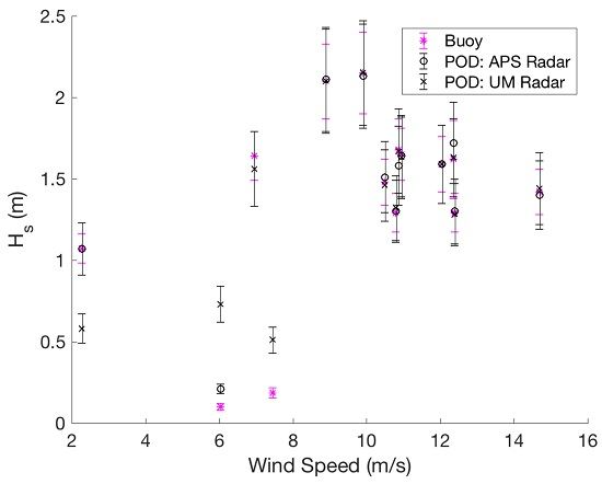
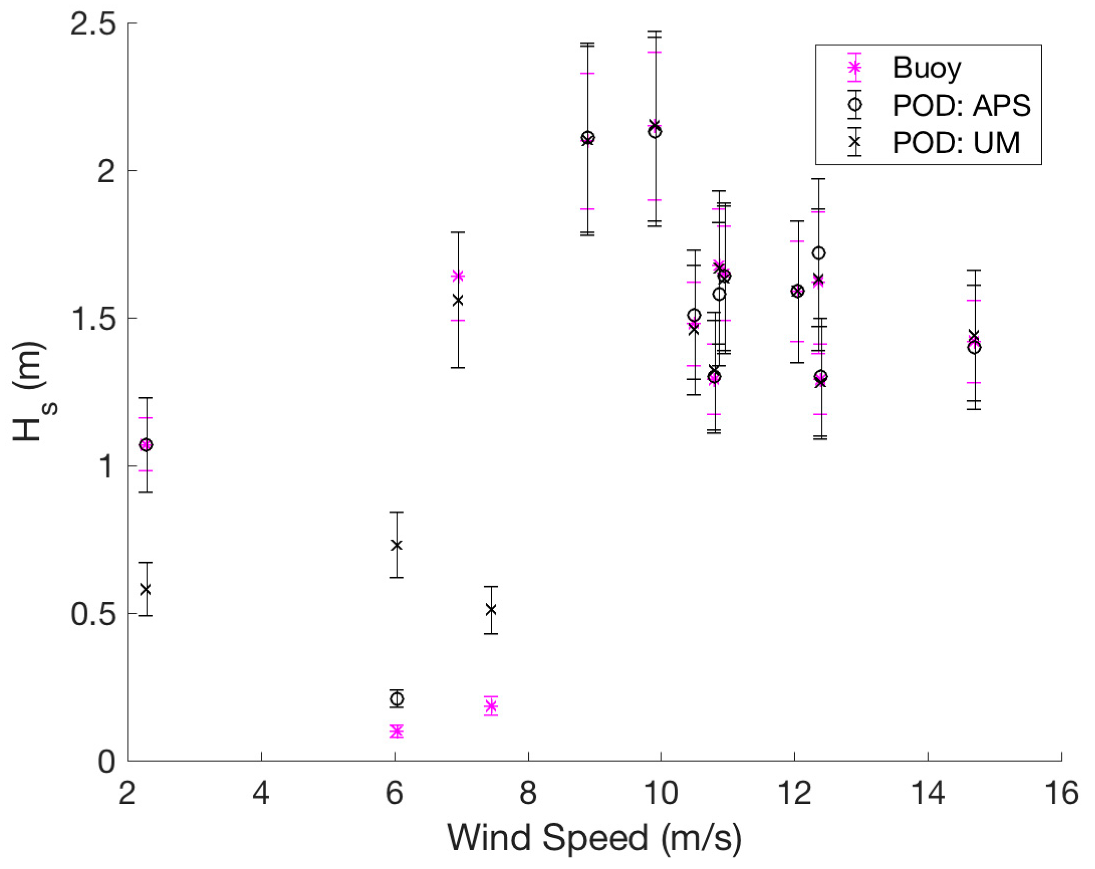
Because the proper mode selection is not straightforward, we computed the Hs statistic for all possible mode reconstructions and determined the mode set that provided the best match to the buoy Hs statistic. This “best mode” is the 1 to n mode reconstruction that results in an Hs that has the closest absolute value compared to the buoy-based Hs. Figure 5 shows the resulting comparison between the buoy-measured Hs and the Hs estimate from the optimal POD mode reconstruction with associated statistical uncertainty (95% confidence intervals). For all datasets but the lowest Hs for the APS radar and the lowest three Hs for the UM radar, the POD Hs estimate falls within the statistical uncertainty of the buoy measurement. These low Hs cases are associated with lower wind speeds, with the exception of one dataset that had a similarly low wind speed (~7 m/s), but a larger Hs, presumably due to the second wave (swell) component. The inaccurate Hs for small waves and low wind speeds is typically due to insufficient Bragg scatterers, and is a common problem with radar-based measurements [2,3,5]. The lowest wind speed case (~2 m/s) was not associated with the lowest wave height case, although only one wave system was present. This finding suggests that the wind speed was decreasing when the dataset was taken. In this case, the APS and UM results differed; applying the POD method on the APS data resulted in a match to the buoy despite the low wind speed, while for the UM data it was underestimated. It is possible that under these difficult conditions, the increased dwell time of the APS radar allows for more accurate Doppler measurements resulting in the more accurate Hs. The results for the second lowest wind speed (~6 m/s) (and lowest Hs) also support this observation; as here, the Hs estimates for the APS radar differ from the buoy less than the results for the UM radar. Overall, the POD method accurately estimates Hs for the majority of the datasets examined. These datasets span a range of environmental conditions; thus, these results appear robust over a variety of environments and differing radar configurations. Figure 6 shows k-ω (wavenumber-angular frequency) spectra for a few sample datasets and the corresponding spectra of the optimally reconstructed orbital velocity maps. Note that most of the energy on the dispersion curve is retained in the reconstructions, but also some energy that is not associated with the linear dispersion relationship. Part of this group line energy (i.e., the linear low frequency feature that lies below the dispersion relationship) has been suggested to be associated with wave interference [8], among other effects such as shadowing, breaking waves, and “sea spikes”.
To obtain the most accurate Hs, different numbers of modes were needed for each dataset. Figure 7 shows the number of modes needed for the “best mode” reconstruction (1 through n) versus the buoy-measured Hs for all of the examined datasets (see Table 2). The UM radar is marked in black dots, and the APS radar in magenta crosses. The majority of datasets are accurately reconstructed by fewer than the leading 20 modes (approximately 15% of the total modes). This result is consistent with the prior result that the basis functions whose variability is dominated by scales associated with the wave field are lower than 20. Note that this low number of modes required for an accurate reconstruction could reduce storage demands for large datasets, because only a subset of the data would need to be retained for the computation of wave statistics. The best mode shows a weak trend with increasing significant wave height, particularly for the UM radar, but there is a large spread. As wave height increases, the complexity of the wave field increases, which might explain this slight increase in the number of required modes to accurately reconstruct the wave field. Importantly, these results also show that the number of modes needed to optimize comparison to the buoy Hs was not uniform over the datasets examined, which indicates variation of the optimal mode number with radar system and environmental conditions.
Figure 8 shows a scatterplot of λp based on the APS and UM POD orbital velocity reconstructions versus the buoy-based values. Peak wavelengths are compared using the buoy identified dominant wave system when two wave systems were present. In such cases (see Table 2), particularly when the two systems were of similar magnitude, the buoy often measured the higher energy on the wind wave peak, while the radar the swell peak. This discrepancy is likely caused by the higher sensitivity of the buoy due to its faster sample rate and higher spatial resolution (small size), especially when the ship had a non-negligible forward speed into the wave propagation direction. The majority of all of the reconstructions are close to the buoy-identified λp, particularly for the UM radar. The APS radar overestimates the wavelengths when the buoy-based peak wavelength is less than around 75 m. This discrepancy may be associated with the higher spatial and temporal resolution of the UM radar measurements, which is the tradeoff with the APS radar that has the longer dwell time, and potentially leads to the increased Hs accuracy in the low wind speeds, as previously discussed. It is noteworthy that although the buoy and radar spectra have similar spectral resolution (but different discrete frequencies), a difference of one point in the identification of the peak wavelength translates to about a 10% error, and across all of the datasets, the peak wavelength identified by the POD reconstruction is generally within one discrete wavenumber point of the buoy spectrum. This result confirms that the POD method is accurately capturing the buoy-identified dominant wave system, and is relatively consistent between the two different radar configurations.
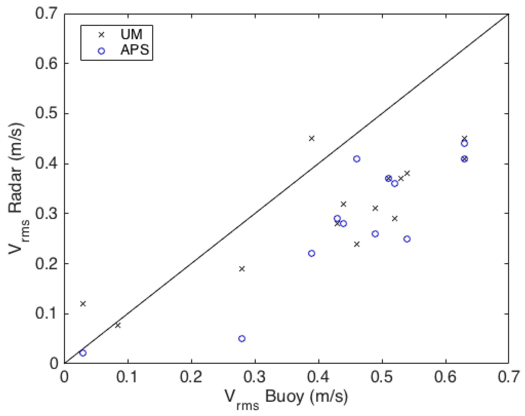
Figure 9 shows a scatterplot of Vrms based on APS and UM POD orbital velocity reconstructions with respect to buoy-measured Vrms. Unlike λp, a significant portion of the data underestimate the Vrms for both radars. The discrepancy between buoy measurements and radar estimations for Vrms is most likely related to differences in velocities measured by the buoy and radar; any wave system component not aligned with the peak direction is underestimated by this approximation of Vrms from the radar data because it only includes a projection of that velocity component onto the peak direction [3,4]. In contrast, the buoy always measures the full magnitude of all of the components simultaneously. Although not shown here, similar discrepancies are also obtained using more conventional processing techniques, i.e., dispersion curve filtering methods [7]. Hence, we conclude that the relatively large errors/bias are not associated with the application of the POD technique to extract the wave field, but with the inherent limitations of the radar measurement [26]. Results from both radars show similar Vrms trends with respect to the buoy.
6. Conclusions and Summary
In this study, an alternative method, POD, for separating ocean surface wave contributions to Doppler radar measurements of the sea surface was examined. POD has a number of potential advantages over conventional FFT-based dispersion filtering for the real-time calculation of wave statistics from Doppler radar measurements of the sea surface. These potential advantages include reduced sampling requirements, the elimination of artifacts from spectral processing and filtering, computational efficiency, and the ability to include non-linear wave energy.
The results show that the lowest POD modes are associated with the physics of the measured wave field, and that wave contributions can be extracted from radar measurements of the ocean surface based on leading modes. The variances of leading mode basis functions are predominantly associated with the spatial scales of the ocean waves. For the majority of the examined datasets with the proper mode selection, wave statistics calculated from POD reconstructions were statistically equivalent to those calculated using GPS wave buoy data independent of radar configuration or examined environmental conditions. Generally, 15% of the total number of modes or fewer was needed to obtain the most accurate Hs.
While this study shows the viability of POD for the extraction of wave information from radar-measured ocean surface Doppler velocity and the calculation of wave statistics, further research into the a priori selection of the proper number of modes without a ground truth sensor is needed. Examination of the dominant spatial scales associated with the basis functions is a first step in determining a means to evaluate mode selection, but more research is needed to evaluate the robustness of such criteria. Furthermore, more research is also needed into determining a method for adjusting for the effect of the projection of sea surface velocity along the look direction of the radar when multiple wave systems exist. It is also noteworthy that there is no obvious reason for why this technique would not also be valid for radar backscatter measurements, and future research should evaluate its use for incoherent radars as well.
Acknowledgments
The authors would like to thank Kevin Cockrell and Jason Rudzinsky from Applied Physical Sciences, Inc. for providing the APS radar system experimental data, Joel Johnson and Shanka Wijesundara from the The Ohio State University for providing the UM radar system experimental data, and Tony DePaulo from the Coastal Observing Research and Development Center at the Scripps Institute of Oceanography for providing the wave data from GPS mini-buoys. We are also grateful to the Office of Naval Research and Paul Hess III for providing the funding for this study (Grant: N00014-15-1-2044).
Author Contributions
Erin E. Hackett conceived and designed the study, and supervised the data analysis. Andrew J. Kammerer analyzed the data. Erin E. Hackett and Andrew J. Kammerer wrote the manuscript.
Conflicts of Interest
The authors declare no conflict of interest.
References
- Nieto Borge, J.C.; Rodriguez, G.R.; Hessner, K.; González, P.I. Inversion of marine radar images for surface wave analysis. J. Atmos. Ocean. Technol. 2004, 21, 1291–1300. [Google Scholar] [CrossRef]
- Hwang, P.A.; Sletten, M.; Toporkov, J. A Note on Doppler processing of coherent radar backscatter from the water surface: With application to ocean surface wave measurements. J. Geophys. Res. Oceans 2010, 115, C3. [Google Scholar] [CrossRef]
- Carrasco, R.; Streßer, M.; Horstmann, J. A simple method for retrieving significant wave height from Dopplerized X-band radar. Ocean Sci. 2017, 13, 95–107. [Google Scholar] [CrossRef]
- Lyzenga, D.R. Polar Fourier transform processing of marine radar signals. J. Atmos. Ocean. Technol. 2017, 34, 347–354. [Google Scholar] [CrossRef]
- Hackett, E.E.; Fullerton, A.M.; Merrill, C.F.; Fu, T.C. Comparison of incoherent and coherent wave field measurements using dual-polarized pulse-Doppler X-band radar. IEEE Trans. Geosci. Remote Sens. 2015, 53, 5926–5942. [Google Scholar] [CrossRef]
- Johnson, J.; Burkholder, R.; Toporkov, J.V.; Lyzenga, D.R.; Plant, W.J. A numerical study of the retrieval of sea surface height profiles from low grazing angle radar data. IEEE Trans. Geosci. Remote Sens. 2009, 47, 1641–1650. [Google Scholar] [CrossRef]
- Young, I.R.; Rosenthal, W.; Ziemer, F. A three-dimensional analysis of marine radar images for the determination of ocean wave directionality and surface currents. J. Geophys. Res. Oceans 1985, 90, 1049–1059. [Google Scholar] [CrossRef]
- Plant, W.J.; Farquharson, G. Origins of features in wave number-frequency spectra of space-time images of the ocean. J. Geophys. Res. Oceans 2012, 117, C6. [Google Scholar] [CrossRef]
- Chatterjee, A. An introduction to the proper orthogonal decomposition. Curr. Sci. 2000, 78, 808–817. [Google Scholar]
- Sirovich, L. Turbulence and the dynamics of coherent structures; part I: Coherent structures. Q. Appl. Math. Comput. 1987, 45, 561–571. [Google Scholar]
- Wyrzkowski, R.; Dongarra, J.; Karczewski, K.; Wasniewski, J. (Eds.) Parallel Processing and Applied Mathematics. In Proceedings of the 9th PPAM International Conference, Torun, Poland, 11–14 September 2011; Springer: Berlin/Heidelberg, Germany, 2012; pp. 569–578. [Google Scholar]
- Smith, S.W. The Scientist & Engineer’s Guide to Digital Signal Processing; California Technical Publishing: San Diego, CA, USA, 1997; pp. 225–242. [Google Scholar]
- Wang, Y.; Yeh, C.; Young, H.V.; Hu, K.; Lo, M. On the computational complexity of the empirical mode decomposition algorithm. Physica A 2014, 400, 159–167. [Google Scholar] [CrossRef]
- Hackett, E.E.; Merrill, C.F.; Geiser, J. The application of proper orthogonal decomposition to complex wave fields. In Proceedings of the 30th Symposium on Naval Hydrodynamics, Hobart, Australia, 2–7 November 2014; p. 9. [Google Scholar]
- Zhang, S.; Song, Z.; Ying, L. An advanced inversion algorithm for significant wave height estimation based on a random field. Ocean Eng. 2016, 127, 298–304. [Google Scholar] [CrossRef]
- Chen, Z.; He, Y.; Zhang, B. An automatic algorithm to retrieve wave height from X-band marine radar image sequence. IEEE Trans. Geosci. Remote Sens. 2017, 1–9. [Google Scholar] [CrossRef]
- Alford, K.; Lyzenga, D.; Beck, R.F.; Nwogu, O.; Johnson, J.T.; Zundel, A. A real-time system for forecasting extreme waves and vessel motions. In Proceedings of the ASME 34th International Conference on Ocean, Offshore, and Artic Engineering, St. John’s, NL, Canada, 31 May–5 June 2015. [Google Scholar]
- Smith, G.E.; O’Briend, A.; Pozderac, J.; Baker, C.J.; Johnson, J.T.; Lyzenga, D.R.; Nwogu, O.; Trizna, D.B.; Rudolf, D.; Schueller, G. High power coherent-on-receive radar for marine surveillance. In Proceedings of the 2013 International Conference on Radar, Adelaide, Australia, 9–12 September 2013; pp. 434–439. [Google Scholar]
- Miller, K.; Rochwarger, M. A covariance approach to spectral moment estimation. IEEE Trans. Inf. Theory 1972, 18, 588–596. [Google Scholar] [CrossRef]
- Connell, B.S.; Rudzinsky, J.P.; Brundick, C.S.; Milewski, W.M.; Kusters, J.G.; Farquharson, G. Development of an environmental and ship motion forecasting system. In Proceedings of the ASME 34th International Conference on Ocean, Offshore, and Artic Engineering, St. John’s, NL, Canada, 31 May–5 June 2015. [Google Scholar]
- Thompson, D.R.; Jensen, J.R. Synthetic aperture radar interferometry applied to ship-generated internal waves in the 1989 Loch Linnhe experiment. J. Geophys. Res. Oceans 1993, 98, 10259–10269. [Google Scholar] [CrossRef]
- Drazen, D.; Merrill, C.; Gregory, S.; Fullerton, A. Interpretation of in-situ ocean environmental measurements. In Proceedings of the 31st Symposium on Naval Hydrodynamics, Monterey, CA, USA, 11–16 September 2016; p. 8. [Google Scholar]
- Rozenberg, A.D.; Ritter, M.J.; Melville, W.K.; Gottschall, C.C.; Smirnov, A.V. Free and bound capillary waves as microwave scatterers: Laboratory studies. IEEE Trans. Geosci. Remote Sens. 1999, 37, 1052–1065. [Google Scholar] [CrossRef]
- Holman, R.; Haller, M.C. Remote sensing of the nearshore. Annu. Rev. Mar. Sci. 2013, 5, 95–113. [Google Scholar] [CrossRef] [PubMed]
- Walker, D. Doppler modelling of radar sea clutter. IEE Proc. Radar Sonar Navig. 2001, 148, 73–80. [Google Scholar] [CrossRef]
- Kammerer, A.J. The Application of Proper Orthogonal Decomposition to Numerically Modeled and Measured Ocean Surface Wave Fields Remotely Sensed by Radar. Master’s Thesis, Coastal Carolina University, Conway, SC, USA, June 2017. [Google Scholar]
- Smith, M.J.; Poulter, E.M.; McGregor, J.A. Doppler radar measurements of wave groups and breaking waves. J. Geophys. Res. Oceans 1996, 101, 14269–14282. [Google Scholar] [CrossRef]
- Raynal, A.M.; Doerry, A.W. Doppler Characteristics of Sea Clutter; Sandia Report (SAND2010-3828); Sandia National Laboratories: Alburquerque, NM, USA, 2010. [Google Scholar]
- Earle, M.D. Nondirectional and Directional Wave Data Analysis Procedures; National Data Buoy Center Technical Document 96-01; U.S. Department of Commerce, National Oceanic and Atmospheric Administration: Slidell, LA, USA, 1996; p. 37.
- Plant, W.J. The ocean wave height variance spectrum: Wavenumber peak versus frequency peak. J. Phys. Oceanogr. 2009, 39, 2382–2383. [Google Scholar] [CrossRef]
Figure 1.
Sample Doppler velocity distributions measured by (a) the UM radar and (b) the APS radar. These Doppler distributions are from dataset 9 for both systems (see Table 2 for details on the environmental conditions). Also note that each frame has been rotated such that the peak wave propagation direction is oriented along the x-axis.

Figure 2.
Energy contained in the 1 to n mode reconstruction at the buoy-based peak wavelength normalized by the total energy in the radar measurement at that wavelength (dataset 14).
Figure 2.
Energy contained in the 1 to n mode reconstruction at the buoy-based peak wavelength normalized by the total energy in the radar measurement at that wavelength (dataset 14).

Figure 3.
The number and location of buoys used for comparison to radar-based wave statistics for the various radar datasets (see legend and Table 2). The points mark the buoy positions at the start of radar data collection for each dataset. The black box denotes the analysis region used in this study, and the inset shows a zoom-in of the area near the analysis region.

Figure 4.
1D wavenumber spectra of individual mode velocity reconstructions versus mode number for the UM radar (dataset 14). Panel (a) shows the full range of proper orthogonal decomposition (POD) modes and panel (b) shows a zoom-in of the leading 30 modes. The solid white line is the corresponding average spectrum of all the buoys amplified by 2000 for (a) and by 500 for (b) for visibility. The white dashed line denotes the peak wavelength.

Figure 5.
Hs estimates with 95% confidence intervals for the radar-based POD method (black) along with buoy-measured estimates (magenta asterisks) for the APS radar (◯) and the UM radar (✖) versus wind speed.
Figure 5.
Hs estimates with 95% confidence intervals for the radar-based POD method (black) along with buoy-measured estimates (magenta asterisks) for the APS radar (◯) and the UM radar (✖) versus wind speed.

Figure 6.
Panels (a–c) show the k-ω spectrum for UM dataset 8, UM dataset 7, and APS dataset 7, respectively. Panels (d–f) show the k-ω spectrum for the POD reconstructions with the most accurate Hs (“best mode”). The linear dispersion relationship for ocean surface waves is shown as the white dotted line for reference.
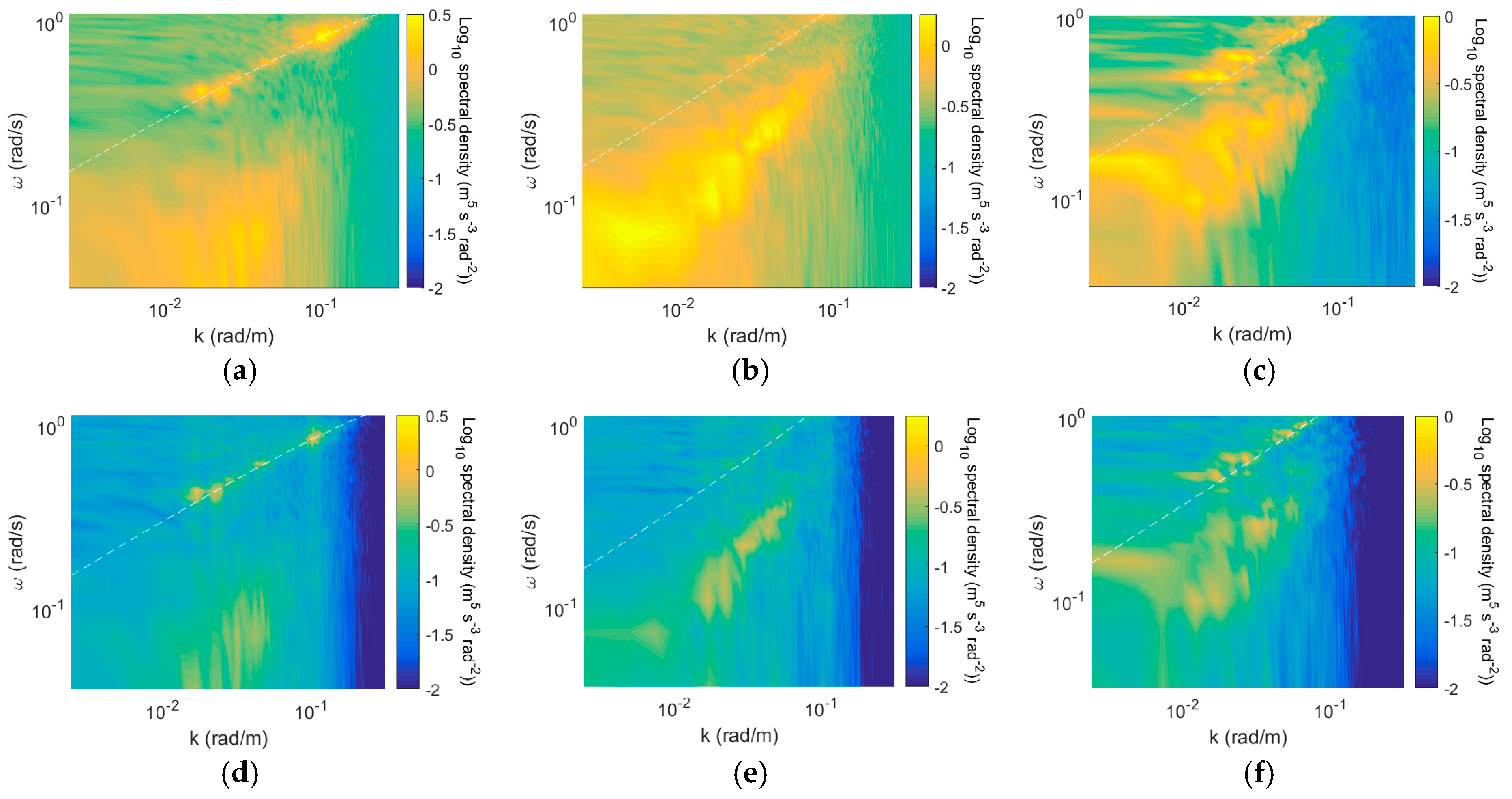
Figure 7.
Most accurate mode with respect to Hs (reconstruction of modes 1 through n) versus buoy measured Hs.
Figure 7.
Most accurate mode with respect to Hs (reconstruction of modes 1 through n) versus buoy measured Hs.
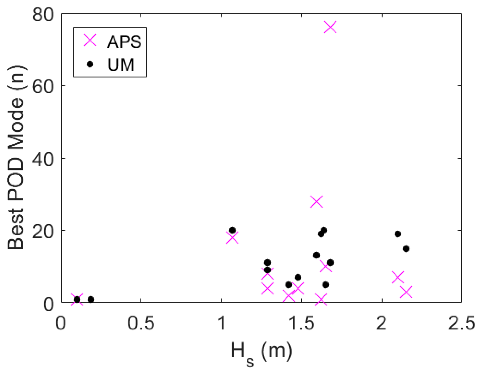
Figure 8.
Scatterplot of λp derived from the APS radar (◯) and UM radar (✖) POD orbital velocity reconstructions versus the buoy-based λp. The dashed line shows the 1:1 line for reference.
Figure 8.
Scatterplot of λp derived from the APS radar (◯) and UM radar (✖) POD orbital velocity reconstructions versus the buoy-based λp. The dashed line shows the 1:1 line for reference.
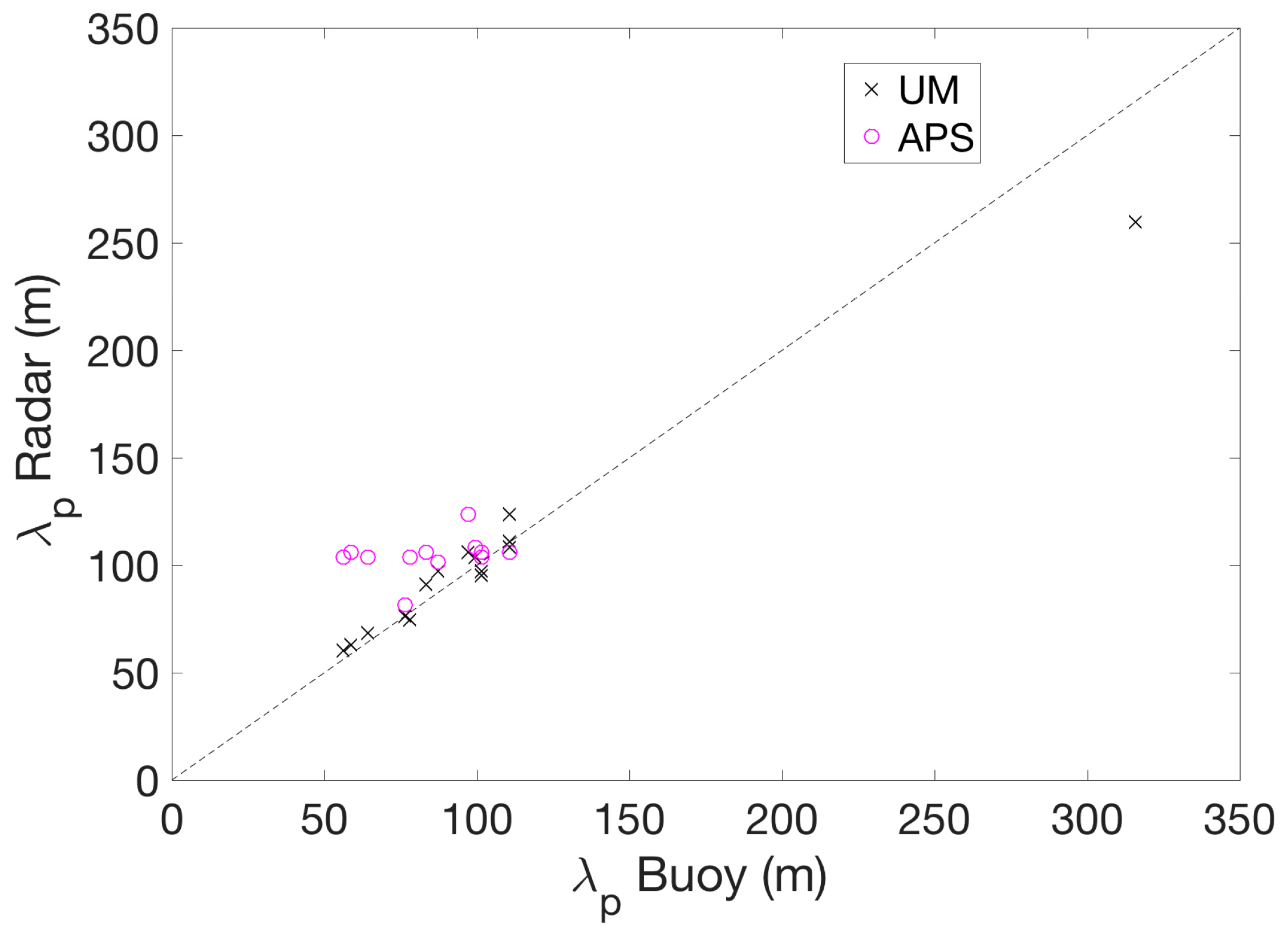
Figure 9.
Scatterplot of Vrms derived from APS radar (◯) and UM radar (✖) POD orbital velocity reconstructions versus the buoy-based Vrms. The solid line shows the 1:1 line for reference.
Figure 9.
Scatterplot of Vrms derived from APS radar (◯) and UM radar (✖) POD orbital velocity reconstructions versus the buoy-based Vrms. The solid line shows the 1:1 line for reference.

Table 1.
Radar parameters: center frequency (fc), bandwidth (Δfb), polarization, resolution, footprint, pulse repetition frequency (PRF), and rotation rate (RPM).
Table 1.
Radar parameters: center frequency (fc), bandwidth (Δfb), polarization, resolution, footprint, pulse repetition frequency (PRF), and rotation rate (RPM).
| Radar System | fc (GHz) | Δfb (MHz) | Polarization | Resolution (m) | Radar Footprint (m) | PRF (Hz) | Rotation Rate (RPM) |
|---|---|---|---|---|---|---|---|
| UM | 9.41 | 30 | VV | 3.75 | 960 | 2000 | 24 |
| APS 1 | 9.20 | 28 | VV | 4.80 | 998 | 25,000 | 5 |
1 one of the four APS antennas.
Table 2.
Datasets sub-selected for this study from the R/V Melville and CK15 experiments and the associated range of environmental conditions covered. Hs, λp and Vrms were measured using GPS mini-buoys. Uw was measured using a ship-mounted anemometer. Δθ was calculated from the radar measured directional wave spectrum. The dataset number, associated test, date and time of the measurements, number of wave systems, and which radar system had collected data at this time are also provided.
| Dataset | Test | Date | Time | APS | UM | Hs (m) | Uw (m/s) | λp (m) | Vrms (m/s) | Wave Systems | Δϴ (°) |
|---|---|---|---|---|---|---|---|---|---|---|---|
| 1 1 | CK15 | 17 May 2015 | 20:08:00 | ✓ | ✓ | 0.10 | 6.0 | 167 | 0.03 | 2 | 53 |
| 2 4 | CK15 | 17 May 2015 | 21:20:00 | ✕ | ✓ | 0.19 | 7.5 | 111 | 0.09 | 1 | 0 |
| 3 | Melville | 15 September 2013 | 17:10:40 | ✓ | ✓ | 1.62 | 12 | 105 | 0.39 | 1 | 0 |
| 4 4 | Melville | 16 September 2013 | 1:36:00 | ✓ | ✓ | 1.42 | 15 | 95 | 0.46 | 1 | 0 |
| 5 1 | Melville | 16 September 2013 | 15:43:00 | ✓ | ✓ | 1.29 | 11 | 82 | 0.43 | 2 | 23 |
| 6 1 | Melville | 16 September 2013 | 18:29:32 | ✓ | ✓ | 1.29 | 12 | 98 | 0.44 | 2 | 50 |
| 7 | Melville | 17 September 2013 | 0:08:45 | ✓ | ✓ | 1.65 | 11 | 77 | 0.54 | 2 | 41 |
| 8 | Melville | 17 September 2013 | 0:33:34 | ✓ | ✓ | 1.48 | 11 | 78 | 0.49 | 2 | 46 |
| 9 | Melville | 17 September 2013 | 0:58:10 | ✓ | ✓ | 1.68 | 11 | 78 | 0.52 | 2 | 44 |
| 10 | Melville | 17 September 2013 | 2:00:00 | ✓ | ✓ | 1.59 | 12 | 92 | 0.51 | 2 | 30 |
| 11 2 | CK15 | 17 May 15 | 22:20:00 | ✕ | ✓ | 1.64 | 7.0 | 111 | 0.53 | 2 | 61 |
| 12 3 | CK15 | 21 May 15 | 20:32:00 | ✓ | ✓ | 1.07 | 2.3 | 97 | 0.28 | 1 | 0 |
| 13 3 | Melville | 17 September 2013 | 14:28:53 | ✓ | ✓ | 2.10 | 8.9 | 108 | 0.63 | 2 | 59 |
| 14 2 | Melville | 17 September 2013 | 19:27:33 | ✓ | ✓ | 2.15 | 9.9 | 105 | 0.63 | 2 | 0 |
1 Lowest Hs for respective test; 2 Highest Hs for respective test; 3 Lowest Uw for respective test; 4 Highest Uw for respective test.
© 2017 by the authors. Licensee MDPI, Basel, Switzerland. This article is an open access article distributed under the terms and conditions of the Creative Commons Attribution (CC BY) license (http://creativecommons.org/licenses/by/4.0/).
Share and Cite
MDPI and ACS Style
Kammerer, A.J.; Hackett, E.E. Use of Proper Orthogonal Decomposition for Extraction of Ocean Surface Wave Fields from X-Band Radar Measurements of the Sea Surface. Remote Sens. 2017, 9, 881. https://doi.org/10.3390/rs9090881
AMA Style
Kammerer AJ, Hackett EE. Use of Proper Orthogonal Decomposition for Extraction of Ocean Surface Wave Fields from X-Band Radar Measurements of the Sea Surface. Remote Sensing. 2017; 9(9):881. https://doi.org/10.3390/rs9090881
Chicago/Turabian StyleKammerer, Andrew J., and Erin E. Hackett. 2017. "Use of Proper Orthogonal Decomposition for Extraction of Ocean Surface Wave Fields from X-Band Radar Measurements of the Sea Surface" Remote Sensing 9, no. 9: 881. https://doi.org/10.3390/rs9090881
Note that from the first issue of 2016, this journal uses article numbers instead of page numbers. See further details here.