
Reducing the Effect of the Endmembers’ Spectral Variability by Selecting the Optimal Spectral Bands


Department of Photogrammetry and Remote Sensing, Faculty of Geodesy & Geomatics Engineering, K. N. Toosi University of Technology, Tehran 19967-15433, Iran
*
Author to whom correspondence should be addressed.
Remote Sens. 2017, 9(9), 884; https://doi.org/10.3390/rs9090884
Submission received: 6 June 2017
/
Revised: 19 August 2017
/
Accepted: 23 August 2017
/
Published: 25 August 2017
(This article belongs to the Special Issue Hyperspectral Imaging and Applications)
Abstract
:Variable environmental conditions cause different spectral responses of scene endmembers. Ignoring these variations affects the accuracy of fractional abundances obtained from linear spectral unmixing. On the other hand, the correlation between the bands of hyperspectral data is not considered by conventional methods developed for dealing with spectral variability. In this paper, a novel approach is proposed to simultaneously mitigate spectral variability and reduce correlation among different endmembers in hyperspectral datasets. The idea of the proposed method is to utilize the angular discrepancy of bands in the Prototype Space (PS), which is constructed using the endmembers of the image. Using the concepts of PS, in which each band is treated as a space point, we proposed a method to identify independent bands according to their angles. The proposed method comprised two main steps. In the first step, which aims to alleviate the spectral variability issue, image bands are prioritized based on their standard deviations computed over some sets of endmembers. Independent bands are then recognized in the prototype space, employing the angles between the prioritized bands. Finally, the unmixing process is done using the selected bands. In addition, the paper presents a technique to form a spectral library of endmembers’ variability (sets of endmembers). The proposed method extracts endmembers sets directly from the image data via a modified version of unsupervised spatial–spectral preprocessing. The performance of the proposed method was evaluated by five simulated images and three real hyperspectral datasets. The experiments show that the proposed method—using both groups of spectral variability reduction methods and independent band selection methods—produces better results compared to the conventional methods of each group. The improvement in the performance of the proposed method is observed in terms of more appropriate bands being selected and more accurate fractional abundance values being estimated.

1. Introduction
In the past decade, numerous methods have been introduced for unmixing hyperspectral imagery [1,2]. Spectral mixture analysis (SMA) is one of most commonly-used methods, and is used in different applications. Basically, the spectra of mixed pixels are modeled using linear or non-linear mixture models. The spectral signature of each pixel is converted to a set of fractional abundances of its constituent spectra (endmembers) by these models [3]. The answer to this question of which one (linear or non-linear models) is superior for unmixing the hyperspectral data is not clear, and depends on the type of the mixture of objects and their applications. However, the acceptable accuracy and the simplicity of linear mixture models entice more researchers to employ them [4]. If the multiple scattering among the endmembers is negligible and the mixture could be supposed macroscopic, a linear mixture model (LMM) can be written as Equation (1):
where is the vector of observations; B is the number of bands; is the index of pixels in the image; is the spectral signature of endmembers; p is the number of endmembers; is the abundance of the ith endmember in the nth pixel; is the coefficient matrix of endmembers; is the vector of abundance values in the nth pixel; and represents noise.
The accuracy of the unmixing process highly depends on the completeness and goodness of the selected endmembers. Therefore, many endmember extraction algorithms have been developed in recent years [3,5]. The accuracy of the fractional abundances obtained from SMA is affected by the residual spectral error caused by inaccurate atmospheric correction, an insufficient signal-to-noise ratio (SNR), and the noise caused by neglecting the non-linear effect of inputs. However, the most important source of error in SMA is due to ignoring the spectral variability (SV) of endmembers caused by variable illumination and environmental, atmospheric, and temporal conditions [4]. These algorithms generally model the entire image using a constant spectral feature for each endmember. In fact, this is a simplification, because in many cases the spectrum of endmembers could change in different spatial and temporal conditions.
Generally, two types of SV can be distinguished among the samples from different classes: (1) the variability within the endmembers of a specific class (intra-class variability); and (2) the spectral similarity between the endmembers of different classes (inter-class variability) [4]. By increasing the intra-class variability, the accuracy of sub-pixel fraction estimation decreases linearly [6]. On the other hand, in some applications where the separation of similar phenomena is of interest, the spectral similarity among the different endmembers (e.g., crops and weeds in agricultural fields or spectral similarity among minerals) makes it difficult to separate these classes. The estimation of the fractional abundances using the linear mixture model could be achieved by different methods, such as least squares and sparse regression with different constraints [3,7]. In the least squares-based spectral unmixing problem, the spectral similarity among the endmembers results in a high correlation between the columns of the coefficients matrix (M) in Equation (1). Consequently, the rank deficiency of the coefficients matrix leads to an unstable solution for the least squares problem and decreasing the accuracy of the estimation of the fractional abundances. Despite the serious effects in the LMMs and the destruction of the reliability of the results of spectral unmixing (SU), this issue is typically ignored [8].
According to [4], the efforts to decrease the effect of the SV can be classified into five general categories: (1) the use of multiple endmembers for each component in an iterative mixture analysis procedure; (2) the spectral weighting of bands; (3) the spectral transformations; (4) the use of radiative transfer models in a mixture analysis; and (5) the selection of a subset of stable spectral features. In addition, to significantly improve the accuracy of the estimation of fractional abundances, the last strategy effectively reduces the computational cost.
The non-orthogonality of the endmembers appears when a linear correlation exists between two endmembers or a multi-collinearity exists among some endmembers. By increasing the correlation among the endmembers, the LMM tends to be instable and extremely sensitive to the small variations of the input spectrum and noises. According to [8], the approaches to deal with the problem could be categorized as: (1) excluding the correlated endmember; (2) de-correlating the endmembers using the spectral transformations; (3) using iterative approaches to select the independent endmembers; and (4) the regularization of the SU equations. Regarding the redundancy of bands in the hyperspectral images, it is not unexpected to identify a subset of bands that decreases the correlation of endmembers. To deal with the problem, the correlation of endmembers can be evaluated using singular value decomposition (SVD) and the condition number of the coefficient matrix of the endmembers in the unmixing procedure.
This paper presents a novel and effective approach for managing the SV and decreasing spectral correlation among the endmembers based on the selection of the optimal bands in the Prototype Space (PS) [9]. The proposed method consists of two main steps. Based on the spectral behavior of the endmembers’ set, the image bands are firstly prioritized in such a way that they have the least sensitivity to the SV of the endmembers. Then, the optimal band selection is done based on this prioritization. Since the spectral correlation among the image bands is not considered in this process, in the second step the independent bands are selected using their angles in the PS. In this way, the spectral correlation among the endmembers is reduced as well. Besides, collecting a spectral library from the SV of endmembers is an expensive and time-consuming process. Therefore, these sets were directly extracted from the image in this paper.
The remaining parts of the paper are organized as follows: the theoretical background and the previous algorithms are introduced in Section 2; the proposed method is explained in Section 3; the experimental results and further discussion are provided in Section 4; and concluding remarks are found in Section 5.
2. Theoretical Background
The effect of the SV of endmembers in the SU and the approaches developed to deal with it have been taken into consideration in [4,10,11]. Furthermore, the problems caused by the spectral correlation among the endmembers and its adverse effects on the reliability of the results of the SU have been investigated in [8]. Given the centrality of the optimal band selection to enhancing the stability of the elected set against the spectral variation and also to decrease the spectral correlation among the endmembers in the proposed method, the algorithms that have dealt with the problem by the band selection approach are reviewed in this section.
2.1. Feature Selection Algorithms to Decrease the Spectral Variability Effect
The precise selection of bands that are stable against the SV (e.g., those bands that minimize the intra-class variance and maximize the inter-class dispersion) plays a significant role in the accuracy improvement of the estimation of fractional abundances. Previous studies on the variability of the optical properties of leaf, litter, and soil in semi-arid and arid areas had illustrated that the SWIR2 region from 2050–2500 nm is the least dependent on variations in structural and biochemical attributes [12]. Therefore, this region was selected as a stable spectral region for the aforementioned materials to be used in the SMA for developing the AutoSWIR algorithm in [12]. However, since the position and the spectral region of bands, as well as the number of stable spectral regions depend on the spatial, spectral, and temporal complexity as well as the mixture of endmembers that are present in the scene [4], this algorithm was not extendable for different ecosystems.
In [13], a more applicable spectral feature selection algorithm entitled the stable zone unmixing (SZU) was introduced. In this algorithm, the sensitive wavelengths to the SV are evaluated using the instability index (ISI). Then, a protocol was introduced to enhance the spectral subset selection by accounting for a tradeoff between the number of wavelengths used in the analysis (i.e., information) and the ISI (i.e., spectral variability).
The redundancy problem of the hyperspectral images and high correlation between their bands was not taken into account in either of the methods (AutoSWIR and SZU). A greater potential in computation efficiency and fraction estimate accuracy could only be provided if the independent bands were employed in the LMM [4].
2.2. Feature Selection Algorithms to Decrease the Spectral Correlation of Endmembers
The most common way to deal with the correlation of endmembers is to eliminate the collinear endmembers [8], which causes two disadvantages: (1) If two endmembers are highly correlated, which one should be excluded? (2) When an endmember is eliminated, it may contain some useful information that could result in destabilizing the LMM. Another solution is to combine the two correlated classes to form a new endmember. However, this will inevitably result in missed classes or similar problems to exclude the endmembers. There are a number of transformations (e.g., principal component analysis (PCA) [14] and the maximum noise fraction (MNF) [15]) which can be employed to reduce the correlation of endmembers by de-correlating the band-to-band correlation. The major drawback of these methods is encountering endmembers whose spectral response has no physical meaning [8].
Another obvious solution that comes to mind is to use a number of subsets of the spectral region. Regarding the high spectral resolution of the hyperspectral images, the spectral region could be decomposed into the visible, near-infrared, and shortwave infrared sections. Then, only those regions that contain the absorption features of the objects of interest could be employed in the appropriate applications. Of course, different regions of the electromagnetic wave spectrum have been theoretically considered by researchers in order to examine different phenomena (i.e., using the shortwave infrared region for analyzing minerals). However, upon decreasing the spectral region, the correlation among endmembers increases [8].
Recently, several endmember-extraction-based methods were applied to feature selection methods, which elect the distinctive spectral signatures. Some of these methods (e.g., geometrical feature selection (G-FS) [16] and linear prediction (LP) [17]) operate in the pixel space. The dimensionality of such a space is equal to the number of participating image pixels. Some others, such as prototype feature selection (PFS) and maximum tangent discrimination (MTD) [18] extract informative bands in an unsupervised manner via geometrical interpretation of distinctive bands in the Prototype Space (PS) [9]. In this way, the axes of the PS are defined based on the spectrum of the extracted endmembers or the clusters’ center of the existing classes in the scene. Therefore, the dimensionality of such a space is equal to the number of constructive components of the scene, and each band is represented as a point or vector in this space. Using these methods, a subset of independent bands that are distributed throughout the spectral region of the hyperspectral sensor could be provided by eliminating the dependent bands in a meaningful manner.
2.2.1. Quantitative Evaluation of the Endmembers’ Correlation
In order to quantitatively estimate the correlation of endmembers constructing the coefficient matrix (M), two measures can be employed [8]: (1) deriving a measure from the coefficient matrix based on its singular values, and (2) extracting a measure from the correlation of the endmembers’ spectra. The SVD of the endmembers matrix (M) to extract singular values (i.e., the square root of eigenvalues) is M = U ∑VT, where U and V are both square, unitary, and orthonormal matrices, and ∑ is a diagonal matrix with the singular values of M. The ratio of the largest singular value to the smallest one is called the condition number of the matrix. The ideal value of one for the condition number indicates that the matrix is fully orthogonal. By increasing the condition number of the endmember matrix, the correlation of endmembers increases, and in an extreme case, will cause the singularity of the matrix. If the correlation of endmembers exceeds 0.6, the condition number increases exponentially [8]. In this way, the condition number is a good measure to evaluate the endmembers’ correlation.
The correlation matrix of the endmembers partially shows the collinearity of each pair of endmembers. The average value of the upper or the lower triangle elements of the matrix provides a measure that indicates the average correlation of the endmembers constructing the coefficient matrix, and could be used as a measure of the overall correlation of endmembers.
3. The Proposed ISI-PS Method
This section explains the proposed ISI-PS method, which is an incorporation of the methods to decrease the SV effect and to select the independent bands of the hyperspectral images. These two factors directly play a positive role in enhancing the accuracy and the reliability of the fractional abundances computed. The proposed method has been developed by assuming the existence of some pure pixels in the image for each class.
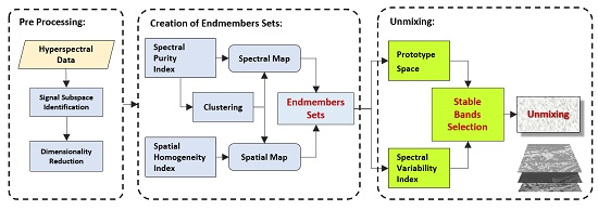
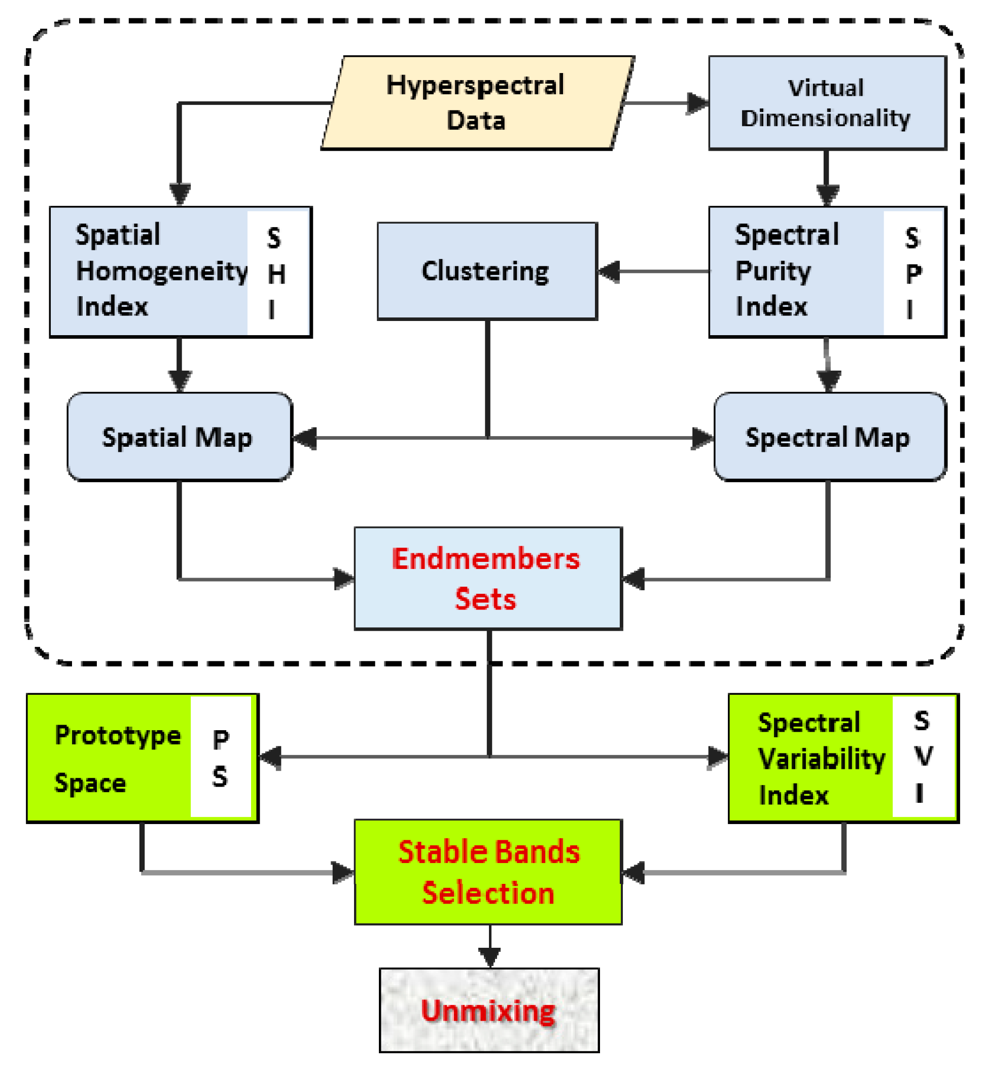
In order to explain the relation of the different parts of the proposed method, its flowchart (Figure 1) and pseudo-code are presented, and detailed information is provided in the following sections. By assuming the existence of pure pixels in the hyperspectral images, a set of pure spectra is firstly provided for each class, which indicates the class spectral variability. These sets are employed to create the endmember of each class and statistical analysis in each band. In this way, the extraction of the information of the endmembers in the proposed method has been compiled based on the geometrical endmember extraction algorithms and by assuming the existence of pure pixels in the image. By means of intra-class and inter-class analysis using measures (e.g., ISI) that consider the SV, the persistent bands against the variability are prioritized. Thereafter, the PS is established based on the spectra of the pure representative of each class, and then bands are represented in this space. Finally, the correlation among the prioritized bands is measured by computing their angles in the PS, and then those that have a similar behavior are eliminated. Thus, the remaining bands are independent and persistent against the variability, which are employed to do the SU and estimate the fractional abundance of each endmember.
Pseudocode of the proposed method:
- (1)
- Estimating the number of classes of the image and establishing a spectral library of the SV of endmembers (i.e., the sets of endmembers).
- (2)
- Prioritizing the persistent bands against the SV using the SV index and some training data.where Ω is the set of prioritized persistent bands (B) and ith is the prioritizing index of bands.
- (3)
- Selecting the most different bands in the PS using the distance of the bands from the main diagonal of the space, .
- (4)
- Considering band and computing its angle from all members of set in the PS.
- (5)
- If the angle of band from all of the previously selected bands was greater than a predefined threshold (T), then ; otherwise, , and band is eliminated.
- (6)
- Unmixing the hyperspectral image using the selected bands.
3.1. Establishing a Set of Spectral Variabilities for Each Endmember
The LMM is widely used to model the spectral composition of a spectrum. However, many reasons lead to the SV of endmembers, such as the change of environmental illumination, as well as atmospheric and temporal conditions [10]. The methods for dealing with the endmembers’ variability could be categorized into two classes [10]: (1) endmembers as sets, and (2) endmembers as statistical distributions. Usually, methods of the first category require a spectral library of the SV of endmembers to deal with the variability phenomena. Collecting a spectral library of the endmembers’ variabilities is an expensive and time-consuming process. Therefore, automatic extraction of endmembers’ sets from an image is greatly beneficial. In this regard, automated endmember bundles (AEB) [19] has established endmembers sets by executing standard endmember extraction algorithms such as N-FINDR [20], orthogonal subspace projection (OSP) [21], unsupervised fully constrained least squares (UFCLS) [22], iterative error analysis (IEA) [23] and vertex component analysis (VCA) [24] and clustering the resulted endmembers from different methods. Recently, the authors in [25] showed that VCA is essentially the same as simplex growing algorithm (SGA) [26] as long as their initial conditions are the same. So, other conventional endmember extraction algorithms such as SGA can be used in AEB.
Spectral features of those spectra that are located in each endmember set indicate the representative of that endmember. Obviously, it is due to the SV that these features are not exactly similar. Therefore, these representatives should have the general condition of an endmember, including: (1) they should lie next to the vertex of point clouds in the feature space; (2) they should situate in homogenous regions in the spatial domain; and (3) pixels of each class should have a similar spectral behavior. Recently, a module entitled spatial–spectral preprocessing (SSPP) was presented in [27], which could be used as a preprocessing function prior to endmember identification and SU. This module firstly computes the spatial homogeneity index for the pixels of the image, which is used to determine the homogenous regions of the image. Simultaneously, unsupervised clustering is employed to identify the spectral classes. Finally, by fusion of this spatial and spectral information, a subset of pixels that are spatially homogenous and spectrally pure is identified in each class, which could be used as the input of the endmember extraction algorithms.
In this way, the applied procedure to determine the endmembers has been shown in the dashed box of Figure 2 and runs as follows. Firstly, the virtual dimensionality (VD) of the image (p) is determined via Hysime [28]. Thereafter, the dimension is reduced using a PCA or MNF transformation into (p-1) bands. In this reduced feature space, endmembers are found via the well-known pixel purity index (PPI) [29] technique with a threshold value equal to zero. Then, the obtained results from the PPI are clustered into p clusters. Instead of the common K-means clustering (which is suitable for classes with spherical distributions), the Fast Density Peak Detection (FDPC) method [30] is applied since herein the classes are seen to have a variety of different distributions. Since the endmembers are found, image homogeneous regions are also detected by a Gaussian filter, and according to Equations (6) and (7). The previously found endmembers are prioritized according to both their spectral purity and homogeneity indices. Next, the spatial and spectral maps are generated based on the first 20% of the purest pixels, as well as 30% of the most homogeneous ones. The ultimate representative endmembers of each class are finally selected from the overlap of these two maps.
3.2. Reducing the Spectral Variability Effect by Selecting the Optimal Bands
In contrast with the conventional SMA methods which use the overall spectral region (i.e., all bands), SZU [13] has been designed based on the selection of persistent bands against the SV phenomena using ISI. The numerical value of this index is computed using Equation (2), which has been developed based on the Fisher separability function. This index is defined for each band based on the ratio of the intra-class dispersion (i.e., the total standard deviation of endmembers for each class) to the inter-class variability of endmembers (i.e., the average distance among the center of classes). The value of one indicates that the intra-class and inter-class variations are similar, and the smaller this value, the better the situation for that band to separate classes.
where p is the number of endmembers and and are the standard deviation and the average of class i in the band λ, respectively. The image’s bands could be prioritized with respect to the SV of their constituent spectra using this index.
3.3. Reducing the Correlation of Endmembers by Selecting the Independent Bands in the Prototype Space
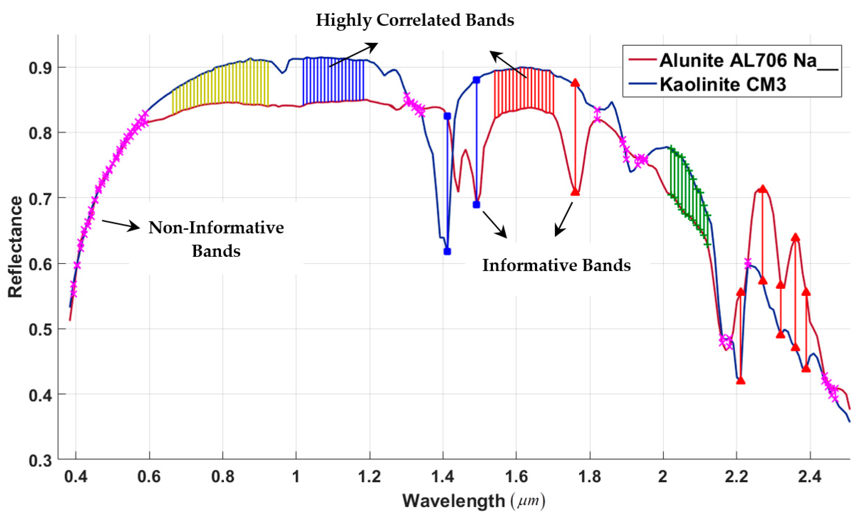
Linear correlation of two or more endmembers always exists in the SU of hyperspectral images. However, little attention has been paid to this [8]. One of the main objectives of this paper is to reduce these correlations without the elimination of the dependent endmembers. This is because—as was mentioned—it would be of interest to separate the different species in some applications. On the other hand, the correlation of the spectrum of endmembers’ sets for adjacent bands has not been considered in the band prioritizing process to reduce the effect of the SV. These two issues are closely related to each other. Therefore, by eliminating those bands for which the endmembers’ sets spectrum is similar, the less-correlated spectral features of these endmembers could be achieved. The spectrum of alunite and kaolinite minerals from the USGS spectral library is represented by the spectral response of the AVIRIS sensor in Figure 2. As can be seen, the bands in the blue, red, and yellow regions are redundant. Besides, these regions may be correlated with each other.
In order to estimate the correlation of bands, some methods have been proposed based on the divergence and correlation functions on the histogram of the image’s bands [31,32]. However, since the goal is to improve the condition of the coefficient matrix to reduce the endmembers’ correlation, in this paper, the angle of bands in the prototype space has been used as a measure of the correlation of endmembers’ sets in those two bands. In other words, by establishing the PS using the endmembers and representing the bands in this space, the dependent bands could be identified. The advantage of this method is that the correlation of bands is evaluated dealing with the endmembers’ sets, because the axes of the PS are the endmembers. Therefore, if the combination of the endmembers is changed in the scene, the proposed method will select a new subset of bands that also have the minimum correlation.
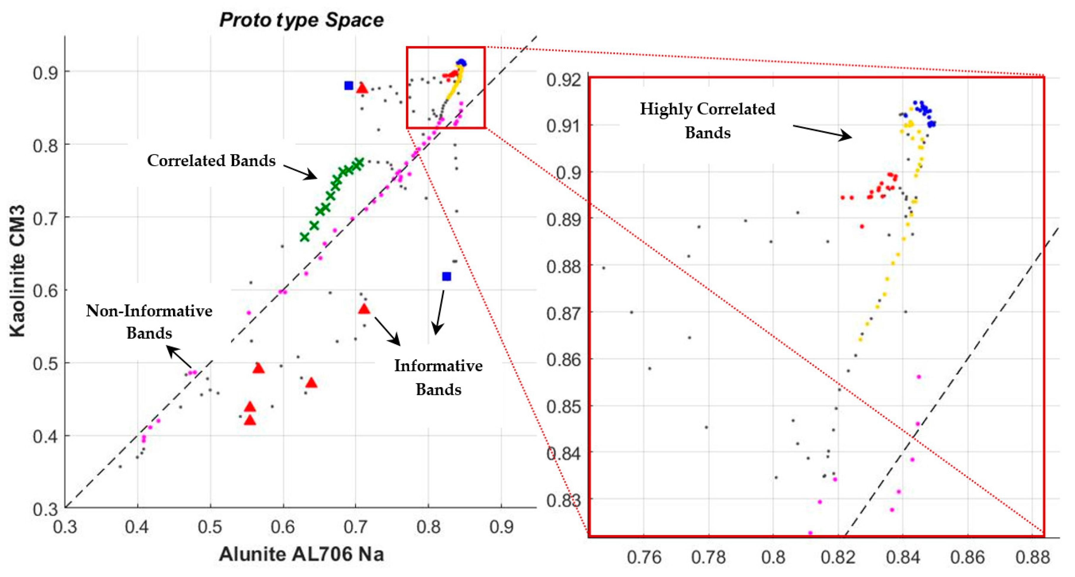
Bands are categorized into three classes in the PS: (1) informative bands: the lager the distance of bands from the main diagonal of the space, the better the bands can separate the image’ classes; (2) correlated bands: the bands that have a similar spectral response of endmembers are gathered close together in this space—this concept is beyond the correlation of the adjacent bands in the hyperspectral images, because it would have occurred for those bands that are not adjacent; (3) non-informative bands: those bands that are located close to the main diagonal of the space, which have the exact same response for different classes [9].
The spectrum (i.e., bands) of alunite and kaolinite minerals (Figure 2) are illustrated in the PS, which was constructed based on these two endmembers in Figure 3. In this figure, examples of highly correlated bands (using blue, red, and yellow colors, which are shown with magnification in the right view), informative bands (the two bands that are shown with blue squares and that have the largest distances from the main diagonal of the space, and those bands that are illustrated with red triangles in which the two spectra have an appropriate distance from each other) and uninformative bands (those bands that are shown with magenta color and that are located close to the main diagonal of the space) are illustrated.
It is obvious that the angles of the correlated bands are close to each other, even if these regions with a similar spectrum are not adjacent. Therefore, the correlation of bands in dealing with the endmembers could be understood by extracting these angles.
3.4. Determining the Threshold Value to Identify the Independent Bands
A threshold value should be defined in order to identify and eliminate the correlated bands, and the decision to preserve or eliminate each band is made by the comparison of the angle between that band and the previously selected bands with the pre-defined threshold value. The angle between bands is computed in the prototype space. If this angle is less that the pre-defined threshold value, it means that the band evaluated is similar to a band in the set of previously selected bands. Otherwise, the band evaluated is added to the set of bands.
In order to determine the threshold value, in this paper, the independent bands are extracted by defining a range (e.g., from 0.5 to five degrees) and a step (e.g., 0.15 degrees) for the variation of this threshold. Then, an image is reconstructed from the selected bands. The root mean square error (RMSE) of discrepancies between the estimated fractional abundances from this image and the ground truth map is computed. Finally, the threshold value that leads to the minimum RMSE is selected as the optimal threshold value. However, the obtained bands using this threshold value are selected as the optimal bands.
The ground truth map is not available in most applications of spectral unmixing. In these cases, the map of the extracted pure pixels from the image in Section 3.1 of the proposed method could be used as the ground truth map. In other words, similar to the case that the ground truth map is available, the proper threshold value is determined by evaluating the RMSE obtained from the estimation of the fractional abundances at the position of the image’s pure pixels.
3.5. Spectral Unmixing
Finally, in order to evaluate the fractional abundances, a valid and unique method is needed for comparing the performance of the selected bands using the different methods studied. In this study, the least squares method has been employed to solve the inverse problem. According to [33], which studied the different methods of the estimation of the fractional abundances, the fully constrained least squares (FCLS) is introduced as a proper method in this regard. In order to accurately estimate the fractional abundances of the endmembers, two constraints—namely, the abundance sum-to-one constraint (ASC) and the abundance non-negativity constraint (ANC)—have been applied to the linear mixture model. In order to use the FCLS method, the constituents of the imaging scene should be fully known. This issue is considered using the information obtained from the ground truth map or the endmembers extracted from the image in the supervised and unsupervised manners, respectively.
4. Results and Discussion
In this section, the performance of the proposed ISI-PS algorithm is evaluated using the both simulated and real hyperspectral datasets. In the first subsection, several simulated hyperspectral images were employed, which have been produced using some spectra of the USGS spectral library and different scenarios. The constituent spectra of imagery and their fractional abundances were exactly known for these datasets. Then, the effect of selecting the optimal bands using the proposed ISI-PS algorithm to reduce the SV and endmembers’ correlation was evaluated on the AVIRIS hyperspectral images. Finally, the results of the proposed method were compared with the results of the SZU method [13], which only dealt with the SV, and the results of the MTD method [18], which only tried to select the independent bands in an unsupervised manner.
4.1. Simulated and Real Datasets Used
4.1.1. Simulated Dataset
In this research, several hyperspectral images with a dimension of 100 × 100 pixels and various spatial patterns were simulated using some spectra from the USGS spectral library. These spectra were selected from different combinations of minerals of hydro-thermal alteration zones in geological applications (Table 1).
Several conditions were considered to simulate these images so that the resulting imagery reflected the real conditions as much as possible. In order to reconstruct the spatial patterns that appear in nature, the functions of the HYDRA software package [34] have been used, in which the two functions Legendre and Gaussian were employed to generate the fractional abundances. The Gaussian function could be performed using four different modes to generate the spatial patterns, and an example of each mode is illustrated in Figure 4.
In this study, the effects of the endmembers’ variability and the illumination fluctuation due to the topography on the spectrum of objects have been modeled according to [35]. The SV was simply characterized by spectral shape invariance [36]. In other words, while the spectral shapes of the endmembers were fairly consistent, their amplitudes varied considerably over the scene. Accordingly, the spectral variability of the ith endmember in each pixel can be modeled as Equation (3).
where is an endmember that is selected from the spectral library and is a random factor that affects the spectral amplitude of this endmember equally in all bands. is the variable for each endmember in each class. This factor was generated by defining the range of the spectral variations (i.e., ) and using the normal distribution. In the experiments, a standard deviation (sd) of 0.05 was adopted for the spectral variations. is a random noise with a zero-mean, which was considered to model those variations that are not modeled by .
By substituting Equation (3) in the linear mixture model (Equation 1), an equation was achieved to model the spectral variability for each pixel (Equation 4).
where is a diagonal matrix.
In order to apply these factors, a threshold was considered for the standard deviation of variations (sd). Then, the factors were randomly generated with a normal distribution in the range of , which were multiplied by the amplitude of the original spectra. These factors were different for each pixel and properly model the effect of SV. The range of (0.05–0.15) was employed in experiments as the standard deviation of spectral variabilities.
The effect of the illumination fluctuation due to the topography was similar for all bands, and could therefore be considered as additive noise [35]. In order to model this effect, the spectral features matrix was considered to be fixed, and the fraction of each pixel was multiplied by a factor (). These factors were randomly selected with a normal distribution in each pixel in the range of (0.95–1.05). In order to simulate the effects of the instrumental noises, Gaussian noise with the zero-mean and different ratios was added to the simulated scenes. Therefore,
Equation (5) is the model that was considered in the experiments in this study, and still was linear. The illumination fluctuation, the SV, and the instrumental noise of images could be modeled using this equation. The flowchart of generating the simulated images is illustrated in Figure 5.
4.1.2. LTRAS Dataset
The Russell Ranch Sustainable Agriculture Facility is a unique 300-acre facility near the UC Davis campus dedicated to investigating irrigated and dry-land agriculture in a Mediterranean climate. The goal of this facility—which is known as Long-Term Research in Agricultural Sustainability (LTRAS)—was used to investigate the impact of external factors such as crop rotation, farming systems (conventional, organic, and mixed), and the inputs of water, nitrogen, carbon, and other elements on agricultural sustainability [37].
Currently, the Century Experiment contains ten systems, which are two-year rotations and include corn/tomato, wheat/tomato, wheat/fallow, and wheat/legume rotations. Additionally, a perennial native grass system and a six-year alfalfa–corn–tomato rotation were initiated in 2012. The arrangement of each farm in this facility is illustrated in Figure 6a [38], along with the type of its irrigation and fertilization.
The hyperspectral data used in this study were captured by the AVIRIS sensor on 3 August 2013, from low altitude with a 3.2-m ground pixel size. The region of LTRAS comprises 199 lines by 217 samples, and was extracted from the original image that had been radiometrically and geometrically corrected. Its true and pseudo-color composites are illustrated in Figure 7. The dimension of each farm is approximately 64 × 62 m, for which regarding the date of imaging and the planting schedule in Figure 6a, its classes have been extracted as Figure 6b. Plots 4-5 and 8-9—which had been planted with corn—were excluded from the ground truth map due to harvesting; as were Plots 5-4, which had not been planted with tomato as per the schedule. Because of the imaging date, the plots of cover crop had no covers, and were therefore considered as bare earth.
The impacts of different irrigation systems and fertilization, as well as the effect of crop rotation were considered in this facility. Therefore, this dataset was proper to evaluate the SV phenomena in vegetables. The SV of pixels for three classes of wheat, tomato, and corn are illustrated in Figure 8.
4.1.3. Salinas Dataset
This dataset was collected by the AVIRIS sensor on 9 October 1998, over Salinas Valley, Southern California, and is available as the at-sensor radiance unit. The scene comprises 512 lines by 217 samples, with 160 spectral bands (after discarding noisy and water absorption bands) in the wavelength range of 0.4–2.5 microns. Its nominal spectral and radiometric resolutions were 10 nanometers and 16 bits, respectively. This image was captured from low altitude with a 3.7-m ground pixel size. Its false color composite is illustrated in Figure 9a.
This dataset was collected from an agricultural region, and its ground truth map has been gathered into 15 classes, as illustrated in Figure 9b. It includes vegetables, bare soils, and vineyard fields with sub-categories as follows. The sub-categories of broccoli and green weeds were distinguished, with one having smaller and fewer weeds, while two had taller and more weeds, with both categories mostly covering the soil. The romaine lettuce sub-classes have been defined based on the planting week and their growth rates, which have different covers on the soil.
The soil was categorized into three sub-classes: the fallow rough plow class had recently been turned with larger clumps and appeared to have more moisture, while the fallow class was plowed soil with smaller clumps, and the fallow smooth class had even smaller clumps. The stubble class comprised bare soil and straw, and could also be considered a sub-class of the soil group. In the vineyard group, the untrained vineyard and the untrained grapes sub-classes were actually similar to each other. In the untrained vineyard sub-class, vine had been grown on wooden and plastic posts, and their canopies had nearly covered the soil. The situation of the selected classes at the time of imaging is shown in Figure 10.
4.1.4. Indiana Indian Pines dataset
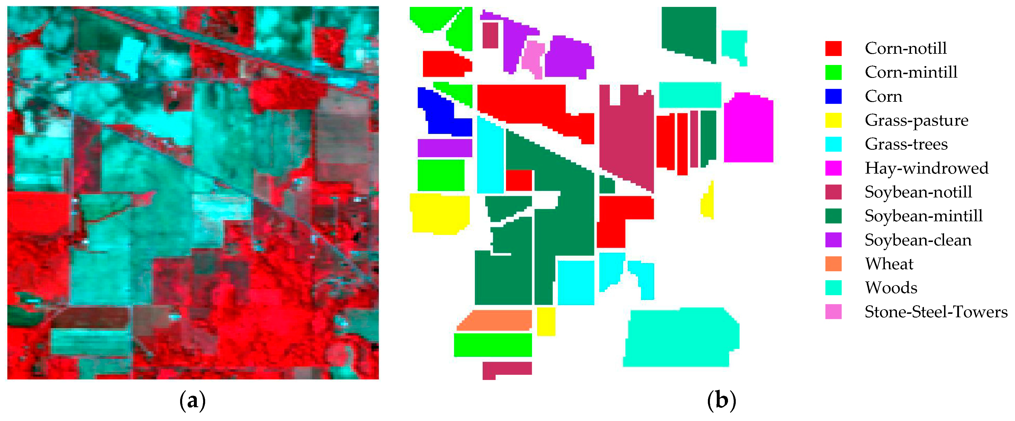
The third dataset used in the experiments was collected by the AVIRIS sensor over the Indian Pines Test Site in Northwestern Indiana in 1992. This image has a size of 145 × 145 pixels, and was acquired over a mixed agricultural/forest area, early in the growing season. The spatial resolution is approximately 20 m, and the radiometric resolution is 10 bits. The image comprised 220 spectral channels in the wavelength range from 0.4–2.5 micrometers, nominal spectral resolution of 10 nanometers. Bands 1–2, 100–114, 147–167, and 216–220 were removed from the dataset due to the noise and the water absorption phenomena, leaving a total of 177 radiance channels to be used in the experiments. This scene contained two-thirds agriculture and one-third forest or other natural perennial vegetation. For illustrative purposes, Figure 11a shows a false color composition of the AVIRIS Indian Pines scene, while Figure 11b shows the ground truth map available for the scene, with 16 classes. In our experiments, we considered a real situation in which most of the similar classes were included in the evaluations. Hence, 12 classes with an adequate number of labeled samples were selected for the experiments.
4.2. Experiments on the Simulated Dataset
The proposed ISI-PS algorithm was firstly performed on the simulated dataset, which was generated using the elements of Table 1. This data contained five datasets with different numbers and types of endmembers. In order to generate the fractional abundance for each dataset, a different pattern was employed according to Table 1. The main objective of this experiment was to evaluate the performance of the proposed method to deal with the endmembers’ SV and decreasing the correlation of endmembers by selecting the optimal bands to generate accurate fractional abundances. Besides, the quality of endmembers’ sets—which had been extracted in an unsupervised manner according to Figure 1—were compared with a spectral library that existed for the ground truth maps.
Several scenarios have been designed in order to evaluate the performance of the proposed method. In addition to the variety of spectral features and spatial patterns, different signal-to-noise ratios (i.e., 20:1, 25:1, and 30:1) have been employed to generate the simulated images. Equation (5) was used directly to simulate the first four datasets. In the case of the last dataset, in addition to Equation (5), two spectra from different species of one material were used to complicate the SV condition (Figure 12).
As was mentioned in the fifth step of the proposed method, a threshold value (T) was employed to identify the independent bands in the PS. In other words, if the angle of the candidate band from all previously selected bands was greater than the threshold value, this band had a distinct behavior dealing with other selected bands.
The value of this threshold (T) was affected by the number, spectral similarity, and variety of endmembers in the scene. However, if a precise ground truth map were available, the root mean square error (RMSE) resulted from the comparison of this map, and the estimated fractional abundance could be used to properly evaluate this threshold value. In this regard, by increasing the threshold value in the range of 0.5–5 degrees with an increment of 0.25 degrees and evaluating the precision of the resulted fractional abundances, the threshold that led to the minimum error was selected. The results of different scenarios are provided in Table 2, along with the number of selected bands in each method.
If there were no in situ information for establishing a spectral library of the endmembers’ variability, this information could be directly extracted from the image according to the early stages of the proposed algorithm. In this process—which was developed by applying some revisions to the SSPP algorithm—the virtual dimensionality (VD) of data was firstly estimated using the signal subspace identification algorithms (e.g., Hysime [28]) to be used for spectral dimension reduction by employing PCA or MNF transformations. Thereafter, the data used were also reduced in the spatial domain using spectral purity indices such as the PPI, and consequently, the number of candidate pure pixels was decreased. Using the mean spectrum of spectral clusters as the indicator of those classes without eliminating impure pixels led to the mean spectrum being affected by these pixels. In this case, the spectral changes among the clusters’ pixels were not only due to the SV phenomena. By clustering those pixels that were probably pure, besides the tending of the class’ mean towards the purity, the separability of classes would be properly shown.
Some other factors that challenged the performance of endmember extraction algorithms were sensitivity to noise, unusual pixels resulting from inaccurate atmospheric correction, and the image’s hot spots. Therefore, extracting the homogeneous area of the image as a possible location for pure pixels could help to reduce the impact of these annoying phenomena. However, this could destroy the information of anomaly classes.
In order to identify the homogenous regions of the image used, a Gaussian filter with the functional form of was firstly applied to each band of the hyperspectral image (Equation (6)). In this filter, the parameter σ controls the amount of spatial smoothing.
where is the value of the pixel (i,j) in the band b of the filtered image. The value of was determined regarding the filter dimension , and showed the spatial index of the filter. In order to generate the spatial homogeneity index (SHI), the RMSE of the discrepancies of the original image and the filtered imaged was computed using Equation (7) [27].
In this way, a layer was obtained where the value of the pixel (i,j) indicates the homogeneity of that region of the image. The lower the pixel value, the more homogeneous that region will be.
Finally, pixels that were located in each cluster were sorted based on the spectral purity index, and the purest ones that were located in homogenous areas were selected as the indicators of those clusters. In the experiments, 20 percent of the pixels of each cluster and 30 percent of the homogenous pixels with the best scores were employed. The results obtained from the subsections of this process are illustrated in Figure 13 for the first dataset.
The results obtained from the SU of the five simulated datasets are provided in Table 3. It is worth mentioning that the endmembers’ sets were directly extracted from the image in these experiments. For comparison purposes, the data used in these experiments were quite similar to those that were used in the previous supervised experiments.
According to Table 2 and Table 3, the proposed ISI-PS algorithm always provided proper accuracy in the estimation of fractional abundances of endmembers by selecting the optimal bands. Moreover, the results obtained from the supervised and unsupervised experiments had good agreement with each other. Therefore, the spectral library of endmembers’ variability was correctly extracted. The accuracies of the fractional abundances obtained from the MTD and ISI-PS methods were compatible. However, by comparing the position of selected bands in these two methods, it is obvious that in the MTD algorithm, the SV of endmembers was neglected, and the most separable bands were selected only by considering the spectral feature of each class. When the SV of the endmembers’ sets was not to the extent that the spectrum of classes highly conflicted in the overlapping regions, the results of the two methods were close to each other. However, if the SV disrupted the separability of classes, the proposed ISI-PS method led to more accurate results by selecting the bands with the minimum spectral conflicts.
4.3. Experiments on Real Datasets
In order to evaluate the effect of SV on the results of unmixing, the ground truth map of the data used was needed, as well as the spectral library of the intra-class variations of each endmember. Providing the sub-pixel fractional abundance of the image’s components was practically impossible, and collecting a spectral library from the variation of each component was an expensive and time-consuming process. However, in the case of the LTRAS dataset, for which only one crop was planted in each farm, the fraction of the components could be supposed to be 100 percent in the related plot; and observed spectral variations among the pixels of each plot could be seen as their SV due to the factors mentioned in Section 4.1.2.
However, it is worth mentioning that the change of the ratio of plants and background soil in each farm will lead to the change of the received spectra. This type of change was not considered as spectral variability. In this study, regarding the rather limited area and homogeneity of the farms, it was assumed that the mixture of materials was accrued with a constant ratio.
The extraction of the statistics of each class was performed using five percent of its pixels, which were selected randomly. This subset was used as the training dataset, and the remaining part was employed as the test dataset. Regarding the intra-class variations, the spectral features of the training pixels were employed for establishing a spectral library for each class. The mean spectrum of these sets was then used as the spectral indicator of the related classes.
As previously mentioned, the correlation of bands was not considered in the prioritization process of the SZU method. The selected bands using this method are illustrated by green bars in Figure 14. As can be seen, several bands were selected in the vicinity of each other in the event that the behavior of the endmembers was close together in these bands. In other words, if this redundancy could be reduced by a meaningful selection of the optimal bands in each region, more accurate and computationally-effective results could be achieved.
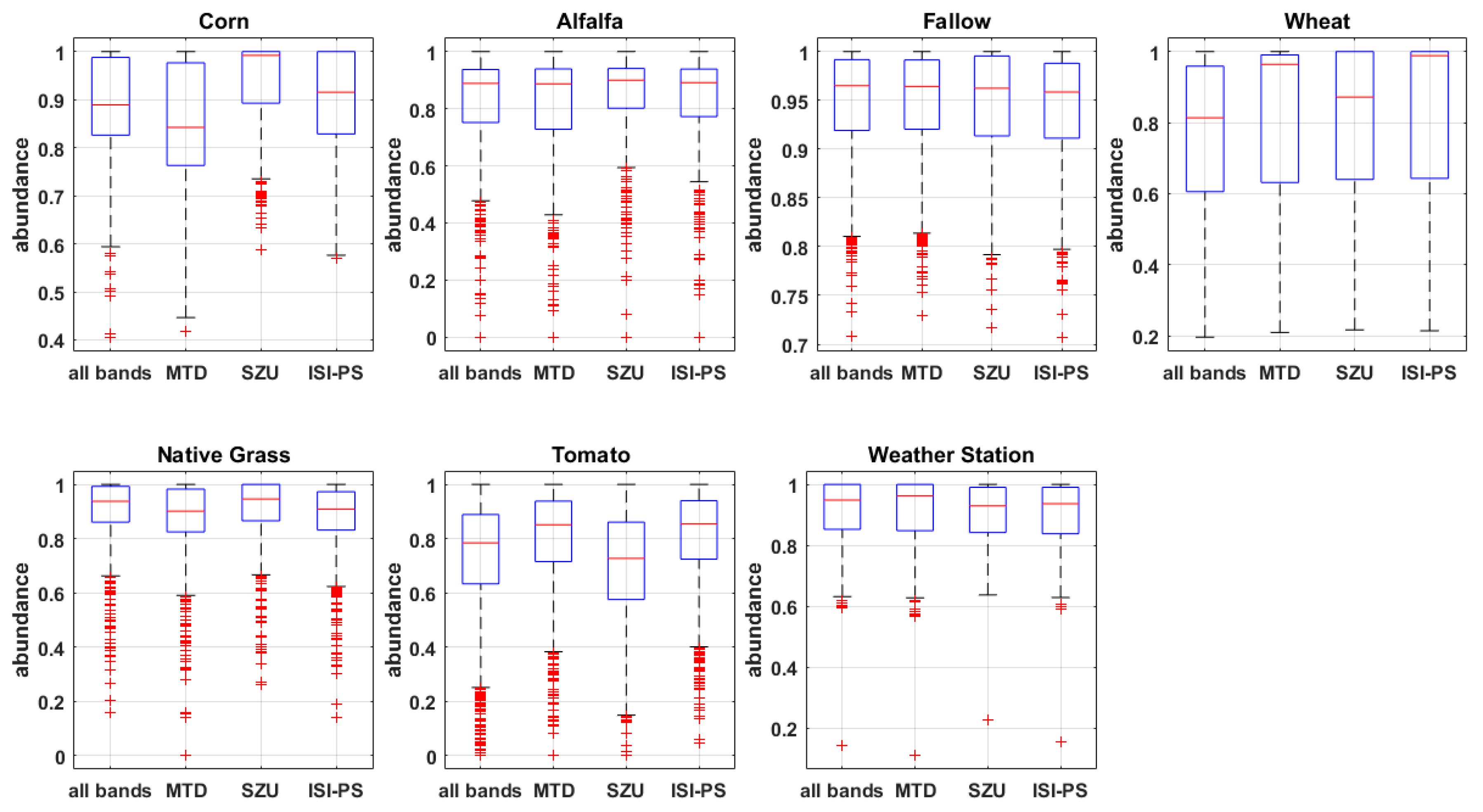
In the proposed ISI-PS algorithm, the angle of bands was used in the PS to deal with the bands’ correlation. The selection of a proper threshold (T) to eliminate the correlated bands was affected by the number, spectral similarity, and variety of endmembers in the scene, as well as the number of resulting bands. If a ground truth map were available, the proper angle to eliminate the redundant bands could be estimated using the estimation accuracy of the ground truth map. In this experiment, regarding the homogeneity of farms, a ground truth map was generated using the map shown in Figure 6b. In this regard, the fraction of each endmember in the related class was considered as one, and for other classes, the fractions were considered to be zero. The fraction of classes in each pixel was then estimated involving the selected bands in each method, and their box plots are illustrated in Figure 15. In this case, the closer the resulting fraction to one and the less the standard deviation of fractions, the better the performance of the algorithm for dealing with the intra-class variations. It is worth mentioning that the most SV had occurred in the corn, wheat, and tomato classes. As can be seen, in comparison with the MTD method, the proposed ISI-PS algorithm tried to reduce the SV in these classes by decreasing the median and the standard deviation of the estimated fractions. However, in the other classes, the performances of the studied methods were close to each other.
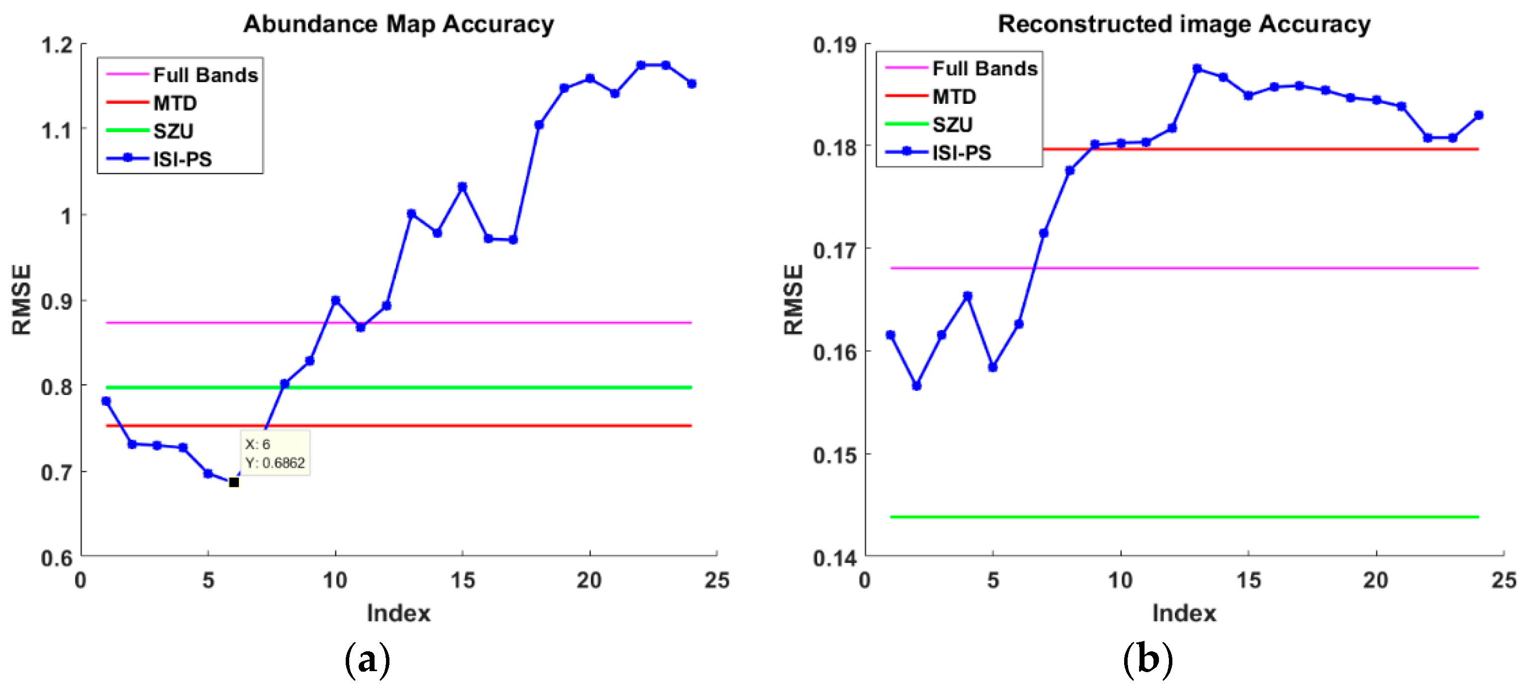
In this experiment, the threshold value of the correlated bands was considered as 1.25 degrees. Figure 16a shows the RMSE of the fractional abundance estimation of the LTRAS classes using the bands obtained from the MTD, the SZU, and the proposed ISI-PS algorithms, for threshold values of 0.25–5 degrees by an increment of 0.2 degrees. Index 6 was equivalent to the threshold value of 1.25 degrees, and caused the selection of 46 bands from the original 170 bands. The selected bands using the MTD, the SZU, and the ISI-PS algorithms are illustrated in Figure 14 using red, green, and dashed blue lines, respectively. It is worth mentioning that the proposed ISI-PS algorithm provided the most accurate fractions.
The singularity of the coefficient matrix, which was generated using the selected bands, was evaluated using: (1) the condition number of the endmembers matrix and (2) the average correlation of the endmembers’ correlation matrix. By increasing the number of selected bands using each method, these two measures are illustrated in Figure 17, as well as for the full dimension of the data (i.e., all bands).
Finally, to evaluate the role of the selected bands on the results, the original image was reconstructed using the same set of endmembers and fractional abundances obtained from each method. In other words, by considering the accuracy of endmembers and applying the LMM, each pixel (y) of the original image could be approximated using , where p is the number of endmembers, is the estimated fractions for each endmember, and is the ith endmember. Accordingly, the original and the reconstructed images using the LMM could be considered as and , respectively, where N is the number of pixels. The reconstruction accuracy could be estimated using Equation (8). The average reconstruction error of each method is illustrated in Figure 16b, and the obtained results from the SU process are provided in Table 4.
In the unsupervised manner, the dimension of the signal subspace was firstly estimated as nine using the HySime algorithm. Then, according to the proposed method, a spectral library was established from the spectral variability of each class, regardless of the ground truth map. In order to evaluate the spectral similarity of the endmembers obtained with the spectrum of each class from the ground truth map, the average spectra of the two sets was compared with the spectral information divergence (SID) [39] similarity measure. The results obtained are provided in Table 5. The lower the value of SID, the more similar the two spectra will be. According to the results, the corn class was split into three sub-classes. However, the spectrum of the other classes was estimated properly.
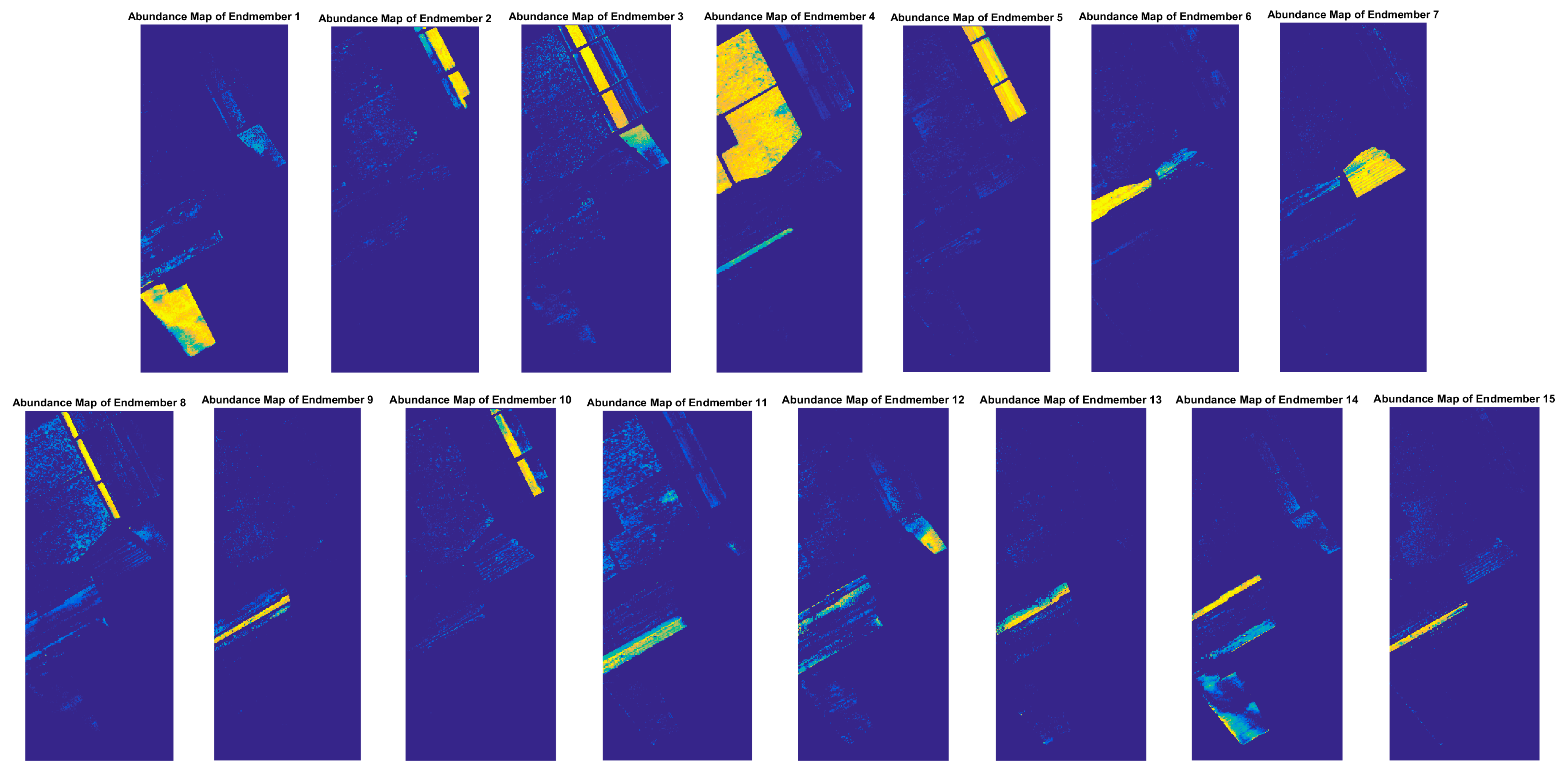
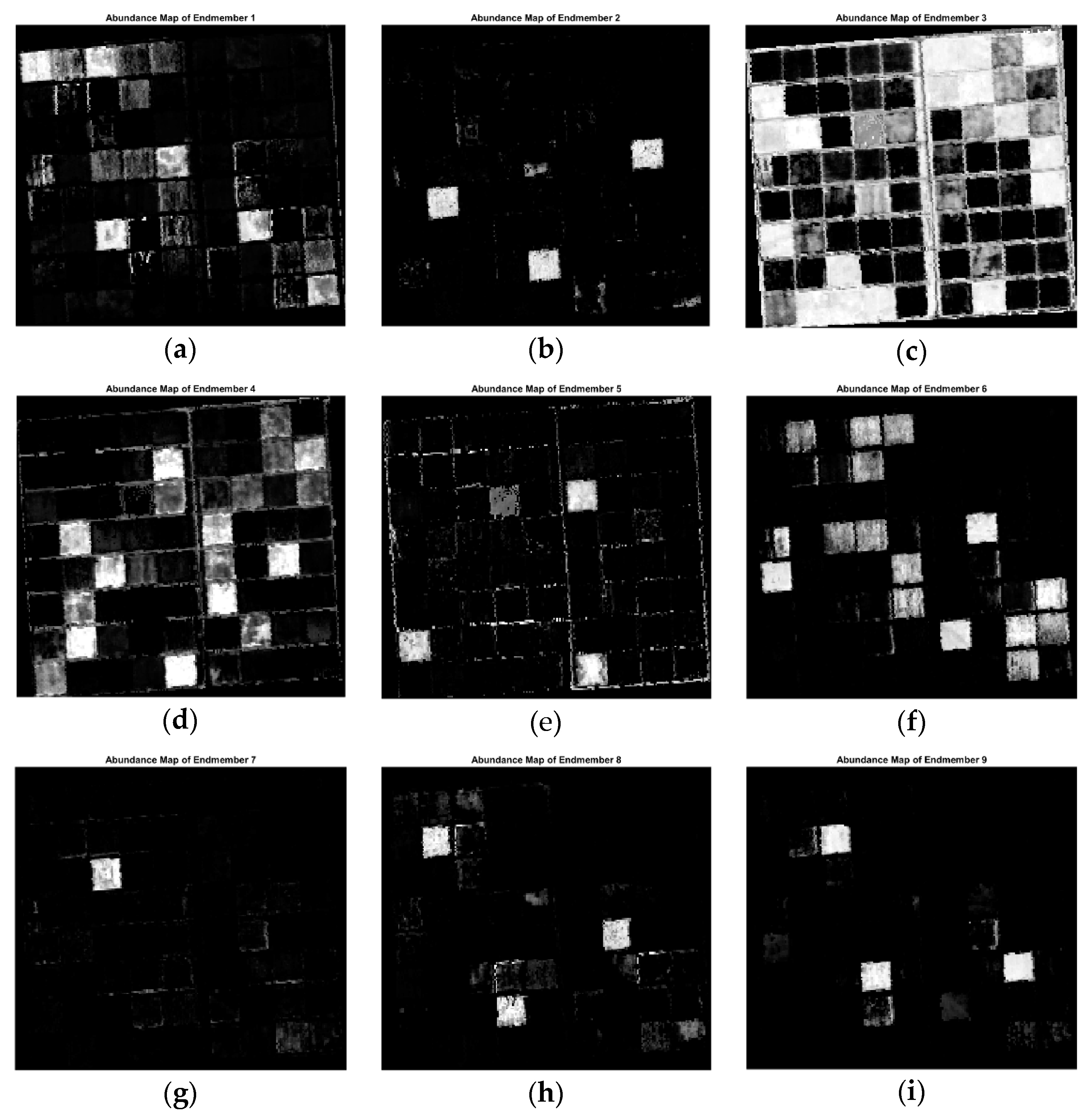
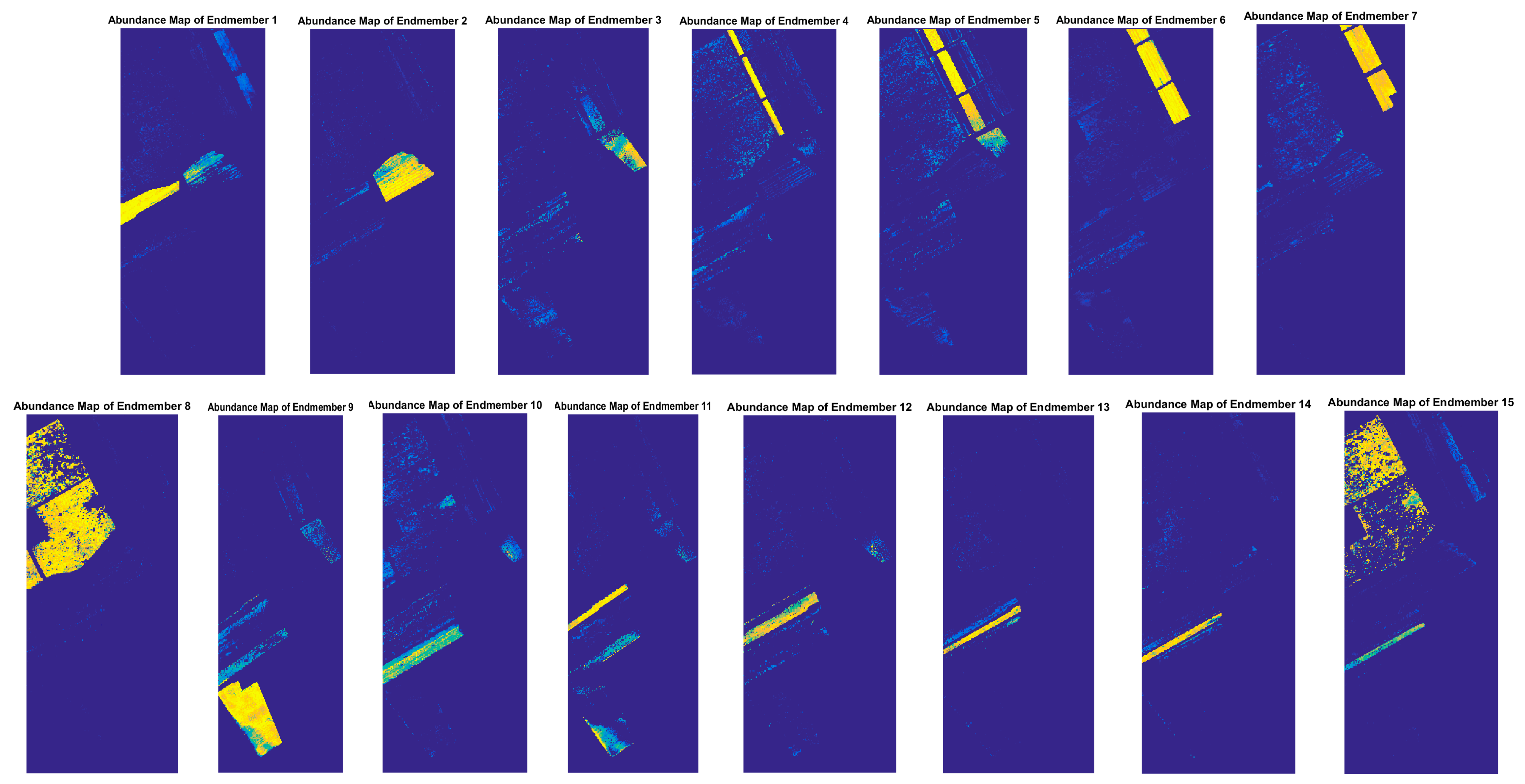
The estimated fractional abundances using the 61 selected bands by the proposed ISI-PS algorithm (Table 4) and the FCLS method are illustrated in Figure 18. As can been seen, the corn class was split into three sub-classes, as in Figure 18a,h,i. The fractional abundances of the bare soil and the wheat classes (i.e., Figure 18c,d, respectively) were partially overlaid, which was due the harvesting of wheat and the appearance of the background soil of the farms. It is worth mentioning that this issue had mostly occurred in farms with a lesser vegetation density due to the type of irrigation and fertilization. This could be obviously understood by the comparison of the obtained results and Figure 7.
All of the pre-mentioned process for the LTRAS dataset was performed on the Salinas and Indiana Indian Pines datasets as well (Table 4).
In this table, in order to evaluate the accuracy of the proposed method when no in situ data were available, the results have been provided for the supervised and the unsupervised manners. In the unsupervised approach, the endmember sets were extracted from the image without any prior knowledge. In this regard, using the position of the pure pixels obtained, a fractional map with a 100 percent abundance was first generated for each endmember to compute the threshold value. Then, the fractional abundances of the endmembers were estimated using the extracted endmembers and the different bands obtained from different threshold values. Finally, the threshold value that led to the minimum RMSE of the estimation of the fractional abundances of endmembers was selected as the optimal threshold value.
In order to compare the results obtained from the supervised and the unsupervised approaches, the estimated fractional maps using the FCLS method over the Salinas dataset are illustrated in Figure 19 and Figure 20. As can be seen, the results of the unsupervised approach were compatible with the supervised approach, and the proposed method was able to separate the similar spectral classes. However, due to the similar spectral behaviors in the endmember extraction step, the two classes grapes_untrained and vineyard_untrained were considered as unique classes.
In this section, a comparison is made between the computational times of different methods and is reported in Table 6. All of the methods were executed on a PC with an i7 5820k CPU and 32 GB of RAM.
As can be seen, ISI-PS showed disadvantages from the computational time point of view. This was mainly due to the exhaustive search, which was applied to locate an optimum value for threshold T (see Section 3.4). We had chosen a rather vast domain of T for the sake of a richer evaluation. However, the processing time of ISI-PS can be highly improved by a more exact estimation of the search domain for T. In addition, more advanced search strategies—instead of the exhaustive search applied herein—can be of great help to mitigate the computational costs of ISI-PS, which is suggested for further study.
5. Conclusions
Band selection has been always a challenge in the processing of high-dimensional hyperspectral data. In this paper, a novel method was presented to select a subset of bands that led especially to improving the results of spectral unmixing. The proposed method—named ISI-PS—integrates two measures of band selection. Firstly, it is aimed at managing the spectral variability. To do so, the bands were prioritized in a way so as to have the least inter-class variability while at the same time achieving the highest possible between-class separation. On the other hand, the second phase takes into account the bands’ dependency and makes an effort to detect and remove highly correlated bands. This phase was performed in the Prototype Space, which was formed by image endmembers. In the Prototype Space—in which the bands were treated as the space points—bands’ dependencies were examined via their inter-angles.
As mentioned above, the second phase of the proposed method required the knowledge of image endmembers, which is itself a challenge in hyperspectral image processing. In this paper, as with the other contribution, an unsupervised automatic technique was proposed that can effectively extract the endmembers from the image itself and that needed no more input knowledge.
The proposed method was examined and validated on a variety of simulated and real datasets. To do so, the selected bands were used in the spectral unmixing, and the RMSE of the obtained fractional abundances was considered as the accuracy measure. The obtained results were all compatible with the in-situ observations and confirmed the effectiveness of the proposed method. In addition, the performance of the proposed method was compared with the SZU and the MTD algorithms, which proved the superiority of the proposed method.
Author Contributions
All of the authors listed contributed equally to the work presented in this paper.
Conflicts of Interest
The authors declare no conflict of interest.
References
- Li, C.; Ma, Y.; Mei, X.; Liu, C.; Ma, J. Hyperspectral unmixing with robust collaborative sparse regression. Remote Sens. 2016, 8, 588. [Google Scholar] [CrossRef]
- Liu, R.; Du, B.; Zhang, L. Hyperspectral unmixing via double abundance characteristics constraints based nmf. Remote Sens. 2016, 8, 464. [Google Scholar] [CrossRef]
- Bioucas-Dias, J.M.; Plaza, A.; Dobigeon, N.; Parente, M.; Du, Q.; Gader, P.; Chanussot, J. Hyperspectral unmixing overview: Geometrical, statistical, and sparse regression-based approaches. IEEE J. Sel. Top. Appl. Earth Obs. Remote Sens. 2012, 5, 354–379. [Google Scholar] [CrossRef]
- Somers, B.; Asner, G.P.; Tits, L.; Coppin, P. Endmember variability in spectral mixture analysis: A review. Remote Sens. Environ. 2011, 115, 1603–1616. [Google Scholar] [CrossRef]
- Xu, M.; Zhang, L.; Du, B.; Zhang, L.; Fan, Y.; Song, D. A mutation operator accelerated quantum-behaved particle swarm optimization algorithm for hyperspectral endmember extraction. Remote Sens. 2017, 9, 197. [Google Scholar] [CrossRef]
- Settle, J. On the effect of variable endmember spectra in the linear mixture model. IEEE Trans. Geosci. Remote Sens. 2006, 44, 389–396. [Google Scholar] [CrossRef]
- Iordache, M.D.; Bioucas-Dias, J.M.; Plaza, A. Sparse unmixing of hyperspectral data. IEEE Trans. Geosci. Remote Sens. 2011, 49, 2014–2039. [Google Scholar] [CrossRef]
- Van der Meer, F.D.; Jia, X. Collinearity and orthogonality of endmembers in linear spectral unmixing. Int. J. Appl. Earth Obs. Geoinf. 2012, 18, 491–503. [Google Scholar] [CrossRef]
- Mojaradi, B.; Abrishami-Moghaddam, H.; Zoej, M.J.V.; Duin, R.P.W. Dimensionality reduction of hyperspectral data via spectral feature extraction. IEEE Trans. Geosci. Remote Sens. 2009, 47, 2091–2105. [Google Scholar] [CrossRef]
- Zare, A.; Ho, K. Endmember variability in hyperspectral analysis: Addressing spectral variability during spectral unmixing. IEEE Signal Proc. Mag. 2014, 31, 95–104. [Google Scholar] [CrossRef]
- Xu, X.; Tong, X.; Plaza, A.; Zhong, Y.; Xie, H.; Zhang, L. Joint sparse sub-pixel mapping model with endmember variability for remotely sensed imagery. Remote Sens. 2016, 9, 15. [Google Scholar] [CrossRef]
- Asner, G.P.; Lobell, D.B. A biogeophysical approach for automated swir unmixing of soils and vegetation. Remote Sens. Environ. 2000, 74, 99–112. [Google Scholar] [CrossRef]
- Somers, B.; Delalieux, S.; Verstraeten, W.; Van Aardt, J.; Albrigo, G.; Coppin, P. An automated waveband selection technique for optimized hyperspectral mixture analysis. Int. J. Remote Sens. 2010, 31, 5549–5568. [Google Scholar] [CrossRef]
- Richards, J.A. Remote Sensing Digital Image Analysis: An Introduction; Springer: Berlin, Germany, 2012. [Google Scholar]
- Green, A.A.; Berman, M.; Switzer, P.; Craig, M.D. A transformation for ordering multispectral data in terms of image quality with implications for noise removal. IEEE Trans. Geosci. Remote Sens. 1988, 26, 65–74. [Google Scholar] [CrossRef]
- Wang, L.; Jia, X.; Zhang, Y. A novel geometry-based feature-selection technique for hyperspectral imagery. IEEE Geosci. Remote Sens. Lett. 2007, 4, 171–175. [Google Scholar] [CrossRef]
- Du, Q.; Yang, H. Similarity-based unsupervised band selection for hyperspectral image analysis. IEEE Geosci. Remote Sens. Lett. 2008, 5, 564–568. [Google Scholar] [CrossRef]
- Asl, M.G.; Mobasheri, M.R.; Mojaradi, B. Unsupervised feature selection using geometrical measures in prototype space for hyperspectral imagery. IEEE Trans. Geosci. Remote Sens. 2014, 52, 3774–3787. [Google Scholar]
- Somers, B.; Zortea, M.; Plaza, A.; Asner, G.P. Automated extraction of image-based endmember bundles for improved spectral unmixing. IEEE J. Sel. Top. Appl. Earth Obs. Remote Sens. 2012, 5, 396–408. [Google Scholar] [CrossRef]
- Winter, M.E. N-findr: An Algorithm for Fast Autonomous Spectral End-Member Determination in Hyperspectral Data. In Proceedings of the SPIE’s International Symposium on Optical Science, Engineering, and Instrumentation, Denver, CO, USA, 27 October 1999. [Google Scholar]
- Harsanyi, J.C.; Chang, C.-I. Hyperspectral image classification and dimensionality reduction: An orthogonal subspace projection approach. IEEE Trans. Geosci. Remote Sens. 1994, 32, 779–785. [Google Scholar] [CrossRef]
- Chang, C.I. Hyperspectral Imaging: Techniques for Spectral Detection and Classification; Springer: New York, NY, USA, 2003; Volume 1. [Google Scholar]
- Neville, R.; Staenz, K.; Szeredi, T.; Lefebvre, J.; Hauff, P. Automatic Endmember Extraction from Hyperspectral Data for Mineral Exploration. In Proceedings of the 21st Canadian Symposium on Remote Sens, Ottawa, ON, Canada, 21–24 June 1999. [Google Scholar]
- Nascimento, J.M.P.; Dias, J.M.B. Vertex component analysis: A fast algorithm to unmix hyperspectral data. IEEE Trans. Geosci. Remote Sens. 2005, 43, 898–910. [Google Scholar] [CrossRef]
- Chang, C.-I.; Chen, S.-Y.; Li, H.-C.; Chen, H.-M.; Wen, C.-H. Comparative study and analysis among atgp, vca, and sga for finding endmembers in hyperspectral imagery. IEEE J. Sel. Top. Appl. Earth Obs. Remote Sens. 2016, 9, 4280–4306. [Google Scholar] [CrossRef]
- Chang, C.I.; Wu, C.C.; Liu, W.; Ouyang, Y.C. A new growing method for simplex-based endmember extraction algorithm. IEEE Trans. Geosci. Remote Sens. 2006, 44, 2804–2819. [Google Scholar] [CrossRef]
- Martin, G.; Plaza, A. Spatial-spectral preprocessing prior to endmember identification and unmixing of remotely sensed hyperspectral data. IEEE J. Sel. Top. Appl. Earth Obs. Remote Sens. 2012, 5, 380–395. [Google Scholar] [CrossRef]
- Bioucas-Dias, J.M.; Nascimento, J.M. Hyperspectral subspace identification. IEEE Trans. Geosci. Remote Sens. 2008, 46, 2435–2445. [Google Scholar] [CrossRef]
- Boardman, J.W.; Kruse, F.A.; Green, R.O. Mapping Target Signatures via Partial Unmixing of Aviris dData. In Proceedings of the Fifth Annual JPL Airborne Earth Science Workshop, Pasadena, CA, USA, 23–26 January 1995. [Google Scholar]
- Rodriguez, A.; Laio, A. Clustering by fast search and find of density peaks. Science 2014, 344, 1492–1496. [Google Scholar] [CrossRef] [PubMed]
- Chang, C.-I.; Wang, S. Constrained band selection for hyperspectral imagery. IEEE Trans. Geosci. Remote Sens. 2006, 44, 1575–1585. [Google Scholar] [CrossRef]
- Chang, C.-I.; Du, Q.; Sun, T.-L.; Althouse, M.L. A joint band prioritization and band-decorrelation approach to band selection for hyperspectral image classification. IEEE Trans. Geosci. Remote Sens. 1999, 37, 2631–2641. [Google Scholar] [CrossRef]
- Heinz, D.C.; Chang, C.-I. Fully constrained least squares linear spectral mixture analysis method for material quantification in hyperspectral imagery. IEEE Trans. Geosci. Remote Sens. 2001, 39, 529–545. [Google Scholar] [CrossRef]
- Hyperspectral Imagery Synthesis Tools for Matlab. Available online: http://www.ehu.es/ccwintco/index.php/Hyperspectral_Imagery_Synthesis_tools_for_MATLAB (accessed on 21 March 2017).
- Nascimento, J.M.P. Unsupervised Hyperspectral Unmixing; Universidade Técnica de Lisboa: Lisbon, Portugal, 2006. [Google Scholar]
- Shaw, G.A.; Burke, H.-H.K. Spectral imaging for remote sensing. Linc. Lab. J. 2003, 14, 3–28. [Google Scholar]
- Russell Ranch Sustainable Agriculture Facility. Available online: http://asi.ucdavis.edu/programs/rr (accessed on 10 March 2017).
- Photos and Maps—Agricultural Sustainability Institute—Uc Davis. Available online: http://asi.ucdavis.edu/programs/rr/photos-and-maps (accessed on 15 March 2017).
- Chang, C.-I. An information-theoretic approach to spectral variability, similarity, and discrimination for hyperspectral image analysis. IEEE Trans. Inf. Theory 2000, 46, 1927–1932. [Google Scholar] [CrossRef]
Figure 1.
Flowchart of the proposed method.

Figure 2.
The spectrum of alunite and kaolinite minerals and the highly-correlated regions among the adjacent bands.
Figure 2.
The spectrum of alunite and kaolinite minerals and the highly-correlated regions among the adjacent bands.

Figure 3.
The Prototype Space (PS) constructed using the two endmembers alunite and kaolinite.

Figure 4.
An example of the fractional abundances that were generated using: (a) Spherical Gaussian fields; (b) Exponential Gaussian fields; (c) Rational Gaussian fields; and (d) Mattern Gaussian fields functions.
Figure 4.
An example of the fractional abundances that were generated using: (a) Spherical Gaussian fields; (b) Exponential Gaussian fields; (c) Rational Gaussian fields; and (d) Mattern Gaussian fields functions.
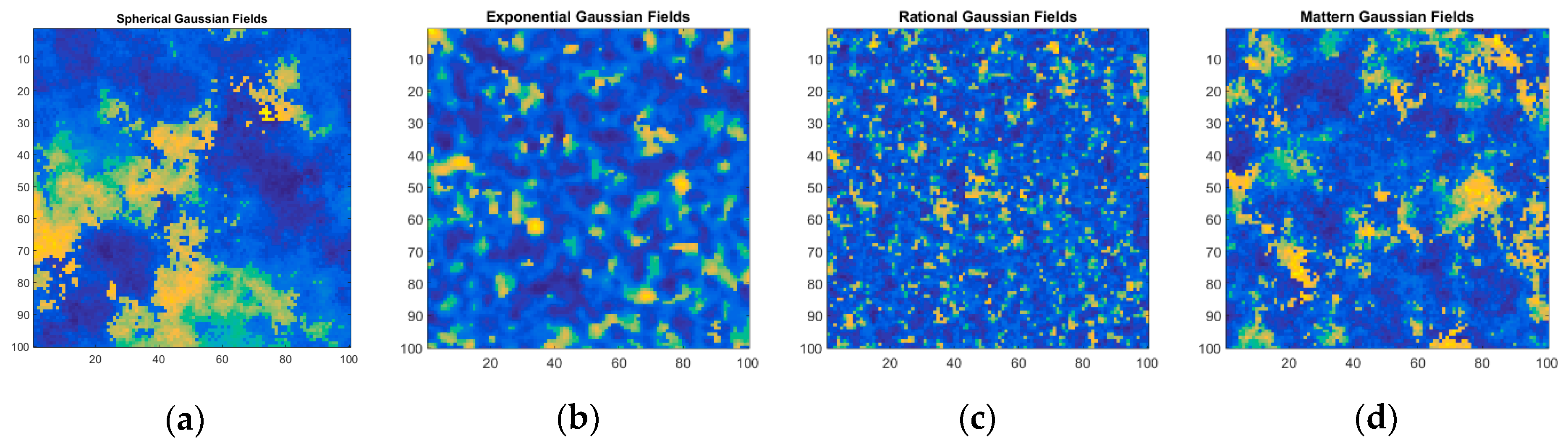
Figure 5.
Flowchart of generating the simulated images.
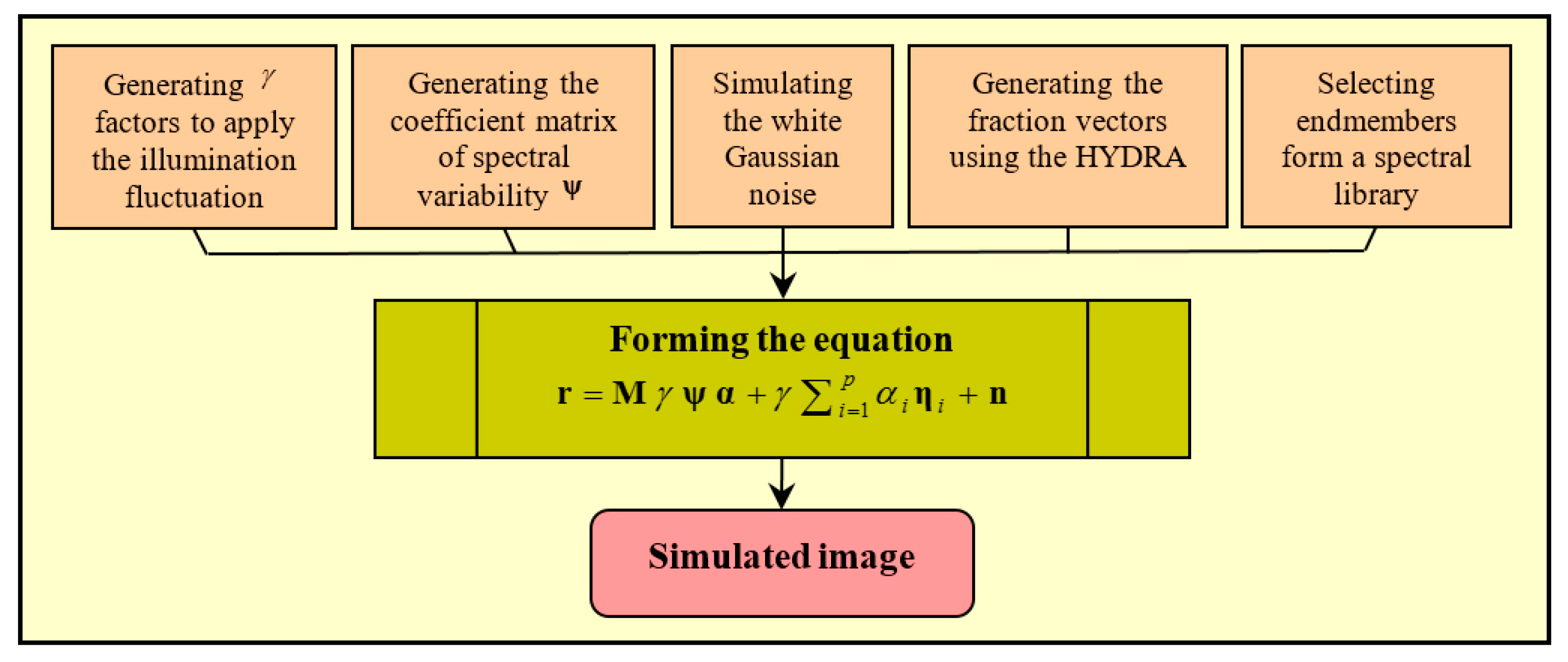
Figure 6.
Long-Term Research in Agricultural Sustainability (LTRAS) dataset: (a) Planting schedule [38]; (b) Ground-truth map of the LTRAS farms.
Figure 6.
Long-Term Research in Agricultural Sustainability (LTRAS) dataset: (a) Planting schedule [38]; (b) Ground-truth map of the LTRAS farms.
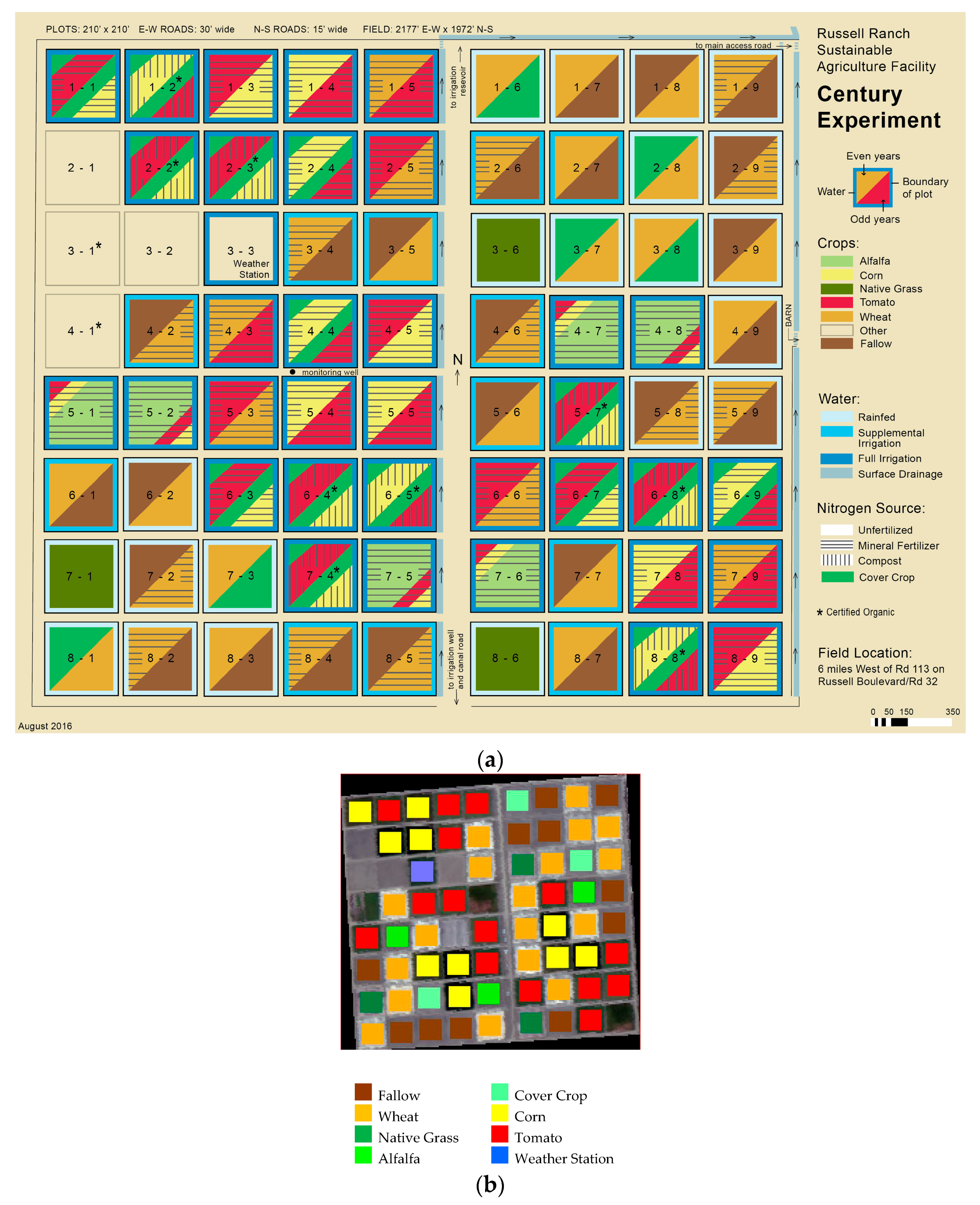
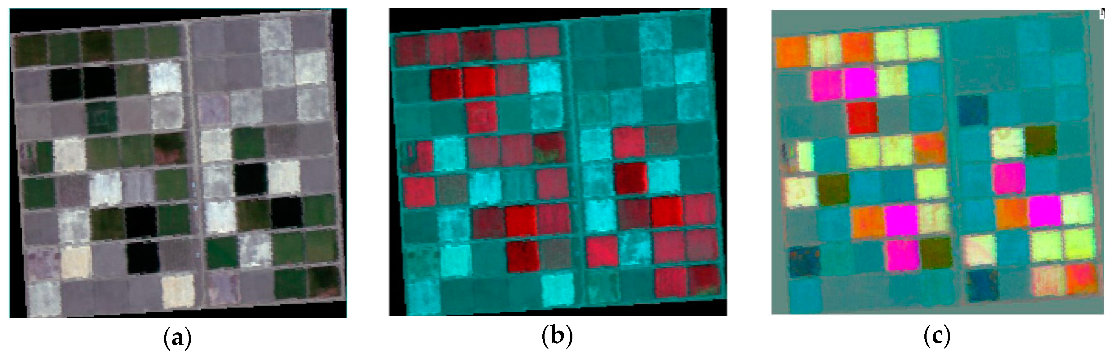
Figure 7.
(a) True color composite; (b) False color composite; and (c) Color composite of the first three components of the maximum noise fraction (MNF) transformation.
Figure 7.
(a) True color composite; (b) False color composite; and (c) Color composite of the first three components of the maximum noise fraction (MNF) transformation.

Figure 8.
The spectral variability of pixels for three classes of: (a) Wheat; (b) Tomato; and (c) Corn.
Figure 8.
The spectral variability of pixels for three classes of: (a) Wheat; (b) Tomato; and (c) Corn.
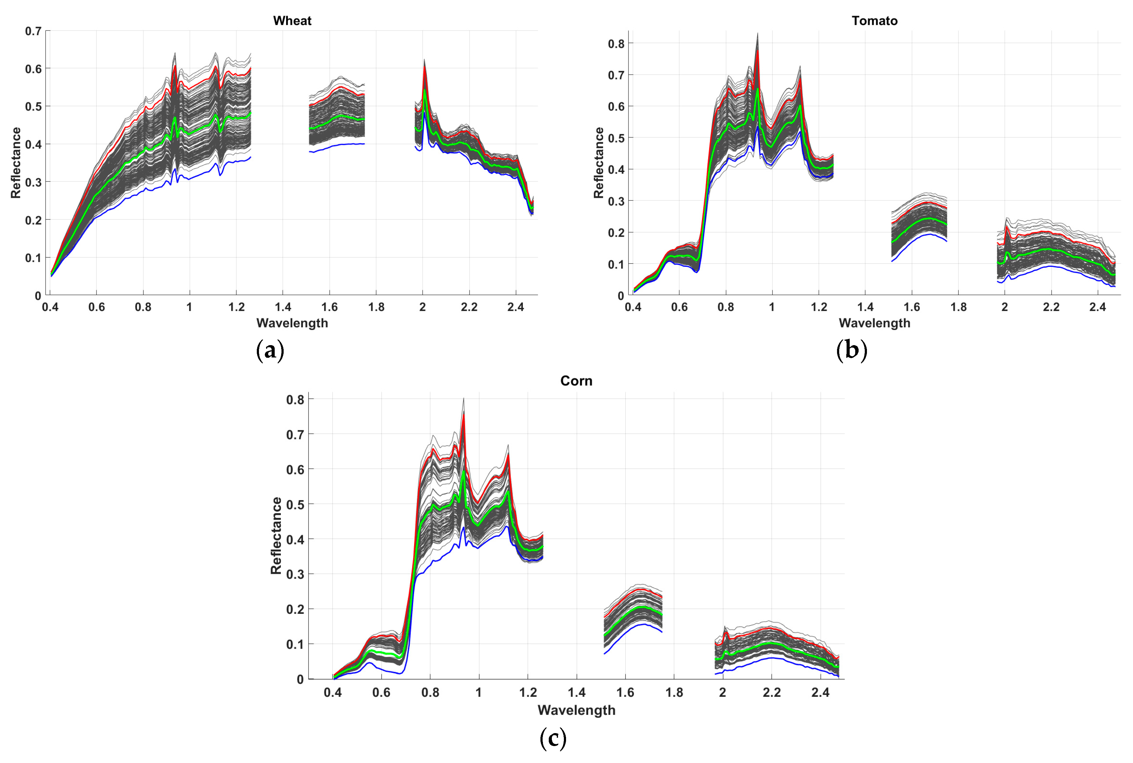
Figure 9.
Salinas dataset: (a) False color composite of the AVIRIS image; (b) Ground truth map.
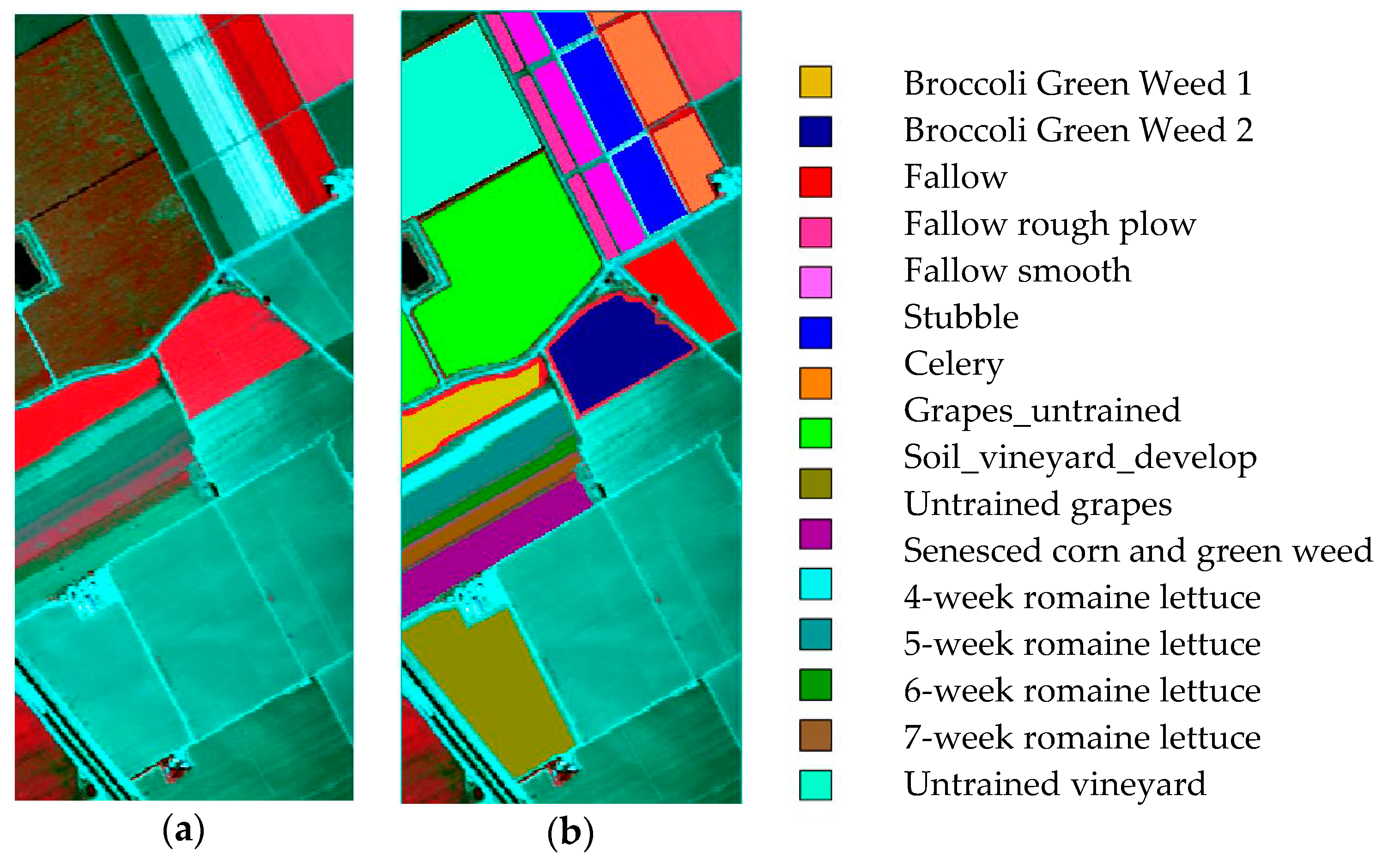
Figure 10.
Photograph of the selected classes in the region of the imaging.
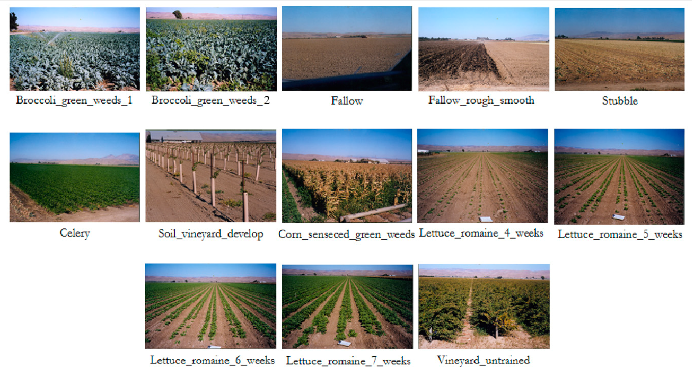
Figure 11.
Indiana Indian Pines dataset: (a) False color composite of the AVIRIS image; (b) Ground truth map.
Figure 11.
Indiana Indian Pines dataset: (a) False color composite of the AVIRIS image; (b) Ground truth map.

Figure 12.
Endmembers used to simulate the last dataset.
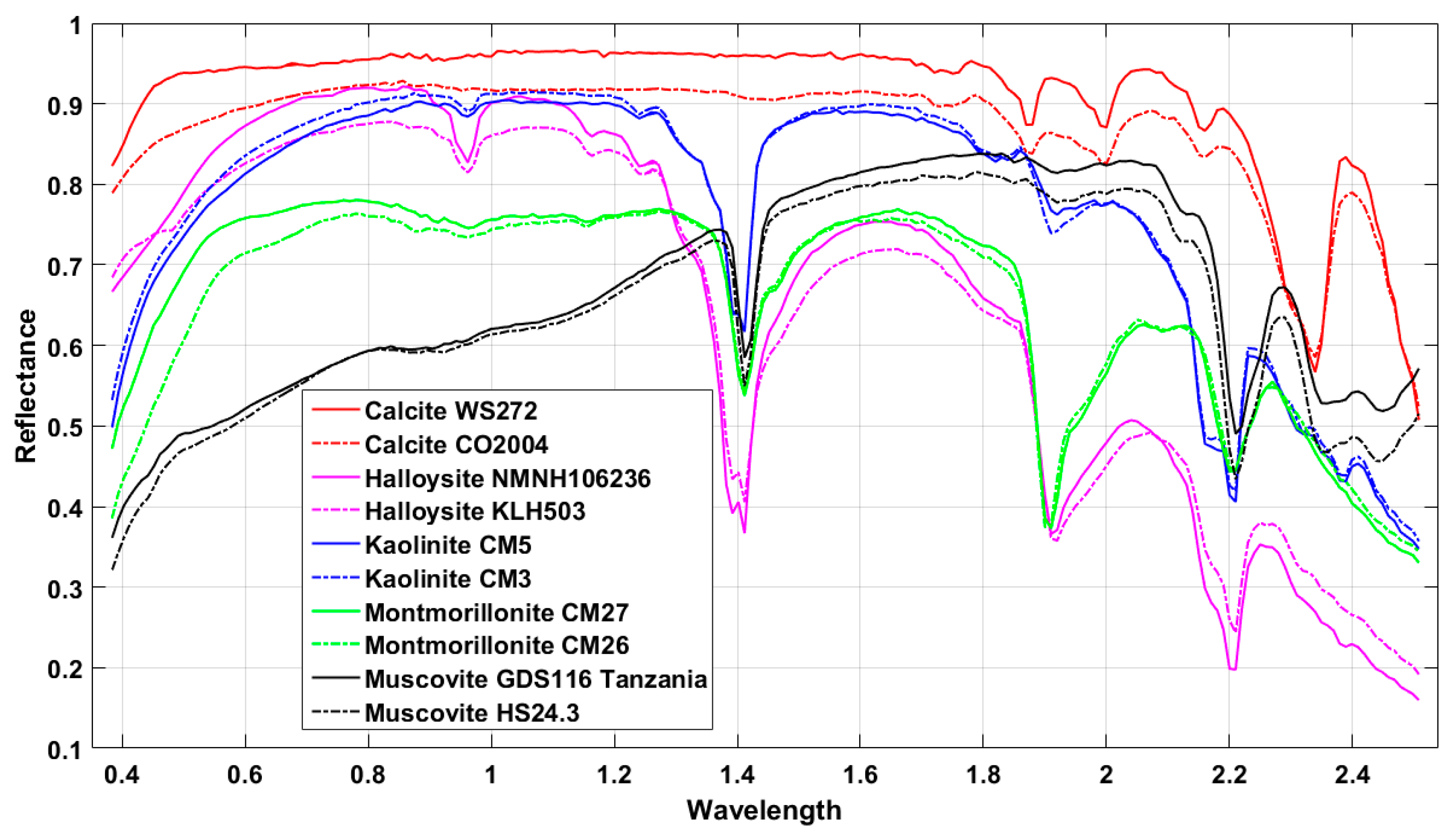
Figure 13.
The results obtained from the subsections of the process of extraction of the spectral library of each class from the image: (a) Output of the pixel purity index (PPI) for greater than zero pixels; (b) The result of band filtering; (c) The clustering of PPI’s output; (d) Map of the homogeneity scores of pixels; (e) 20 percent of pixels of each cluster with the maximum value of PPI; (f) 30 percent of pixels of each cluster with the best homogeneity; (g) Fusion of maps (e,f) to extract the final pure pixels; (h) Ground truth map of the image’s endmembers.
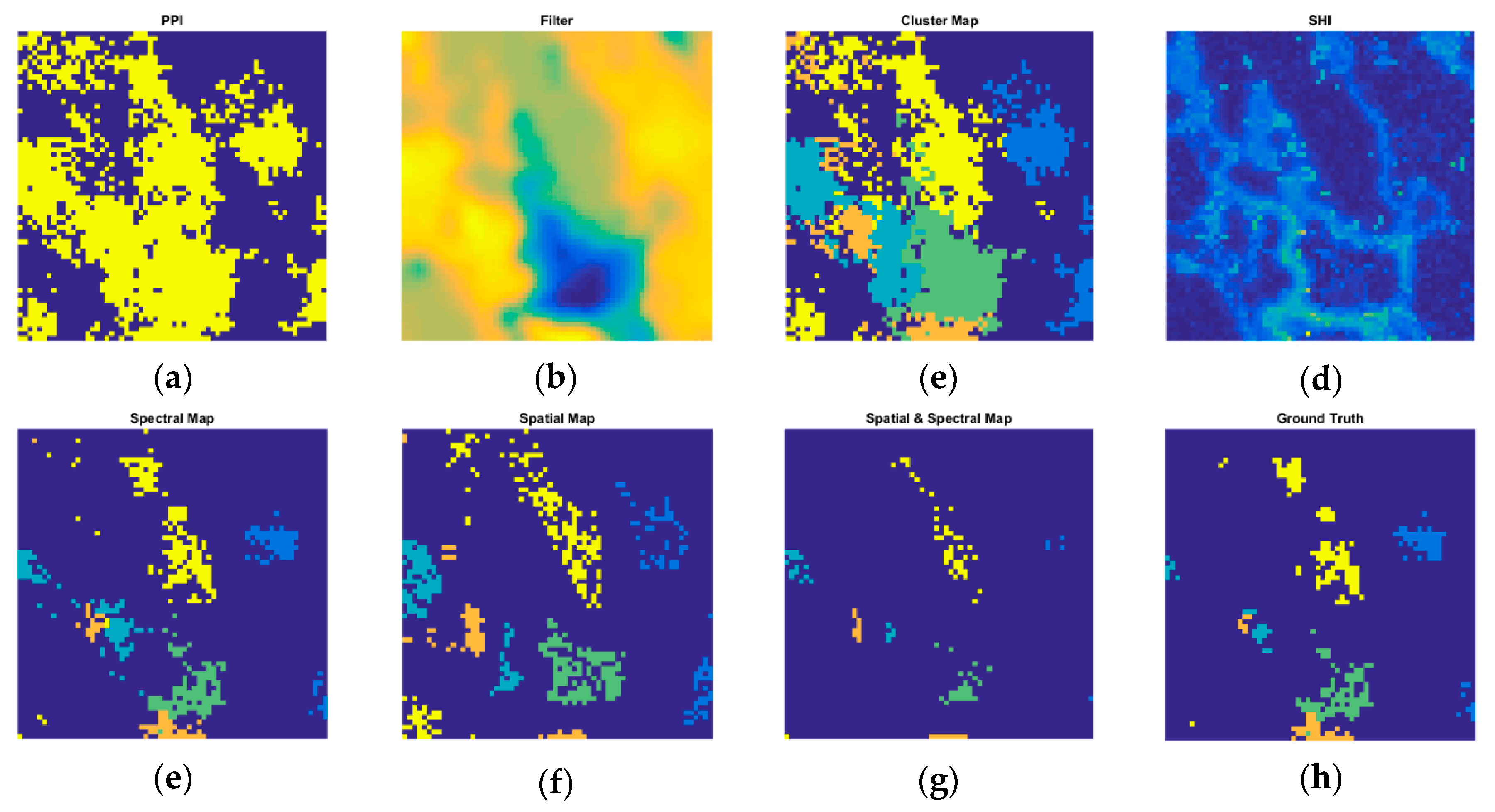
Figure 14.
Representation of the selected bands using the MTD, SZU, and the proposed ISI-PS methods.
Figure 14.
Representation of the selected bands using the MTD, SZU, and the proposed ISI-PS methods.
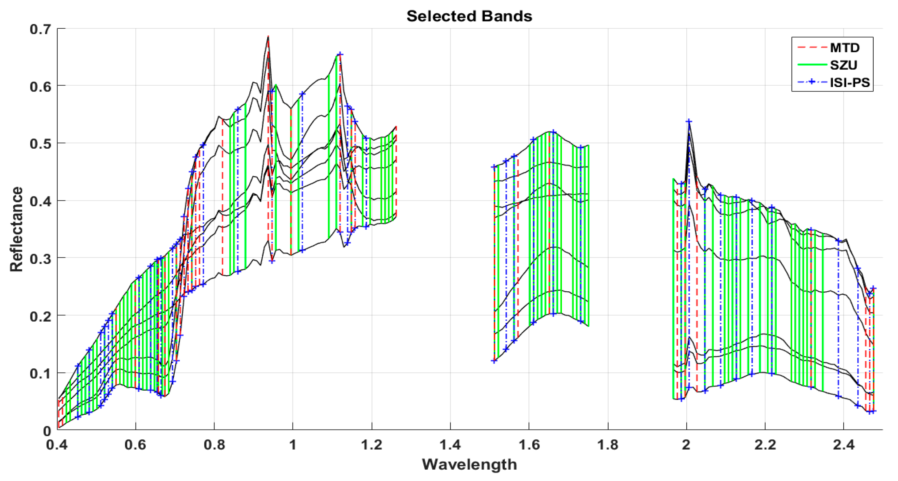
Figure 15.
The box plot of the resulting fractions for each class using the selected bands by the studied method, using: (1) all bands; (2) MTD bands; (3) SZU bands; and (4) ISI-PS bands.
Figure 15.
The box plot of the resulting fractions for each class using the selected bands by the studied method, using: (1) all bands; (2) MTD bands; (3) SZU bands; and (4) ISI-PS bands.

Figure 16.
The RMSE of estimating: (a) The fractions; (b) The LTRAS image by means of the selected bands using the MTD, the SZU, and the ISI-PS algorithms for different threshold values.
Figure 16.
The RMSE of estimating: (a) The fractions; (b) The LTRAS image by means of the selected bands using the MTD, the SZU, and the ISI-PS algorithms for different threshold values.

Figure 17.
Plot of: (a) The condition number of the endmembers matrix; (b) The average correlation of the endmembers’ correlation matrix for the different band selection methods by increasing the number of the selected bands.
Figure 17.
Plot of: (a) The condition number of the endmembers matrix; (b) The average correlation of the endmembers’ correlation matrix for the different band selection methods by increasing the number of the selected bands.
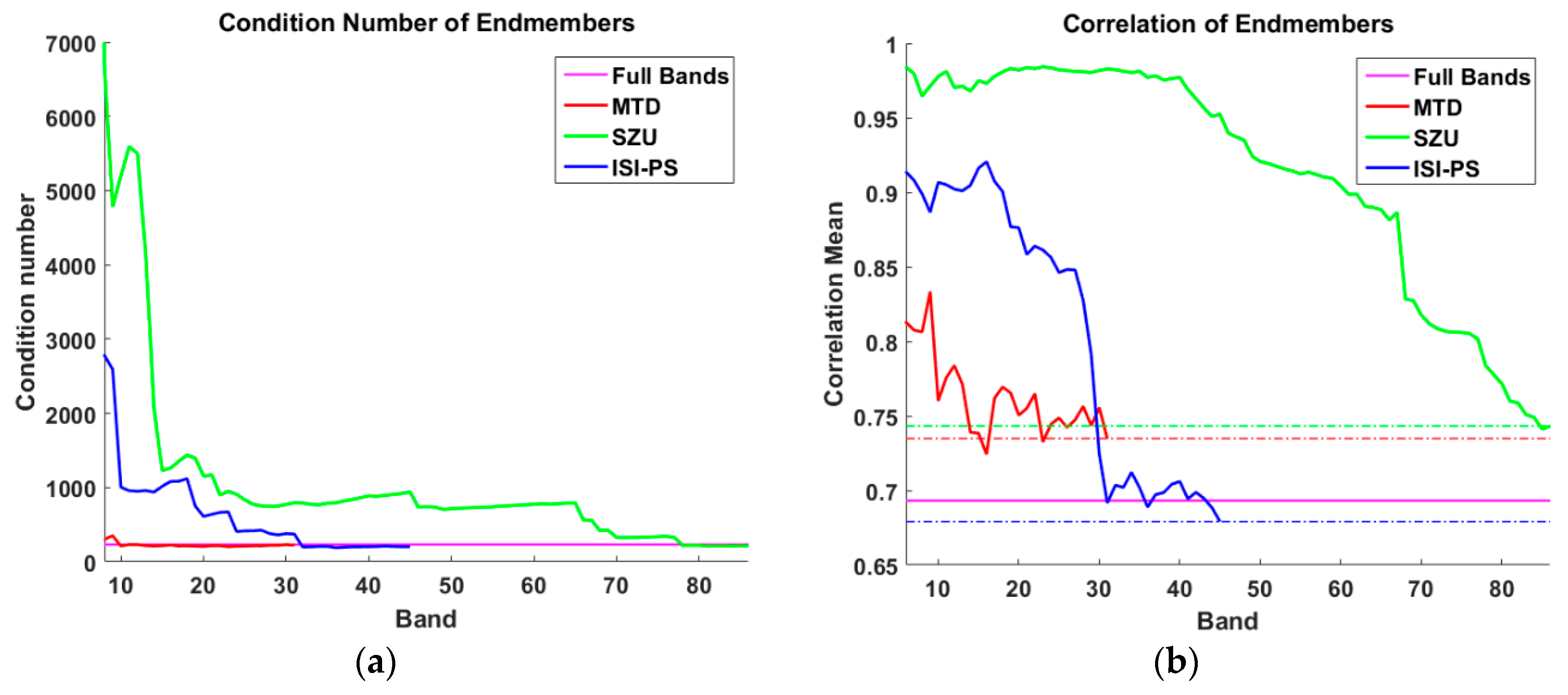
Figure 18.
The estimated fractions using the selected bands by the ISI-PS method in an unsupervised manner for: (a) Corn; (b) Alfalfa; (c) Bare soil; (d) Wheat; (e) Native grass; (f) Tomato; (g) Weather station; (h) Corn; and (i) Corn.
Figure 18.
The estimated fractions using the selected bands by the ISI-PS method in an unsupervised manner for: (a) Corn; (b) Alfalfa; (c) Bare soil; (d) Wheat; (e) Native grass; (f) Tomato; (g) Weather station; (h) Corn; and (i) Corn.

Figure 19.
The fractional abundances estimated from the Salinas area using the fully constrained least squares (FCLS) method and the selected bands by the proposed ISI-PS algorithm in the supervised approach.
Figure 19.
The fractional abundances estimated from the Salinas area using the fully constrained least squares (FCLS) method and the selected bands by the proposed ISI-PS algorithm in the supervised approach.

Figure 20.
The fractional abundances estimated from the Salinas area using the FCLS method and the selected bands by the proposed ISI-PS algorithm in the unsupervised approach.
Figure 20.
The fractional abundances estimated from the Salinas area using the FCLS method and the selected bands by the proposed ISI-PS algorithm in the unsupervised approach.

Table 1.
The constituent spectra of the simulated images.
| Dataset 1 | Dataset 2 | Dataset 3 | Dataset 4 | Dataset 5 | |
|---|---|---|---|---|---|
| Mineral | Alunite HS295.3B Calcite HS48.3B Epidote HS328.3B Kaolinite CM3 Montmorillonite CM20 | Alunite HS295.3B Dickite NMNH106242 Halloysite CM13 Kaolinite CM3 Montmorillonite CM20 | Alunite HS295.3B Halloysite NMNH106 Kaolinite KGa-1 (wxyl) Montmorillonite CM20 Muscovite GDS116 | Alunite HS295.3B Calcite HS48.3B Chlorite HS179.3B Epidote HS328.3B Hematite GDS27 Kaolinite CM3 Montmorillonite CM20 | Calcite WS272, CO2004 Halloysite NMNH106, KLH503 Kaolinite CM5, CM3 Montmorillonite CM27, CM26 Muscovite GDS116, HS24.3 |
| Abundance Map Pattern | Spherical Gaussian Fields | Exponential Gaussian Fields | Rational Gaussian Fields | Mattern Gaussian Fields | Mattern Gaussian Fields |
Table 2.
The accuracy assessment results of the selected bands by maximum tangent discrimination (MTD), stable zone unmixing (SZU), and the proposed instability index (ISI)-prototype space (PS) algorithms, in comparison with using all bands to estimate the fractional abundances through a supervised spectral unmixing on the simulated datasets.
| Data Set | Feature Selection Method | Full Dimensionality | |||||||||||||||||
|---|---|---|---|---|---|---|---|---|---|---|---|---|---|---|---|---|---|---|---|
| ISI-PS | SZU | MTD | |||||||||||||||||
| Abundance Map | #S | SNR | #F | Cond | Corr | RMSE | #F | Cond | Corr | RMSE | #F | T | Cond | Corr | RMSE | #F | Cond | Corr | RMSE |
| Spherical | 5 | 20:1 | 63 | 21.01 | 0.39 | 0.071 | 55 | 28.87 | 0.42 | 0.083 | 29 | 4.00 | 20.97 | 0.40 | 0.071 | 224 | 30.40 | 0.41 | 0.085 |
| Exponential | 5 | 25:1 | 43 | 30.09 | 0.70 | 0.105 | 24 | 117.39 | 0.90 | 0.153 | 27 | 4.00 | 28.99 | 0.68 | 0.103 | 224 | 48.72 | 0.87 | 0.148 |
| Rational | 5 | 30:1 | 68 | 40.98 | 0.51 | 0.090 | 67 | 55.82 | 0.58 | 0.101 | 34 | 3.25 | 36.88 | 0.55 | 0.083 | 224 | 70.58 | 0.53 | 0.112 |
| Mattern | 7 | 25:1 | 61 | 39.54 | 0.19 | 0.063 | 54 | 58.88 | 0.27 | 0.070 | 38 | 3.75 | 38.04 | 0.22 | 0.061 | 224 | 52.50 | 0.21 | 0.068 |
| Mattern | 10 | 30:1 | 65 | 49.71 | 0.58 | 0.181 | 67 | 61.08 | 0.64 | 0.183 | 14 | 4.75 | 34.84 | 0.57 | 0.180 | 224 | 81.72 | 0.61 | 0.187 |
#S is the number the image’s components; #F is the number of selected bands; SNR is the signal-to-noise ratio; Cond is the Condition number; Corr is the mean Correlation of endmembers; T is the angle threshold and bold number is the best result.
Table 3.
The accuracy assessment results of the selected bands by MTD, SZU, and the proposed ISI-PS algorithms, in comparison with using all bands to estimate the fractional abundances through an unsupervised spectral unmixing on to the simulated datasets.
Table 3.
The accuracy assessment results of the selected bands by MTD, SZU, and the proposed ISI-PS algorithms, in comparison with using all bands to estimate the fractional abundances through an unsupervised spectral unmixing on to the simulated datasets.
| Data Set | Feature Selection Method | Full Dimensionality | |||||||||||||||||
|---|---|---|---|---|---|---|---|---|---|---|---|---|---|---|---|---|---|---|---|
| ISI-PS | SZU | MTD | |||||||||||||||||
| Abundance Map | #S | SNR | #F | Cond | Corr | RMSE | #F | Cond | Corr | RMSE | #F | T | Cond | Corr | RMSE | #F | Cond | Corr | RMSE |
| Spherical | 5 | 20:1 | 61 | 20.77 | 0.41 | 0.047 | 138 | 25.81 | 0.42 | 0.050 | 30 | 4.00 | 19.95 | 0.44 | 0.047 | 224 | 32.41 | 0.44 | 0.053 |
| Exponential | 5 | 25:1 | 42 | 28.09 | 0.67 | 0.057 | 124 | 38.88 | 0.82 | 0.062 | 24 | 4.25 | 28.12 | 0.65 | 0.055 | 224 | 45.31 | 0.86 | 0.067 |
| Rational | 5 | 30:1 | 70 | 44.58 | 0.61 | 0.071 | 109 | 62.38 | 0.58 | 0.074 | 23 | 4.00 | 36.43 | 0.60 | 0.068 | 224 | 76.40 | 0.62 | 0.075 |
| Mattern | 7 | 25:1 | 61 | 36.41 | 0.19 | 0.043 | 109 | 45.14 | 0.25 | 0.044 | 40 | 3.75 | 33.31 | 0.23 | 0.043 | 224 | 46.38 | 0.21 | 0.044 |
| Mattern | 10 | 30:1 | 55 | 43.32 | 0.55 | 0.175 | 152 | 70.40 | 0.59 | 0.175 | 12 | 3.00 | 34.58 | 0.53 | 0.174 | 224 | 74.47 | 0.60 | 0.176 |
#S is the number the image’s components; #F is the number of selected bands; SNR is the signal-to-noise ratio; Cond is the Condition number; Corr is the mean Correlation of endmembers; T is the angle threshold and bold number is the best result.
Table 4.
The accuracies obtained from the selected bands using the MTD, the SZU, the proposed ISI-PS methods, and the full dimension real hyperspectral datasets to estimate the fractional abundances.
Table 4.
The accuracies obtained from the selected bands using the MTD, the SZU, the proposed ISI-PS methods, and the full dimension real hyperspectral datasets to estimate the fractional abundances.
| Data Set | Feature Selection Method | Full Dimensionality | ||||||||||||
|---|---|---|---|---|---|---|---|---|---|---|---|---|---|---|
| MTD | SZU | ISI-PS | ||||||||||||
| Name | #S | #F | Cond Corr | Abun RMSE | #F | Cond Corr | Abun RMSE | #F | Cond Corr | Abun RMSE | T | #F | Cond Corr | Abun RMSE |
| IMG RMSE | IMG RMSE | IMG RMSE | IMG RMSE | |||||||||||
| LTRAS | 7 | 31 | 221.41 | 0.753 | 83 | 214.41 | 0.797 | 46 | 203.10 | 0.686 | 1.25 | 170 | 230.08 | 0.873 |
| (supervised) | 0.73 | 0.1730 | 0.74 | 0.1343 | 0.68 | 0.1570 | 0.69 | 0.1619 | ||||||
| LTRAS | 9 | 20 | 327.48 | 0.573 | 81 | 385.38 | 0.556 | 61 | 421.11 | 0.500 | 0.85 | 170 | 400.32 | 0.631 |
| (unsupervised) | 0.76 | 0.1360 | 0.72 | 0.1435 | 0.67 | 0.1309 | 0.71 | 0.1393 | ||||||
| Salinas | 15 | 31 | 12,996.30 | 0.860 | 45 | 15,150.40 | 0.845 | 43 | 12,911.04 | 0.843 | 0.55 | 160 | 11,332.69 | 0.856 |
| (supervised) | 0.89 | 0.0410 | 0.86 | 0.0395 | 0.84 | 0.0398 | 0.88 | 0.0382 | ||||||
| Salinas | 15 | 29 | 9480.33 | 0.421 | 52 | 7554.07 | 0.416 | 49 | 6444.09 | 0.395 | 0.40 | 160 | 5896.17 | 0.398 |
| (unsupervised) | 0.87 | 0.0343 | 0.84 | 0.0327 | 0.80 | 0.0315 | 0.87 | 0.0290 | ||||||
| Indiana | 12 | 29 | 10,563.01 | 2.245 | 30 | 11,765.44 | 2.130 | 38 | 9858.71 | 2.086 | 0.35 | 166 | 6723.01 | 2.219 |
| (supervised) | 0.94 | 0.1647 | 0.95 | 0.1680 | 0.92 | 0.1655 | 0.94 | 0.1456 | ||||||
| Indiana | 11 | 20 | 2533.14 | 1.349 | 29 | 3237.09 | 1.262 | 28 | 1459.26 | 1.240 | 0.50 | 166 | 1656.70 | 1.261 |
| (unsupervised) | 0.92 | 0.1091 | 0.92 | 0.1008 | 0.90 | 0.0970 | 0.93 | 0.0977 | ||||||
#S is the number the image’s components; #F is the number of selected bands; Cond is the Condition number; Corr is the mean Correlation of endmembers; Abun RMSE is the accuracy of fractional abundances; IMG RMSE is the accuracy of the image reconstruction; T is the angle threshold and bold number is the best result.
Table 5.
Similarity values among the extracted endmembers and the reference spectral signatures of each endmembers by spectral information divergence (SID).
Table 5.
Similarity values among the extracted endmembers and the reference spectral signatures of each endmembers by spectral information divergence (SID).
| SID | Extracted Endmembers | |||||||||
|---|---|---|---|---|---|---|---|---|---|---|
| 1 | 2 | 3 | 4 | 5 | 6 | 7 | 8 | 9 | ||
| Reference Endmembers | Corn | 0.0059 | 0.3061 | 0.7046 | 0.4647 | 0.5015 | 0.0193 | 0.0276 | 0.0036 | 0.0364 |
| Alfalfa | 0.1727 | 0.0000 | 0.0879 | 0.0303 | 0.0248 | 0.2226 | 0.1535 | 0.3621 | 0.5499 | |
| Fallow | 0.4828 | 0.0841 | 0.0001 | 0.0400 | 0.0223 | 0.5478 | 0.4532 | 0.7745 | 1.0368 | |
| Wheat | 0.3406 | 0.0421 | 0.0231 | 0.0031 | 0.0112 | 0.3921 | 0.3287 | 0.6076 | 0.8386 | |
| Native Grass | 0.3090 | 0.0215 | 0.0271 | 0.0126 | 0.0003 | 0.3709 | 0.2861 | 0.5548 | 0.7830 | |
| Tomato | 0.0062 | 0.1768 | 0.4826 | 0.2778 | 0.3245 | 0.0028 | 0.0155 | 0.0538 | 0.1236 | |
| W.S. | 0.0240 | 0.1667 | 0.4879 | 0.2987 | 0.3176 | 0.0199 | 0.0003 | 0.0383 | 0.1133 | |
Bold number is the minimum SID in each column.
Table 6.
Computational times of unmixing using full bands and reduced bands from different band selection methods.
Table 6.
Computational times of unmixing using full bands and reduced bands from different band selection methods.
| Dataset | CPU Time (s) | |||
|---|---|---|---|---|
| Feature Selection Methods | Full Bands | |||
| MTD | SZU | ISI-PS | ||
| LTRAS | 10.94 | 11.34 | 78.72 | 10.92 |
| Salinas | 107.43 | 107.71 | 620.90 | 117.73 |
| Indiana Pines | 14.93 | 14.92 | 91.13 | 15.66 |
© 2017 by the authors. Licensee MDPI, Basel, Switzerland. This article is an open access article distributed under the terms and conditions of the Creative Commons Attribution (CC BY) license (http://creativecommons.org/licenses/by/4.0/).
Share and Cite
MDPI and ACS Style
Ghaffari, O.; Zoej, M.J.V.; Mokhtarzade, M. Reducing the Effect of the Endmembers’ Spectral Variability by Selecting the Optimal Spectral Bands. Remote Sens. 2017, 9, 884. https://doi.org/10.3390/rs9090884
AMA Style
Ghaffari O, Zoej MJV, Mokhtarzade M. Reducing the Effect of the Endmembers’ Spectral Variability by Selecting the Optimal Spectral Bands. Remote Sensing. 2017; 9(9):884. https://doi.org/10.3390/rs9090884
Chicago/Turabian StyleGhaffari, Omid, Mohammad Javad Valadan Zoej, and Mehdi Mokhtarzade. 2017. "Reducing the Effect of the Endmembers’ Spectral Variability by Selecting the Optimal Spectral Bands" Remote Sensing 9, no. 9: 884. https://doi.org/10.3390/rs9090884
Note that from the first issue of 2016, this journal uses article numbers instead of page numbers. See further details here.