
The 2015 Surge of Hispar Glacier in the Karakoram


1
Department of Geography, University of Zurich, 8057 Zurich, Switzerland
2
Gamma Remote Sensing, 3073 Gümligen, Switzerland
3
Department of Geosciences, University of Oslo, 0316 Oslo, Norway
*
Author to whom correspondence should be addressed.
Remote Sens. 2017, 9(9), 888; https://doi.org/10.3390/rs9090888
Submission received: 14 June 2017
/
Revised: 4 August 2017
/
Accepted: 15 August 2017
/
Published: 26 August 2017
(This article belongs to the Special Issue Remote Sensing of Glaciers)
Abstract
:The Karakoram mountain range is well known for its numerous surge-type glaciers of which several have recently surged or are still doing so. Analysis of multi-temporal satellite images and digital elevation models have revealed impressive details about the related changes (e.g., in glacier length, surface elevation and flow velocities) and considerably expanded the database of known surge-type glaciers. One glacier that has so far only been reported as impacted by surging tributaries, rather than surging itself, is the 50 km long main trunk of Hispar Glacier in the Hunza catchment. We here present the evolution of flow velocities and surface features from its 2015/16 surge as revealed from a dense time series of SAR and optical images along with an analysis of historic satellite images. We observed maximum flow velocities of up to 14 m d−1 (5 km a−1) in spring 2015, sudden drops in summer velocities, a second increase in winter 2015/16 and a total advance of the surge front of about 6 km. During a few months the surge front velocity was much higher (about 90 m d−1) than the maximum flow velocity. We assume that one of its northern tributary glaciers, Yutmaru, initiated the surge at the end of summer 2014 and that the variability in flow velocities was driven by changes in the basal hydrologic regime (Alaska-type surge). We further provide evidence that Hispar Glacier has surged before (around 1960) over a distance of about 10 km so that it can also be regarded as a surge-type glacier.
Keywords:
Karakoram; Hispar Glacier; surge; hydrology controlled; velocity; time series; Landsat; Sentinel-1; Corona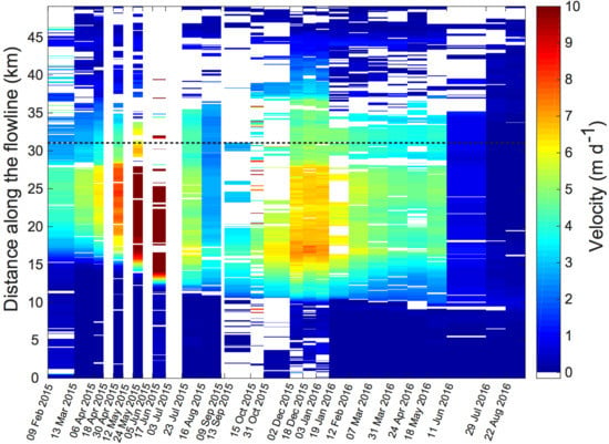
1. Introduction
The Karakoram region is well known for its surge-type glaciers [1]. In particular in the central Karakoram recently or currently actively surging glaciers are abundant (e.g., [2,3,4,5,6]). During the active phase of a typical glacier surge, large amounts of ice are rapidly (by a factor of ten or more compared to normal flow velocities) transported from a higher so-called reservoir area to a lower receiving area. After the surge, in its quiescent phase, ice flow slows or becomes stagnant allowing ice to melt away over years to decades in the new ablation area while new snow and ice accumulate in the reservoir area, building up mass for a possible next surge, (e.g., [7]). In cases where a surging glacier interacts with another glacier (i.e., as either an ephemeral or permanent tributary), surface morphological features, such as distorted or tear-dropped moraines, sometimes develop. These have been used widely to infer past surge-activity and identify surge-type glaciers in satellite imagery, (e.g., [8,9,10]).
The surges in the Karakoram show a wide range and mixture of characteristics regarding frontal advances (or not) and advance rates, surge duration, velocity increase, and mass change pattern (among others) that have recently been studied in detail using optical and SAR (Synthetic Aperture Radar) remote sensing data, (e.g., [3,5,11,12,13,14]). Glacier surges in the Karakoram also vary in regard to their interactions. For example, they can be related to isolated speed-up events within a single glacier that are difficult to distinguish from seasonal velocity variations, glaciers surging into each other as described above, mass waves travelling down-glacier faster than the surface flow velocity, the typical strong advances of the terminus over a short (months to years) or extended (decades) period of time, or a ‘response surge’ following flow-blocking release when the surge of a tributary glacier (blocking the flow of another glacier) comes to an end, (e.g., [4,6]).
Some features used for identification of surge-type glaciers, such as looped or distorted moraines, can only be observed on larger glaciers with debris cover and thus might not always exist. This can make identification of surge-type glaciers in their quiescent phase difficult and biased, as the number of identified surge-type glaciers might increase with time and increasing information availability, not least through satellite data. Analysis of satellite image time-series (or aerial photography if available) and historic reports can be helpful to reveal possible former surges [1,4,8,15], but often it is required to use several criteria for a clear identification, (e.g., [5,16]). For example, some glaciers might only show a strong increase of flow velocity without corresponding terminus advance, (e.g., [17]), or others advance at rates similar to non-surge-type glaciers (less than 100 m y−1) but do so for more than 10 or 20 years (e.g., First Feriole in the Panmah region). As it is not yet clearly defined how a surge-type glacier can be identified (cf. the list of criteria summarized by [16]), their number for a specific region will also vary with the interpretation by the analyst.
Hispar Glacier (HG) is one of the largest glaciers in the Karakoram that has reportedly so far not surged itself, (e.g., [1]), but is accounted for being impacted by surges of its tributaries. In this study we describe its 2015/16 surge using a time series of Landsat images (sensors MSS, TM, ETM+, and OLI) to derive morphological changes and pre-surge variability of flow velocity. In addition, SAR images from Sentinel-1 and RADARSAT-2 are exploited together with the optical data to derive a dense time series (about bi-weekly to monthly means) of flow velocities during the surge. Based on these results we hypothesize about a possible surge mechanism. By analyzing historic reconnaissance imagery from Corona, we also provide evidence that the middle part of HG experienced a surge around 1960.
2. Study Region
Hispar Glacier is located in the central Karakoram and drains into the Hunza catchment in Pakistan (Figure 1, inset). Its main trunk is a nearly 50 km long (area about 500 km2) linear stream of ice, flowing towards WNW from Hispar pass at 5150 m a.s.l. down to 3100 m. It is the dominant glacier in the near-linear main valley but other large surge-type glaciers (Trivor, Bualtar) drain further to the west into the main valley. A high mountain range (up to 7000 m) is protecting the ESE-WNW orientated valley in the south and the Hispar Muztagh (up to 7800 m) in the north. At Hispar pass, HG is connected to the third longest glacier in the world, the 65 km long Biafo Glacier, flowing to the East. Hispar glacier has a comparably tiny accumulation area that is not much wider than the tongue in the ablation region and is composed of three small basins. However, from the south about a dozen small tributaries nourish the tongue and from the north, three large tributary glaciers feed the main glacier trunk (Kunyang, Yutmaru and Khani Basa). The tributaries collectively contribute about a half of the total width of the main tongue and the looped/distorted medial moraines on the main glacier indicate former surge or fast-flow events.
The three northern main tributaries of HG are complex glacier systems with multiple tributaries nourishing their respective main tributaries, i.e., their shape has a sort of fractal self-similarity. Due to the high relief of their surrounding ice-free rock walls, the ablation areas of the three tributaries are also debris-covered (with decreasing amounts from Kunyang in the west to Khani Bassa in the east). The lower part of the main tongue of HG is completely debris covered and characterized by numerous supra-glacial melt ponds as well as circular collapse structures, indicating the widespread down-wasting of the tongue. The latter has been confirmed in the study by [14] for the period 2000–2008 from differencing of digital elevation models (DEMs).
Limited information is available about the climatic regime of the glacier studied as meteorological stations are sparse, their time series are often short (a few decades), and they are located at comparably low elevations [18]. Mean annual air temperature at the station Gilgit (1460 m a.s.l.) about 80 km to the west-southwest of HG are 15.8 °C [19], gives a value of about −3 °C (lapse rate −0.007 °C m−1) at the midpoint elevation (4125 m) of HG. According to [20] the region receives about the same share of precipitation in summer and autumn as in winter and spring, i.e., it is influenced by both the monsoon and westerly’s. Annual amounts are very low (e.g., in Gilgit 137 mm according to [19]) but increase with elevation to about 1 m at 4500 m a.s.l [21]. A study by [22] indicated amounts in the order of 1.2 m a−1 in the accumulation region of the neighbouring Biafo Glacier and [23] reported between 1 and 2 m at Hispar pass (5060 m a.s.l.).
Taken together, this suggests a cold continental climate and that HG could, at least in parts, be poly-thermal. A slight increase in winter precipitation and decrease in summer temperature has been reported by [18] and confirmed by [19] using nearby meteorological stations. This indicates increasingly favourable conditions (in mass balance terms) for glacier survival. The related balanced to slightly positive mass budgets over the 2000 to 2010 decade have been confirmed by several studies that analysed glacier elevation changes, independent of surge-type glaciers being in the sample or not, (e.g., [14,24]). A comparison with historic maps and early photographs of the terminus reveal limited changes in terminus position of HG over the past 120 years. This also indicates nearly balanced mass budgets over this time period, and several decades before.
3. Data Sets and Image Processing Methods
3.1. Data Sets
Two types of satellite images have been used in this study: (1) Optical images from the Landsat series and Corona to (a) illustrate and interpret historic as well as recent changes of HG in a more qualitative and geomorphologic sense, and (b) to derive flow velocities (only Landsat); and (2) time-series from SAR sensors (Sentinel-1/RADARSAT-2) that have been acquired during the surge were used to derive surface flow velocities with high temporal resolution. The satellite images used are listed in Appendix B Table A1 (animation), Table A2 (pre-surge) and Table A3 (main-surge). High-resolution (about 5 m) Corona scenes from 1965 and 1969 were used to identify the surface morphology of HG prior to 1977, when a Landsat MSS scene with very good quality is available. After 1990 Landsat scenes are available every 2–3 years.
For the 2015/16 surge period a Landsat 7/8 time series could be obtained to follow the evolution of the surge visually (see Table A1). We have created an image series from these scenes (Supplemental File S1) that can be animated to reveal the dynamics of the surge [4]. As some images have fresh snow-cover, stripes from Landsat 7 SLC-off scenes, and clouds, all creating strong changes in contrast, it is recommended to focus viewing on the surging parts of the glacier tongue. All images are derived from the standardized image quicklooks provided by USGS (e.g., glovis.usgs.gov). They have a somewhat reduced quality (jpg-compression) compared to the original data but the advantage of homogenous contrast and colours, which facilitates visual interpretation of the animations.
To derive flow velocities, the original panchromatic bands from Landsat 7 ETM+ and Landsat 8 OLI (15 m resolution) have been used. Landsat data were freely downloaded from the website earthexplorer.usgs.gov. The Sentinel 1 images were provided by ESA and obtained from the Sentinel Science Hub (scihub.copernicus.eu). The RADARSAT-2 scenes were provided by the Canadian Space Agency (see Acknowledgments).
For comparison with current glacier extents and surface morphology, we have also analysed the historic map from the Bullock-Workmann expedition in 1908 that is available online. We used glacier outlines for the region as available from the Randolph Glacier Inventory (RGI) version 5.0 [25] to spatially constrain the analysis of the flow velocities, assign regions of stable ground for uncertainty assessment of flow velocities, and for visualisation of glacier extent.
3.2. Methods
Feature tracking of 19 Landsat 7 ETM+ scenes and 14 Landsat 8 OLI scenes (panchromatic band with 15 m spatial resolution) acquired between July 2013 and January 2016 was performed using the CIAS software [26,27]. We used the orientation correlation function to extract displacements with a reference block size of 15 pixels (225 m), a search area size of 50 pixels (750 m) at a grid of 100 m. Table 1 provides the parameters used for the tracking algorithm.
Three RADARSAT-2 Wide Fine (RS-2 WF) scenes were acquired between December 2014 and February 2015. These repeat data were used to retrieve two glacier surface velocity maps using the offset tracking method of the GAMMA software [28]. The size of the correlation matching window was adjusted according to the image resolution and expected maximum displacements during the repeat pass cycle to 38 × 77 pixels in range and azimuth (see Table 1). The resulting RS-2 velocity maps were then geocoded using the SRTM DEM to a 100 m resolution raster.
A series of Sentinel-1 Interferometric Wide Swath (IWS) images were acquired between March 2015 and December 2016 along both ascending and descending orbits (Appendix B Table A3). The repeat Sentinel-1 IWS data were used to retrieve a time-series of surface velocity maps using the offset tracking method of the GAMMA software [28] (see Table 1 for parameters). Slant-range and azimuth offset-fields were combined to retrieve horizontal surface velocity maps. These were geocoded using the SRTM DEM at a 100 m resolution raster.
The Corona images were only analysed qualitatively and not geocoded. All Landsat satellite images were used as is, i.e., terrain corrected by USGS (Level 1T). Mismatches and outliers were identified and removed from the velocity maps using different tests. For the Sentinel 1 and RADARSAT-2 data the signal-to-noise ratio had to be above 2.0 to result in a valid match. Landsat velocity maps were filtered with a standard deviation filter. Values are defined as outlier when the standard deviation of a pixel in a 3 × 3 window surrounding it exceeded 32 m. Moreover, in all maps values above 15 m d−1 (the maximum flow velocity) were removed. The accuracy of the derived velocity fields for Sentinel-1 was estimated from the displacement over stable terrain (using the RGI glacier outlines as a mask and restricting calculations to flat terrain.
To follow the spatio-temporal development of flow velocities in more detail, we manually digitized three centre lines: one along the main glacier and two for its middle and eastern tributaries. These were converted to points with discrete IDs and a distance of 50 m (see Figure 1). Their coordinates and IDs were exported to a csv file and used in a small script for automated extraction of values from the computed velocity fields. Resulting values were organized and further processed for visualisation. Values for the eastern tributary (Khani Bassa) are not shown as the analysis revealed that it did not participate in the surge studied here.
4. Results
4.1. Historic Development of Hispar Glacier from Landsat Data
The surface changes of HG from the available historic satellite data from Landsat (sensors MSS/TM/ETM+/OLI) reveal some interesting details about its past development, all of which are not obvious from its stagnant terminus, geodetic volume changes or analysis of flow velocities. Figure 2 shows a time series of the glacier surface from 1977 (MSS), 1990 (TM), 2013 (OLI) and 2015 (ETM+) with some characteristic features marked by arrows with different colours. Through the full near 40-year time series the terminus position has not changed (green arrow at top left). Characteristic surface features (distorted moraines) indicated by yellow, white and orange arrows move slowly down-glacier from 1977 to 2013, with a somewhat higher velocity in the upper glacier regions (larger displacement of the yellow arrow). In total, five of such marks are visible in the 1977 MSS image (Figure 2a) indicating previous disturbances of the flow. A prominent moraine distortion (without arrow in the figure) at the confluence with Pumarikish Glacier (Figure 2a) was destroyed by its 1989 surge [29] that is marked by a white circle on Figure 2b. Another surge mark to the east of the confluences with Kunyang Glacier is still visible in the 1990 image but no longer present in 2013 (Figure 2c).
Further extracts from the time-series of Landsat images reveal that Kunyang Glacier started to surge in 2006 and advanced into HG in 2008 with some further advance until 2009. This surge is also visible in Figure 9 of the study by [14] in which they calculated DEM differences between 1999 (from SRTM) and 2008 (from SPOT). In the 2013 image (Figure 2c) the glacier is again in its quiescent phase, but the marks of the surge are still recognizable by its lobate form, covering about 3/4 of the width of HG. The good contrast in the 2013 image reveals the exposed northern lateral moraine (shorter black arrows), indicating that the glacier surface had been previously higher.
4.2. The 2015/16 Surge from Optical Images
When contrasting the appearance of the autumn 2015 glacier surface (Figure 2d) with the appearance in 2013 (Figure 2c), strong changes can be recognized. Most prominent is the reduced debris load due to the increased crevassing (indicated by the more “bluish” surface in regions marked by the light blue arrows) for both HG and its tributary Yutmaru Glacier. The synchronous surge of both glaciers is supported by the stable position of the medial moraine between them (if Yutmaru had surged onto HG, the moraine should have been translated and deformed). One can also recognize the lateral expansion of the tongue and the increased ice thickness (the lateral moraine in the 2013 image disappeared), along with the forward movement of the surface marks (large orange and white arrows). Further downstream the surge front can be identified (light blue line with half elliptical shape in Figure 2d). The lakes west of the orange arrow in the 2013 image have disappeared. The animation of the 2015/16 Landsat images (see Table A1) clearly reveals a mass wave with a related surge front travelling down glacier in 2015/16. The surge front stopped before the confluence with Kunyang Glacier that is still occupying about 3/4 of the width of HG.
4.3. Flow Velocities before, during and after the Surge
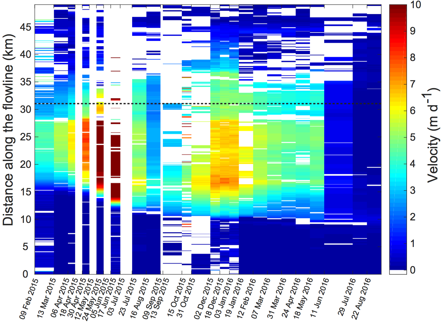
In Figure 3, Figure 4, Figure 5 and Figure 6 we show the temporal evolution of flow velocities before the surge as derived from time-series of Landsat images (Figure 3 and Figure 4) and during/after the surge from time series of Landsat and Sentinel-1 images (Figure 5 and Figure 6). Results from RADARSAT-2 are not shown as the Landsat time series had a better quality. The figures show either the full flow field from selected image pairs of the time series (Figure 3 and Figure 5) or mean values along a central flow line of HG in time-distance plots with velocities colour coded (Figure 4 and Figure 6). In the latter two, the red-brown horizontal line notes the position where the Yutmaru tributary joins the flow of HG.
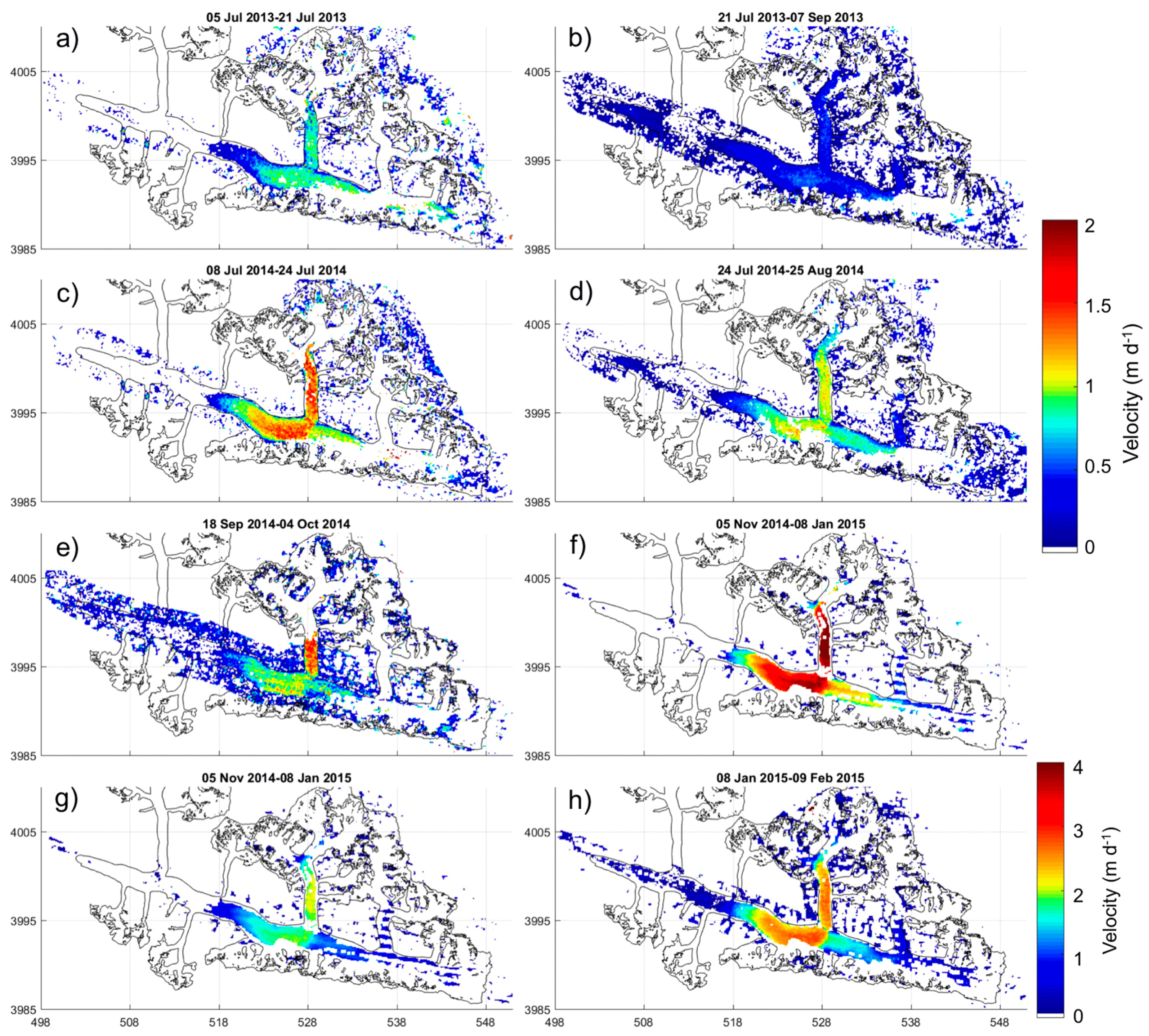
The first two image pairs in Figure 3 show the summer speed-up and slow-down in July and August of 2013 (Figure 3a,b) and 2014 (Figure 3c,d). Although difficult to see due to data voids, these velocity increases reach beyond the eastern tributary well into the accumulation area of HG. Notably, the summer speed-up in 2014 reached peak velocities twice as high as in 2013 (nearly 2 m d−1 instead of 1 m d−1). Interestingly, Figure 3e shows an increase in flow velocities for the Yutmaru tributary in September 2014 instead of a further slowdown as in 2013. This increase has seemingly activated the ice of HG, which is still in its summer-mode of increased speed, as Figure 3f shows flow velocities exceeding 2 m d−1 for both HG and Yutmaru Glacier in November/December 2014.
This result is shown again in Figure 3g but with an extended colour scale (max. is now 4 m d−1) to reveal the further flow acceleration during January 2015 to 4 m d−1 (Figure 3h). The related time-distance plot in Figure 4 confirms the up and down of velocities with additional time slices. From October 2013 to January 2014 flow velocities are indeed below 0.4 m d−1 (or 150 m a−1). The massive increase in flow velocities after the surge started in October 2014 is well visible for the last two image pairs from December 2014 and January 2015. From these plots it seems that the surge started beyond the confluence region with Yutmaru (at km 31) and increased flow velocities occurred also backwards towards the accumulation region.
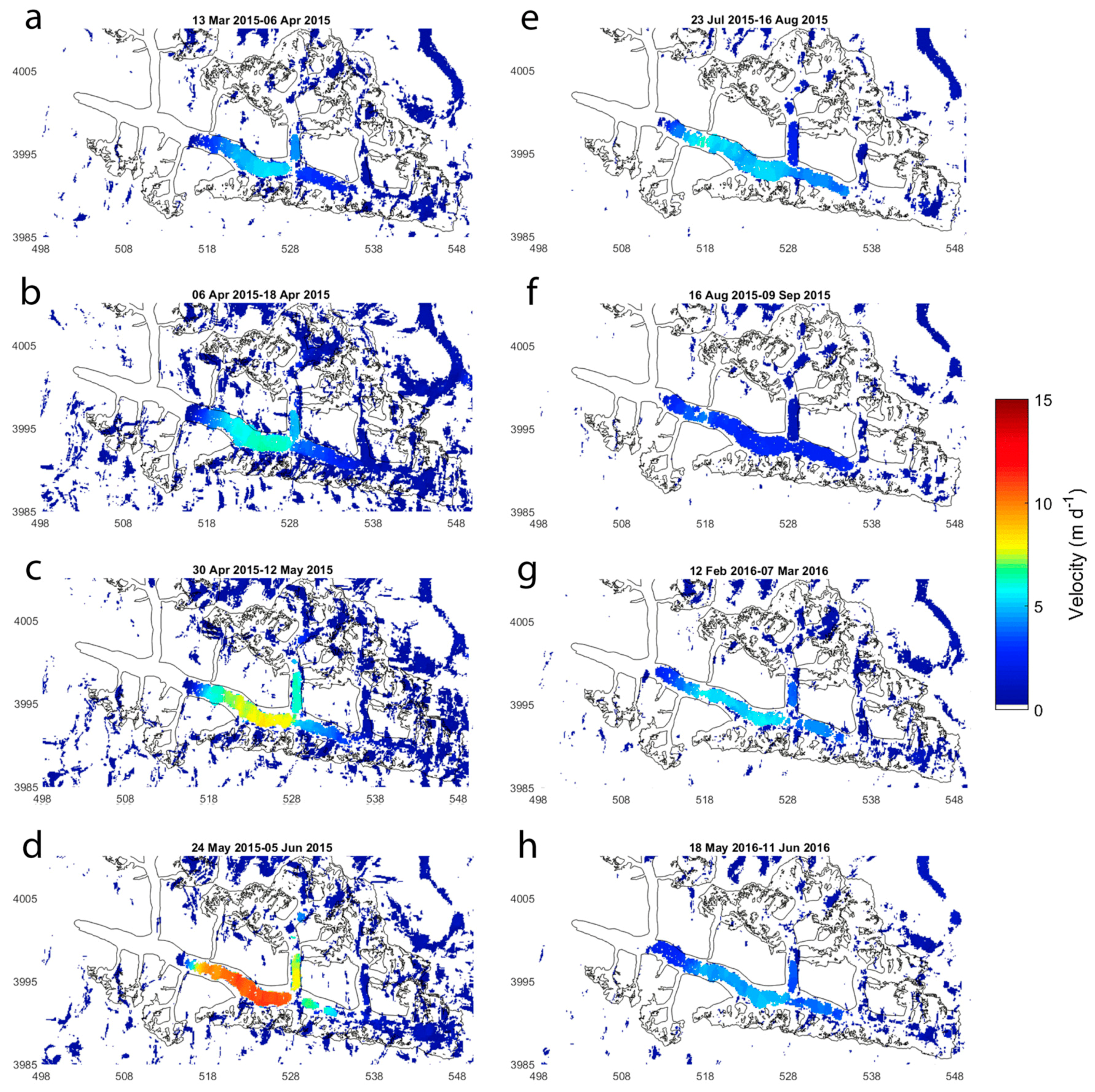
In Figure 5 the evolution of surface flow velocities from March 2015 to June 2016 is shown based on time series of Sentinel-1 images. Velocities increased to about 6 m d−1 in April 2015 (Figure 5b) and 7 m d−1 until mid-May (Figure 5c). Flow velocities of the Yutmaru tributary are already much lower then and it looks like the surge is just originating in the centre of HG. Flow velocities downstream of the confluence area nearly doubled to about 14 m d−1 (about 5 km y−1) until the end of May (Figure 5d) and dropped to 5 m d−1 (Figure 5e) and less than 2 m d−1 (Figure 5f) by the end of July and August, respectively. During winter and spring 2016 flow velocities for the main glacier increased again to about 7 m d−1 (Figure 5g,h) before they sharply dropped to less than 1 m d−1 by July 2016. This dual surge with the sharp drop can also be seen in the time-distance plot of Figure 6. In this figure, we have restricted maximum velocities to 10 m d−1 to reveal details in the second surge pulse. Apart from the sudden drop in flow velocities the most interesting aspect is a very subtle one—the advance of the surge front. For the three image pairs acquired at the beginning of May, end of May and end of June of 2015 the zone with speeds of around 6 m d−1 (yellow area in Figure 6) moved in about 25 days by about 2–2.5 km or about 90 m d−1. The rapid advance of the surge front could thus be related to a kinematic wave or some other mechanism near the glacier bed that has activated the flow.
The scatterplot showing flow velocities against distance from the terminus and colour-coded for time (Figure 7) confirms this evolution but shows the rapid advance of the surge front more clearly. The point separating the regions of fast and slow flow rests more or less at the same place (at km 15) until April 2015. Flow velocities increased to about 2.5 km a−1 (about 7 m d−1) behind this point before it advanced by nearly 5 km in 2 months. The scatter plot also shows the drop in flow velocities where the two tributaries Yutmaru (km 28) and Khani Basa (km 35) join the flow. The part between the two confluence points (upstream of Yutmaru) takes part in the surge (though on a lower level) whereas the part upstream of Khani Basa confluence did not. During the period with the highest flow velocities there is a ±500 m a−1 (1.4 m d−1) variability of flow velocities between km 15 and 28, even in this smoothed display (averaged over 200 m bins). However, in view of potential measurement uncertainties this variability is likely within the error bounds and should thus not be over interpreted. In contrast to the dynamics of the upper glacier parts that are influenced by the surge, flow velocities for the nearly stagnant lower part of the tongue are below 30 m a−1.
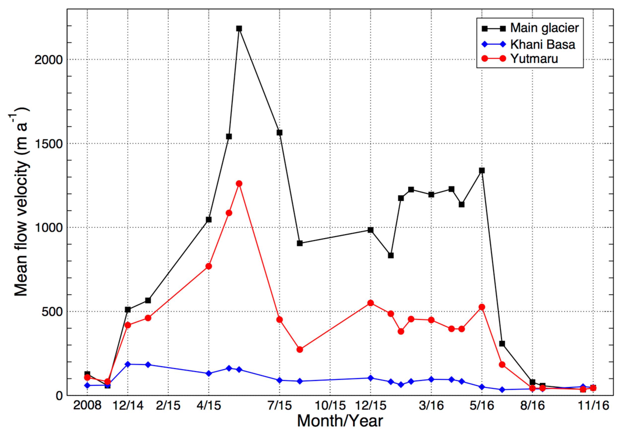
Flow velocities along the profile of the Yutmaru tributary change in the same way as the main glacier but are in general somewhat lower as can be seen in Figure 3. To get a better overview on the temporal development of flow velocities for the main glacier and the two tributaries, we have also calculated velocity averages along the flow lines, excluding the data gaps and starting at km 14 for the flow line on HG. When plotting these averaged velocities for the three major flow lines against time (Figure 8), the main variability emerges. Flow velocities show a continuous acceleration from Autumn 2014 to May 2015 for both HG and the Yutmaru tributary followed by a massive drop in Summer 2015. Velocities stayed at this level until January 2016 for HG but slightly increased for Yutmaru. Mean velocities increased for HG in February 2016 and stayed at this level before they suddenly dropped in June 2016. Yutmaru has about constant flow velocities from December 2015 to May 2016. Although the mean values given in Figure 6 are somewhat arbitrary, one can roughly say that averaged flow velocities of the Yutmaru tributary at and after the peak in May 2015 are about half of the HG values. The eastern tributary (Khani Basa) shows a small increase in flow velocity in Dec 2014, but constantly declined afterwards. At a closer view, there is a little bit of up and down that is synchronous with the variability of the two other glaciers.
4.4. Accuracy of the Derived Flow Velocities
The displacement over stable terrain for Sentinel-1 gives on average values of about 13 m a−1 with a standard deviation of 20 m a−1 (18.3 for descending, 21.9 for ascending orbits) in the mean over all processed scenes. This is about two orders of magnitude smaller than the observed displacements and should thus have no impact on the results. Similarly, a recent study by [30] found in comparison to higher resolution sensors a displacement error of about 30 m a−1 for Sentinel-1 interferometric wide swath (IWS) images with 12 days repeat, and 15 m a−1 for RADARSAT-2 Wide Ultra Fine (WUF) images over a 24 days period. Uncertainties for Landsat-derived velocities are similar to previous investigations (e.g., [31,32,33]), revealing displacement accuracies of one pixel or better, i.e., 15 m for Landsat 8, or 1 m d−1 for 16-day repeat [27,34].
5. Discussion
5.1. Interpretation of the Observations
Based on the available optical and SAR datasets, the observed geomorphometric changes, and the spatio-temporal variability of the flow velocities, it seems that the 2015/16 surge of HG started at the confluence region of HG and Yutmaru glacier in October 2014, with steadily increasing flow velocities (up to 5 km a−1 or 14 m d−1) until May 2015. At about the same time, the previously stagnant surge front started to move forward by about 5 km in about two months. Flow velocities quickly dropped by about one half in summer 2015 and stayed at this level until winter 2015 before they slightly increased again in spring 2016. The final drop in speeds back to pre-surge values was strong and fast (see Figure 8).
Taken together, this seems to be a surge of Alaska-type that is controlled by the hydrologic regime, (e.g., [7,35]). The build-up during winter 2014/15 points to an acceleration due to increased basal water pressure resulting from an ineffective basal drainage system (linked cavities). This pressure could have been strongly reduced after basal flow became more efficient during the summer (connected channels), causing the first strong decrease in flow velocity. However, velocities remained high during summer/autumn 2015 when basal sliding was maybe increased due to water generated by friction from the high flow velocities, additional meltwater input, or the water drainage system constantly being destroyed by the high basal deformation. The second winter/spring increase of flow velocities indicates that basal drainage was getting even more inefficient again and water pressure increased, before drainage changed again to the more efficient channelized mode in summer 2016, terminating the surge. A speed-up in the flow during winter and spring has also been observed at other surging glaciers, (e.g., [5,7,15,36]) and hints to a common hydrologic cause for the observed timing of the surge. The observed seasonal variability before the surge is much lower in magnitude, influenced larger parts of the main glacier and had a different timing (highest velocities in summer). Regarding the double peak of flow velocities and the sudden drop at the end of the surge (see Figure 8) we find some resemblance with the 2015 surge of Kyagar Glacier which is located to the north east in the Shaksgam valley and described by [37]. However, for Kyagar Glacier maximum velocities were much lower (2 m d−1) and reached in September. So, its surge mechanism might be different. A speed up in flow during winter was also observed by [38] for the West Kunlun Glacier, but we assume that the surge mechanism is different here as the glacier is at least poly-thermal if not cold based.
The surge of HG started in October 2014 during the autumn deceleration phase and was probably initiated by a flow acceleration (or maybe a surge?) of Yutmaru Glacier (Figure 3e). In contrast to other glaciers where surging tributaries deform medial moraines of a main glacier (e.g., Panmah or Skamri glaciers), the acceleration of Yutmaru did not deform the medial moraine of HG. Instead, HG immediately started to surge itself with about the same flow velocity (Figure 3f,h). We speculate that the reason for this quick response is related to its still higher than normal summer flow velocity with considerable lubrication at the bed. The region with the increased flow velocities is identical with the region of faster flow before the surge (cf. Figure 3e,f). But already in January 2015 the region upstream of the confluence region had much lower flow velocities. This early ‘decoupling’ can also be seen in Figure 8. For the Yutmaru tributary the decoupling took place by the end of April 2015 (Figure 5c) before the maximum flow velocities were reached. Considering that Yutmaru Glacier only provided a small push to HG before its surge started suggests that HG was ready to surge before, but a trigger was missing. It is also noteworthy that for a considerable time of flow acceleration (1/2 year) there was no forward movement of the surge front. This happened only after maximum flow velocities were reached in May/June 2015. By then, a considerable amount of ice accumulated upstream before it could finally break through and the mass wave visible in the satellite animation started to travel downward at high velocities. There is maybe an obstacle at the bed at km 15 that is difficult to pass.
5.2. Is the Surge Unprecedented?
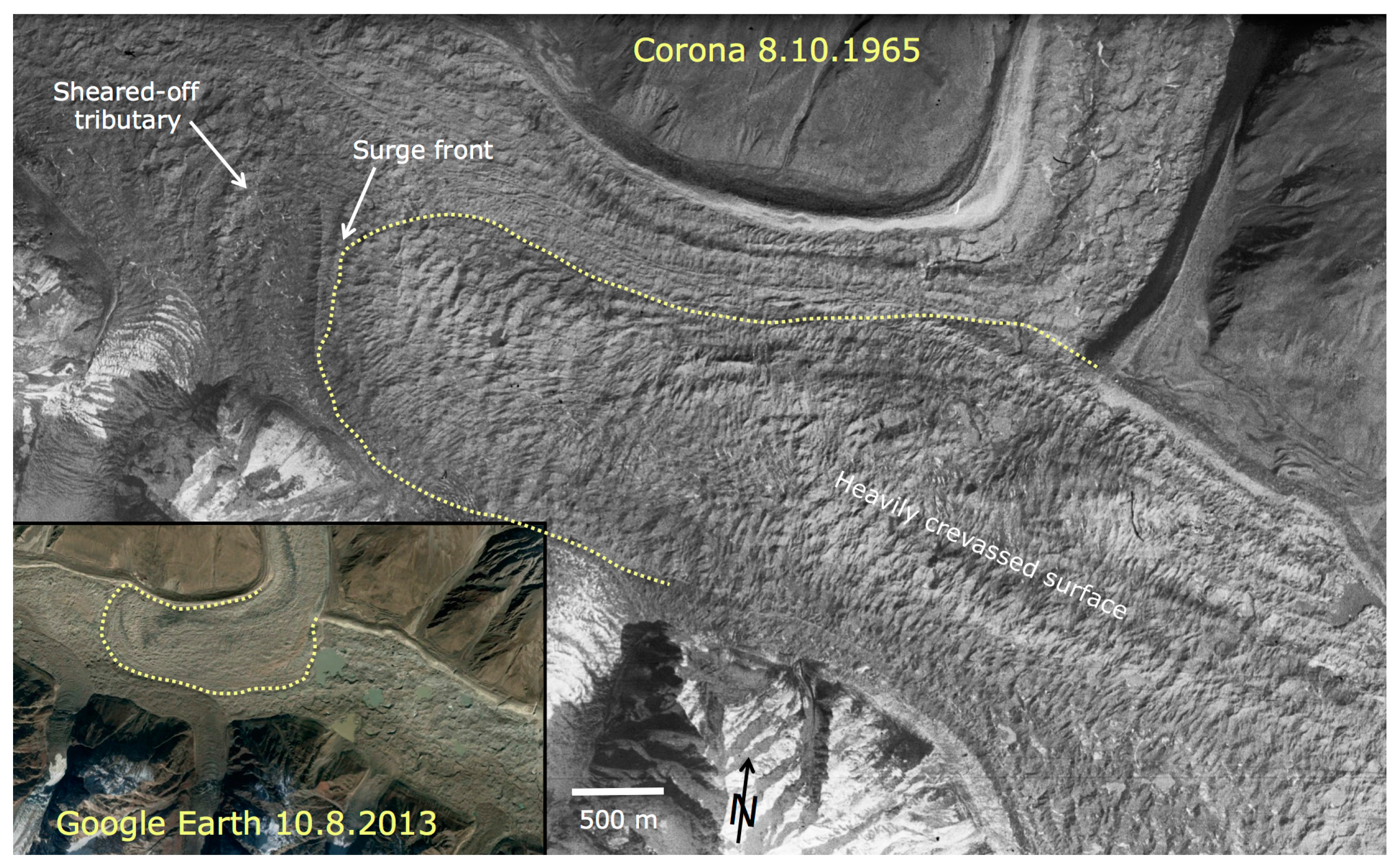
Going further back in time, there are no reports of a surging HG from the 19th and 20th century [1] and early topographic maps of the glacier surveyed in 1892 by W. Martin Conway and in 1908 by the Bullock-Workmann expedition do also not show any signs of irregular flow. Medial moraines are lined up in parallel and overall the glacier seems to have less debris cover than nowadays. However, there is one source indicating a possible previous surge of the main HG, a Corona image from 1965 (Figure 9). This image with a spatial resolution of a few metres shows a chaotic and highly crevassed surface typical of a glacier surface a few years after a surge. On that image one can also see that the Kunyang Glacier tributary—that is now occupying 3/4 of the valley width—was nearly completely pushed away and occupied less than 20% of the width of the main valley. A well visible surge front is indicating that this ‘surge’ reached about 4 km further downstream compared to the 2015/16 surge but has also not reached the terminus.
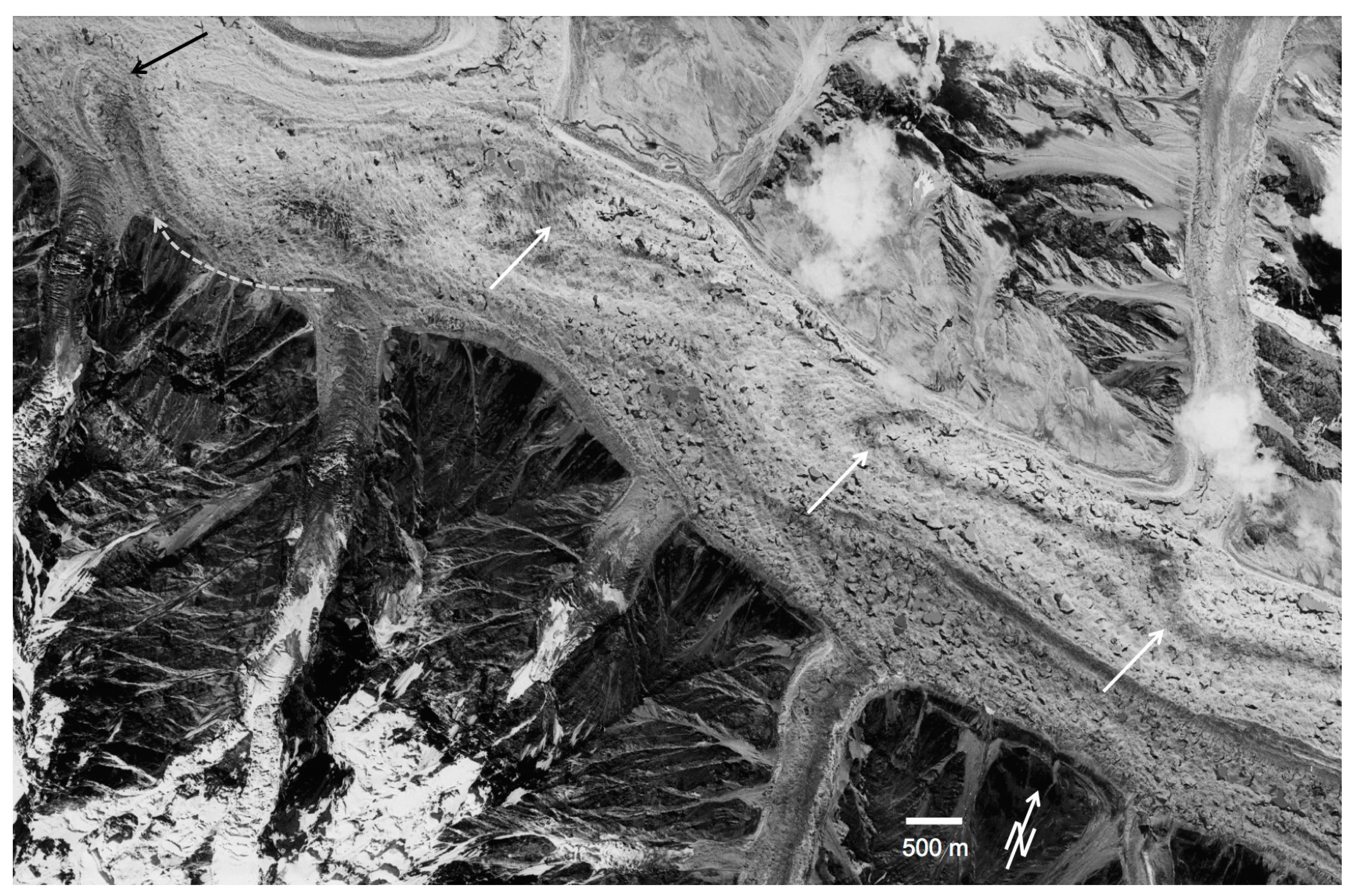
About four years later, another Corona image reveals an impressive change of the surface morphology (Appendix A, Figure A1). Whereas the extent of the former surge is still well visible, the surface is strongly smoothed and the previous crevasses are barely visible. Instead, the entire surface is covered with (partly water-filled) depressions and sinkholes, indicating a massive down-wasting and collapse, which is a typical post-surge phenomenon when the surged ice mass becomes stagnant. The limited movement after the surge is also supported by three surge marks (loops and distorted moraines) that are in 1977 (MSS image in Figure 2a) in the same position as in 1969 (they are located in front of Pumarikish and Kunyang glaciers). Interestingly, Kunyang Glacier in 1977 is again occupying about 50% of the valley width, indicating that the down-wasting post-surge ice mass of Hispar Glacier could be easily pushed away. The Corona image from 1969 (Figure A1) also shows a lobate, dual-coloured surge mark before the surge front, indicating that this former surge (it might have taken place around 1960, i.e., 55 years before the current surge) might have sheared of the lower part of a southern tributary, likely from Gandar Glacier (see Figure 2a), which both have a dual-shaded moraine. In the latter case, the surge would have also started at km 15 and must have travelled at least 9 km downstream. Finally, a recent study by [39] showed elevation differences from 1973 to 1999 using DEMs derived from Hexagon KH-9 stereo pairs and SRTM for the Hunza catchment. In this study HG shows a strongly down-wasting middle section that is compliant with the extent of the surge and the typical post-surge down-wasting described before from the morphological change. So the 2015/16 surge of HG seems not unprecedented but has at least one precursor.
The teardrop-shaped moraine distortions visible in Figure 2a and Figure A1 indicate that additional surges of HG should have happened in the past as each loop has to be created and pushed forward by a separate surge (or fast flow event). The only obvious glacier upstream of Kunyang being able to create the flow distortions of the main glacier is Yutmaru. The three surge marks suggest that Yutmaru had at least three periods with unstable flow that slightly deformed the medial moraine and—different from the here-reported event—might have partly blocked the flow of HG. Considering their elongated/stretched shape and the very low flow velocities of HG during its quiescent phase (see Figure 2), it can be assumed that HG has responded to this partial flow-blocking also with a surge (or fast-flow event) that pushed the surge marks forward into their current elongated (tear-drop) shape. Apart from the 1960s event suggested by the Corona images we do not know when these former surges might have happened. For comparison, the Sentinel-2A image in Figure A2 shows how HG looks shortly after the current surge ended.
5.3. Interpretation of Observations
Our interpretation of the observed temporal evolution of flow velocities and geomorphological evidence is largely based on a translation of what has been reported and observed in previous studies to the case of HG. We think that the assumption that changes in basal hydrology had a major impact on the variability in flow velocities is robust and not unexpected, as this has been reported for other surging glaciers with a sub-seasonal analysis of flow velocities [15,32]. Our assumption that HG was ready to surge and just “waited” for a trigger to start it is more speculative, but we think reasonable in view of the observations. However, our interpretation does not necessarily mean that the surge mechanism for HG works exactly as we speculate. Further research and additional observations (e.g., elevation changes) would be required to improve on the current (limited) understanding, in particular when considering that other surging glaciers in the region show a very different behaviour (e.g., the continuous advance over 15 years of First Feriole Glacier).
Our speculation about former surges of HG and its Yutmaru tributary are based on analysing time series of historic satellite images (Corona, Landsat). They are supported by multiple lines of evidence and are fully compliant with what has been observed elsewhere in terms of surge marks, looped moraines, crevasse decay patterns and surface elevation changes. We thus think our interpretation is robust in this regard. Together with Skamri Glacier to the north-east, HG is thus one of the largest surging glacier in the Karakoram. It is likely that further surge-type glaciers will be identified in the future based on their sudden change in surface flow, and new interpretation of surge marks and historic evidence. Thereby, the high temporal resolution of the current satellite coverage (Sentinel-1/2 every 5–6 days, Landsat 7/8 every 8 days) will likely also help reveal potential surge mechanisms and thus improve our understanding of this fascinating phenomenon.
6. Conclusions
We presented a detailed description of the 2015/16 surge of Hispar Glacier as derived from the qualitative interpretation of optical image time series (Corona, Landsat) and the quantitative determination of flow velocities from both optical (Landsat 7 and 8) and SAR images (Sentinel-1 time series). Whereas the optical images allowed us to obtain pre-surge variability and the onset of the surge, the dense time series (partly every 2 weeks) of Sentinel-1 images allowed us to follow the spatio-temporal development of the surge in detail. The surge started in autumn 2014 and peaked with surface flow velocities of up-to 5 km a−1 (14 m d−1) over a short period in May/June 2015. During summer 2015 maximum velocities decreased substantially before they increased again in winter 2015/16. In June 2016 the surge ended abruptly. We assume that the variability of velocities over the full almost two-year duration of the surge are related to changes in the basal hydrologic regime and would thus classify the surge as Alaskan type.
The most interesting aspects of the surge are: (1) the near-synchronous surge of HG and its tributary Yutmaru, (2) the stationary surge front (for 6 months), and (3) the high velocities of the surge front (up to 90 m d−1) once it started moving down-glacier. We interpret an end-of-summer fast-flow event of the Yutmaru tributary as a trigger of the main HG surge that was likely “ready to go” before. We do not know what kept the surge front stationary for half a year but interpret its rapid advance afterwards as a kinematic wave travelling down-glacier about six times faster than the maximum flow velocity.
So far, surges have only been reported for some of the HG tributaries (Kunyang, Pumarikish) but not for HG itself. We have shown here that HG has very likely also surged around 1960 and maybe also before. None of these surges seem to have reached the terminus that has been stationary for >120 years according to the literature and historic maps. The high temporal resolution of satellite images now available will likely reveal similar details of surge evolution for other glaciers and contribute to an improved understanding of glacier surges.
Supplementary Materials
The following are available online at www.mdpi.com/2072-4292/9/9/888/s1, Animation S1: Hispar Glacier surge (zip file with individual images).
Acknowledgments
This study has been performed in the framework of the ESA project Glaciers_cci (4000109873/14/I-NB). T.S. was funded by the Norwegian Space Centre as part of European Space Agency’s PRODEX program (C4000106033), and the European Union FP7 ERC project ICEMASS (320816). A.K. also received funding from the European Union FP7 ERC project ICEMASS (320816) and the ESA project Glaciers_cci (4000109873/14/I-NB). RADARSAT-2 data was provided by the Canadian Space Agency under the proposal SOAR-EI 5166. Glacier outlines were obtained from the Randolph Glacier Inventory (RGI5.0).
Author Contributions
F.P. conceived and designed the study, wrote the paper, and analysed the results. T.S. processed all Sentinel-1 data, T.S. processed most of the Landsat and all RADARSAT-2 data and created the velocity plots in Figure 3, Figure 4, Figure 5 and Figure 6, A.K. processed further Landsat data. All authors contributed to the interpretation of the results and the writing and editing of the manuscript.
Conflicts of Interest
The authors declare no conflict of interest.
Abbreviations
The following abbreviations are used in this paper:
| a.s.l. | above sea level |
| csv | comma separated values |
| DEM | Digital Elevation Model |
| ETM+ | Enhanced Thematic Mapper Plus |
| HG | Hispar Glacier |
| RADAR | RAdio Detection And Ranging |
| RGB | Red, Green, and Blue |
| MSS | Multispectral Scanner |
| SAR | Synthetic Aperture Radar |
| SLC | Scan-line-corrector |
| SRTM | Shuttle Radar Topography Mission |
| TM | Thematic Mapper |
| USGS | United States Geological Survey |
Appendix A
Figure A1.
Corona image from 1969 showing the closure of crevasses, multiple surface lakes and collapse structures typical of a down-wasting glacier surface. Three dark-banded surge marks from previous surges can be seen in the brighter part of the surface debris cover (white arrows). The black arrow is pointing to the dual-shaded surge mark that might have been sheared-off from Gandar glacier (dashed grey arrow).

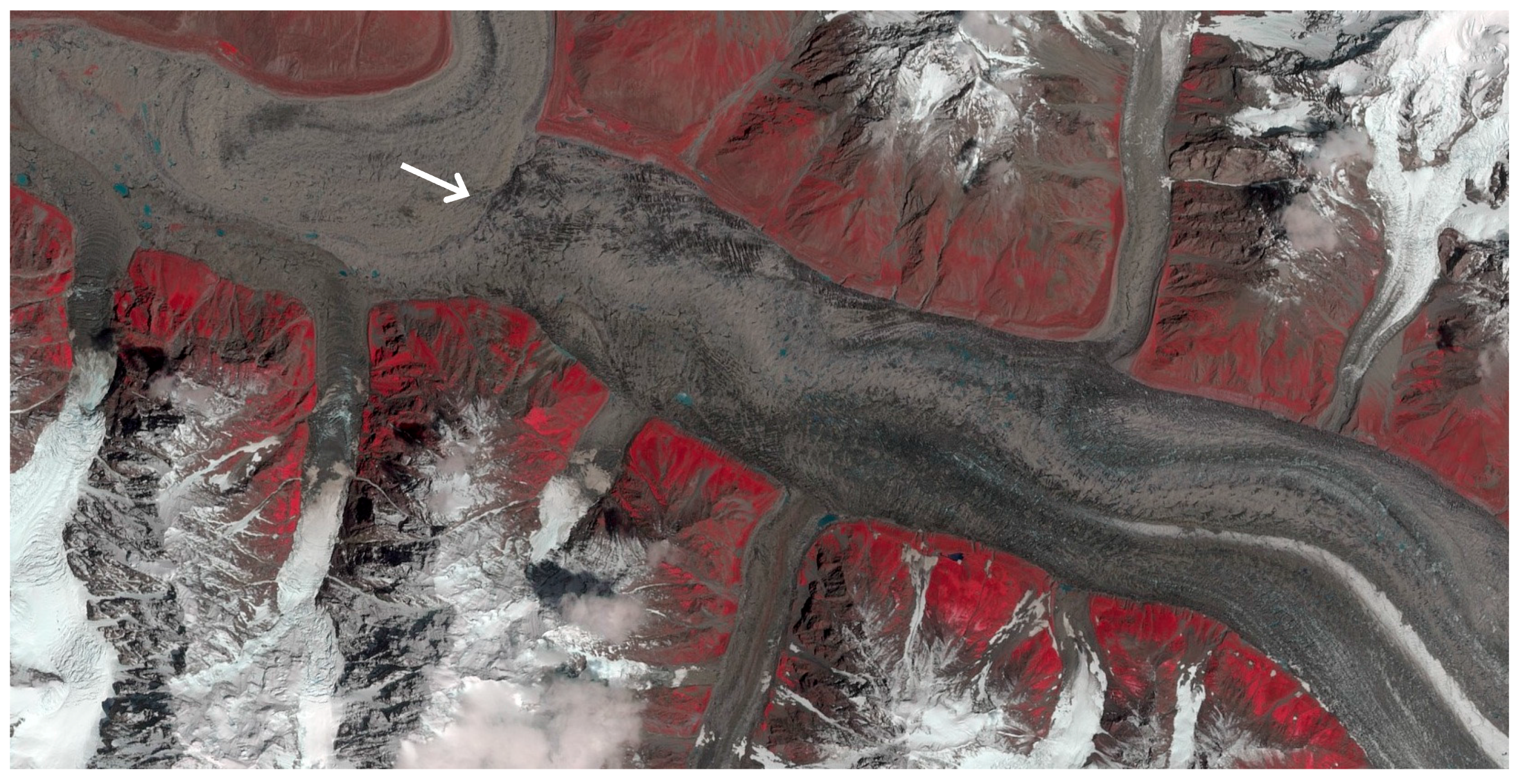
Figure A2.
The middle part of Hispar Glacier at the end of the surge. The surge front (arrow) is located before the confluence region with Kunyang Glacier. Sentinel 2A image from 20 July 2016 with bands 8, 4, and 3 as RGB (showing vegetation in red). Copernicus Sentinel data 2016.
Figure A2.
The middle part of Hispar Glacier at the end of the surge. The surge front (arrow) is located before the confluence region with Kunyang Glacier. Sentinel 2A image from 20 July 2016 with bands 8, 4, and 3 as RGB (showing vegetation in red). Copernicus Sentinel data 2016.
Appendix B

Table A1.
Scenes used for the time series in the supplement (ID 1 to 12) and Figure 2 (IDs 1, 8, 13, 14). DoY is Day of Year.
Table A1.
Scenes used for the time series in the supplement (ID 1 to 12) and Figure 2 (IDs 1, 8, 13, 14). DoY is Day of Year.
| ID | Sensor | Date | DoY | ID | Sensor | Date | DoY |
|---|---|---|---|---|---|---|---|
| 1 | L8 OLI | 9 October 2013 | 282 | 8 | L7 ETM+ | 20 August 2015 | 232 |
| 2 | L8 OLI | 25 August 2014 | 237 | 9 | L8 OLI | 13 September 2015 | 256 |
| 3 | L8 OLI | 26 September 2014 | 269 | 10 | L8 OLI | 15 October 2015 | 288 |
| 4 | L8 OLI | 16 January 2015 | 16 | 11 | L8 OLI | 10 May 2016 | 131 |
| 5 | L8 OLI | 21 March 2015 | 80 | 12 | L8 OLI | 26 May 2016 | 147 |
| 6 | L8 OLI | 22 April 2015 | 112 | 13 | MSS | 2 August 1977 | 214 |
| 7 | L8 OLI | 9 June 2015 | 160 | 14 | TM | 7 August 1990 | 219 |
Table A2.
Landsat 7/8 (ETM+/OLI) acquisitions of Hispar glacier used to derive the velocity fields depicted in Figure 3 (as indicated) and Figure 4 (all pairs). The time between two acquisitions is ∆t.
| Date 1 | Date 2 | ∆t | Sensor | Figure | Date 1 | Date 2 | ∆t | Sensor | Figure |
|---|---|---|---|---|---|---|---|---|---|
| 5 July 2013 | 21 July 2013 | 16 | L8 OLI | 3a | 29 January 2014 | 3 April 2014 | 64 | L8 OLI | |
| 21 July 2013 | 7 September 2013 | 48 | L8 OLI | 3b | 3 April 2014 | 6 June 2014 | 64 | L8 OLI | |
| 7 September 2013 | 9 October 2013 | 32 | L8 OLI | 6 June 2014 | 8 July 2014 | 32 | L8 OLI | ||
| 9 October 2013 | 25 October 2013 | 16 | L8 OLI | 8 July 2014 | 24 July 2014 | 16 | L8 OLI | 3c | |
| 25 October 2013 | 10 November 2013 | 16 | L8 OLI | 24 July 2014 | 25 August 2014 | 32 | L8 OLI | 3d | |
| 10 November 2013 | 26 November 2013 | 16 | L8 OLI | 25 August 2014 | 5 November 2014 | 16 | L8 OLI | 3e | |
| 26 November 2013 | 12 December 2013 | 16 | L8 OLI | 5 November 2014 | 8 January 2015 | 64 | L7 ETM+ | 3f/g | |
| 12 December 2013 | 29 January 2014 | 48 | L8 OLI | 8 January 2015 | 9 February 2015 | 32 | L7 ETM+ | 3h |
Table A3.
Image pairs from Landsat 7/8 (L7/L8) and Sentinel-1 (S1) descending orbits used to calculate velocities in the main surge phase (Figure 5 and Figure 6). The time between two acquisitions (in days) is ∆t. The eight scenes marked in italics are used for Figure 5.
| Date 1 | Date 2 | ∆t | Sensor | Date 1 | Date 2 | ∆t | Sensor |
|---|---|---|---|---|---|---|---|
| 13 March 15 | 6 April 15 | 24 | Sentinel-1 | 18 December 15 | 3 January 16 | 16 | L8 OLI |
| 6 April 15 | 18 April 15 | 12 | Sentinel-1 | 3 January 16 | 19 January 16 | 16 | L8 OLI |
| 30 April 15 | 12 May 15 | 12 | Sentinel-1 | 19 January 16 | 12 February 16 | 24 | Sentinel-1 |
| 24 May 15 | 5 June 15 | 12 | Sentinel-1 | 12 February 16 | 7 March 16 | 24 | Sentinel-1 |
| 17 June 15 | 3 July 15 | 16 | L7 ETM+ | 7 March 16 | 31 March 16 | 24 | Sentinel-1 |
| 23 July 15 | 16 August 15 | 24 | Sentinel-1 | 31 March.16 | 24 April 16 | 24 | Sentinel-1 |
| 16 August 15 | 9 September 15 | 24 | Sentinel-1 | 24 April 16 | 18 May 16 | 24 | Sentinel-1 |
| 13 September 15 | 15 October 15 | 32 | L8 OLI | 18 May 16 | 11 June 16 | 24 | Sentinel-1 |
| 15 October 15 | 31 October 15 | 16 | L8 OLI | 11 June 16 | 29 July 16 | 48 | Sentinel-1 |
| 31 October 15 | 2 December 15 | 32 | L8 OLI | 29 July 16 | 22 August 16 | 24 | Sentinel-1 |
| 2 December 15 | 18 December 15 | 16 | L8 OLI | 22 August 16 | 15 September 16 | 24 | Sentinel-1 |
References
- Copland, L.; Sylvestre, T.; Bishop, M.P.; Shroder, J.F.; Seong, Y.B.; Owen, L.A.; Bush, A.; Kamp, U. Expanded and recently increased glacier surging in the Karakoram. Arct. Antarct. Alp. Res. 2011, 43, 503–516. [Google Scholar] [CrossRef]
- Hewitt, K. Tributary glacier surges: An exceptional concentration at Panmah Glacier, Karakoram Himalaya. J. Glaciol. 2007, 53, 181–188. [Google Scholar] [CrossRef]
- Rankl, M.; Kienholz, C.; Braun, M. Glacier changes in the Karakoram region mapped by multimission satellite imagery. Cryosphere 2014, 8, 977–989. [Google Scholar] [CrossRef] [Green Version]
- Paul, F. Revealing glacier flow and surge dynamics from animated satellite image sequences: Examples from the Karakoram. Cryosphere 2015, 9, 2201–2214. [Google Scholar] [CrossRef] [Green Version]
- Quincey, D.J.; Glasser, N.F.; Cook, S.J.; Luckman, A. Heterogeneity in Karakoram glacier surges. J. Geophys. Res. Earth Surf. 2015, 120. [Google Scholar] [CrossRef]
- Rankl, M.; Braun, M. Glacier elevation and mass changes over the central Karakoram region estimated from TanDEM-X and SRTM/X-SAR digital elevation models. Ann. Glaciol. 2016, 51, 273–281. [Google Scholar] [CrossRef]
- Jiskoot, H. Glacier surging. In Encyclopedia of Snow, Ice and Glaciers; Singh, V.P., Singh, P., Haritashya, U.K., Eds.; Springer: Heidelberg, Germany, 2011; pp. 415–428. [Google Scholar]
- Kotlyakov, V.M.; Osipova, G.B.; Tsvetkov, D.G.; Jacka, J. Monitoring surging glaciers of the Pamirs, Central Asia, from space. Ann. Glaciol. 2008, 48, 125–134. [Google Scholar] [CrossRef]
- Grant, K.L.; Stokes, C.R.; Evans, I.S. Identification and characteristics of surge-type glaciers on Novaya Zemlya, Russian Arctic. J. Glaciol. 2009, 55, 960–972. [Google Scholar] [CrossRef] [Green Version]
- Herreid, S.; Truffer, M. Automated detection of unstable glacier flow and a spectrum of speedup behavior in the Alaska Range. J. Geophys. Res. Earth Surf. 2016, 121, 64–81. [Google Scholar] [CrossRef]
- Copland, L.; Pope, S.; Bishop, M.P.; Shroder, J.F.; Clendon, P.; Bush, A.; Kamp, U.; Seong, Y.B.; Owen, L.A. Glacier velocities across the central Karakoram. Ann. Glaciol. 2009, 50, 41–49. [Google Scholar] [CrossRef]
- Quincey, D.J.; Braun, M.; Glasser, N.F.; Bishop, M.P.; Hewitt, K.; Luckman, A. Karakoram glacier surge dynamics. Geophys. Res. Lett. 2011, 38. [Google Scholar] [CrossRef]
- Bhambri, R.; Bolch, T.; Kawishwar, P.; Dobhal, D.P.; Srivastava, D.; Pratap, B. Heterogeneity in glacier response in the upper Shyok valley, northeast Karakoram. Cryosphere 2013, 7, 1385–1398. [Google Scholar] [CrossRef] [Green Version]
- Gardelle, J.; Berthier, E.; Arnaud, Y.; Kääb, A. Region-wide glacier mass balances over the Pamir-Karakoram-Himalaya during 1999–2011. Cryosphere 2013, 7, 1263–1286. [Google Scholar] [CrossRef] [Green Version]
- Eisen, O.; Harrison, W.D.; Raymond, C.F.; Echelmeyer, K.A.; Bender, G.A.; Gorda, J.L.D. Variegated Glacier, Alaska, USA: A century of surges. J. Glaciol. 2005, 51, 399–406. [Google Scholar] [CrossRef]
- Sevestre, H.; Benn, D.I. Climatic and geometric controls on the global distribution of surge-type glaciers: Implications for a unifying model of surging. J. Glaciol. 2015, 61, 646–659. [Google Scholar] [CrossRef] [Green Version]
- Quincey, D.J.; Luckman, A. Brief Communication: On the magnitude and frequency of Khurdopin glacier surge events. Cryosphere 2014, 8, 571–574. [Google Scholar] [CrossRef] [Green Version]
- Fowler, H.J.; Archer, D.R. Conflicting signals of climatic change in the Upper Indus Basin. J. Clim. 2006, 19, 4276–4293. [Google Scholar] [CrossRef]
- Bocchiola, D.; Diolaiuti, G. Recent (1980–2009) evidence of climate change in the upper Karakoram, Pakistan. Theor. Appl. Climatol. 2013, 113, 611–641. [Google Scholar] [CrossRef]
- Bookhagen, B.; Burbank, D.W. Toward a complete Himalayan hydrological budget: Spatiotemporal distribution of snowmelt and rainfall and their impact on river discharge. J. Geophys. Res. 2010, 115. [Google Scholar] [CrossRef]
- Dahri, Z.H.; Ludwig, F.; Moors, E.; Ahmad, B.; Khan, A.; Kabat, P. An appraisal of precipitation distribution in the high-altitude catchments of the Indus basin. Sci. Total Environ. 2016, 548–549, 289–306. [Google Scholar] [CrossRef]
- Wake, C.P. Glaciochemical investigations as a tool to determine the spatial variation of snow accumulation in the Central Karakoram, Northern Pakistan. Ann. Glaciol. 1989, 13, 279–284. [Google Scholar] [CrossRef]
- Hewitt, K. Glacier Change, Concentration, and Elevation Effects in the Karakoram Himalaya, Upper Indus Basin. Mt. Res. Dev. 2011, 31, 188–200. [Google Scholar] [CrossRef]
- Kääb, A.; Treichler, D.; Nuth, C.; Berthier, E. Brief Communication: Contending estimates of 2003–2008 glacier mass balance over the Pamir-Karakoram-Himalaya. Cryosphere 2015, 9, 557–564. [Google Scholar] [CrossRef]
- Pfeffer, W.T.; Arendt, A.A.; Bliss, A.; Bolch, T.; Cogley, J.G.; Gardner, A.S.; Hagen, J.O.; Hock, R.; Kaser, G.; Kienholz, C.; et al. The Randolph Glacier Inventory: A globally complete inventory of glaciers. J. Glaciol. 2014, 60, 537–552. [Google Scholar] [CrossRef] [Green Version]
- Kääb, A.; Vollmer, M. Surface geometry, thickness changes and flow fields on creeping mountain permafrost: Automatic extraction by digital image analysis. Permafr. Periglac. Proc. 2000, 11, 315–326. [Google Scholar] [CrossRef]
- Heid, T.; Kääb, A. Evaluation of different image matching methods for deriving glacier surface displacements globally from optical satellite imagery. Remote Sens. Environ. 2012, 118, 339–355. [Google Scholar] [CrossRef]
- Strozzi, T.; Murray, T.; Wegmüller, U.; Werner, C. Glacier Motion Estimation Using SAR Offset-Tracking Procedures. IEEE Trans. Geosci. Remote Sens. 2002, 40, 2384–2391. [Google Scholar] [CrossRef]
- Wake, C.; Searle, M. Rapid advance of Pumarikish Glacier, Hispar Glacier Basin, Karakoram Himalaya. J. Glaciol. 1993, 39, 204–206. [Google Scholar] [CrossRef]
- Strozzi, T.; Kääb, A.; Schellenberger, T. Frontal destabilization of Stonebreen, Edgeøya, Svalbard. Cryosphere 2017, 11, 553–566. [Google Scholar] [CrossRef]
- Frezzotti, M.; Capra, A.; Vittuari, L. Comparison between glacier velocities inferred from GPS and sequential satellite images. Ann. Glaciol. 1998, 27, 54–60. [Google Scholar]
- Dehecq, A.; Gourmelen, N.; Trouve, E. Deriving large-scale glacier velocities from a complete satellite archive: Application to the Pamir-Karakoram-Himalaya. Remote Sens. Environ. 2015, 162, 55–56. [Google Scholar] [CrossRef]
- Wilson, R.; Mernild, S.H.; Malmros, J.K.; Bravo, C.; Carrión, D. Surface velocity fluctuations for Glaciar Universidad, central Chile, between 1967 and 2015. J. Glaciol. 2016, 62, 847–860. [Google Scholar] [CrossRef] [Green Version]
- Kääb, A.; Winsvold, S.H.; Altena, B.; Nuth, C.; Nagler, T.; Wuite, J. Glacier Remote Sensing Using Sentinel-2. Part I: Radiometric and Geometric Performance, and Application to Ice Velocity. Remote Sens. 2016, 8, 598. [Google Scholar] [CrossRef]
- Raymond, C.F. How do glaciers surge? A review. J. Geophys. Res. 1987, 92, 9121–9134. [Google Scholar] [CrossRef]
- Dunse, T.; Schellenberger, T.; Hagen, J.O.; Kääb, A.; Schuler, T.V.; Reijmer, C.H. Glacier-surge mechanisms promoted by a hydro-thermodynamic feedback to summer melt. Cryosphere 2015, 9, 197–215. [Google Scholar] [CrossRef]
- Round, V.; Leinss, S.; Huss, M.; Haemmig, C.; Hajnsek, I. Surge dynamics and lake outbursts of Kyagar Glacier, Karakoram. Cryosphere 2017, 11, 723–739. [Google Scholar] [CrossRef]
- Yasuda, T.; Furuya, M. Dynamics of surge-type glaciers in West Kunlun Shan, Northwestern Tibet. J. Geophys. Res. Earth Surf. 2015, 120, 2393–2405. [Google Scholar] [CrossRef]
- Bolch, T.; Pieczonka, T.; Mukherjee, K.; Shea, J. Brief communication: Glaciers in the Hunza catchment (Karakoram) have been nearly in balance since the 1970s. Cryosphere 2017, 11, 531–539. [Google Scholar] [CrossRef]
Figure 1.
The location of the Hispar Glacier in the Karakoram is indicated on the inset (screen shot from Google Earth) with a black square. The annotated main image depicts the outlines of Hispar Glacier and its tributaries in white and of other glaciers in black. The dotted yellow lines denote centre lines used for extraction of flow velocities (here in 200 m equidistance). Glaciers mentioned in the text are named. The main image is a false colour composite (bands 6, 5, 4 as RGB) from Landsat 8 OLI acquired on 9 October 2013.
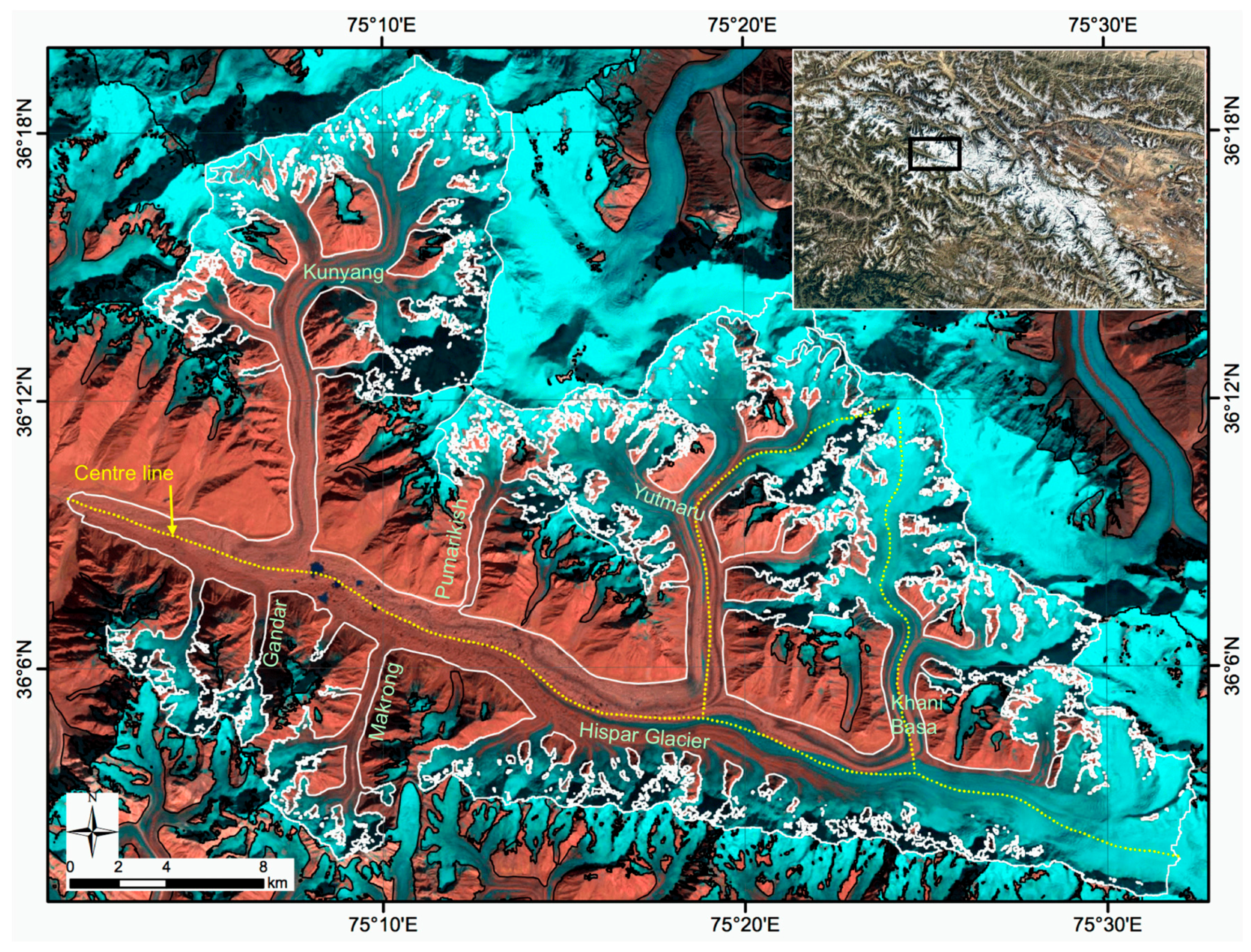
Figure 2.
Time series of the surface evolution of the lower part of Hispar Glacier as seen with the Landsat sensors (a) MSS (1977), (b) TM (1990), (c) OLI (2013), and (d) ETM+ (2015). Arrows and circles point to specific surface features discussed in the text. Image (a) is a false colour composite with MSS bands 6, 5, 4 as RGB, images (b–d) use the SWIR, NIR and red channel as RGB.
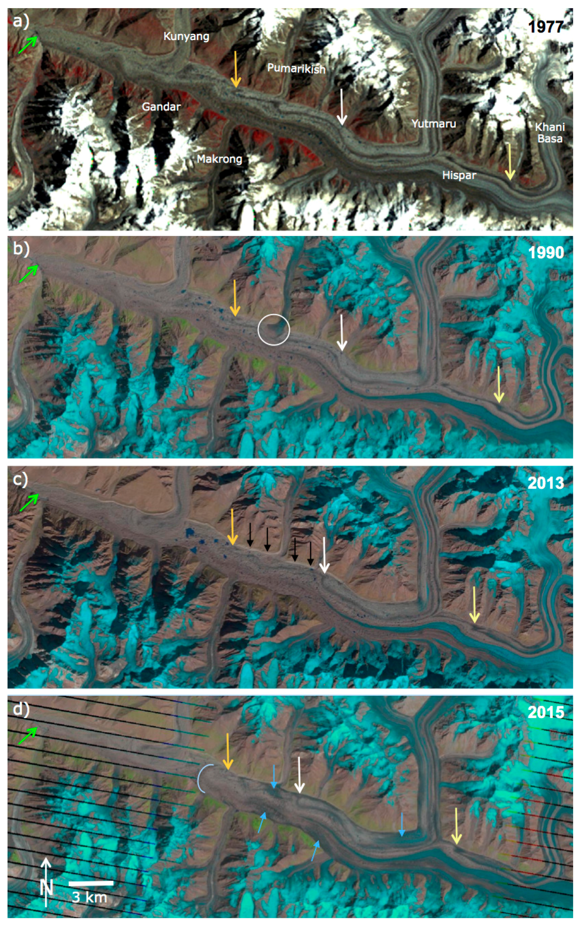
Figure 3.
Pre-surge variability of flow velocities in the summer of 2013 (a) and (b) and 2014 (c) and (d) derived from Landsat 8 OLI. (e) Initiation of the surge in late autumn 2014 by the Yutmaru tributary (red) and (f) start of the full surge in winter 2014/15. (g) is the same as (f) but with a different colour table to better reveal the further acceleration of the flow shown in (h). Coordinates are in UTM43N.

Figure 4.
Evolution of flow velocities in a time-distance plot along the flow line of HG. The black dotted line across all dates shows the position of the confluence with the Yutmaru tributary.
Figure 4.
Evolution of flow velocities in a time-distance plot along the flow line of HG. The black dotted line across all dates shows the position of the confluence with the Yutmaru tributary.
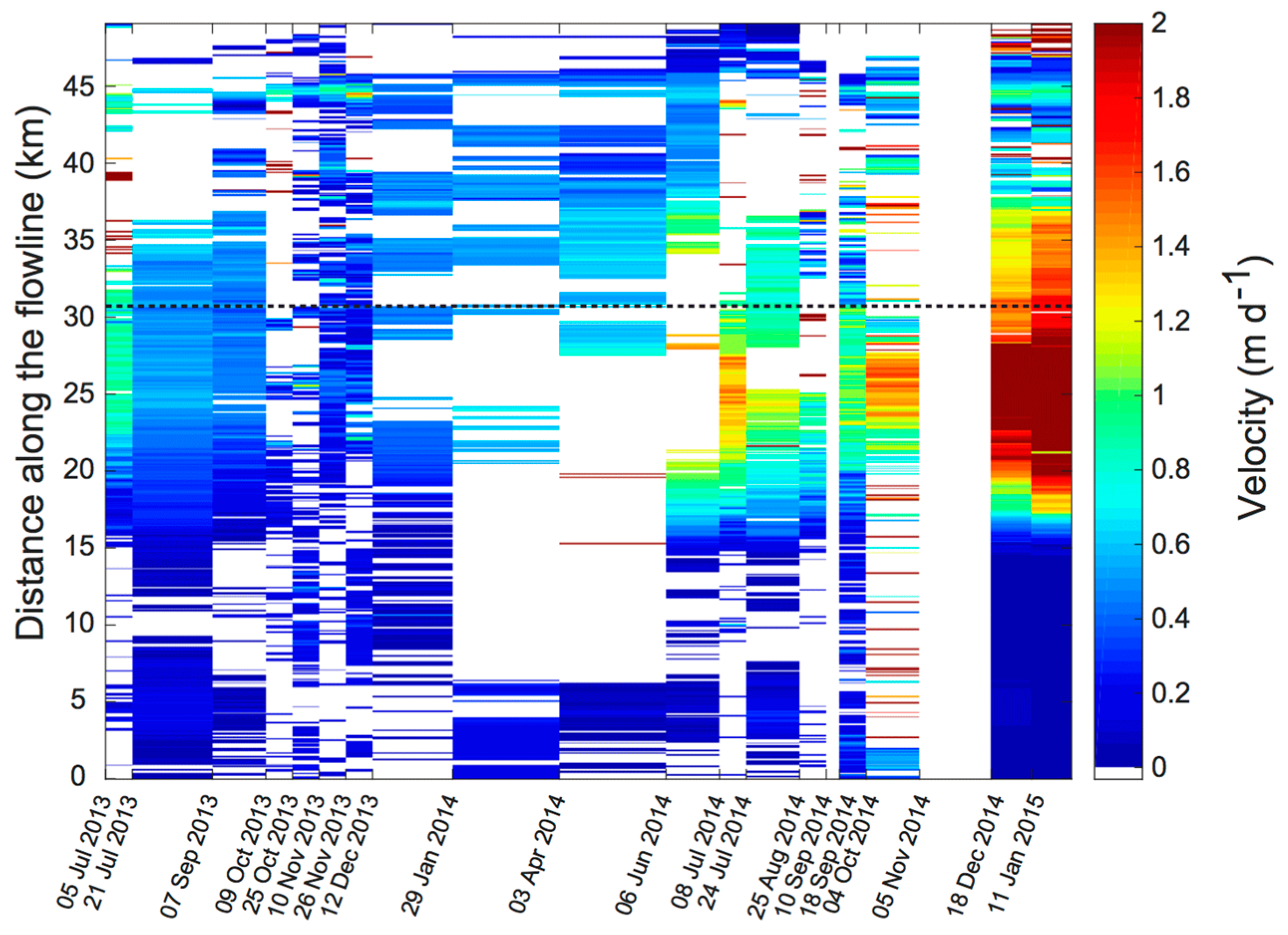
Figure 5.
(a–h) Temporal evolution of flow velocities from spring 2015 to summer 2016 derived from Sentinel-1. Highest velocities are reached by the end of May 2015 (d). After a substantial velocity decrease in autumn 2015 (f), velocities increased again in 2016 (g) and (h). Please note the different colour scale in Figure 5 (max. 15 m d−1) and Figure 6 (max. 10 m d−1).

Figure 6.
Evolution of flow velocities during the surge in a time-distance plot along the flow line of HG (cf. Figure 4). The thick black-dotted line across all dates shows the position of the confluence with the Yutmaru tributary. The two separated fast flow periods are clearly visible.
Figure 6.
Evolution of flow velocities during the surge in a time-distance plot along the flow line of HG (cf. Figure 4). The thick black-dotted line across all dates shows the position of the confluence with the Yutmaru tributary. The two separated fast flow periods are clearly visible.
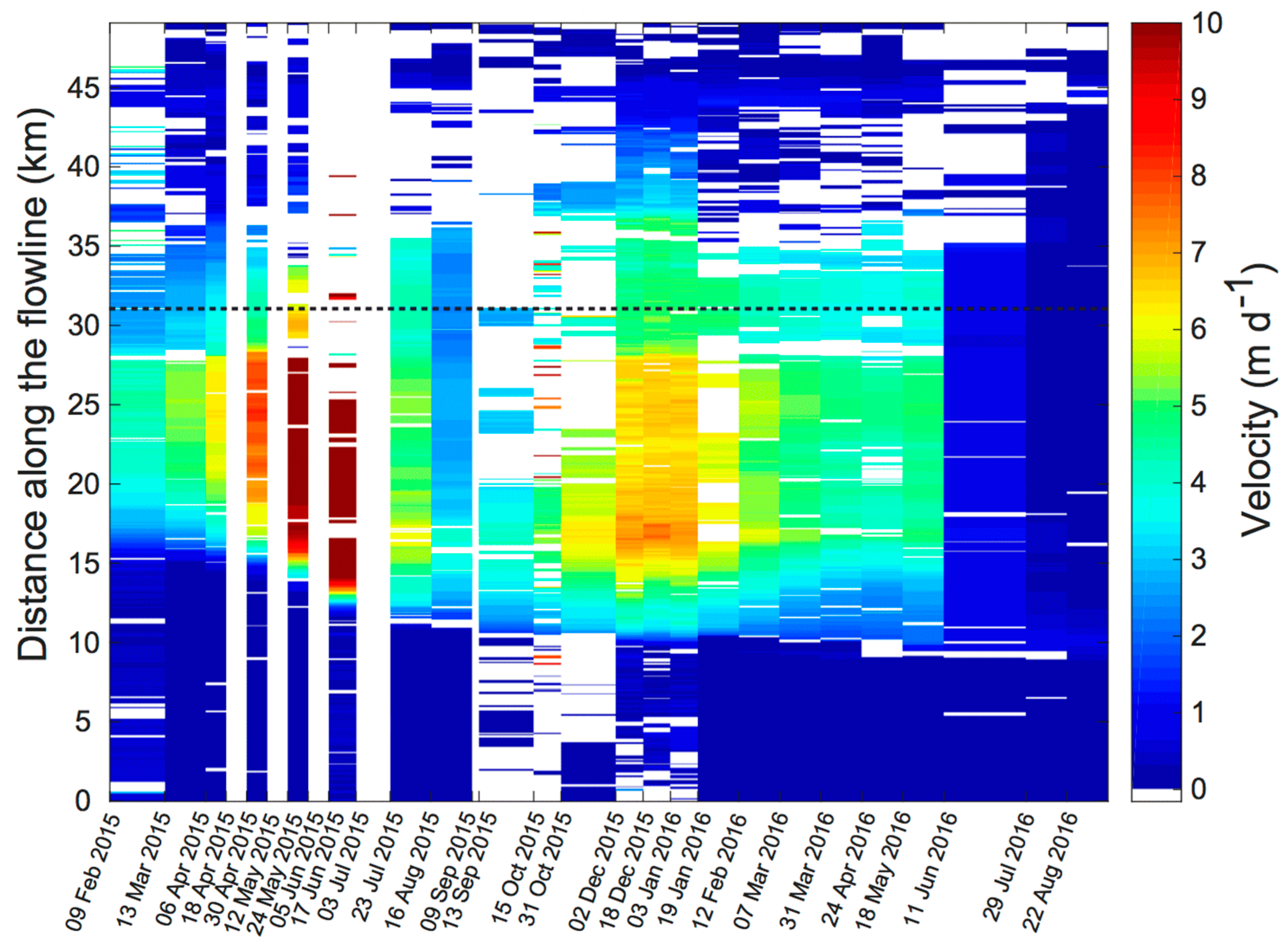
Figure 7.
Annotated time-series of flow velocities vs. distance from the terminus along the central flow line of Hispar Glacier, colour coded for date and using a 200 m sampling. The location of the two tributaries is indicated. The vertical double arrow is indicating the increase in velocity while the surge front was stable. Note: 3650 m y−1 equals a flow velocity of 10 m d−1.
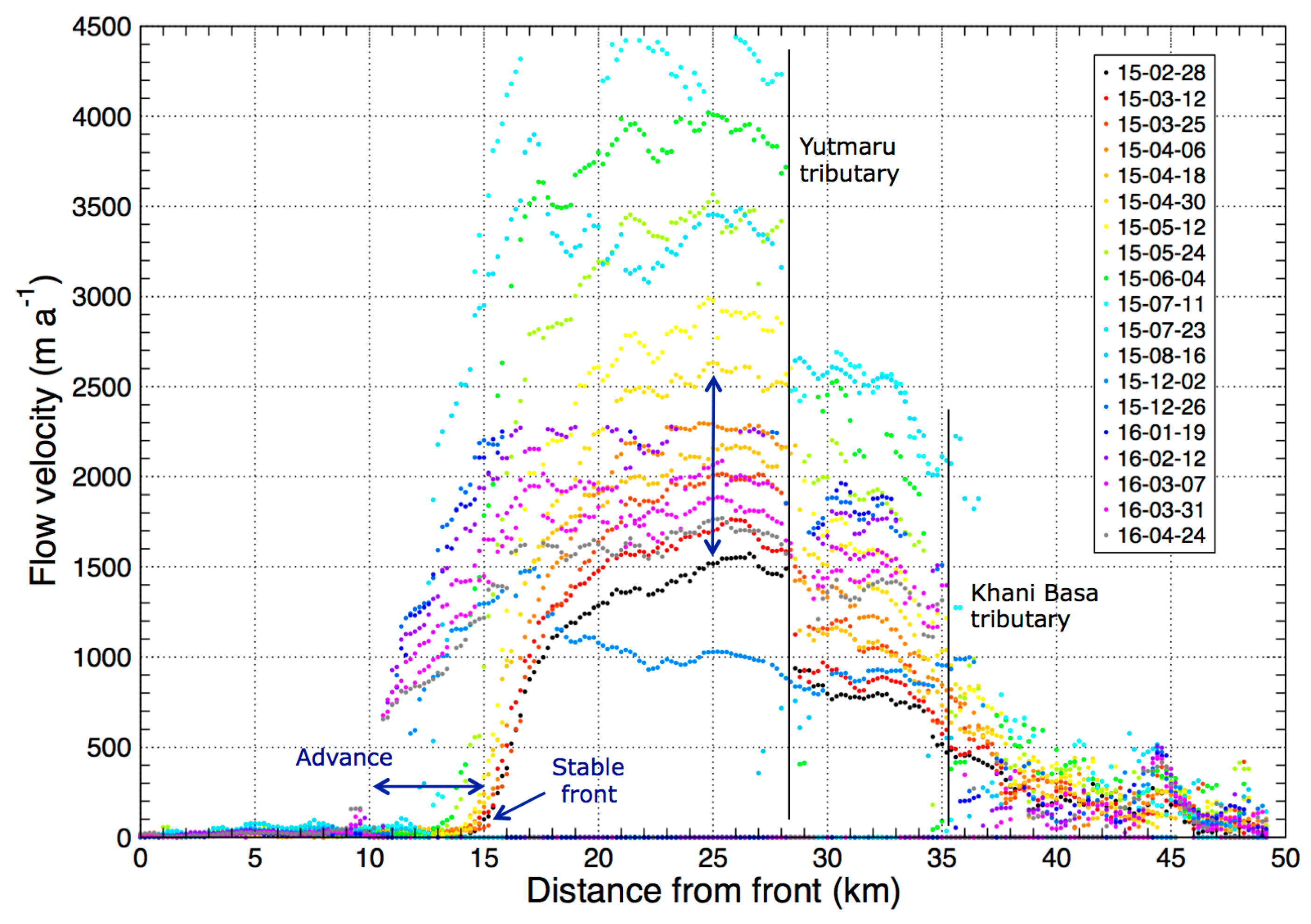
Figure 8.
Averaged flow velocities for the main glacier and its two tributaries (E: Khani Basa, W: Yutmaru) at different points in time. For the main glacier only velocities between km 10 and 28 (see Figure 7) were averaged.
Figure 8.
Averaged flow velocities for the main glacier and its two tributaries (E: Khani Basa, W: Yutmaru) at different points in time. For the main glacier only velocities between km 10 and 28 (see Figure 7) were averaged.

Figure 9.
Annotated Corona image from 1965 showing details of the previous surge. For comparison a screenshot of the same region in 2013 from Google Earth is shown in the inset.
Figure 9.
Annotated Corona image from 1965 showing details of the previous surge. For comparison a screenshot of the same region in 2013 from Google Earth is shown in the inset.

Table 1.
Specifications and processing parameters of Landsat 7 ETM+, Landsat 8 OLI, RADARSAT-2 and Sentinel-1 data. The spatial resolution of the velocity map is 100 × 100 m for all sensors.
Table 1.
Specifications and processing parameters of Landsat 7 ETM+, Landsat 8 OLI, RADARSAT-2 and Sentinel-1 data. The spatial resolution of the velocity map is 100 × 100 m for all sensors.
| Landsat ETM+ | Landsat OLI | RADARSAT-2 | Sentinel-1 | |
|---|---|---|---|---|
| Mode | Panchromatic | Panchromatic | Wide Fine | IWS |
| Scene coverage (km) | 170 × 183 | 170 × 183 | 150 × 150 | 250 |
| Pixel resolution (m) | 15 × 15 | 15 × 15 | 10.6 × 5.2 | 3 × 22 m |
| Matching window (pixel) | 15 × 15 | 15 × 15 | 38 × 77 | 256 × 128 |
| Search area (pixel) | 50 × 50 | 50 × 50 | 38 × 77 | 256 × 128 |
| Step size | 100 m | 100 m | 9 × 19 pixel | 40 × 10 |
© 2017 by the authors. Licensee MDPI, Basel, Switzerland. This article is an open access article distributed under the terms and conditions of the Creative Commons Attribution (CC BY) license (http://creativecommons.org/licenses/by/4.0/).
Share and Cite
MDPI and ACS Style
Paul, F.; Strozzi, T.; Schellenberger, T.; Kääb, A. The 2015 Surge of Hispar Glacier in the Karakoram. Remote Sens. 2017, 9, 888. https://doi.org/10.3390/rs9090888
AMA Style
Paul F, Strozzi T, Schellenberger T, Kääb A. The 2015 Surge of Hispar Glacier in the Karakoram. Remote Sensing. 2017; 9(9):888. https://doi.org/10.3390/rs9090888
Chicago/Turabian StylePaul, Frank, Tazio Strozzi, Thomas Schellenberger, and Andreas Kääb. 2017. "The 2015 Surge of Hispar Glacier in the Karakoram" Remote Sensing 9, no. 9: 888. https://doi.org/10.3390/rs9090888
Note that from the first issue of 2016, this journal uses article numbers instead of page numbers. See further details here.