Fusion of SAR, Optical Imagery and Airborne LiDAR for Surface Water Detection


1
Department of Geological Sciences and Geological Engineering, Queen’s University, Kingston K7L 3N6, ON, Canada
2
Department of Biology, Queen’s University, Kingston K7L 3N6, ON, Canada
*
Author to whom correspondence should be addressed.
Remote Sens. 2017, 9(9), 890; https://doi.org/10.3390/rs9090890
Submission received: 10 July 2017
/
Revised: 21 August 2017
/
Accepted: 22 August 2017
/
Published: 28 August 2017
(This article belongs to the Section Remote Sensing in Geology, Geomorphology and Hydrology)
Abstract
:The detection and monitoring of surface water and its extent are critical for understanding floodwater hazards. Flooding and undermining caused by surface water flow can result in damage to critical infrastructure and changes in ecosystems. Along major transportation corridors, such as railways, even small bodies of water can pose significant hazards resulting in eroded or washed out tracks. In this study, heterogeneous data from synthetic aperture radar (SAR) satellite missions, optical satellite-based imagery and airborne light detection and ranging (LiDAR) were fused for surface water detection. Each dataset was independently classified for surface water and then fused classification models of the three datasets were created. A multi-level decision tree was developed to create an optimal water mask by minimizing the differences between models originating from single datasets. Results show a water classification uncertainty of 4–9% using the final fused models compared to 17–23% uncertainty using single polarization SAR. Of note is the use of a high resolution LiDAR digital elevation model (DEM) to remove shadow and layover effects in the SAR observations, which reduces overestimation of surface water with growing vegetation. Overall, the results highlight the advantages of fusing multiple heterogeneous remote sensing techniques to detect surface water in a predominantly natural landscape.

1. Introduction
Synthetic aperture radar (SAR), light detection and ranging (LiDAR) and multispectral imaging are established remote sensing techniques for use in land cover classification models [1,2,3]. Many studies assess the ability to integrate two remote sensing techniques to detect wetlands [4,5,6,7,8,9,10,11,12]. However, fewer studies discuss the ability to integrate all three [13,14]. A number of studies assess the ability of an integrated model to detect wetlands, e.g., in [13], the focus is on prairie grasslands and LiDAR is used to correct terrain effects in the SAR models. The objectives of this study are to: (1) develop a synergistic water classification model by integrating models derived from three independent sensors, SAR, optical, and LiDAR; (2) compare the integrated models to those derived from individual remote sensing techniques; and (3) investigate discrepancies in land cover classification between the individual techniques and the integrated models, with a focus on surface water.
SAR detects differences in the dielectric and geometric properties of target surfaces, which affects the intensity of the backscatter signal. Water has a high dielectric constant and generally acts as a specular reflector, thus it is differentiable in SAR imagery appearing dark with low backscatter. Misclassification errors of omission can occur due to wind (which creates waves on the water surface), flooding of vegetated areas, or ice cover [1]. Several studies demonstrate the utility of single polarization SAR data for analyzing surface water extent and changes. SAR observations can also penetrate vegetation, to varying degrees, depending on the wavelength, vegetation type and canopy conditions. However, due to the side looking nature of SAR, some areas on the ground surface may be misclassified when terrain, urban agglomerates, or vegetation create regions of radar shadow (commission error) and layover (omission error) [15]. Regional studies including RADARSAT-1, RADARSAT-2 and TerraSAR-X (TSX) data for mapping open water can be found in [16,17,18]. For the purpose of flood mapping, single polarization SAR imagery is used to create time-series of water changes [19,20] and fully automated processing chains using TSX and ENVISAT SAR [18,21]. Processing techniques applied to SAR in order to map surface water include multi-temporal interferometric SAR coherence, active contour modeling, and texture-based classification. The most commonly used approach, also used herein, is Grey-level thresholding [1,21].
Airborne LiDAR scanning (ALS) surveys use laser pulses to collect both positional and intensity information for each reflector point [22]. Associated with each data point is an intensity value, which is a measure of the strength of the backscattered signal. This intensity value is influenced by the spectral characteristics of the material at the wavelength used by the LiDAR instrument. As an active remote sensing technique, data can be acquired during the day or night. Although surveys should be performed in cloud- and fog-free conditions, the survey can often be flown beneath the cloud ceiling for land cover classification studies. Other environmental variables, such as wind, can affect the collected data [23]. An advantage of ALS surveys is their customizability. Spatial coverage and resolution of the data can be controlled, and is mainly dependent on the height of the LiDAR platform, aircraft speed, scanning frequency and pulse repetition frequency of the instrument, and swath width [24]. The ability to record more than one return signal per emitted pulse also enables LiDAR to generate a three-dimensional model of the landscape. In temperate forests, the signal is able to penetrate through the tree canopy and provide information about the forest floor. This creates the potential for LiDAR to detect inundation below a forest canopy [25]. Water is typically characterized by: (i) having a low elevation when compared to the immediately neighboring landscape; (ii) low elevation variability; (iii) a low intensity signature at high incidence angles [25] and (iv) a high intensity signature at low scan angles [26], both related to the specular nature of calm water [27]; (v) a high incidence of laser point “dropouts” which occur when the return signal is too weak to detect [2]; and (vi) as a result of the high rate of dropouts, water bodies tend to have a lower point density [2]. Misclassifications can arise from the variability in the intensity signature which lead to portions of water bodies being misclassified as fields or similar land cover classes. Flat areas including roads and agricultural land cover that have similarly low intensity signatures can also be misclassified as water.
Much progress has been made in using LiDAR intensity data to classify land cover from the first proof of concept study performed by [28]. This study uses a pixel-based decision tree classification system which incorporates parameters derived from both the positional and intensity data to identify bodies of water [2,29]. Both intensity and positional data were used as inputs to the model to capitalize on the wealth of data provided by LiDAR surveys.
Since the launch of Landsat in 1972 [6], multispectral imagery has been the principle data type for land cover classification studies. Current multispectral satellite missions include up to eight spectral bands in the visible-to-near infrared (NIR) wavelengths, an average revisit period of 1.1 days, and a spatial resolution reaching 0.3–0.5 m [30]. Water is characterized in multispectral imagery as having a low reflectance, especially in the NIR wavelengths. For this reason, some land cover classification studies use the NIR band to separate water from land [31]; others use band ratios to extract water bodies [32,33,34] and supervised classification techniques [35]. However, these techniques can be confounded by shadows, which can be misclassified as water [36,37,38]. Optical imaging is unable to penetrate vegetative cover, which results in challenges with detecting areas of inundation below forest canopies. While some of these limitations may affect the ability of optical imagery to correctly classify all bodies of water, in a cloud-free scene optical imagery has proved to classify open bodies of water successfully.
In this study, TSX scenes were combined with airborne LiDAR and optical imagery using a pixel based decision tree analysis to classify areas of water and non-water and identify areas where the classification was uncertain. TSX has a repeat period of 11 days and a resolution of up to 0.24 m in staring spotlight beam mode [39,40], allowing for frequent monitoring of small water bodies. The methodology, processing techniques and decision tree analysis used to exploit the strengths of each sensor are described in the following sections. The fused water models are visualized, analyzed and compared to the single sensor models in order to identify discrepancies. Ultimately, the percent of water and uncertainty of each model is determined in order to understand the influence of using multiple data sets to classify surface water.
2. Materials and Methods
2.1. Study Area and Data Description
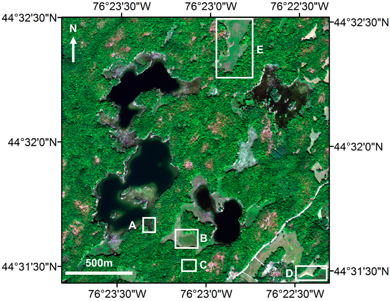
The study area is located at the Queen’s University Biological Station (QUBS) in Kingston, Ontario, Canada, approximately 50 km north of the eastern end of Lake Ontario. QUBS was chosen due to the abundance of water bodies that vary in size from small inundated forests to large open bodies of water. The 2 km × 2 km square area where the SAR, LiDAR and optical data sets overlap is shown in Figure 1.
Five TSX staring spotlight mode scenes were acquired over QUBS from April to September 2016. These scenes represent single look slant range (SSC) products of descending path, single polarization (HH), right looking with an incidence angle of 44°. They have a slant range and azimuth resolution of up to 0.6 m and 0.24 m, respectively. The LiDAR data were acquired using an Optech Gemini ALTM, which is a small-footprint, single wavelength, discrete return system. The survey was flown in June 2015 at an altitude of 1200 m, and resulted in a spatial resolution of 1 pt/m2. WorldView-2 imagery was acquired in August 2016 consisting of 8-band multispectral optical images with a resolution of 2 m. Table 1 outlines the data sets used in this study.
In situ field investigations were performed on three different occasions, which overlap with three of the five SAR acquisition dates. During these field investigations to five chosen study locations, GPS coordinates were recorded as well as water and site conditions, including the presence of open water, flooded vegetation, and the dominant vegetation type such as reeds, shrubs or forest. The five sites were chosen for having different environmental and surface water conditions as follows:
- Poole Lake: A large, open body of water bordered by wetlands and mixed forest.
- Marsh A: A dense cattail marsh connected to a small lake, with the potential to be flooded during parts of the year. A small stream runs along the periphery of the marsh.
- Inundated Forest: A small area of observed inundation beneath a mixed forest canopy with some emergent shrubbery. Depth of water in April was approximately 1 m.
- Marsh B: A small pond bordered by a sparse cattail marsh, which immediately backs onto a flat field to one side and a forest to the other side. The forested side is beyond the chosen study area. Water level was observed to be highest in the spring and receded throughout summer.
- Vegetated Lake: A wetland composed of a central pond/marsh, transitioning into a dense cattail marsh along the periphery. In the central pond/marsh, there are sparse cattails and the remnant trucks of dead trees. A central stream cuts through the marsh, connected to peripheral streams throughout the marsh.
The locations of these sub-areas are shown in Figure 2.
2.2. SAR Processing
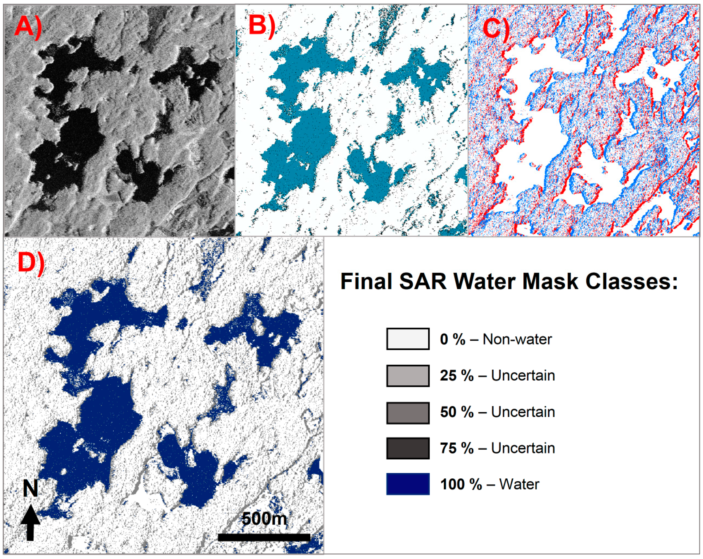
The single-polarization TSX staring spotlight mode scenes were processed to create five SAR water masks that each contain five different classes. The TSX intensity data were calibrated and speckle filtered using a Refined Lee 7 × 7 speckle filter three times to optimally reduce speckle while maintaining edges and histogram form [41]. A Range-Doppler Terrain correction was applied to geometrically correct the TSX data using STRM DEM [42], producing a processed SAR intensity image (Figure 3A).
Grey-level thresholding was used to classify the image into water, uncertain and non-water. This technique classifies all pixels with a value less than this threshold as water. The histogram of the backscatter intensity data from each SAR scene was used to calculate the threshold values. The histogram is bimodal, with one mode largely representing water and the other representing dry land. The local minimum between the two modes represents the area of transition between water and non-water. Two thresholds were chosen which could separate classes of water and uncertain, and uncertain and non-water. Three normal distribution curves were fit to the histogram data. Since the left mode (representing water) was skewed to the left, two normal distribution curves were fit to this, one using the variance and one using the mean. Where these two curves intersected with the right mode’s normal distribution fitted curve represents the two threshold values. Intensity values in-between the two thresholds were marked as the class “uncertain”. Values greater than the thresholds were classified as “non-water” and values less than were classified as “water”. Figure 3B displays the SAR threshold water mask.
The next step in SAR processing involved determining the shadow and layover zones, which exist in the SAR scenes and can confound classification using intensity values [15]. Areas of shadow occur where the radar wave is blocked from reaching the ground surface. This creates areas of false positives for water (error of commission). Layover zones occur where the returns from two surfaces with equal distances to the sensor are received simultaneously, creating errors of omission. The approach to shadow and layover zones used in this study were adapted from Mason et al. (2010). This includes the traditional shadow and layover zones created by terrain geometry, but also includes occluded areas caused by tall vegetation [15]. Due to the varying degrees of canopy (density, canopy closure, growth state, and tree type) throughout the SAR scenes, and signal attenuations from leaves, the assumption is made that the tree canopy is impenetrable, similar to urban infrastructure and terrain. Therefore, a shadow and layover mask was generated using the satellites geometric parameters (incidence angle and azimuth) and a LiDAR digital elevation model (DEM), combining the affects from both the terrain elevation and vegetation height. It is noted that, if LiDAR surveys are conducted in concert with the SAR scenes, further vegetative parameters such as density derived from the intensity and positional data from the surveys can be used to further refine the shadow and layover mask. However, due to the disparate acquisition dates of these data, and the seasonality of vegetation cover in the study area, only the parameter of vegetation height, integrated in the DEM, was considered. Figure 3C shows the error mask delineated into three classes: shadow region (blue), layover region (red), and no error (white).
Finally, the SAR classified water mask and the error mask were combined to create a final SAR water mask for five different classes with each class representing the estimated probability that the pixel is water. The estimated probability values were assigned as 0, 25, 50, 75 and 100 to represent the five different classes evenly distributed between 0% and 100%. Figure 4 outlines the decision tree used to classify each pixel in the SAR model. For instance, pixels in the uncertain zone between thresholds that were also within a shadow error of commission zone were assigned a probability of 25% water (highlighted in Figure 4). Five final SAR water masks were created; one for each acquisition date. Figure 3D shows the final SAR water mask for the 2 April 2016 TSX acquisition.
2.3. LiDAR Processing
As noted in Table 1, airborne LiDAR data were acquired over QUBS in June 2016 using an Optech Gemini ALTM, which is a small footprint, discrete return LiDAR instrument capable of recording 4 return pulses per emitted pulse, each with an associated intensity value. The LiDAR data provided was filtered for outliers and ground classified. The original point cloud was rasterized into 3 m × 3 m pixels for further processing. Rasterization was performed for each input parameter individually. A tiered decision tree classifier (adapted after [29]), was used to classify water in the study area using both the positional and intensity data available in the LiDAR dataset.
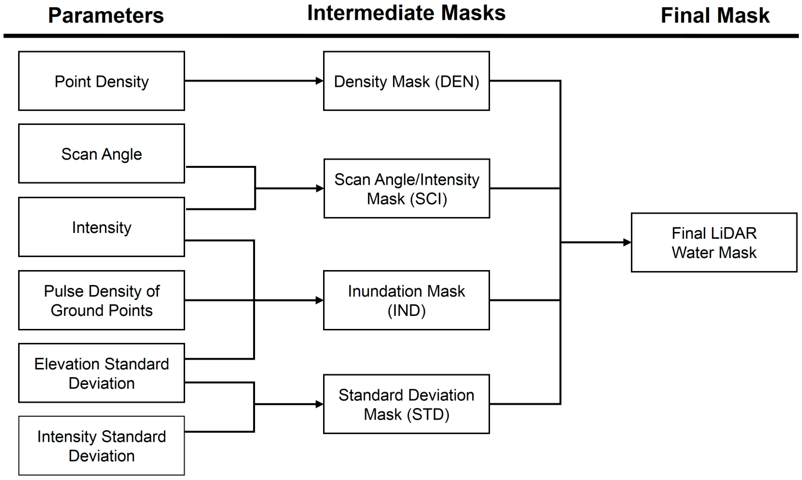
The six input parameters used for this study are: (1) point density; (2) intensity; (3) scan angle; (4) standard deviation of intensity; (5) standard deviation of elevation; and (6) pulse density of only ground classified points; these parameters are illustrated in Figure 5. Subsets of these parameters were combined into four intermediate water masks as illustrated in Figure 6:
- The Density Mask (Mask DEN) was generated using only point density; due to the specular reflection of water, open bodies of water have a high rate of point dropouts and thus a low point density [2]. This is contrasted with forested areas which commonly have more than one return signal per emitted signal, and open fields which do not generally produce point dropouts.
- The Scan Angle/Intensity Mask (Mask SCI) was generated using scan angle and intensity data; because of its properties as a specular reflector, open water bodies typically have low intensity at high incidence angles and high intensity beneath the nadir of the platform and at smaller incidence angles.
- The Standard Deviation Mask (Mask STD) incorporates the standard deviations of intensity and elevation; open bodies of water are by definition flat, and so have a low variation in elevation. They are also characterized as having a low standard deviation of intensity at moderate scan angles because of the consistent reflection of the laser signal away from the receiver and subsequent low intensity returns and dropouts, and a high standard deviation of intensity at low scan angles because of the contrasting high intensity returns beneath the nadir of the plane and low intensity returns from the neighboring flight strips due to the effects of flight strip overlap [2,29].
- The Inundation Mask (Mask IND) was generated to highlight forested areas that have the potential to be inundated and was generated by integrating the pulse density of ground points, elevation standard deviation, and intensity; this mask was made by visually inspecting the raster of each individual parameter to identify patters in the study area. A region of moderately low intensity within a forested area was noted. The low intensity could be indicative of water cover beneath the forest canopy, which would lower the average intensity of the returns from that area. Pulse density was used to identify areas where the LiDAR signal was routinely able to penetrate the forest canopy and correctly classify ground points. A forest which is flooded for a significant portion of the year is likely to be unhealthier than the surrounding forest, allowing more laser pulses to reach the ground surface beneath the canopy [43].
Finally, once the inundated forest model was created, it was checked visually against optical imagery of the area and a DEM created from the LiDAR data. Visual inspection of the optical imagery did not reveal any indication of the forest being flooded. However, on inspection of the DEM it was observed that the area of inundation is flat, occurs in a local elevation minima, and most notably it appears to connect the lakes in the study area with Lake Opinicon, a larger lake east of the study area. Along with connecting those water bodies, the elevation of the area suspected of inundation is intermediate between that of the lakes in the study area and Lake Opinicon.
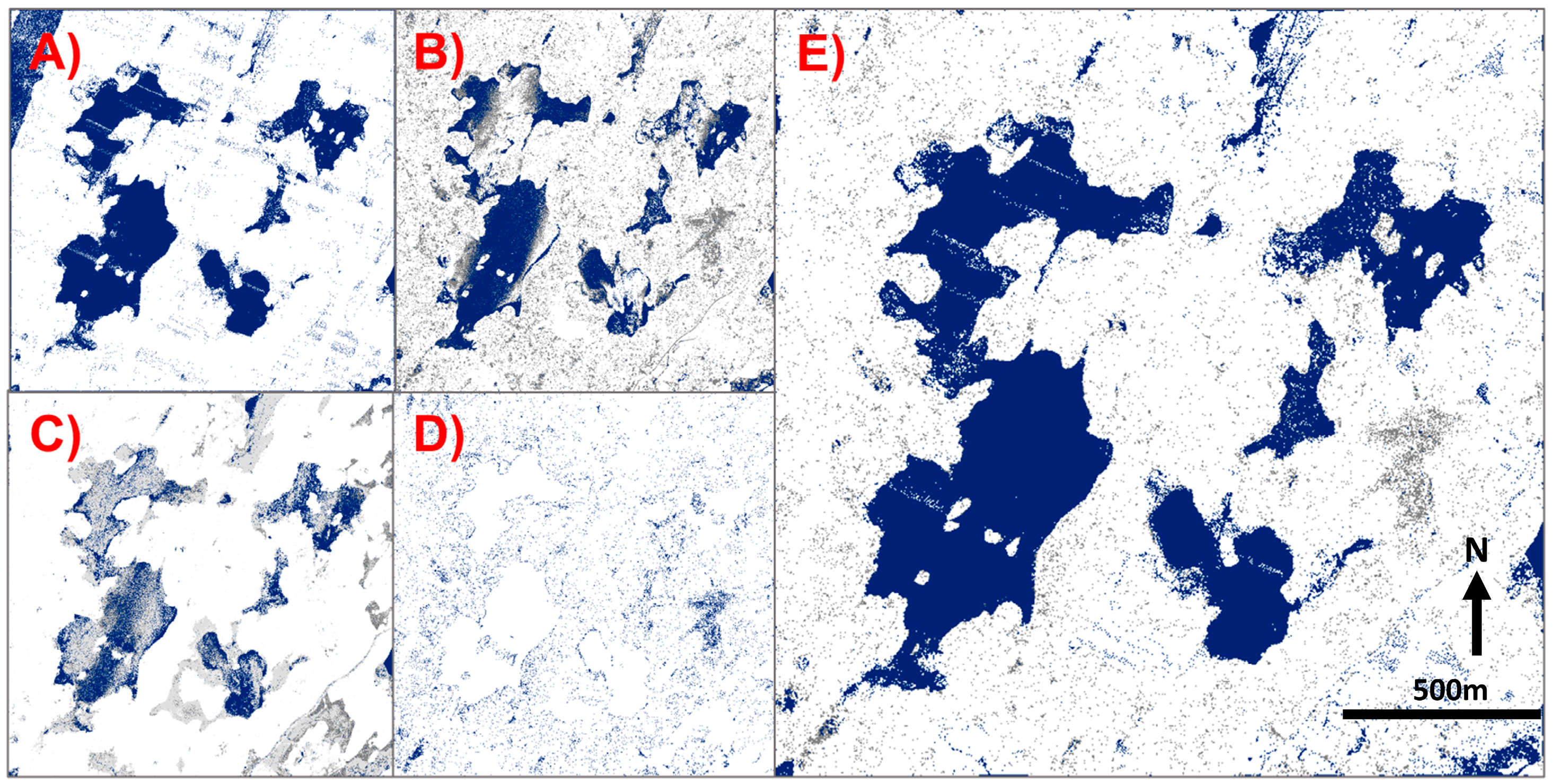
The final water mask was generated through a decision tree using each of the intermediate water masks as inputs (Figure 7). Because water does not have one distinctive elevation, intensity, or point density signature, each of the intermediate water masks was developed to isolate one or more sections of the water body. Each of the masks was optimized to minimize noise and errors of commission (false positives). Therefore, when generating the final water mask, a pixel was classified as 100% water if either the SCI mask or the STD mask classified it as water. Due to artifacts introduced into the density mask from the variations in airplane orientation throughout the flight, and through a miscalculation in flight trajectory, the density mask could not be directly input into the final mask. Instead, the DEN mask was filtered to only classify pixels as water if they had both a low standard deviation of elevation and had a low point density. Pixels that were identified as being potentially inundated were assigned a value of 50% in the final LiDAR water mask.
2.4. Optical Imagery Processing
WorldView-2 8-band multispectral imagery was used to create a water mask using the Normalized Difference Water Index (NDWI) and the Normalized Difference Vegetation Index (NDVI) seen in Equations (1) and (2), respectively.
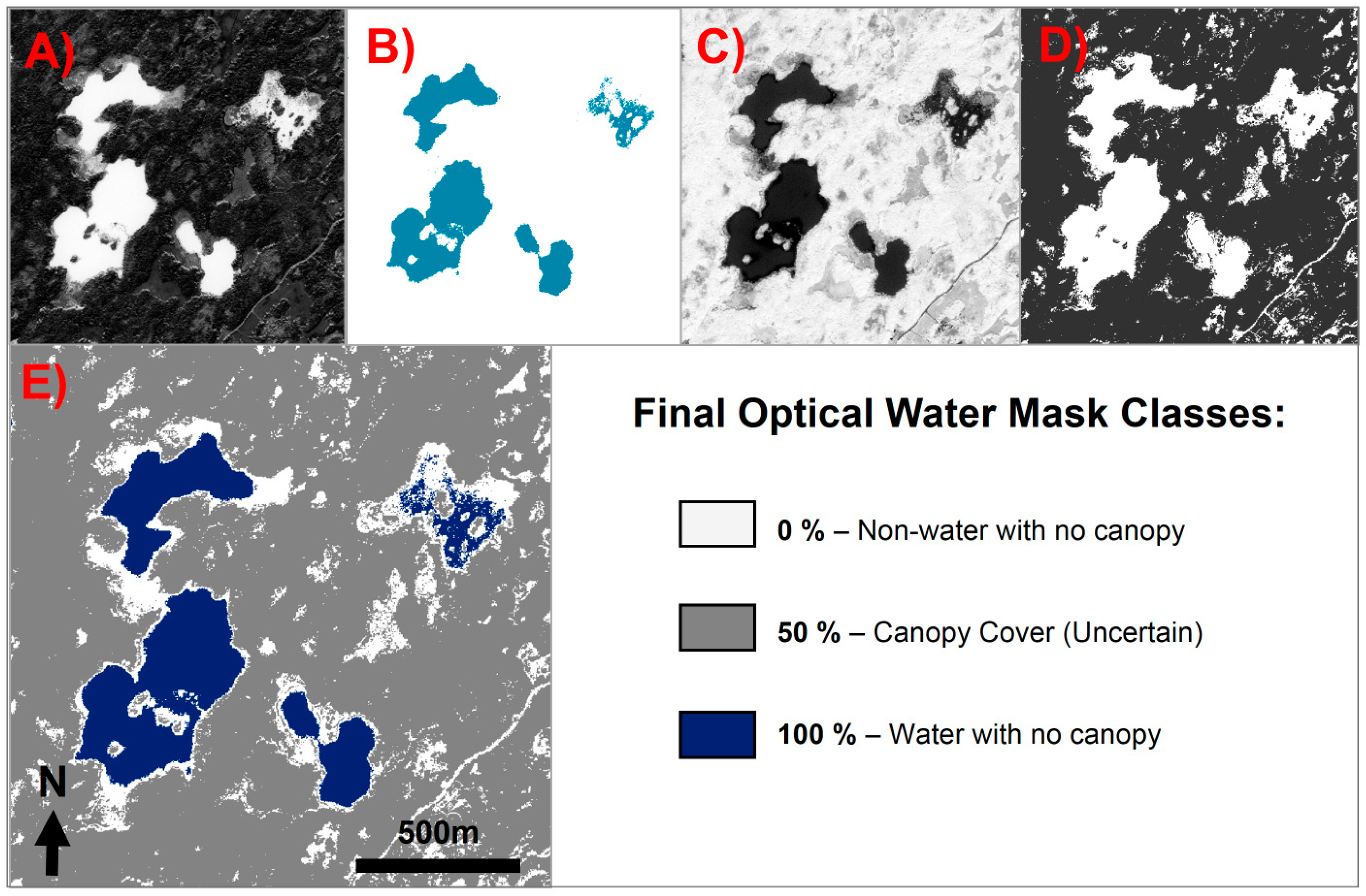
These equations utilize the coastal and NIR2 bands unique to WorldView-2, which provide a larger difference in wavelength, resulting in a more discrete threshold for detecting water and vegetation [30,44,45]. The NDWI is used to identify areas of water, which is characterized by high values, since the coastal band maximized the reflectance of water and the NIR2 band minimizes the reflectance of water (Figure 8A). The NDVI is used to identify vegetation, where higher values characterize healthier growth (Figure 8C). The red band is traditionally used as it is absorbed by chlorophyll in healthy plant materials, and again the NIR2 band is used, as it is strongly absorbed by water and reflected by terrestrial vegetation and soil [32,44,46,47]. The histograms of both the NDWI and the NDVI are bimodal and range from −1 to +1, where the higher value mode represents water and healthy vegetation, respectively. A threshold value was chosen to segment the indices into two classes by fitting a normal distribution curve to the mode and choosing the value where the slope of the mode becomes zero. The threshold for the NDWI was 0.58, where pixels greater than the threshold were classified as water, and pixels below were marked as non-water (Figure 8B). The NDVI was used to create an error mask, where a threshold of 0.54 was used to classify areas of canopy (above) and areas of non-canopy (below). This error mask represents the areas where the signal from optical remote sensing would be obstructed and water on the ground surface under vegetation could not be detected (Figure 8D).
Finally, the optical water mask and the optical error mask were combined to create a final optical water mask with three classes. Pixels were assigned a probability of that pixel being water. Areas where non-water was classified and where no tree canopy exists were marked as 0% probability water. Pixels within the error zone were assigned a 50% probability of being water due to the inability of the instrumentation to correctly classify land cover type beneath the canopy. The remaining pixels, representing where water was classified with no error, were given a value of 100% water. The final optical water mask can be seen in Figure 8E.
2.5. Fused Water Model
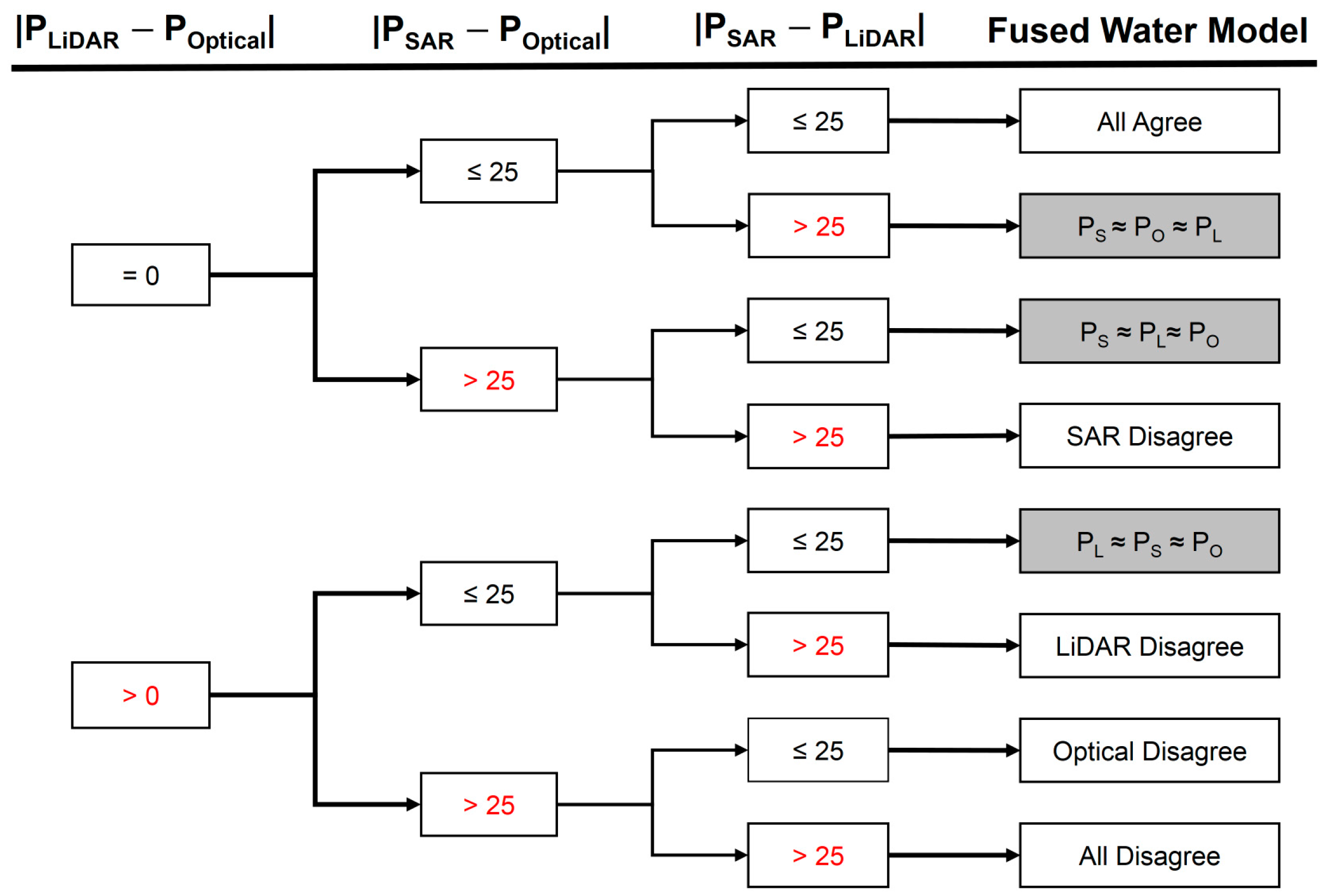
The final water masks created from all three datasets result in a fused water model that exploits the strengths and compensate for the weaknesses of SAR, airborne LiDAR and optical imagery. Since there were five different SAR acquisitions and water masks, each of these was combined with LiDAR and optical to create five different fused water models, each representing a different point in time. This fused model classifies pixels based on the agreement of the sensors at each pixel. As a measure of agreement, each of the masks generated from the different remote sensing techniques were differenced from each other. The absolute values of these differences were used in a decision tree analysis (Figure 9) to determine the value of the pixel in the final fused water model.
In the decision tree classifier, if the absolute difference between two sensors exceeded 25%, then the sensors did not agree on their classifications; for example, one sensor classified water and the other sensor did not. If the absolute difference between two sensors was less than 25%, the two sensors agreed and classified the pixel similarly (e.g., both sensors classified water). The value of 25% was chose, n as it is the difference between classes in the individual water masks. Using this principle, there were eight different possible outcomes, of which five occurred. If all sensors agreed (all differences were less than 25%), then the median values of the pixels were used in the fused water model. Similarly, if all sensors disagreed (all differences were greater than 25%), then the median values of the pixels were used. Finally, if only a single sensor disagreed, then the mask generated from that sensor was disregarded and the average of the two remaining sensors was used. When a shadow or layover zone in SAR overlapped with the tree canopy in the optical mask, both the optical and SAR were within an error zone. In this case, the LiDAR mask was used for classification in the final fused water model since it would be the most reliable sensor in that situation.
3. Results
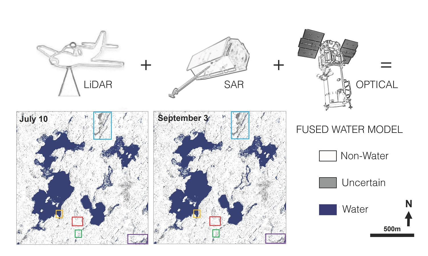
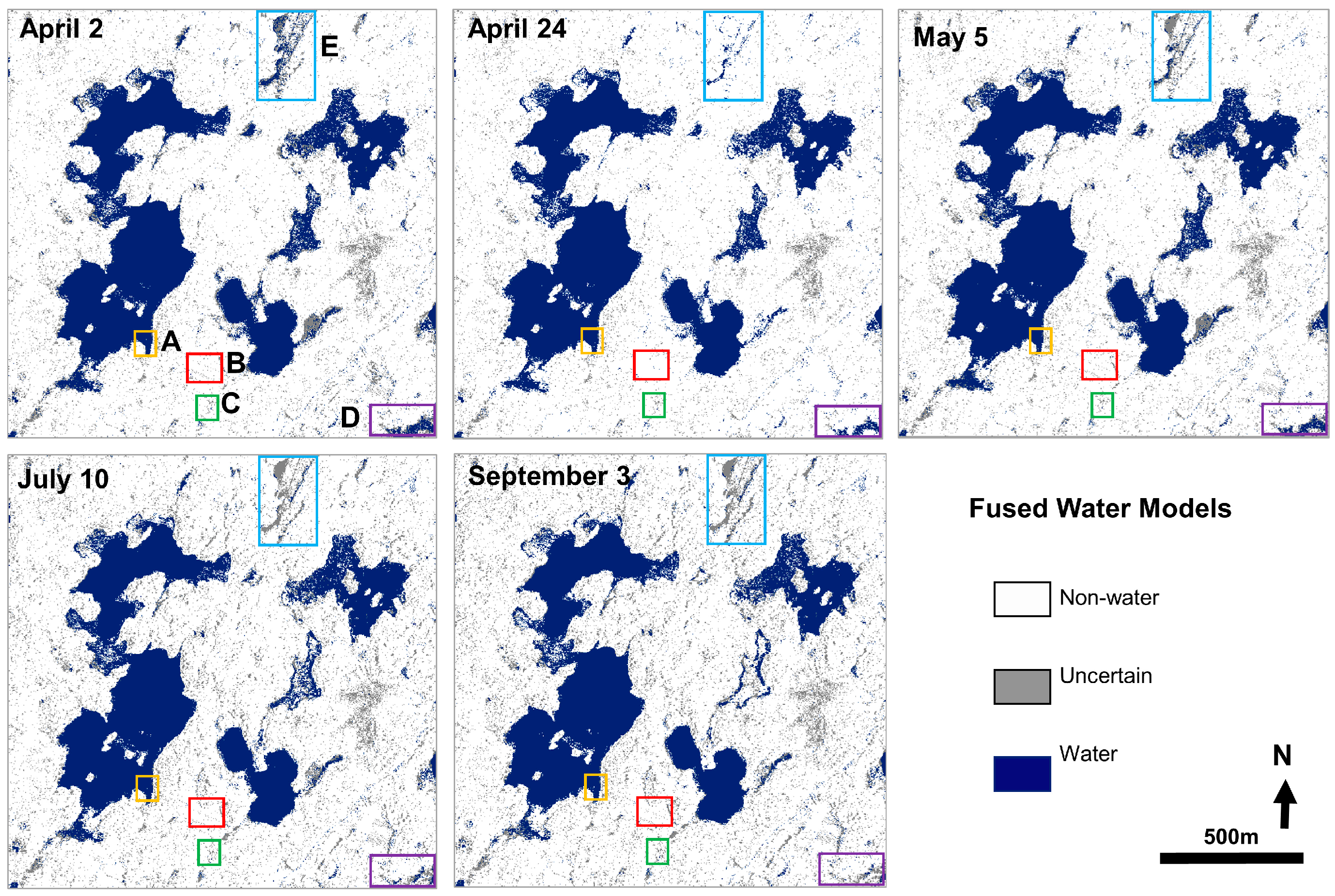
A fused model was developed by exploiting the strengths of three unique remote sensing techniques. Five different fused water models were created, representing the timeline during which the SAR scenes were acquired. These five models can be seen in Figure 10. Pixels shown in blue represent water, gray represents uncertain areas, and white pixels show non-water.
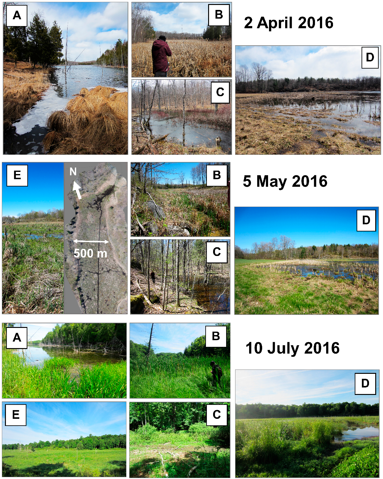
Photographs from the in situ field investigations in April, May and July 2016 can be seen in Figure 11. Observations made from the three field investigations were used to correlate the temporal changes in the fused models to seasonal changes. Seasonal changes from spring to summer in the study area are representative for a mid-continental climate and characterized by increasing temperature and vegetation cover, a decrease in precipitation, and a consequent recession of shorelines.
All five monitored locations observed a decrease in surface water extent from April to July. From April through May to July, the tree canopy was observed to be bare, budding, and in full bloom, respectively. Throughout the study area, the number of uncertain pixels in the fused models increases from 6 to 9% from April to September. The percent of water classified in the fused models is seen to decrease from 18 to 17% from April to September. Specifically, Poole Lake remained relatively unchanged throughout the season since it is a relatively large, deep body of water with steep shorelines (Yellow box in Figure 10). Similarly, water levels at Marsh A remained low throughout the season, although in some areas the mud was observed to be wet (Red box in Figure 10). The classification of Inundated Forest is also unchanged throughout the season (Green box in Figure 10), although this is because of the fact that LiDAR was only captured once for the study area, and in areas which are both covered by canopy and in shadow, the fused model defers to the LiDAR model. Marsh B receded through time with the shoreline transitioning from muddy and wet to hard and dry, a recession which is also seen in the fused models (Purple box in Figure 10). The Vegetated Lake also becomes drier through time which is observed in the field investigations and in the fused models (Blue box in Figure 10).
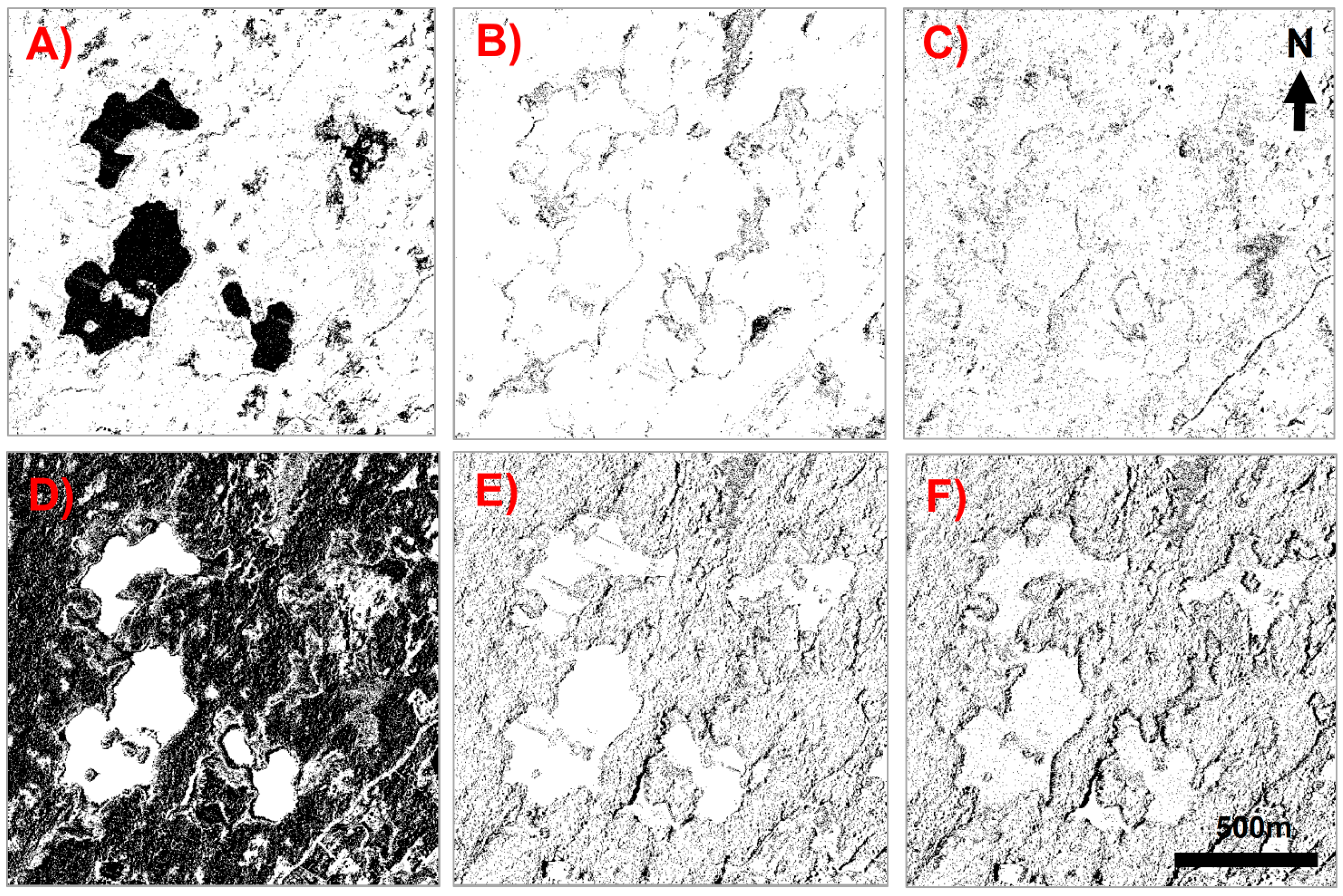
Figure 12 and Figure 13 represent each of the five outcomes of the decision tree classifier, as well as the areas where the conditional LiDAR mask was applied when both optical and SAR are in shadow. These figures highlight the areas over which each of the outcomes occur, indicating whether all sensors agree, all sensors disagree, and where either SAR or LiDAR or optical disagree with the other two techniques. Figure 12 shows the sensor agreement models for the first acquisition date (April 2016) and Figure 13 shows the sensor agreement models for the last acquisition date (September 2016). In each of these models, the black pixels represent the areas in which the labeled outcome occurred and the white areas represent where it did not.
All sensors agreed in areas with open bodies of water and fields. Disagreement was most common along shorelines, shallow bodies of water and over wetlands, i.e. areas that experience the most seasonal change. Areas over which the SAR classification disagreed, but LiDAR and optical agreed were concentrated around shorelines and within shadow and layover zones. Optical disagreed under tree cover, over flooded vegetation and over the wetlands surrounding Poole Lake. LiDAR disagreed in a few areas where classification of water was confounded by a systematic error introduced by the swaying of the aircraft during data acquisition, compounded with the variable intensity signature of water.
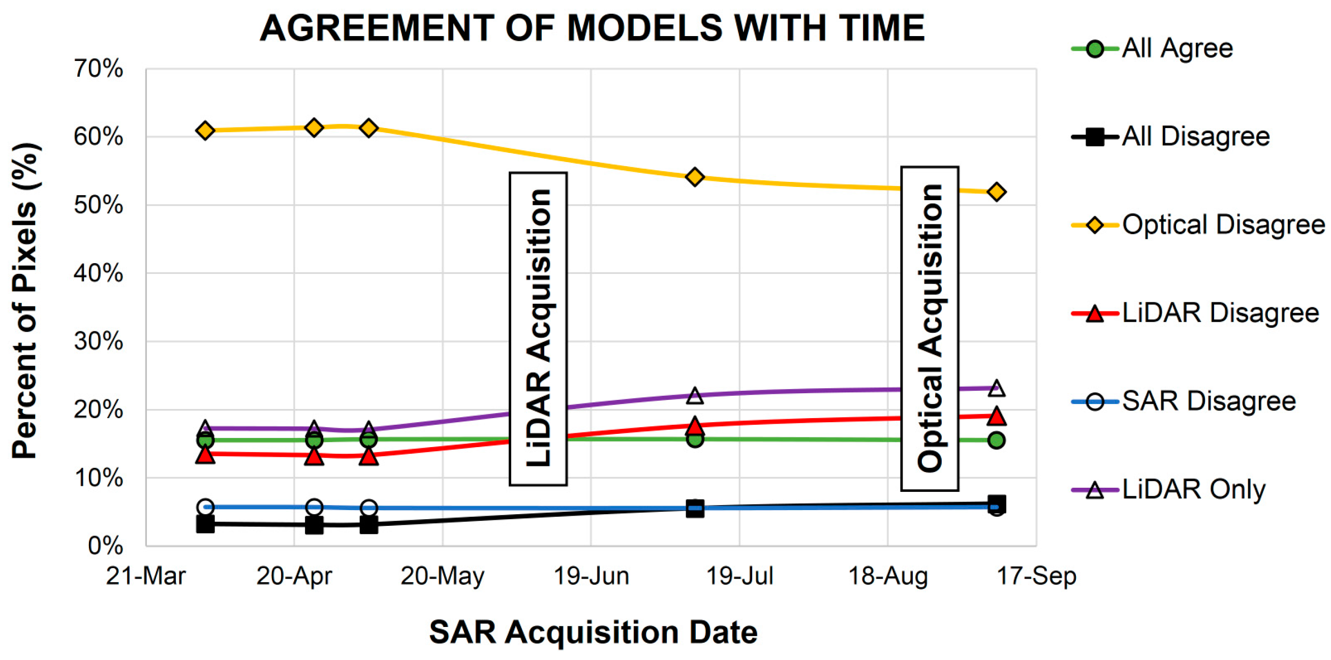
The graph in Figure 14 displays the percent of pixels of the five different outcomes and LiDAR only areas from the sensor agreement models plotted through time. Several trends were noticed. The areas where all sensors agree, mainly open water bodies and fields, remains stable through time; this is expected because these areas experience little to no seasonal fluctuation in water extent. Pixels at which all sensors disagree, principally along shorelines and over wetlands, increase through time which relates to the increase in tree canopy causing a shadow and layover error. Optical disagreement lessens while LiDAR disagreement increases and SAR disagreement remains stable. Finally, LiDAR only increases as the number of commission error of water increases from the growing tree canopy throughout the season.
Table 2 outlines the percentages of water, uncertainty, and non-water comparing each of the input water masks from the individual remote sensing techniques, and the five fused models. By fusing the three sensors together, the uncertainty within the individual SAR models was decreased from 17–23% to 4–9%. The uncertainty in the optical data was originally 75%, but, by combining with LiDAR and SAR, the uncertainty in the fused models is reduced. Although the single LiDAR model uncertainty was 4%, which is lower than the fused models uncertainty, the artifacts in the LiDAR model (such as the incorrectly identified strips over open bodies of water) were corrected for by combining the SAR and optical with the LiDAR.
4. Discussion of Results
The fused classification models indicate a decline in the extent of surface water throughout the study period, which is consistent with seasonal changes observed during field investigations. However, the uncertainty rate also increases, which could be due to the increase in tree canopy through the season, causing an increase in false positives for water, an interpretation which is corroborated by the field investigations. This ability of the fused models to correctly interpret seasonal trends in water extent fluctuations highlights its applicability for flood hazard monitoring. The models also worked over wetlands and water bodies of various depths and types of flooded vegetation.
The disagreement of the individual remote sensing techniques over wetlands and at the shorelines of larger water bodies highlights the weaknesses of each technique and the advantage of integrating SAR, LiDAR and optical remote sensing into a fused water classification model. Considering that wetlands are important indicators for flooding events and water extent change, they are one of the most relevant areas when planning a flood monitoring strategy. While the SAR only models disagreed largely in zones of shadow or layover, the disagreement of the optical models along the edge of Poole Lake may be due to those areas being shallow or having a thin vegetation cover. The ability of LiDAR to penetrate tree canopy further improves this model by being able to identify potential areas of inundated forests, and the artifacts introduced from flight conditions during data acquisition can be corrected by SAR and optical data. When comparing the spatial extent of the sensor agreement models from April (Figure 12) to September (Figure 13), the main changes seen are due to seasonal variations in the models and are located in areas where there are significant fluctuations in surface water extent due to shallow water bodies and wetlands.
The agreement between sensors over the course of the study period can mostly be explained by the dissimilar seasons in which each of the remote sensing data was acquired (Figure 14). Since LiDAR was acquired in June, LiDAR disagreement increases as it diverges from its June acquisition date. Similarly, Optical disagreement decreases as the study period progresses and converges upon its August acquisition date. SAR disagreement remains stable which is expected due to the increasing disagreement with LiDAR, but increasing agreement with optical. While temporal disagreements between sensors could be mitigated by acquiring all remote sensing data coincidently, this study demonstrates that it is not necessary for all data to be collected concurrently in order to exploit their synergies and integrate these data into a fused water extent model. This is important to note, as most remote sensing projects will not have access to all three remote sensing observation types acquired at the same time.
Ultimately, the fused model benefitted from all individual sensor and their synergies. The increase in water from 19 to 20% through time seen in the individual SAR scenes does not correlate to seasonal effects that were observed at the individual study sites, which were characterized by a progressive recession of the shallow water bodies. This increase in classifying water pixels in the SAR masks is theorized to correspond to the increase in tree canopy cover which would increase the number and extent of shadow zones, which can be misclassified as water. In the fused models, percentage of classified water decreases from 18 to 17%, which is not statistically significant.
5. Conclusions
In this study, TSX scenes were combined with airborne LiDAR and optical images using a pixel based decision tree analysis to classify areas of water and non-water and identify areas where the classification remains uncertain. This fusion technique exploits the strengths and weaknesses of each sensor and allows for an optimized fused water extent classifier which decreases the uncertainty. It was found that although the optical, SAR and LiDAR data were collected in different seasons, the uncertainty of the fused model was lower than the uncertainty of any single technique. The uncertainty in the final fused models was between 4% and 9%, compared to 17–23% from the single polarization SAR classified water models. The development of a SAR only time series of water coverage is hindered by processes including vegetation growth (leading to different errors of commission due to shadow and omission due to layover zones over time) and land cover changes which change the backscatter (and threshold per scene). Optical and LiDAR data can enhance a time series by removing some of these competing processes. In addition, the water model could be enhanced by using multi-polarization SAR to better classify areas of different scattering mechanisms, including flooded vegetation. A monitoring strategy for surface water thus needs to analyze the spatio-temporal processes of land cover change first, and then design an acquisition plan which includes optical and LiDAR acquisitions and continuous SAR acquisitions. The benefit of having access to three independent observation types was demonstrated herein, and will be used to create a flooding hazard monitoring strategy in the future.
Acknowledgments
Stephen Lougheed from the Queen’s University Biological Station (QUBS) is thanked for providing access to available data and the field site. The German Space Agency (DLR) is acknowledged for providing the TerraSAR-X data and Pacific Geomatics Ltd. for providing the WorldView-2 high resolution optical images. NSERC is also acknowledged for partially funding this research.
Author Contributions
For Katherine Irwin performed the SAR and optical data processing, developed the fused model, analyzed the data and wrote the paper. Danielle Beaulne performed the LiDAR data processing and aided in writing the paper. The field investigations were performed by Katherine Irwin, Danielle Beaulne and Alexander Braun. Alexander Braun and Georgia Fotopoulos supervised the study, provided advice and edited the paper.
Conflicts of Interest
The authors declare no conflict of interest.
References
- White, L.; Brisco, B.; Dabboor, M.; Schmitt, A.; Pratt, A. A collection of SAR methodologies for monitoring wetlands. Remote Sens. 2015, 7, 7615–7645. [Google Scholar] [CrossRef] [Green Version]
- Höfle, B.; Vetter, M.; Pfeifer, N.; Mandlburger, G.; Stötter, J. Water surface mapping from airborne laser scanning using signal intensity and elevation data. Earth Surf. Process. Landf. 2009, 34, 1635–1649. [Google Scholar] [CrossRef]
- Jiang, D.; Huang, Y.; Zhuang, D.; Zhu, Y.; Xu, X.; Ren, H. A Simple Semi-Automatic Approach for Land Cover Classification from Multispectral Remote Sensing Imagery. PLoS ONE 2012, 7. [Google Scholar] [CrossRef]
- Millard, K.; Richardson, M. Wetland mapping with LiDAR derivatives, SAR polarimetric decompositions, and LiDAR–SAR fusion using a random forest classifier. Can. J. Remote Sens. 2013, 39, 290–307. [Google Scholar] [CrossRef]
- Huang, C.; Peng, Y.; Lang, M.; Yeo, I.Y.; McCarty, G. Wetland inundation mapping and change monitoring using Landsat and airborne LiDAR data. Remote Sens. Environ. 2014, 141, 231–242. [Google Scholar] [CrossRef]
- Joshi, N.; Baumann, M.; Ehammer, A.; Fensholt, R.; Grogan, K.; Hostert, P.; Jepsen, M.R.; Kuemmerle, T.; Meyfroidt, P.; Mitchard, E.T.A.; et al. A review of the application of optical and radar remote sensing data fusion to land use mapping and monitoring. Remote Sens. 2016, 8, 1–23. [Google Scholar] [CrossRef]
- Bourgeau-Chavez, L.L.; Riordan, K.; Powell, R.B.; Miller, N.; Barada, H. Improving Wetland Characterization with Multi-Sensor, Multi-Temporal SAR and Optical/Infrared Data Fusion. Adv. Geosci. Remote Sens. 2009, 679–708. [Google Scholar] [CrossRef]
- Na, X.; Zang, S.; Zhang, Y.; Liu, L. Wetland mapping and flood extent monitoring using optical and radar remotely sensed data and ancillary topographical data in the Zhalong National Natural Reserve, China. Proc. SPIE-Int. Soc. Opt. Eng. 2013, 8893, 88931M. [Google Scholar] [CrossRef]
- Rebelo, L.M. Eco-hydrological characterization of inland Wetlands in Africa using L-band SAR. IEEE J. Sel. Top. Appl. Earth Obs. Remote Sens. 2010, 3, 554–559. [Google Scholar] [CrossRef]
- Corcoran, J.; Knight, J.; Brisco, B.; Kaya, S.; Cull, A.; Murnaghan, K. The integration of optical, topographic, and radar data for wetland mapping in northern Minnesota. Can. J. Remote Sens. 2012, 37, 564–582. [Google Scholar] [CrossRef]
- Parent, J.R.; Volin, J.C.; Civco, D.L. A fully-automated approach to land cover mapping with airborne LiDAR and high resolution multispectral imagery in a forested suburban landscape. ISPRS J. Photogramm. Remote Sens. 2015, 104, 18–29. [Google Scholar] [CrossRef]
- Hong, S.; Jang, H.; Kim, N.; Sohn, H.G. Water area extraction using RADARSAT SAR imagery combined with landsat imagery and terrain information. Sensors 2015, 15, 6652–6667. [Google Scholar] [CrossRef] [PubMed]
- Gala, T.S.; Melesse, A.M. Monitoring prairie wet area with an integrated LANDSAT ETM+, RADARSAT-1 SAR and ancillary data from LIDAR. Catena 2012, 95, 12–23. [Google Scholar] [CrossRef]
- Vanderhoof, M.K.; Distler, H.E.; Mendiola, D.A.T.G.; Lang, M. Integrating Radarsat-2, Lidar, and Worldview-3 imagery to maximize detection of forested inundation extent in the Delmarva Peninsula, USA. Remote Sens. 2017, 9, 1–25. [Google Scholar] [CrossRef]
- Mason, D.C.; Speck, R.; Devereux, B.; Schumann, G.J.-P.; Neal, J.C.; Bates, P.D. Flood Detection in Urban Areas Using TerraSAR-X. IEEE Trans. Geosci. Remote Sens. 2010, 48, 882–894. [Google Scholar] [CrossRef]
- Brisco, B.; Short, N.; Van Der Sanden, J.; Landry, R.; Raymond, D. A semi-automated tool for surface water mapping with RADARSAT-1. Can. J. Remote Sens. 2009, 35, 336–344. [Google Scholar] [CrossRef]
- White, L.; Brisco, B.; Pregitzer, M.; Tedford, B.; Boychuk, L. RADARSAT-2 Beam Mode Selection for Surface Water and Flooded Vegetation Mapping. Can. J. Remote Sens. 2014, 40, 135–151. [Google Scholar] [CrossRef]
- Martinis, S.; Kersten, J.; Twele, A. A fully automated TerraSAR-X based flood service. ISPRS J. Photogramm. Remote Sens. 2015, 104, 203–212. [Google Scholar] [CrossRef]
- Kuenzer, C.; Guo, H.; Huth, J.; Leinenkugel, P.; Li, X.; Dech, S. Flood mapping and flood dynamics of the mekong delta: ENVISAT-ASAR-WSM based time series analyses. Remote Sens. 2013, 5, 687–715. [Google Scholar] [CrossRef] [Green Version]
- Schlaffer, S.; Matgen, P.; Hollaus, M.; Wagner, W. Flood detection from multi-temporal SAR data using harmonic analysis and change detection. Int. J. Appl. Earth Obs. Geoinf. 2015, 38, 15–24. [Google Scholar] [CrossRef]
- Gstaiger, V.; Huth, J.; Gebhardt, S.; Wehrmann, T.; Kuenzer, C. Multi-sensoral and automated derivation of inundated areas using TerraSAR-X and ENVISAT ASAR data. Int. J. Remote Sens. 2012, 33, 7291–7304. [Google Scholar] [CrossRef]
- Wehr, A.; Lohr, U. Airborne laser scanning—An introduction and overview. ISPRS J. Photogramm. Remote Sens. 1999, 54, 68–82. [Google Scholar] [CrossRef]
- Leigh, G.E.; Hale, J. Scope of Work Shoreline Mapping; National Oceanic and Atmospheric Administration, U.S. Department of Commerce: Washington, DC, USA, 2005.
- Saylam, K. Quality Assurance of Lidar Systems—Mission Planning. In Proceedings of the ASPRS 2009 Annual Conference, Baltimore, MD, USA, 9–13 March 2009. [Google Scholar]
- Lang, M.W.; McCarty, G.W. Lidar intensity for improved detection of inundation below the forest canopy. Wetlands 2009, 29, 1166–1178. [Google Scholar] [CrossRef]
- Lutz, E.; Geist, T.; Stötter, J. Investigations of Airborne Laser Scanning Signal Intensity on Glacial Surfaces-Utilizing Comprehensive Laser Geometry Modeling and Orthophoto Surface Modeling (a Case Study: Svartisheibreen, Norway). Int. Arch. Photogramm. Remote Sens. Spat. Inf. Sci. 2003, 34, 143–148. [Google Scholar]
- Brzank, A.; Heipke, C. Classification of lidar data into water and land points in coastal areas. In ISPRS Archives–Volume XXXVI Part 3, Proceedings of 2006 Symposium of ISPRS Commission III Photogrammetric Computer Vision PCV ’06, Bonn, Germany, 20–22 September 2006; Förstner, W., Steffen, R., Eds.; ISPRS Commission III: Istanbul, Turkey, 2006. [Google Scholar]
- Song, J.-H.; Han, S.-H.; Yu, K.; Kim, Y.-I. Assessing the possibility of land-cover classification using lidar intensity data. In ISPRS Archives–Volume XXXVI Part 3 A+B, Proceedings of 2002 Symposium of ISPRS Commission III Photogrammetric Computer Vision PCV ’02, Graz, Austria, 9–13 September 2002; Kalliany, R., Leberl, F., Eds.; ISPRS Commission III: Istanbul, Turkey, 2002; Volume 34, pp. 259–262. [Google Scholar]
- Crasto, N.; Hopkinson, C.; Forbes, D.L.; Lesack, L.; Marsh, P.; Spooner, I.; van der Sanden, J.J. A LiDAR-based decision-tree classification of open water surfaces in an Arctic delta. Remote Sens. Environ. 2015, 164, 90–102. [Google Scholar] [CrossRef]
- Nouri, H.; Beecham, S.; Anderson, S.; Nagler, P. High spatial resolution WorldView-2 imagery for mapping NDVI and its relationship to temporal urban landscape evapotranspiration factors. Remote Sens. 2013, 6, 580–602. [Google Scholar] [CrossRef]
- Lu, D.; Hetrick, S.; Moran, E. Impervious surface mapping with Quickbird imagery. Int. J. Remote Sens. 2011, 32, 2519–2533. [Google Scholar] [CrossRef] [PubMed]
- McFeeters, S.K. The use of the Normalized Difference Water Index (NDWI) in the delineation of open water features. Int. J. Remote Sens. 1996, 17, 1425–1432. [Google Scholar] [CrossRef]
- Jawak, S.D.; Luis, A.J. Improved land cover mapping using high resolution multiangle 8-band WorldView-2 satellite remote sensing data. J. Appl. Remote Sens. 2013, 7, 073573. [Google Scholar] [CrossRef]
- Jones, J.W. Efficient wetland surface water detection and monitoring via landsat: Comparison with in situ data from the everglades depth estimation network. Remote Sens. 2015, 7, 12503–12538. [Google Scholar] [CrossRef]
- Wang, L.; Sousa, W.P.; Gong, P. Integration of object-based and pixel-based classification for mapping mangroves with IKONOS imagery. Int. J. Remote Sens. 2004, 25, 5655–5668. [Google Scholar] [CrossRef]
- Franklin, S.E.; Wulder, M.A. Remote sensing methods in medium spatial resolution satellite data land cover classification of large areas. Prog. Phys. Geogr. 2002, 2, 173–205. [Google Scholar] [CrossRef]
- Sawaya, K.E.; Olmanson, L.G.; Heinert, N.J.; Brezonik, P.L.; Bauer, M.E. Extending satellite remote sensing to local scales: Land and water resource monitoring using high-resolution imagery. Remote Sens. Environ. 2003, 88, 144–156. [Google Scholar] [CrossRef]
- Zhang, Y.; Zhang, H.; Lin, H. Improving the impervious surface estimation with combined use of optical and SAR remote sensing images. Remote Sens. Environ. 2014, 141, 155–167. [Google Scholar] [CrossRef]
- Eineder, M.; Adam, N.; Bamler, R.; Yague-Martinez, N.; Breit, H. Spaceborne Spotlight SAR Interferometry With TerraSAR-X. IEEE Trans. Geosci. Remote Sens. 2009, 47, 1524–1535. [Google Scholar] [CrossRef]
- Mittermayer, J.; Wollstadt, S.; Prats, P.; Scheiber, R.; Koppe, W. Staring spotlight imaging with TerraSAR-X. IEEE Int. Geosci. Remote Sens. Symp. 2012, 1606–1609. [Google Scholar] [CrossRef]
- Dabboor, M.; Karathanassi, V.; Braun, A. A multi-level segmentation methodology for dual-polarized SAR data. Int. J. Appl. Earth Obs. Geoinf. 2011, 13, 376–385. [Google Scholar] [CrossRef]
- Jarvis, A.; Reuter, H.I.; Nelson, A.; Guevara, E. Hole-filled SRTM for the globe Version 4, available from the CGIAR-CSI SRTM 90m Database. CGIAR CSI Consort. Spat. Inf. 2016, 1–9. Available online: http://srtm.csi.cgiar.org (accessed on 25 August 2017).
- Kozlowski, T.T. Physiological-ecological impacts of flooding on riparian forest ecosystems. Wetlands 2002, 22, 550–561. [Google Scholar] [CrossRef]
- Wolf, A.F. Using WorldView-2 Vis-NIR multispectral imagery to support land mapping and feature extraction using normalized difference index ratios. Proc. SPIE 2012. [Google Scholar] [CrossRef]
- Maglione, P.; Parente, C.; Vallario, A. Coastline extraction using high resolution WorldView-2 satellite imagery. Eur. J. Remote Sens. 2014, 47, 685–699. [Google Scholar] [CrossRef]
- Xu, H. Modification of normalised difference water index (NDWI) to enhance open water features in remotely sensed imagery. Int. J. Remote Sens. 2006, 27, 3025–3033. [Google Scholar] [CrossRef]
- Rokni, K.; Ahmad, A.; Selamat, A.; Hazini, S. Water feature extraction and change detection using multitemporal landsat imagery. Remote Sens. 2014, 6, 4173–4189. [Google Scholar] [CrossRef]
Figure 1.
Map showing the extent of synthetic aperture radar (SAR) scenes (dark blue), light detection and ranging (LiDAR) airborne survey (red), optical imagery (yellow), the study area (black), lakes (blue) and land (white) mapped by the Ontario Ministry of Natural Resources.
Figure 1.
Map showing the extent of synthetic aperture radar (SAR) scenes (dark blue), light detection and ranging (LiDAR) airborne survey (red), optical imagery (yellow), the study area (black), lakes (blue) and land (white) mapped by the Ontario Ministry of Natural Resources.
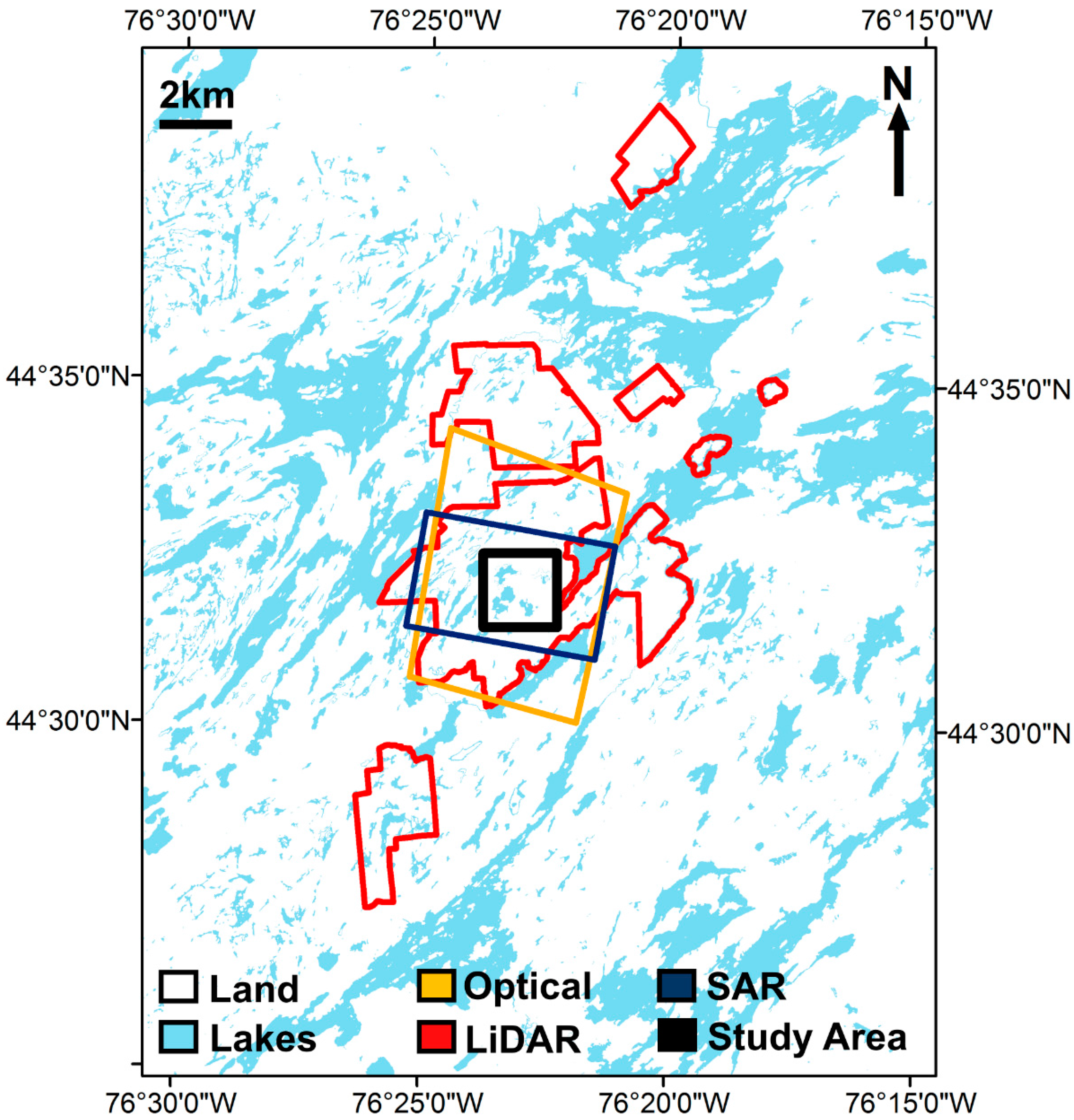
Figure 2.
Five in situ field work locations in study area: (A) Poole Lake; (B) Marsh A; (C) Inundated Forest; (D) Marsh B; and (E) Vegetated Lake.
Figure 2.
Five in situ field work locations in study area: (A) Poole Lake; (B) Marsh A; (C) Inundated Forest; (D) Marsh B; and (E) Vegetated Lake.

Figure 3.
Example of masks created using TSX data for 2 April 2016: (A) Processed SAR intensity image, greyscale with black representing low intensity values (−25 dB) and white representing high intensity values (0 dB); (B) SAR threshold water mask showing three classes—water (blue), uncertain (black), and non-water (white); (C) Error mask showing three classes; shadow commission zones in blue, layover omission zones in red, and no error in white; and (D) Final SAR water mask showing five classes representing the probability that a pixel is water.

Figure 4.
Decision tree analysis performed to create the final SAR water mask by combining the SAR threshold water mask with the shadow and layover zones with in text example highlighted in grey.
Figure 4.
Decision tree analysis performed to create the final SAR water mask by combining the SAR threshold water mask with the shadow and layover zones with in text example highlighted in grey.
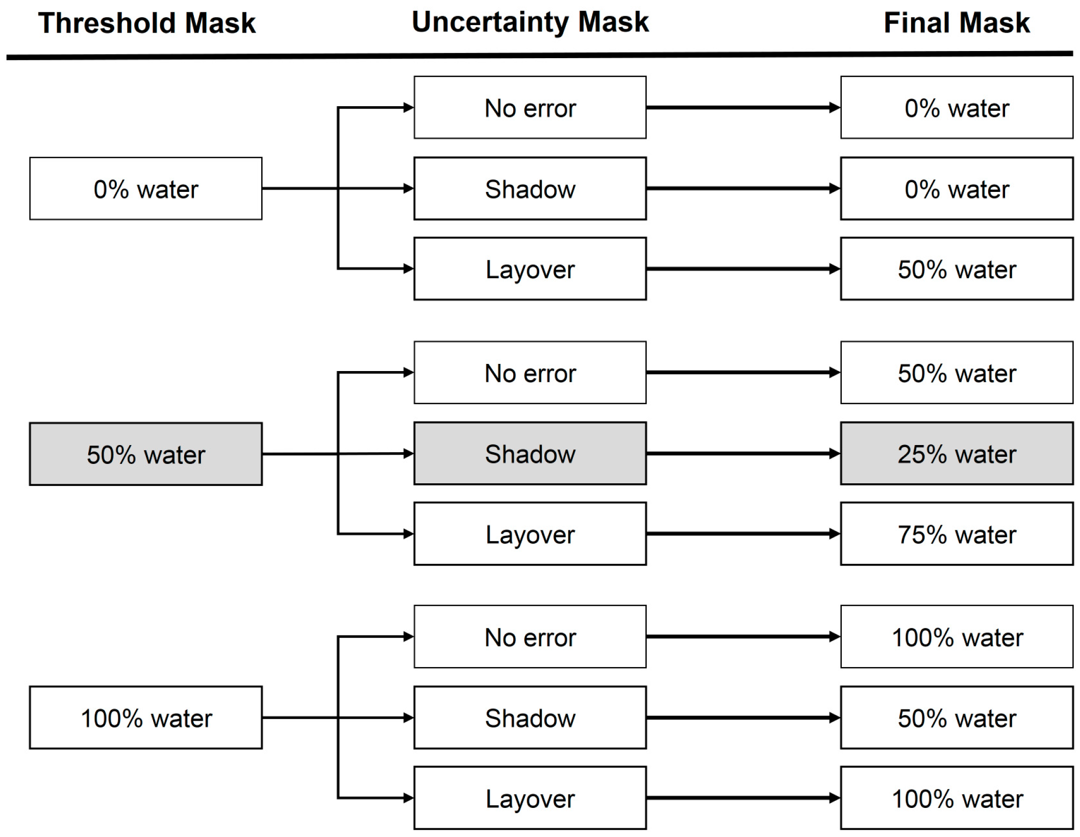
Figure 5.
Flow chart illustrating the tiered decision tree methodology used for classifying water using LiDAR data.
Figure 5.
Flow chart illustrating the tiered decision tree methodology used for classifying water using LiDAR data.

Figure 6.
Input parameters derived from LiDAR data to generate intermediate water masks: (A) Point density; (B) Intensity; (C) Scan angle; (D) Standard deviation of intensity; (E) Standard deviation of elevation; and (F) Pulse density of classified ground returns. Low values are in black, high values are in white.
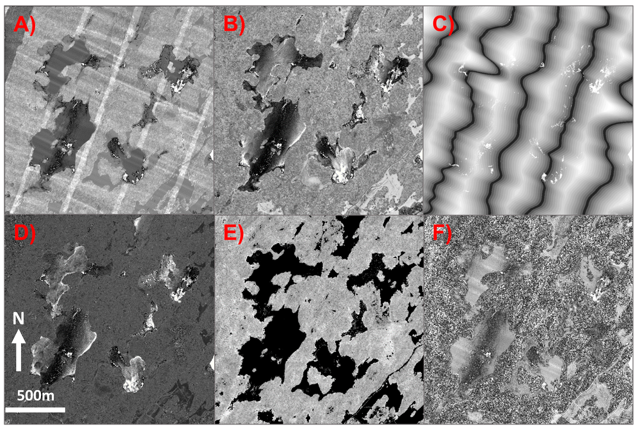
Figure 7.
Intermediate water masks derived from the input parameters using a decision tree, and the final water mask generated using LiDAR data: (A) Density water mask; (B) Intensity and Scan Angle water mask; (C) Standard Deviation water mask; (D) Inundation water mask; and (E) Final water mask classified using a decision tree with the intermediate water masks as input.

Figure 8.
Masks created using 8-band multispectral WorldView-2 imagery from 26 August 2016: (A) NDWI (Low values are in black, high values are in white); (B) Optical water mask showing two classes; water (blue), non-water (white); (C) NDVI (Low values are in black, high values are in white); (D) Error mask showing two classes; error/canopy zones in black, and no error in white; and (E) Final optical water mask showing three classes representing the probability that a pixel is water.

Figure 9.
Decision tree classifier used to create five fused water models from each of the SAR water masks combined with the LiDAR and optical water masks. The absolute differences at the pixel value of each water mask (PS, PL and PO) were calculated, and used to create eight different outcomes of which five occurred (white) and three did not occur (grey).

Figure 10.
Five fused water models created for the five SAR acquisition dates: 2 April, 24 April, 5 May, 10 July, and 3 September 2016. The three classes shown are non-water (white), uncertain (grey), water (blue). Rectangles outline the five study sub-areas.
Figure 10.
Five fused water models created for the five SAR acquisition dates: 2 April, 24 April, 5 May, 10 July, and 3 September 2016. The three classes shown are non-water (white), uncertain (grey), water (blue). Rectangles outline the five study sub-areas.

Figure 11.
Photographs from in situ fieldwork performed on three of the five SAR acquisition dates: in April, May and July 2016: (A) Poole Lake; (B) Marsh A; (C) Inundated Forest; (D) Marsh B; and (E) Vegetated Lake. This location was first observed on 5 May and also shows a photogrammetric model created using images captured from UAV.

Figure 12.
Five outcomes from the decision tree classifier and the LiDAR only additional statement showing the spatial extent of the sensor agreement from 2 April 2016. Black pixels represent areas where outcome occurred, white pixels represent areas where outcome did not occur: (A) All agree; (B) All disagree; (C) SAR disagree; (D) Optical disagree; (E) LiDAR disagree; and (F) LiDAR only.

Figure 13.
Five outcomes from the decision tree classifier and the LiDAR only additional statement showing the spatial extent of the sensor agreement from 3 September 2016. Black pixels represent areas where outcome occurred, white pixels represent areas where outcome did not occur: (A) All agree; (B) All disagree; (C) SAR disagree; (D) Optical disagree; (E) LiDAR disagree; and (F) LiDAR only.
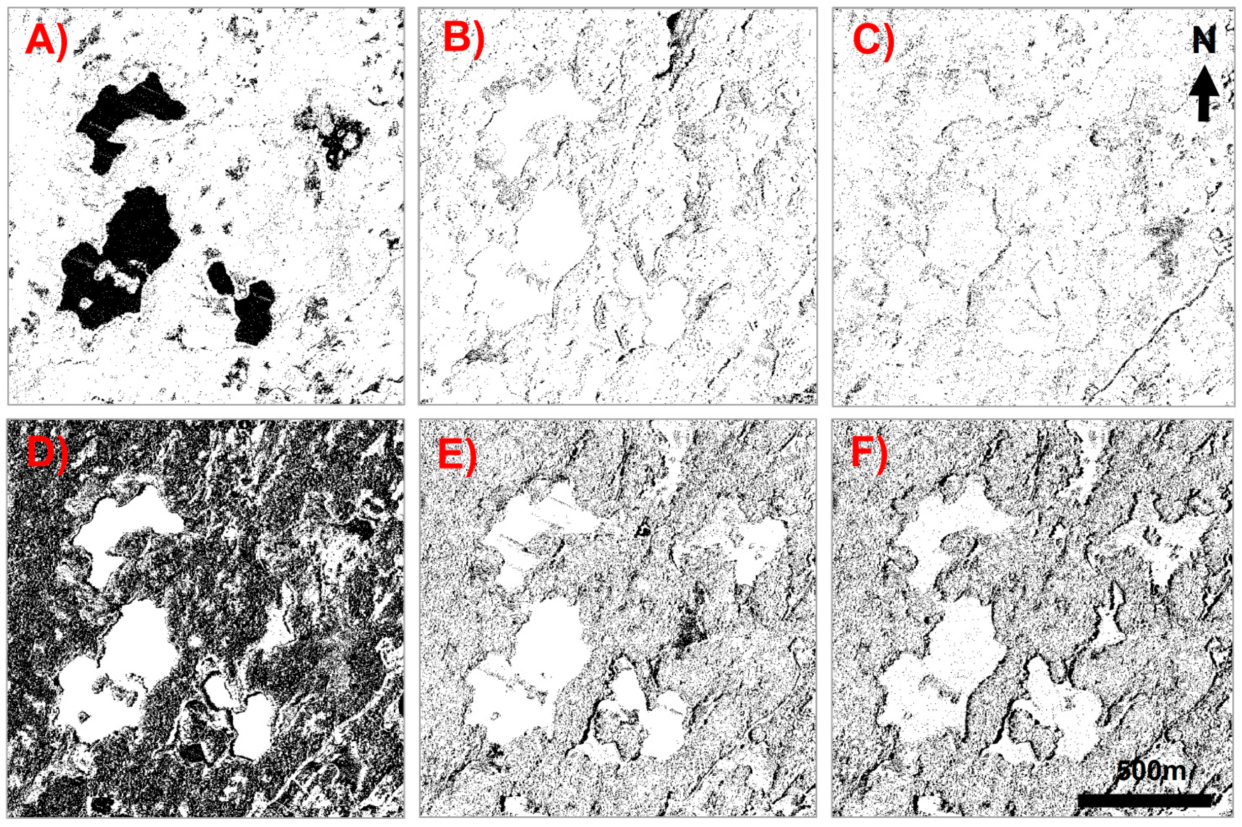
Figure 14.
Percent of pixels of the five outcomes from the sensor agreement models and the LiDAR only additional statement through time of SAR acquisition dates, also showing LiDAR acquisition month (June) and optical acquisition month (August).
Figure 14.
Percent of pixels of the five outcomes from the sensor agreement models and the LiDAR only additional statement through time of SAR acquisition dates, also showing LiDAR acquisition month (June) and optical acquisition month (August).

Table 1.
Summary of TSX, airborne LiDAR and satellite-based optical imagery data used in this study.
Table 1.
Summary of TSX, airborne LiDAR and satellite-based optical imagery data used in this study.
| Data Type | Date Acquired | Platform/Mission Details |
|---|---|---|
| Optical | 26 August 2016 | WorldView-2 multispectral imagery (8-band) |
| LiDAR | 10–11 June 2015 | Airborne LiDAR |
| SAR 1 | 2 April 2016 | TSX staring spotlight mode |
| SAR 2 | 24 April 2016 | TSX staring spotlight mode |
| SAR 3 | 5 May 2016 | TSX staring spotlight mode |
| SAR 4 | 10 July 2016 | TSX staring spotlight mode |
| SAR 5 | 3 September 2016 | TSX staring spotlight mode |
| Field Investigation 1 | 2 April 2016 | Photographs and GPS coordinates |
| Field Investigation 2 | 5 May 2016 | Photographs and GPS coordinates |
| Field Investigation 3 | 10 July 2016 | Photographs and GPS coordinates |
Table 2.
Percent of water, uncertainty and non-water of all models.
| Model | Percent (%) | ||||
|---|---|---|---|---|---|
| Name | 100% water | Uncertain (13 to 88%) | 0% water | Total (%) | |
| 1 | Single: SAR 2 April | 19 | 17 | 64 | 100 |
| 2 | Single: SAR 24 April | 18 | 17 | 65 | 100 |
| 3 | Single: SAR 5 May | 18 | 17 | 65 | 100 |
| 4 | Single: SAR 10 July | 19 | 22 | 58 | 100 |
| 5 | Single: SAR 3 September | 20 | 23 | 57 | 100 |
| 6 | Single: LiDAR | 20 | 4 | 76 | 100 |
| 7 | Single: Optical | 11 | 75 | 13 | 100 |
| 8 | Fused (2 April) | 18 | 6 | 76 | 100 |
| 9 | Fused (24 April) | 18 | 4 | 78 | 100 |
| 10 | Fused (5 May) | 18 | 6 | 76 | 100 |
| 11 | Fused (10 July) | 18 | 8 | 75 | 100 |
| 12 | Fused (3 September) | 17 | 9 | 74 | 100 |
© 2017 by the authors. Licensee MDPI, Basel, Switzerland. This article is an open access article distributed under the terms and conditions of the Creative Commons Attribution (CC BY) license (http://creativecommons.org/licenses/by/4.0/).
Share and Cite
MDPI and ACS Style
Irwin, K.; Beaulne, D.; Braun, A.; Fotopoulos, G. Fusion of SAR, Optical Imagery and Airborne LiDAR for Surface Water Detection. Remote Sens. 2017, 9, 890. https://doi.org/10.3390/rs9090890
AMA Style
Irwin K, Beaulne D, Braun A, Fotopoulos G. Fusion of SAR, Optical Imagery and Airborne LiDAR for Surface Water Detection. Remote Sensing. 2017; 9(9):890. https://doi.org/10.3390/rs9090890
Chicago/Turabian StyleIrwin, Katherine, Danielle Beaulne, Alexander Braun, and Georgia Fotopoulos. 2017. "Fusion of SAR, Optical Imagery and Airborne LiDAR for Surface Water Detection" Remote Sensing 9, no. 9: 890. https://doi.org/10.3390/rs9090890
Note that from the first issue of 2016, this journal uses article numbers instead of page numbers. See further details here.