Lidar Aboveground Vegetation Biomass Estimates in Shrublands: Prediction, Uncertainties and Application to Coarser Scales

 , ,
, ,  , and
, and
Abstract
:
1. Introduction
2. Study Area and Data
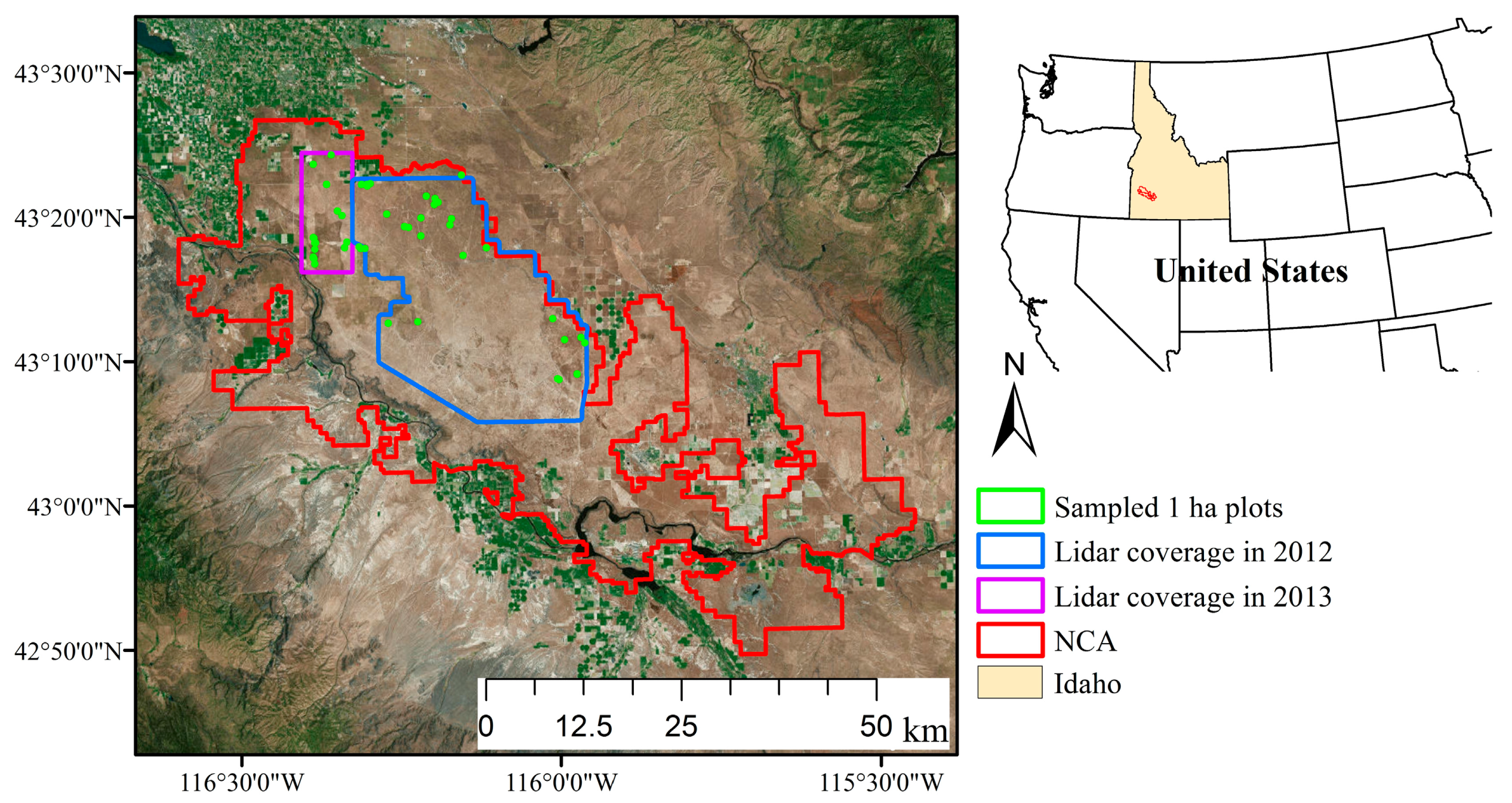
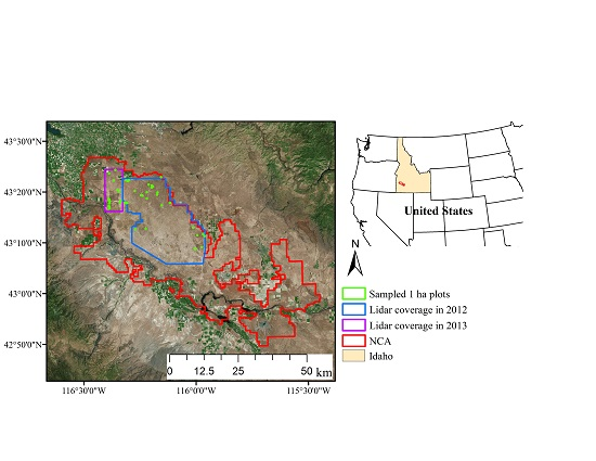
2.1. Study Area
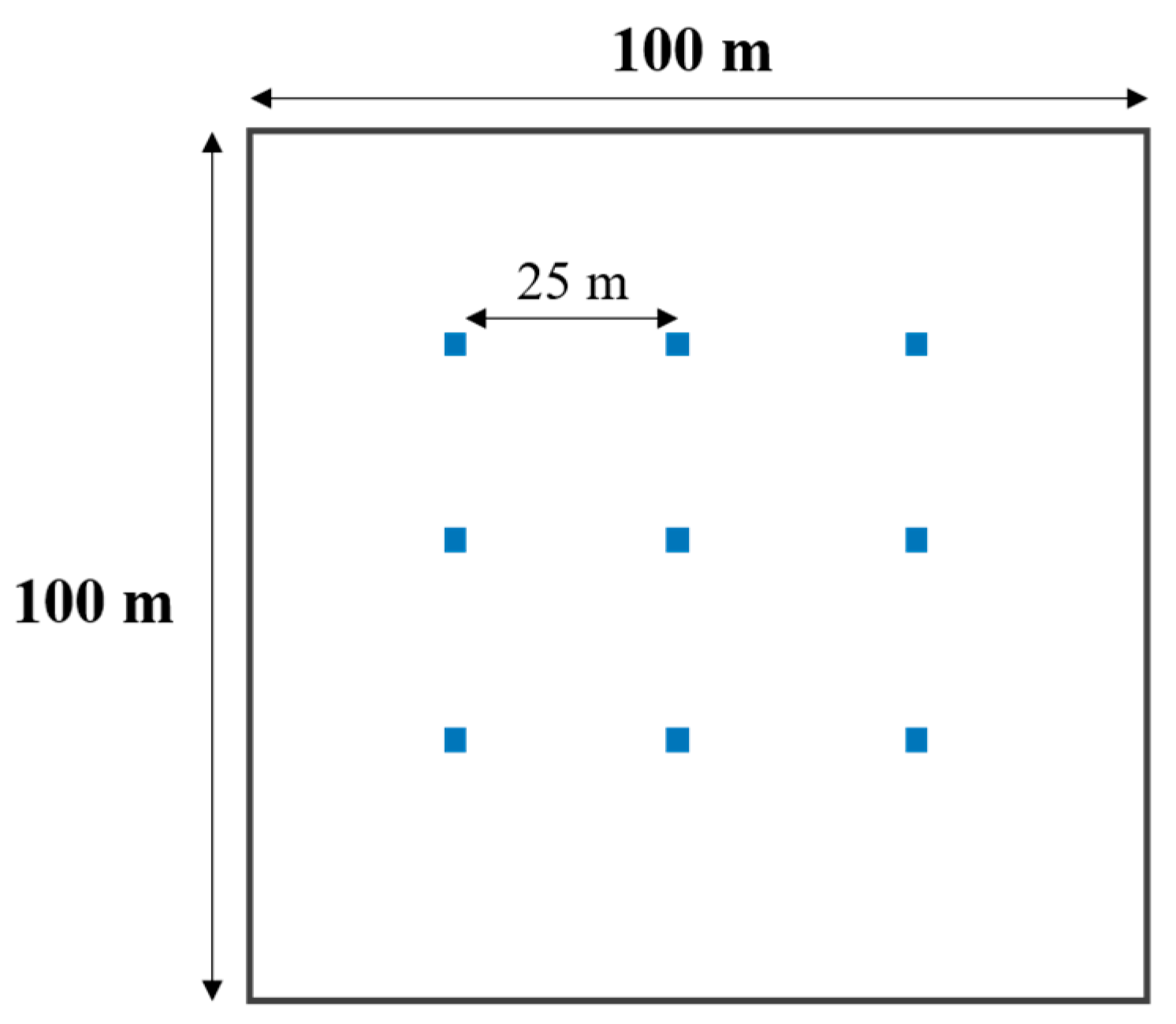
2.2. Field Sampling
2.3. Airborne Lidar Data Acquisitions
3. Methodology
3.1. Data Processing
3.2. Moldeing Plot-Scale Biomass
3.2.1. RF Regression Model
3.2.2. SMR Model
3.3. Imputation of Regional Biomass and Uncertainty
4. Results
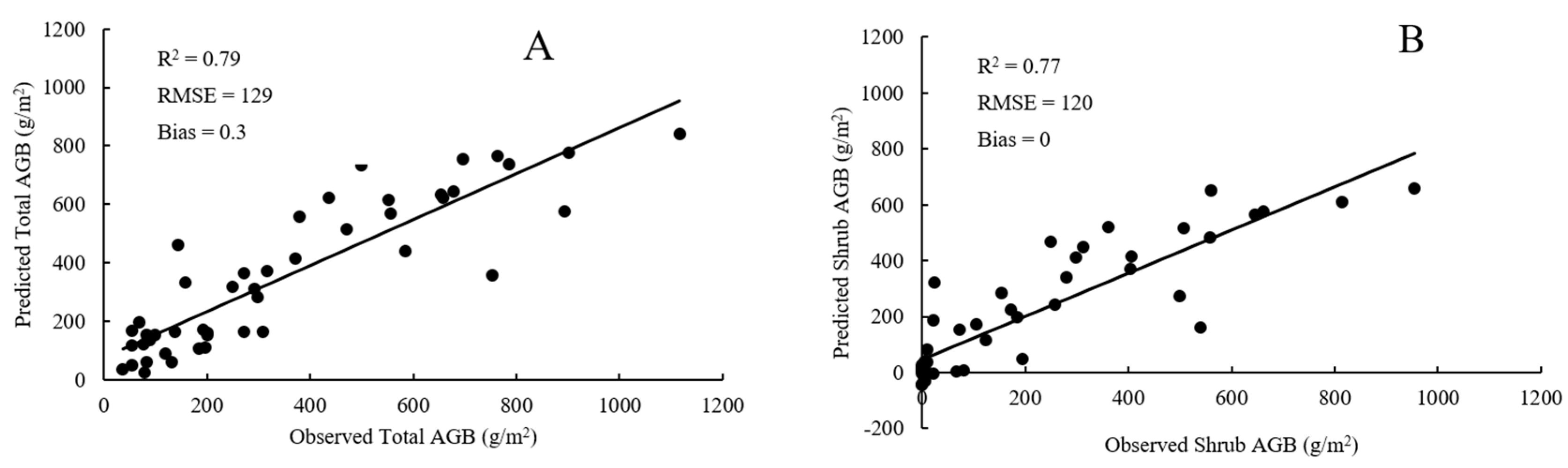
4.1. Plot-Scale Biomass from Raster-Derived Vegetation Metrics
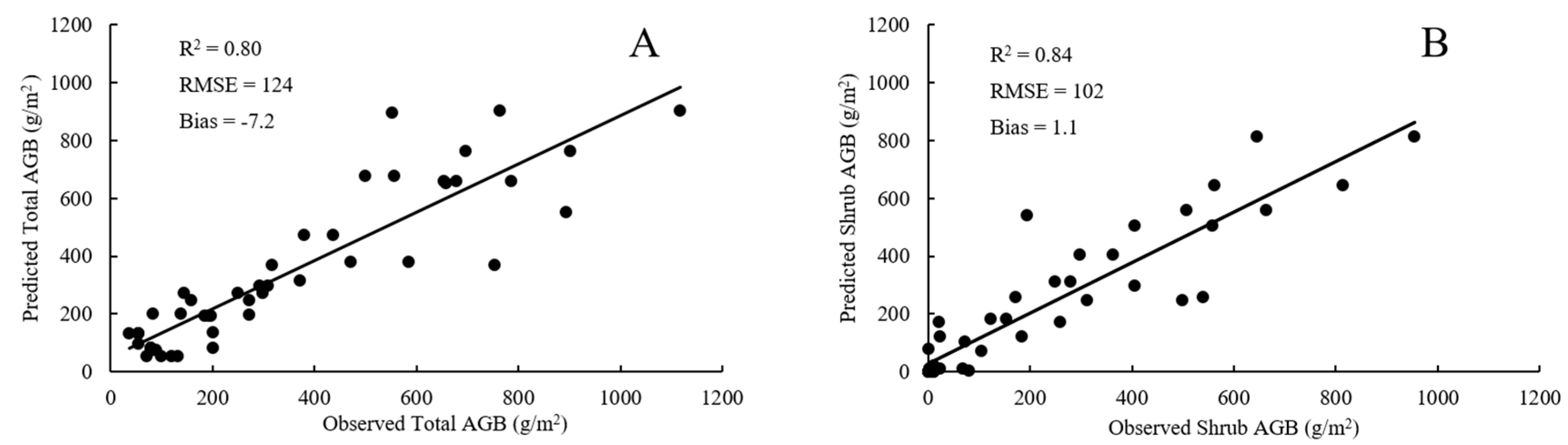
4.2. Plot-Scale Biomass from Point Cloud-Derived Vegetation Metrics
4.3. Comparison of RF Model and SMR Model
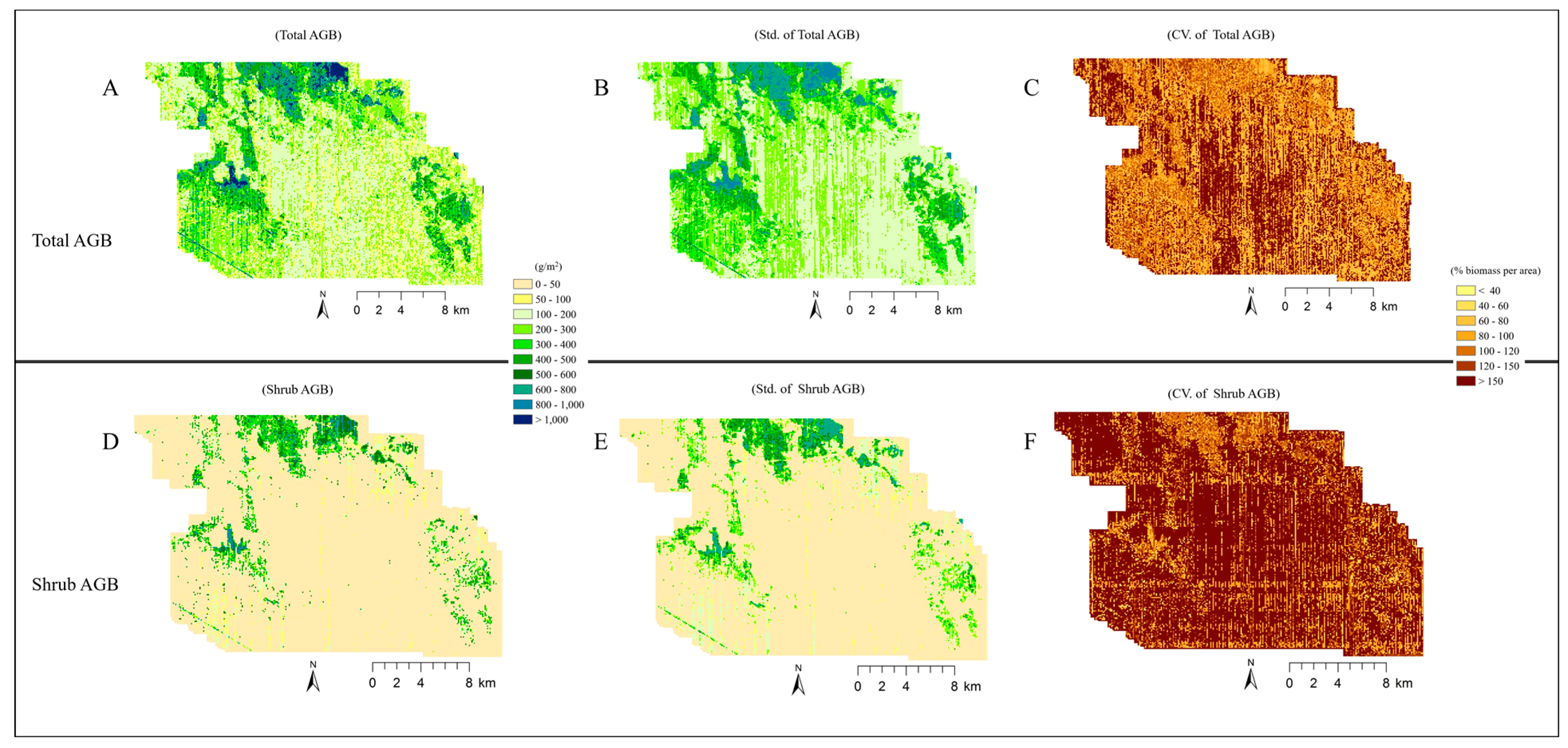
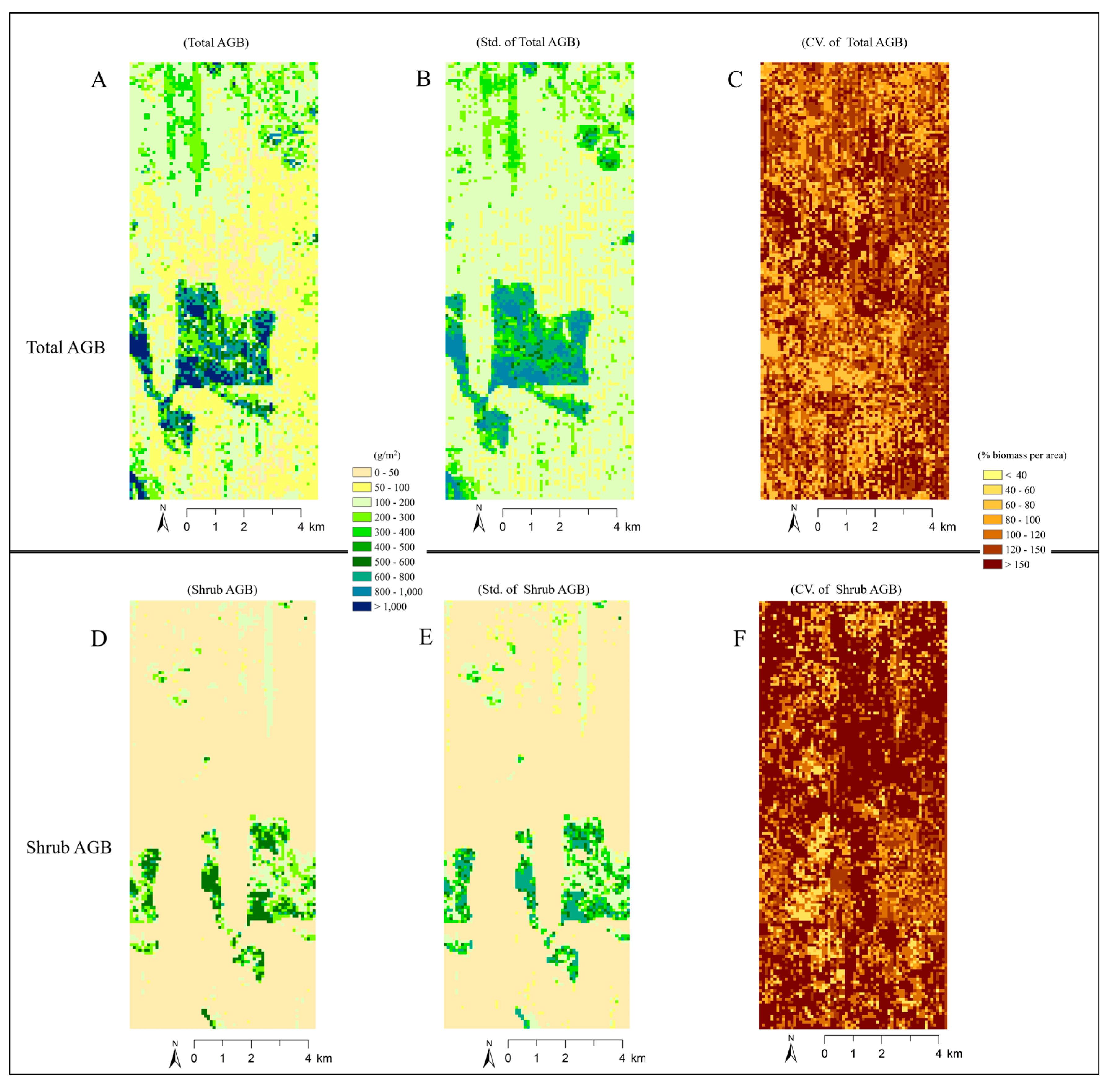
4.4. Analysis of Imputed Regional Biomass
5. Discussion
5.1. RF Biomass Regression Model
5.1.1. Uncertainty
5.1.2. RF Regression Model Variables
5.2. Model Performances of RF and SMR
5.3. Broader Application of the Imputed Shrub Biomass
6. Conclusions
Acknowledgments
Author Contributions
Conflicts of Interest
References
- Angell, R.F.; Svejcar, T.; Bates, J.; Saliendra, N.Z.; Johnson, D.A. Bowen ratio and closed chamber carbon dioxide flux measurements over sagebrush steppe vegetation. Agric. For. Meteorol. 2001, 108, 153–161. [Google Scholar] [CrossRef]
- Shrestha, G.; Stahl, P.D. Carbon accumulation and storage in semi-arid sagebrush steppe: Effects of long-term grazing exclusion. Agric. Ecosyst. Environ. 2008, 125, 173–181. [Google Scholar] [CrossRef]
- Rengsirikul, K.; Kanjanakuha, A.; Ishii, Y.; Kangvansaichol, K.; Sripichitt, P.; Punsuvon, V.; Vaithanomsat, P.; Nakamanee, G.; Tudsri, S. Potential forage and biomass production of newly introduced varieties of leucaena (Leucaena leucocephala (Lam.) de Wit.) in Thailand. Grassl. Sci. 2011, 57, 94–100. [Google Scholar] [CrossRef]
- Perez-Quezada, J.F.; Delpiano, C.A.; Snyder, K.A.; Johnson, D.A.; Franck, N. Carbon pools in an arid shrubland in Chile under natural and afforested conditions. J. Arid Environ. 2011, 75, 29–37. [Google Scholar] [CrossRef]
- Zandler, H.; Brenning, A.; Samimi, C. Quantifying dwarf shrub biomass in an arid environment: Comparing empirical methods in a high dimensional setting. Remote Sens. Environ. 2015, 158, 140–155. [Google Scholar] [CrossRef]
- Barbour, M.G.; Billings, W.D. North American Terrestrial Vegetation; Cambridge University Press: Cambridge, UK, 2000; ISBN 0-521-55027-0. [Google Scholar]
- Miller, R.F.; Knick, S.T.; Pyke, D.A.; Meinke, C.W.; Hanser, S.E.; Wisdom, M.J.; Hild, A.L. Characteristics of sagebrush habitats and limitations to long-term conservation. Greater sage-grouse: Ecology and conservation of a landscape species and its habitats. Stud. Avian Biol. 2011, 38, 145–184. [Google Scholar]
- Anderson, J.E.; Inouye, R.S. Landscape-scale changes in plant species abundance and biodiversity of a sagebrush steppe over 45 years. Ecol. Monogr. 2011, 71, 531–556. [Google Scholar] [CrossRef]
- Creutzburg, M.K.; Halofsky, J.E.; Halofsky, J.S.; Christopher, T.A. Climate change and land management in the rangelands of central Oregon. Environ. Manag. 2015, 55, 43–55. [Google Scholar] [CrossRef] [PubMed]
- Pyke, D.A.; Chambers, J.C.; Beck, J.L.; Brooks, M.L.; Mealor, B.A. Land uses, fire, and invasion: Exotic annual Bromus and human dimensions. In Exotic Brome-Grasses in Arid and Semiarid Ecosystems of the Western US: Causes, Consequences, and Management Implications; Germino, M.J., Chambers, J.C., Brown, C.S., Eds.; Springer International Publishing: Basel, Switzerland, 2016; pp. 307–336. ISBN 978-3-319-24928-5. [Google Scholar]
- Integrated Rangeland Fire Management Strategy Actionable Science Plan Team. The Integrated Rangeland Fire Management Strategy Actionable Science Plan; U.S. Department of the Interior: Washington, DC, USA, 2016; p. 128. Available online: https://www.fs.fed.us/rm/pubs_journals/2016/rmrs_2016_berg_k001.pdf (accessed on 29 August 2017).
- Sala, O.E.; Lauenroth, W.K. Small rainfall events: An ecological role in semiarid regions. Oecologia 1982, 53, 301–304. [Google Scholar] [CrossRef] [PubMed]
- Clark, P.E.; Hardegree, S.P.; Moffet, C.A.; Pierson, F.B. Point sampling to stratify biomass variability in sagebrush steppe vegetation. Rangel. Ecol. Manag. 2008, 61, 614–622. [Google Scholar] [CrossRef]
- Bonham, C.D. Measurements for Terrestrial Vegetation; John Wiley & Sons: Chichester, UK, 2013; ISBN 978-0-4709-7258-8. [Google Scholar]
- Waite, R.B. The application of visual estimation procedures for monitoring pasture yield and composition in exclosures and small plots. Trop. Grassl. 1994, 28, 38–42. [Google Scholar]
- Li, A.; Glenn, N.F.; Olsoy, P.J.; Mitchell, J.J.; Shrestha, R. Aboveground biomass estimates of sagebrush using terrestrial and airborne Lidar data in a dryland ecosystem. Agric. For. Meteorol. 2015, 213, 138–147. [Google Scholar] [CrossRef]
- Greaves, H.E.; Vierling, L.A.; Eitel, J.U.; Boelman, N.T.; Magney, T.S.; Prager, C.M.; Griffin, K.L. High-resolution mapping of aboveground shrub biomass in Arctic tundra using airborne Lidar and imagery. Remote Sens. Environ. 2016, 184, 361–373. [Google Scholar] [CrossRef]
- Powell, S.L.; Cohen, W.B.; Healey, S.P.; Kennedy, R.E.; Moisen, G.G.; Pierce, K.B.; Ohmann, J.L. Quantification of live aboveground forest biomass dynamics with Landsat time-series and field inventory data: A comparison of empirical modeling approaches. Remote Sens. Environ. 2010, 114, 1053–1068. [Google Scholar] [CrossRef]
- Lefsky, M.A.; Cohen, W.B.; Parker, G.G.; Harding, D.J. Lidar remote sensing for ecosystem studies. Bioscience 2002, 52, 19–30. [Google Scholar] [CrossRef]
- Hall, S.A.; Burke, I.C.; Box, D.O.; Kaufmann, M.R.; Stoker, J.M. Estimating stand structure using discrete-return Lidar: An example from low density, fire prone ponderosa pine forests. For. Ecol. Manag. 2005, 208, 189–209. [Google Scholar] [CrossRef]
- Ku, N.W.; Popescu, S.C.; Ansley, R.J.; Perotto-Baldivieso, H.L.; Filippi, A.M. Assessment of available rangeland woody plant biomass with a terrestrial LIDAR system. Photogramm. Eng. Remote Sens. 2012, 78, 349–361. [Google Scholar] [CrossRef]
- Lin, Y.; Hyyppä, J.; Kukko, A.; Jaakkola, A.; Kaartinen, H. Tree height growth measurement with single-scan airborne, static terrestrial and mobile laser scanning. Sensors 2012, 12, 12798–12813. [Google Scholar] [CrossRef] [PubMed]
- Zheng, G.; Moskal, L.M.; Kim, S.H. Retrieval of effective leaf area index in heterogeneous forests with terrestrial laser scanning. IEEE Trans. Geosci. Remote Sens. 2013, 51, 777–786. [Google Scholar] [CrossRef]
- Streutker, D.R.; Glenn, N.F. Lidar measurement of sagebrush steppe vegetation heights. Remote Sens. Environ. 2006, 102, 135–145. [Google Scholar] [CrossRef]
- Su, J.G.; Bork, E.W. Characterization of diverse plant communities in Aspen Parkland rangeland using Lidar data. Appl. Veg. Sci. 2007, 10, 407–416. [Google Scholar] [CrossRef]
- Glenn, N.F.; Spaete, L.P.; Sankey, T.T.; Derryberry, D.R.; Hardegree, S.P.; Mitchell, J.J. Errors in Lidar-derived shrub height and crown area on sloped terrain. J. Arid Environ. 2011, 75, 377–382. [Google Scholar] [CrossRef]
- Bork, E.W.; Su, J.G. Integrating LIDAR data and multispectral imagery for enhanced classification of rangeland vegetation: A meta analysis. Remote Sens. Environ. 2007, 111, 11–24. [Google Scholar] [CrossRef]
- García-Gutiérrez, J.; González-Ferreiro, E.; Mateos-García, D.; Riquelme-Santos, J.C.; Miranda, D. A comparative study between two regression methods on Lidar data: A case Study. In Hybrid Artificial Intelligent Systems HAIS 2011, Proceedings of the International Conference on Hybrid Artificial Intelligence Systems, Wrocław, Poland, 23–25 May 2011; Corchado, E., Kurzyński, M., Woźniak, M., Eds.; Lecture Notes in Computer Science; Springer: Berlin/Heidelberg, Germany, 2011; Volume 6679. [Google Scholar]
- Laurin, G.V.; Chen, Q.; Lindsell, J.A.; Coomes, D.A.; Del Frate, F.; Guerriero, L.; Pirotti, F.; Valentini, R. Above ground biomass estimation in an African tropical forest with Lidar and hyperspectral data. ISPRS J. Photogramm. Remote Sens. 2014, 89, 49–58. [Google Scholar] [CrossRef]
- Wilson, A.M.; Silander, J.A.; Gelfand, A.; Glenn, J.H. Scaling up: Linking field data and remote sensing with a hierarchical model. Int. J. Geogr. Inf. Sci. 2011, 25, 509–521. [Google Scholar] [CrossRef]
- Hudak, A.T.; Crookston, N.L.; Evans, J.S.; Hall, D.E.; Falkowski, M.J. Nearest neighbor imputation of species-level, plot-scale forest structure attributes from Lidar data. Remote Sens. Environ. 2008, 112, 2232–2245. [Google Scholar] [CrossRef]
- Debouk, H.; Riera-Tatché, R.; Vega-García, C. Assessing post-fire regeneration in a Mediterranean mixed forest using Lidar data and artificial neural networks. Photogramm. Eng. Remote Sens. 2013, 79, 1121–1130. [Google Scholar] [CrossRef]
- Breiman, L. Random Forests. Mach. Learn. 2001, 45, 5–32. [Google Scholar] [CrossRef]
- Breidenbach, J.; Næsset, E.; Lien, V.; Gobakken, T.; Solberg, S. Prediction of species specific forest inventory attributes using a nonparametric semi-individual tree crown approach based on fused airborne laser scanning and multispectral data. Remote Sens. Environ. 2010, 114, 911–924. [Google Scholar] [CrossRef]
- Vauhkonen, J.; Korpela, I.; Maltamo, M.; Tokola, T. Imputation of single-tree attributes using airborne laser scanning-based height, intensity, and alpha shape metrics. Remote Sens. Environ. 2010, 114, 1263–1276. [Google Scholar] [CrossRef]
- Guan, H.; Yu, J.; Li, J.; Luo, L. Random Forests-Based Feature Selection for Land-Use Classification Using LIDAR Data and Orthoimagery. International Archives of the Photogrammetry. Remote Sens. Spat. Inf. Sci. 2012, 39, B7. [Google Scholar]
- Mitchell, J.J.; Shrestha, R.; Moore-Ellison, C.A.; Glenn, N.F. Single and multi-date Landsat classifications of basalt to support soil survey efforts. Remote Sens. 2013, 5, 4857–4876. [Google Scholar] [CrossRef]
- Gleason, C.J.; Im, J. Forest biomass estimation from airborne Lidar data using machine learning approaches. Remote Sens. Environ. 2012, 125, 80–91. [Google Scholar] [CrossRef]
- Prasad, A.M.; Iverson, L.R.; Liaw, A. Newer classification and regression tree techniques: Bagging and random forests for ecological prediction. Ecosystems 2006, 9, 181–199. [Google Scholar] [CrossRef]
- Mutanga, O.; Adam, E.; Cho, M.A. High density biomass estimation for wetland vegetation using WorldView-2 imagery and random forest regression algorithm. Int. J. Appl. Earth Obs. Geoinf. 2012, 18, 399–406. [Google Scholar] [CrossRef]
- Mitchell, J.J.; Shrestha, R.; Spaete, L.P.; Glenn, N.F. Combining airborne hyperspectral and Lidar data across local sites for upscaling shrubland structural information: Lessons for HyspIRI. Remote Sens. Environ. 2015, 167, 98–110. [Google Scholar] [CrossRef]
- Passalacqua, P.; Belmont, P.; Staley, D.M.; Simley, J.D.; Arrowsmith, J.R.; Bode, C.A.; Crosby, C.; DeLong, S.B.; Glenn, N.F.; Kelly, S.A.; et al. Analyzing high resolution topography for advancing the understanding of mass and energy transfer through landscapes: A review. Earth Sci. Rev. 2015, 148, 174–193. [Google Scholar] [CrossRef] [Green Version]
- El-Ashmawy, N.; Shaker, A. Raster vs. Point Cloud Lidar Data Classification. Int. Arch. Photogramm. Remote Sens. Spat. Inf. Sci. 2014, 40, 79. [Google Scholar] [CrossRef]
- Western Region Climate Center (WRCC). Swan Falls Power House, Idaho, Period of Record General Climate Summary. 2012. Available online: http://www.wrcc.dri.edu/cgi-bin/cliMAIN.pl?id8928 (accessed on 1 June 2017).
- Anderson, K. Vegetation Measurement in Sagebrush Steppe Using Terrestrial Laser Scanning. Master’s Thesis, Idaho State University, Pocatello, ID, USA, 2014. [Google Scholar]
- U.S. Department of the Interior; Bureau of Land Management; Boise District Office. Snake River Birds of Prey National Conservation Area Proposed Resource Management Plan and Final Environmental Impact Statement. 2008. Available online: https://eplanning.blm.gov/epl-front-office/projects/lup/35553/41909/44409/SRBOPA_NCA_FEIS_V2_Appendices_508.pdf (accessed on 1 June 2017).
- Shinneman, D.J.; Arkle, R.; Pilliod, D.; Glenn, N.F. Quantifying and Predicting Fuels and the Effects of Reduction Treatments along Successional and Invasion Gradients in Sagebrush Habitats. Final Report to the Joint Fire Science Program; 2015; pp. 1–44. Available online: https://www.firescience.gov/projects/11-1-2-30/project/11-1-2-30_final_report.pdf (accessed on 1 June 2017).
- Pilliod, D.S.; Arkle, R.S. Performance of quantitative sampling methods across gradients of cover in Great Basin plant communities. Rangel. Ecol. Manag. 2013, 66, 634–647. [Google Scholar] [CrossRef]
- Spaete, L.P.; Glenn, N.F.; Baun, C.W. 2013 Morley Nelson Snake River Birds of Prey National Conservation Area RapidEye 7 m Landcover Classification; Boise State University: Boise, ID, USA, 2016; Available online: http://dx.doi.org/10.18122/B21592 (accessed on 1 June 2017).
- Glenn, N.F.; Neuenschwander, A.; Vierling, L.A.; Spaete, L.; Li, A.; Shinneman, D.J.; McIlroy, S.K. Landsat 8 and ICESat-2: Performance and potential synergies for quantifying dryland ecosystem vegetation cover and biomass. Remote Sens. Environ. 2016, 185, 233–242. [Google Scholar] [CrossRef]
- Painter, T.H.; Berisford, D.F.; Boardman, J.W.; Bormann, K.J.; Deems, J.S.; Gehrke, F.; Hedrick, A.; Joyce, M.; Laidlaw, R.; Marks, D.; et al. The Airborne Snow Observatory: Fusion of scanning Lidar, imaging spectrometer, and physically-based modeling for mapping snow water equivalent and snow albedo. Remote Sens. Environ. 2016, 184, 139–152. [Google Scholar] [CrossRef]
- Naidoo, L.; Cho, M.A.; Mathieu, R.; Asner, G. Classification of savanna tree species, in the Greater Kruger National Park region, by integrating hyperspectral and Lidar data in a Random Forest data mining environment. ISPRS J. Photogramm. Remote Sens. 2012, 69, 167–179. [Google Scholar] [CrossRef]
- Prinzie, A.; Van den Poel, D. Random forests for multiclass classification: Random multinomial logit. Expert Syst. Appl. 2008, 34, 1721–1732. [Google Scholar] [CrossRef]
- Ismail, R.; Mutanga, O.; Kumar, L. Modeling the potential distribution of pine forests susceptible to sirex noctilio infestations in Mpumalanga, South Africa. Trans. GIS 2010, 14, 709–726. [Google Scholar] [CrossRef]
- Montgomery, D.C.; Peck, E.A.; Vining, G.G. Introduction to Linear Regression Analysis; John Wiley & Sons: Hoboken, NJ, USA, 2015; ISBN 978-0-470-54281-1. [Google Scholar]
- Lefsky, M.A.; Cohen, W.B.; Harding, D.J.; Parker, G.G.; Acker, S.A.; Gower, S.T. Lidar remote sensing of above-ground biomass in three biomes. Glob. Ecol. Biogeogr. 2002, 11, 393–399. [Google Scholar] [CrossRef]
- Hudak, A.; Evans, J.S.; Crookstone, N.L.; Falkowski, M.J.; Steigers, B.K.; Taylor, R.; Hemingway, H. Aggregating pixel-level basal area predictions derived from Lidar data to industrial forest stands in North-Central Idaho. In Proceedings of the Third Forest Vegetation Simulator Conference, Fort Collins, CO, USA, 13–15 February 2007; pp. 133–145. [Google Scholar]
- Eskelson, B.N.; Temesgen, H.; Lemay, V.; Barrett, T.M.; Crookston, N.L.; Hudak, A.T. The roles of nearest neighbor methods in imputing missing data in forest inventory and monitoring databases. Scand. J. For. Res. 2009, 24, 235–246. [Google Scholar] [CrossRef]
- Crookston, N.L.; Finley, A.O. yaImpute: An R Package for kNN Imputation. J. Stat. Softw. 2008, 23, 1–16. [Google Scholar] [CrossRef]
- Strobl, C.; Malley, J.; Tutz, G. An introduction to recursive partitioning: Rationale, application, and characteristics of classification and regression trees, bagging, and random forests. Psychol. Methods 2009, 14, 323–348. [Google Scholar] [CrossRef] [PubMed] [Green Version]
- Olsoy, P.J.; Glenn, N.F.; Clark, P.E.; Derryberry, D.R. Aboveground total and green biomass of dryland shrub derived from terrestrial laser scanning. ISPRS J. Photogramm. Remote Sens. 2014, 88, 166–173. [Google Scholar] [CrossRef]
- Olsoy, P.J.; Glenn, N.F.; Clark, P.E. Estimating sagebrush biomass using terrestrial laser scanning. Rangel. Ecol. Manag. 2014, 67, 224–228. [Google Scholar] [CrossRef]
- Greaves, H.E.; Vierling, L.A.; Eitel, J.U.; Boelman, N.T.; Magney, T.S.; Prager, C.M.; Griffin, K.L. Estimating aboveground biomass and leaf area of low-stature Arctic shrubs with terrestrial Lidar. Remote Sens. Environ. 2015, 164, 26–35. [Google Scholar] [CrossRef]
- Ni-Meister, W.; Lee, S.; Strahler, A.H.; Woodcock, C.E.; Schaaf, C.; Yao, T.; Ranson, K.J.; Sun, G.; Blair, J.B. Assessing general relationships between aboveground biomass and vegetation structure parameters for improved carbon estimate from Lidar remote sensing. J. Geophys. Res. Biogeosci. 2010, 115. [Google Scholar] [CrossRef]
- Spaete, L.P.; Glenn, N.F.; Derryberry, D.R.; Sankey, T.T.; Mitchell, J.J.; Hardegree, S.P. Vegetation and slope effects on accuracy of a Lidar-derived DEM in the sagebrush steppe. Remote Sens. Lett. 2011, 2, 317–326. [Google Scholar] [CrossRef]
- Mitchell, J.J.; Glenn, N.F.; Sankey, T.T.; Derryberry, D.R.; Anderson, M.O.; Hruska, R.C. Small-footprint Lidar estimations of sagebrush canopy characteristics. Photogramm. Eng. Remote Sens. 2011, 77, 521–530. [Google Scholar] [CrossRef]
- Riaño, D.; Chuvieco, E.; Ustin, S.L.; Salas, J.; Rodríguez-Pérez, J.R.; Ribeiro, L.M.; Viegas, D.X.; Moreno, J.M.; Fernández, H. Estimation of shrub height for fuel-type mapping combining airborne Lidar and simultaneous color infrared ortho imaging. Int. J. Wildland Fire 2007, 16, 341–348. [Google Scholar] [CrossRef]
- Estornell, J.; Ruiz, L.A.; Velázquez-Martí, B.; Hermosilla, T. Estimation of biomass and volume of shrub vegetation using Lidar and spectral data in a Mediterranean environment. Biomass Bioenergy 2012, 46, 710–721. [Google Scholar] [CrossRef]
- Mundt, J.T.; Streutker, D.R.; Glenn, N.F. Mapping sagebrush distribution using fusion of hyperspectral and Lidar classifications. Photogramm. Eng. Remote Sens. 2006, 72, 47–54. [Google Scholar] [CrossRef]
- Whittingham, M.J.; Stephens, P.A.; Bradbury, R.B.; Freckleton, R.P. Why do we still use stepwise modelling in ecology and behaviour? J. Anim. Ecol. 2006, 75, 1182–1189. [Google Scholar] [CrossRef] [PubMed]
- Cutler, D.R.; Edwards, T.C.; Beard, K.H.; Cutler, A.; Hess, K.T.; Gibson, J.; Lawler, J.J. Random forests for classification in ecology. Ecology 2007, 88, 2783–2792. [Google Scholar] [CrossRef] [PubMed]
- Uresk, D.W.; Gilbert, R.O.; Rickard, W.H. Sampling big sagebrush for phytomass. J. Range Manag. 1977, 30, 311–314. [Google Scholar] [CrossRef]
- Brown, J.K. Fuel and Fire Behavior Prediction in Big Sagebrush. USDA Forest Service Research Paper INT (USA). 1982. Available online: https://www.fs.fed.us/rm/pubs_int/int_rp290.pdf (accessed on 1 June 2017).
- Cleary, M.B.; Pendall, E.; Ewers, B.E. Testing sagebrush allometric relationships across three fire chronosequences in Wyoming, USA. J. Arid Environ. 2008, 72, 285–301. [Google Scholar] [CrossRef]
- Sankey, T.; Shrestha, R.; Sankey, J.B.; Hardegree, S.P.; Strand, E. Lidar-derived estimate and uncertainty of carbon sink in successional phases of woody encroachment. J. Geophys. Res. Biogeosci. 2013, 118, 1144–1155. [Google Scholar] [CrossRef]
- Margolis, H.A.; Nelson, R.F.; Montesano, P.M.; Beaudoin, A.; Sun, G.; Andersen, H.E.; Wulder, M.A. Combining satellite Lidar, airborne Lidar, and ground plots to estimate the amount and distribution of aboveground biomass in the boreal forest of North America. Can. J. For. Res. 2015, 45, 838–855. [Google Scholar] [CrossRef]


| Herbaceous Cover (%) | Shrub Cover (%) | Herbaceous AGB (g/m2) | Shrub AGB (g/m2) | Total AGB (g/m2) | |
|---|---|---|---|---|---|
| Minimum | 23.4 | 0 | 31.1 | 0 | 36.8 |
| Maximum | 98.6 | 46.9 | 489.4 | 954.4 | 1116.8 |
| Mean ± Std. | 65 ± 20 | 12 ± 13 | 144 ± 87 | 208 ± 253 | 352 ± 281 |
| Lidar Metric | Description |
|---|---|
| Hmin | The minimum of all height points within each pixel |
| Hmax | The maximum of all height points within each pixel |
| Hrange | The difference of maximum and minimum of all height points within each pixel |
| Hmean | The average of all height points within each pixel |
| HMAD | The Median Absolute Deviation from Median Height value (HMAD) of all height points within each pixel, where HMAD = 1.4826 × median (|height − median height|) |
| HAAD | The Mean Absolute Deviation from Mean Height (HAAD) value of all height points within each pixel, where HAAD = mean (|height − mean height|) |
| Hvar | The variance of all height points within each pixel |
| Hstd | The standard deviation of all height points within each pixel |
| Hskew | The skewness of all height points within each pixel |
| Hkurt | The kurtosis of all height points within each pixel |
| HIQR | The Interquartile Range (HIQR) of all height points within each pixel, where HIQR = Q75 − Q25, where Qx is xth percentile |
| HCV | The coefficient of variation of all height points within each pixel |
| H5, H10 etc. | The 5th, 10th, 25th, 50th, 75th, 90th, and 95th percentiles of all height points within each pixel |
| nAll | The total number of all points within each pixel |
| nV | The total number of all the points within each pixel that are above the specified Crown Threshold value (CT) |
| nG | The total number of all the points within each pixel that are below the specified Ground Threshold value (GT) |
| Veg_density | The percent ratio of vegetation returns and ground returns within each pixel |
| Veg_cov | The percent ratio of vegetation returns and total returns within each pixel |
| pG | Percent of points within each pixel that are below the specified Ground Threshold |
| pH1, pH2.5 etc. | Percent of vegetation in height ranges 0–1 m, 1–2.5 m, 2.5–10 m, 10–20 m, 20–30 m, and >30 m within each pixel |
| CRR | Canopy relief ratio of points within each pixel, where CRR = ((Hmean − Hmin))/((Hmax − Hmin)) |
| Htext | Texture of height of points within each pixel, where Htext = St. Dev. (Height > GT and Height < CT) |
| FHDall | Foliage arrangement in the vertical direction (Foliage Height Diversity), where FHDall = −∑pi *lnpi where pi is the proportion of horizontal foliage coverage in the i-th layer to the sum of the foliage coverage of all the layers |
| FHDGT | FHD calculated only from the points above GT |
| Scale (m) | Pseudo R2 | RMSE (g/m2) | Predictors | |
|---|---|---|---|---|
| Total AGB | 1 | 0.74 | 141 | Hstd, HAAD, H90, HSkew, Hvar, Htext |
| 7 | 0.70 | 152 | Htext, FHDGT, H95, HAAD | |
| 30 | 0.58 | 180 | FHDGT, nV, HAAD, H5 | |
| 100 | 0.52 | 188 | FHDGT, nV, H16, HAAD | |
| Shrub AGB | 1 | 0.76 | 125 | Hstd, HAAD, HCV, Hrange, FHDall |
| 7 | 0.67 | 143 | Htext, FHDGT, HAAD | |
| 30 | 0.50 | 176 | FHDGT, HAAD, HCV | |
| 100 | 0.40 | 184 | Htext, H50, pG, nG |
| Scale (m) | Pseudo R2 | RMSE (g/m2) | Predictors | |
|---|---|---|---|---|
| Total AGB | 1 | 0.71 | 147 | HMAD, HSkew, HIQR, HAAD, Hstd, Hkurt, H90, HCV |
| 7 | 0.71 | 148 | Htext, HIQR | |
| 30 | 0.70 | 151 | HAAD, H95, HIQR, pH1, pG | |
| 100 | 0.67 | 160 | H90, H95, Htext, Veg_density | |
| Shrub AGB | 1 | 0.73 | 129 | HIQR, Hstd, HMAD, HCV |
| 7 | 0.72 | 132 | Htext, H90, HIQR, HCV | |
| 30 | 0.65 | 146 | H90, HIQR, Htext, pH1 | |
| 100 | 0.64 | 151 | H95, Htext, pH1, GIQR, FHDGT |
| Scale (m) | Source | Pseudo R2 | RMSE (g/m2) | Predictors | |
|---|---|---|---|---|---|
| Herbaceous AGB | 1 | Raster | 0.20 | 6.86 | HSkew, Htext |
| 1 | Point Cloud | 0.19 | 7.54 | HCV, Htext, HSkew |
| 2012 Lidar | 2013 Lidar | ||||
|---|---|---|---|---|---|
| Total AGB | Shrub AGB | Total AGB | Shrub AGB | ||
| Biomass (g/m2) | Minimum | 36.8 | 0 | 36.8 | 0 |
| Maximum | 1116.8 | 954.4 | 1116.8 | 662.5 | |
| Mean ± Std. | 263 ± 204 | 60 ± 149 | 210 ± 238 | 51 ± 126 | |
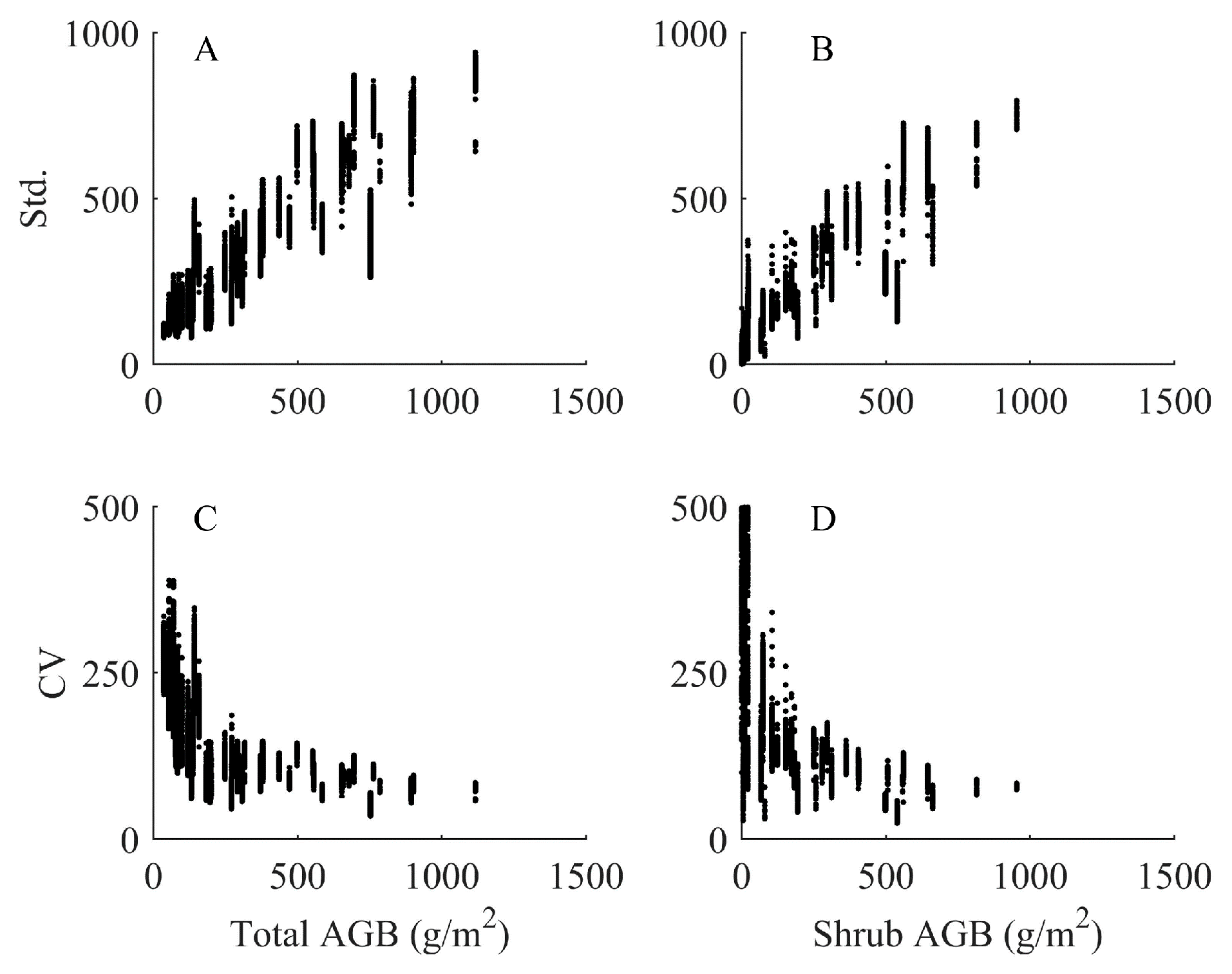
| CV (% biomass per area) | Minimum | 34.9 | 23.9 | 46.0 | 31.4 |
| Maximum | 389.2 | 499.9 | 347.9 | 495.0 | |
| Mean ± Std. | 121 ± 48 | 148 ± 102 | 136 ± 58 | 190 ± 90 | |
© 2017 by the authors. Licensee MDPI, Basel, Switzerland. This article is an open access article distributed under the terms and conditions of the Creative Commons Attribution (CC BY) license (http://creativecommons.org/licenses/by/4.0/).
Share and Cite
Li, A.; Dhakal, S.; Glenn, N.F.; Spaete, L.P.; Shinneman, D.J.; Pilliod, D.S.; Arkle, R.S.; McIlroy, S.K. Lidar Aboveground Vegetation Biomass Estimates in Shrublands: Prediction, Uncertainties and Application to Coarser Scales. Remote Sens. 2017, 9, 903. https://doi.org/10.3390/rs9090903
Li A, Dhakal S, Glenn NF, Spaete LP, Shinneman DJ, Pilliod DS, Arkle RS, McIlroy SK. Lidar Aboveground Vegetation Biomass Estimates in Shrublands: Prediction, Uncertainties and Application to Coarser Scales. Remote Sensing. 2017; 9(9):903. https://doi.org/10.3390/rs9090903
Chicago/Turabian StyleLi, Aihua, Shital Dhakal, Nancy F. Glenn, Lucas P. Spaete, Douglas J. Shinneman, David S. Pilliod, Robert S. Arkle, and Susan K. McIlroy. 2017. "Lidar Aboveground Vegetation Biomass Estimates in Shrublands: Prediction, Uncertainties and Application to Coarser Scales" Remote Sensing 9, no. 9: 903. https://doi.org/10.3390/rs9090903