Transfer Learning with Deep Convolutional Neural Network for SAR Target Classification with Limited Labeled Data


1
School of Electronic, Electrical and Communication Engineering, University of Chinese Academy of Sciences, Huairou District, Beijing 101408, China
2
Institute of Electronics, Chinese Academy of Sciences, Beijing 100190, China
3
Key Laboratory of Technology in Geo-spatial Information Processing and Application System, Beijing 100190, China
*
Author to whom correspondence should be addressed.
Remote Sens. 2017, 9(9), 907; https://doi.org/10.3390/rs9090907
Submission received: 7 July 2017
/
Revised: 20 August 2017
/
Accepted: 28 August 2017
/
Published: 31 August 2017
(This article belongs to the Special Issue Deep Learning for Target Object Detection and Identification in Remote Sensing Data)
Abstract
:Tremendous progress has been made in object recognition with deep convolutional neural networks (CNNs), thanks to the availability of large-scale annotated dataset. With the ability of learning highly hierarchical image feature extractors, deep CNNs are also expected to solve the Synthetic Aperture Radar (SAR) target classification problems. However, the limited labeled SAR target data becomes a handicap to train a deep CNN. To solve this problem, we propose a transfer learning based method, making knowledge learned from sufficient unlabeled SAR scene images transferrable to labeled SAR target data. We design an assembled CNN architecture consisting of a classification pathway and a reconstruction pathway, together with a feedback bypass additionally. Instead of training a deep network with limited dataset from scratch, a large number of unlabeled SAR scene images are used to train the reconstruction pathway with stacked convolutional auto-encoders (SCAE) at first. Then, these pre-trained convolutional layers are reused to transfer knowledge to SAR target classification tasks, with feedback bypass introducing the reconstruction loss simultaneously. The experimental results demonstrate that transfer learning leads to a better performance in the case of scarce labeled training data and the additional feedback bypass with reconstruction loss helps to boost the capability of classification pathway.
1. Introduction
Synthetic Aperture Radar automatic target recognition (SAR-ATR) has been a driving motivation for many years. Generally, the SAR-ATR system can be split into three stages: detection, low-level classification (LLC) and high-level classification (HLC). The first two stages that are also known as prescreening and discrimination together generate the focus-of-attention (FOA) module [1]. It interfaces with the input SAR images and outputs a list of potential SAR targets as the input of the HLC stage. Finally, the HLC stage aims to classify the targets into different categories, which is the main focus of this paper.
Various methods have been proposed to implement the HLC stage, which can be concluded as three taxonomies: feature-based, model-based and semi-model-based according to [1]. Feature-based approaches, extracting and preprocessing features from SAR target chips and training a classifier with them, are extensively used in the literature for HLC stage. To obtain a satisfactory classification performance, both the features and the classifiers should be carefully elaborately designed. On the one hand, various types of classifiers, such as sparse representation-based method [2], Bayes classifier [3], mean square error (MSE) classifier [4], template-based classifiers [5] and support vector machine (SVM) [6], are selected to solve the problem. Among them, the sparse representation classification is popular in recent studies [7,8]. The improved joint sparse representation model was proposed to effectively combine multiple-view SAR images from the same physical target [9]. Pan et al. [10] designed a reweighted sparse representation based method to suppress the influence of the interference caused by objects near the targets. In addition, better performance is proved on the fusion of multiple classifiers than the single classifier [11]. Liu et al. [12] proposed a decision fusion method of sparse representation and SVM, fusing the results of two classifiers obeying Bayesian rule to make the decision. On the other hand, hand-crafted features, for example, geometrical feature [13], principal components analysis (PCA) based features [3] and Fourier descriptors [6], as well as target chip templates [4,14], are extracted to feed into the classifiers conventionally. Due to the development of high-resolution SAR in recent years, new progress has been made to depict SAR images with more details. Carried in the magnitude of the radar backscatter, the scattering centers are considered as distinctive characteristics of SAR target images [15]. As depicted in [10], instead of using the scatter point extraction to describe the backscattering characteristic, a scatter cluster extraction method is proposed. Dense scale-invariant feature transform (SIFT) descriptors on multiple scales are used to train a global multi-scale dictionary by sparse coding algorithm [16]. Based on the probabilistic graphical models, Srinivas et al. [17] yields multiple SAR image representations and models each of them using graphs. The monogenic signal is performed to characterize the SAR images [18]. Most of the studies have carried out the experiments on Moving and Stationary Target Acquisition and Recognition (MSTAR) public dataset to evaluate their methods. The best result among the hand-crafted methods can achieve 97.33% on the MSTAR dataset for the 10-class recognition task [12].
Different from the hand-crafted feature extraction based method, the deep CNN based method automatically learns the feature from large-scale dataset, and achieves very impressive performance in object recognition. In computer vision domain, deep CNNs have rapidly developed in recent years. AlexNet [19] proposed in 2012 attracted people’s attention to deep CNNs since the extraordinary performance on 1000-class object classification on ImageNet. Since then, more complex CNN architectures, such as VGG-16-Net [20] and GoogLeNet [21], were proposed with the recognition rate being improved gradually. Furthermore, the latest Res-Net [22] achieved superhuman performance on ImageNet dataset at recognizing objects. Taking the tremendous progress deep learning has made in object recognition into consideration, deep CNNs are expected to solve the SAR target recognition problem as well. However, large-scale dataset is indispensable when training a deep CNN, such as ImageNet that contains about 22,000 classes and nearly 15 million labeled images, since there are millions of parameters to be determined in the network. Unfortunately, there exists no large-scale annotated SAR target dataset comparable to ImageNet, as data acquisition is expensive and quality annotation is costly. Limited by inadequate data in SAR target recognition, the current studies related to deep CNNs mainly focus on augmenting the training data [23], designing a less complex network for a specific problem and making efforts on avoiding overfitting [24]. Generally, the deeper and wider networks can develop more abstraction and more features. A relatively complex network is expected to extract rich hierarchical features of SAR targets; however, the limited labeled SAR target data remains a handicap to train the network well.
To address this problem, a more general method based on transfer learning is proposed in this paper. Transfer learning provides an effective way in training a large network using scarce training data without overfitting. For deep CNNs, the neurons’ generality versus the specificity of different layers in transition has been analyzed in [25], and it has been proved that the transferring features even from distant tasks outperform the random weights. Previous studies reveal the transferability of different layers in deep CNNs trained with ImageNet dataset, and the transferring results show better performance than other standard approaches on different datasets, such as medical image datasets [26,27], X-ray security screening images [28] and the PASCAL Visual Object Classes (VOC) dataset [29]. ImageNet is widely experienced as the source dataset in most transfer learning cases due to its abundant categories and significant number of images. However, the SAR images are formed by coherent interaction of the transmitted microwave with targets. The differences in imaging mechanisms result in the distinct characteristics between optical images and SAR data. For SAR images, the pixels refer to the backscattering properties of the ground features, representing a series of scattering centers, and the intensity of each pixel depends on a variety of factors, such as types, shapes and orientations of the scatterers in the target area. While the optical images show evident contours, edges and other details that can be easily distinguished by the human vision system.
Differently to [26,27,28,29], considering the distance between optical and SAR imagery, we adopt a large number of unlabeled SAR scene images, which are much more easily acquired than SAR targets, as the source dataset instead of ImageNet. Specifically speaking, the pre-trained layers are obtained firstly by training a stacked convolutional auto-encoder on unlabeled SAR scene images. Two different target tasks are explored in our work, one of which is to reconstruct the SAR target data with the encoding and decoding convolutional layers and the other is to classify the SAR targets into specific categories. The reconstruction error in the first target task plays a feeding back role in the classification task to improve the results. We explore the transferability of those convolutional layers in the case of different distances between the source task and target task, discussing how to transfer the features according to the specific task. The transfer performance shows significant improvements in the MSTAR dataset, outperforming the state-of-the-art even in a reducing scale of training data. The main contributions in this paper are reflected in the following:
- Firstly, this paper makes an attempt on transfer learning to solve the SAR target recognition problem for the first time and explores the appropriate source data to transfer from. We validate that it is better to adopt SAR scene images as the source data for transfer learning in SAR target recognition than optical imagery. Instead of using the existing model trained with labeled ImageNet dataset in most literature, the unlabeled SAR scene imagery is utilized to train the convolutional layers to be transferred to SAR recognition tasks later.
- Secondly, two different target tasks are contained in our work. We explore the transferability of convolutional layers in different target tasks and verify that the the bypass extended from the reconstruction task with reconstruction errors can make an effort on classification task during transfer learning.
- Thirdly, we demonstrate that the proposed method outperforms the state-of-the-art CNN based method in SAR target recognition with scarce data, which is the bottleneck for SAR target classification.
2. Related Work
In this section, a brief overview of the previous studies related to SAR target recognition using CNNs is provided, followed by a short introduction to transfer learning and stacked convolutional auto-encoders.
2.1. SAR Target Recognition with CNNs
Learning hierarchical features automatically from SAR dataset performs reasonable property in recognition. Chen et al. [30] firstly indicated that one single convolutional layer could effectively extract SAR targets feature representation with unsupervised learning using randomly sampled SAR targets patches and achieve the accuracy of 84.7% in 10-class classification tasks. Morgan et al. [31] proposed an architecture of three convolutional layers, following a fully connected layer of Softmax as a classifier, increasing the accuracy to 92.3%. Moreover, Wilmanski et al. [32] explored different learning algorithms of training CNNs, finding that the AdaDelta technique that can update the various learning rates of hyper-parameters outperformed the other techniques such as stochastic gradient descent (SGD) and AdaGrad. Recently, in [24], a five-layer all-convolutional network was proposed. The authors adopted a drop-out method in a convolution layer and removed the fully connected layer to avoid over-fitting since the limited training data was insufficient to train the deep CNNs. The experiment results showed the state-of-the-art performance of SAR target recognition in the MSTAR dataset, reaching an accuracy of 99.13%.
2.2. Transfer Learning
Facing the problem of collecting enough training data to rebuild models, transfer learning aims to transfer knowledge from a large dataset known as source domain to a smaller dataset named target domain. Either the feature spaces between domain data are different or the source tasks and the target tasks focus on different topics, boosting the performance of the target task [33]. Transfer learning using CNNs is commonly used in different fields. Oquab et al. [29] demonstrates the layers trained on ImageNet can be reused to extract the mid-level features of images in PASCAL VOC dataset effectively. In the field of medical images processing where the data-poor exists as well, transfer learning is an effective method when employing CNNs to medical image classification with the help of sufficient annotated natural images. Shin et al. [34] accomplished two specific computer-aided detection problems in medical images by fine-tuning CNN models pre-trained from natural image dataset. They further explored different popular CNN architectures and dataset scales, concluding that the trade-off between better learning models and using more training data should be carefully considered. Specific to lung tissue pattern classification, Christodoulidis et al. [35] pre-trained the network on six general texture databases, respectively, and fine-tuned on the target database after transferring different numbers of layers, achieving a gain in performance of 2% compared to the same network trained on the targets. The mechanisms of deep transfer learning for medical images are analyzed in [36].
2.3. Stacked Convolutional Auto-Encoders
Inspired by fully connected auto-encoders and convolutional neural networks, a convolutional auto-encoder was proposed to consider the 2D image structure during training and can be stacked to form a deep hierarchy [37]. In this study, the architecture of stacked convolutional auto-encoders (SCAE) is composed of two parts, encoder and decoder, similar to a conventional auto-encoder. Differently, SCAEs use shared weights to preserve spacial locality, which is related to convolution operation. The authors also indicated that Max-pooling is essential in SCAEs as it makes the learned filters become more general. Based on the conception of SCAE proposed before, Glorot et al. [38] demonstrated that rectified linear units (ReLUs) can make the supervised learning more efficiently in CNNs training, replacing the widely used sigmoid activation function. Instead of using sigmoid activation function, Paine et al. [39] applied ReLUs and some regularization techniques such as the use of zero-bias to CAE, which was proved to achieve superior performance to previous methods. Zhao et al. [40] proposed the what-and-where auto-encoders which recorded the pooling switches during Max-pooling so that the reconstruction layers in the decoding part preserved general information. Zhang et al. [41] augmented classification CNNs with a decoding pathway of convolutional auto-encoders, considering that the reconstructive objective preserved information of input, which is as important as supervised objectives during training. The result shows that the decoding pathway is helpful for the supervised learning to reach a better optima.
3. Methods
According to the notion of transfer learning, we divide our method into source part and target part. In our work, the source task is how to represent the images in source domain and then reconstruct them as well as possible, and the main target task is to classify the SAR targets into several categories. Additionally, for the purpose of employing the reconstruction loss during classification, an auxiliary target task aiming to reconstruct the SAR targets is attached. In the following, we will describe the proposed method in details.
3.1. Assembled Convolutional Neural Network Architecture
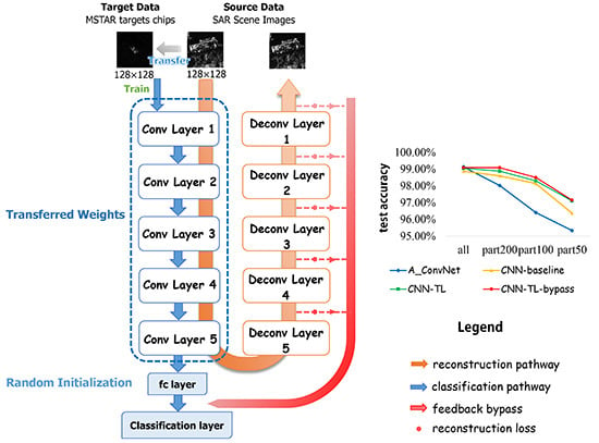
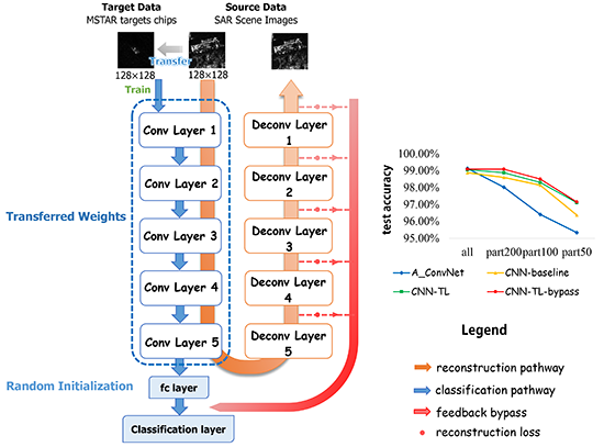
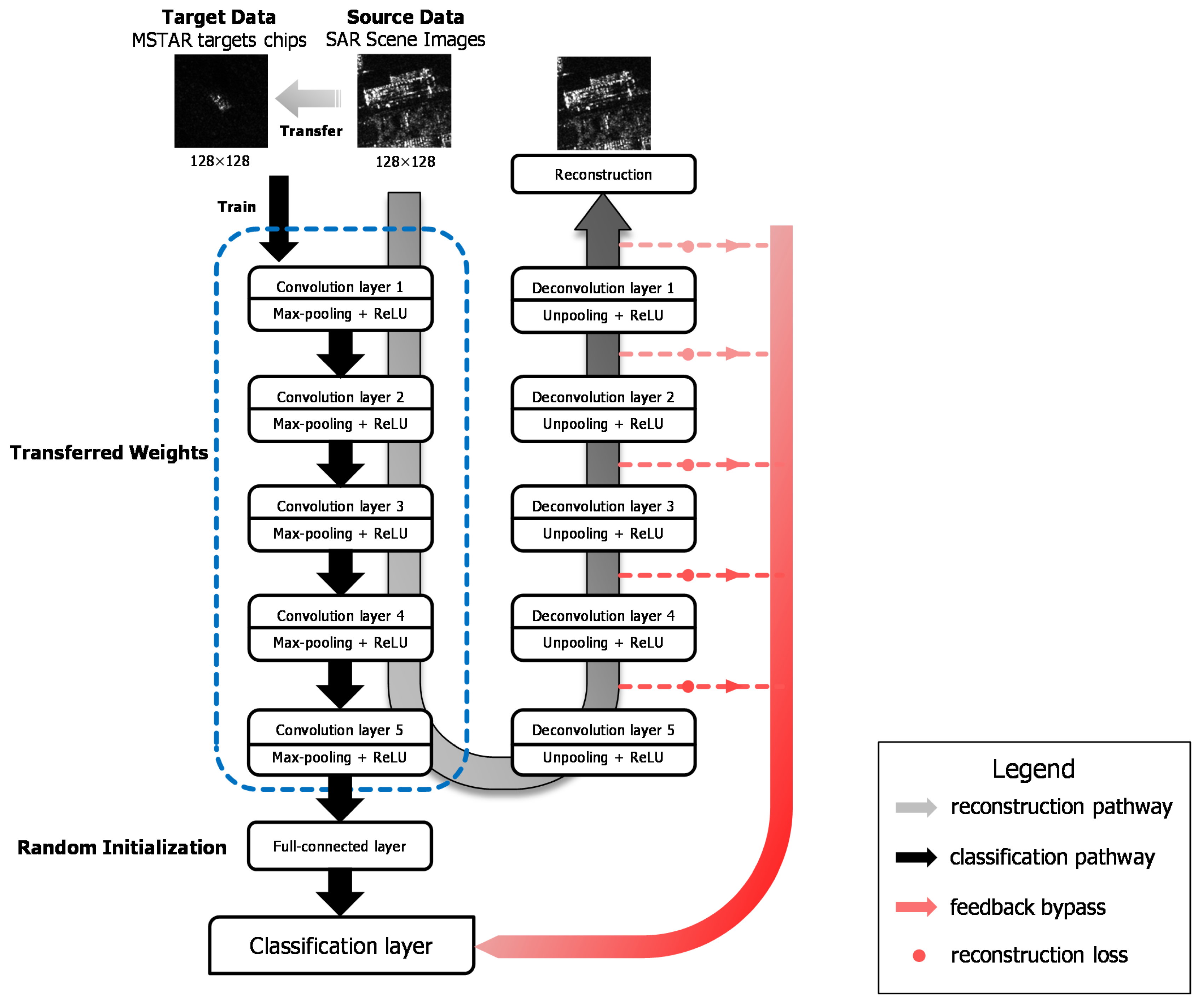
In order to accomplish the source and target tasks, we design an end-to-end assembled CNN architecture, integrating the reconstruction pathway, the classification pathway and the bypass to make the training process concise, as shown in Figure 1. The whole network can not only extract rich features of SAR scene images transferrable to SAR target dataset, but also perfectly reconstruct the input images, feeding back the reconstruction losses to classification pathway in order to preserve the information of input images.
Smith et al. [42] proposed the design pattern for deep CNNs, including increasing symmetry, pyramid shape and normalizing layer input, to help deep learning practitioners choose proper architectures for their tasks instead of being restricted to some existed architectures such as AlexNet. We design the assembled architecture based on the deep CNNs design pattern consequently. As depicted in Figure 1, the classification pathway of the architecture consists of five convolutional layers, followed by fully connected layers. The counterpart of each convolutional layer constitutes the decoding part in the reconstruction pathway and the bypass extended from every deconvolution layer with reconstruction loss is added to the classification layer. Specifically, our work adopts the pyramid structure, which means as the network goes deeper, the outputs of each layer are down-sampled by Max-pooling and the channel of the feature maps increase on the other hand. The number of the feature maps from the first convolution layer to the fifth convolution layer is shown in Table 1. Zero padding is added to preserve the spatial size of the input volume before the convolution operation. For each convolutional layer, a Max-pooling layer with size of 2 × 2 without overlapping is followed to reduce dimensions of the output feature maps and introduces a form of translation invariance. We explore two situations of the fully-connected layer (fc6), as shown in Table 1, either to preserve the 128-neuron fc layer or to cut off it. The output of the last fully-connected layer is fed to a 10-way Softmax classifier, which is a generalization of Logistic Regression to multiple classes, giving a probabilistic interpretation of each label. Rectifier Linear Units (ReLUs) are selected as the activation functions after each convolutional layer and fully-connected layer since ReLUs do not saturate and have high computational efficiency compared with the sigmoid function.
In terms of the reconstruction pathway, five unpooling and deconvolution layers are connected after the fifth convolutional layer in a cascade way to rebuild the input. Deconvolution layers implement transpose convolution operation, which is the reverse process of the convolution, serving as a decoding layer of the convolutional auto-encoder. The details will be elaborately explained in Section 3.2.
Additionally, the feedback bypass is attached in the architecture, which combines the reconstruction loss of each deconvolution layer in reconstruction pathway with the Softmax loss of the last fully-connected layer in classification pathway, aiming at improving the result of main target task. We will describe the details specifically in Section 3.3.
3.2. Unsupervised Learning on Source Task
To complete the source task with a large amount of unlabeled SAR data, an unsupervised learning method of stacked convolutional auto-encoders is applied in our work to train a hierarchical structure of several convolutional layers.
Each convolution layer is trained in a similar way and the individual unit is shown as Figure 2. For each two-dimensional feature map as the input of the unit, the encoding part decomposes it and the corresponding decoding part reconstructs it. In the lth layer’s training, there is the input with channels, that is, feature maps in 2-D arrays of , …, generating from the previous layer . The representation of the jth feature map in encoding part is given by
where and denote the jth kernel and bias of the lth layer, respectively. * represents the 2D convolution operation and f denotes the Rectified Linear Units . In order to maintain the size of feature maps after convolution, we use zero-paddings of where k denotes the kernel size.
In Max-pooling operation, we use the “what” and “where” method [40]. It means that the output of each Max-pooling layer contains “what” and “where” variables, preserving the values of Max-pooling results and the pooling switches, respectively. Instead of using fixed positions in unpooling operation, we record the locations of Max-pooling to maintain where the dominant features are located. With respect to the decoding part, the pooling switches variables together with the values are used to unpool the feature maps. Specifically speaking, the locations in Max-pooling are set as pooling values and the other positions are zero padding. The mathematical illustrations of Max-pooling and unpooling are given by
After unpooling the feature maps, the reconstruction is given by:
where Q denotes the kernels in deconvolution layers and indicates that the kernel Q is rotated 180 degrees; in other words, the matrix Q is flipped over both dimensions. Similar to the convolutional layers, the zero-padding of is utilized to maintain the size of feature maps.
Mean Square Error (MSE) is applied to measure the reconstruction loss; as a result, the loss function of the lth deconvolution layer to minimize is given by
where N denotes the size of each feature map of the th convolutional layer.
The set of parameters K, Q, b and c are learned via minimizing the loss function (3), completed by mini-batch stochastic gradient descent (SGD) with momentum and weight decay. The gradient of loss function with respect to each parameter is given by Equations (7)–(10):
where and denote the error term in the convolution and deconvolution layer, respectively. and can be related to which is the error term in the sampling layer. The relations among them are given by
where ⊙ denotes the Hadamard product. Then, the parameters can be updated with a proper learning rate , together with the momentum approach. The momentum parameter and the weight decay parameter are set as 0.9 and 0.005, respectively. Take K as an example:
where i is the iteration index and indicates the average partial derivative over the batch.
Since we train the SCAE in layer-wise fashion, the next convolution layer to be trained is stacked upon the previous adequately pre-trained layers as shown in Figure 3. The current layer receives the representation from the layers below as the input. When training the th convolution layer, the parameters of the 1th th layers are fixed and only the parameters of current layer are updated during the th layer training. In this way, a shallow network is trained every time a new layer is stacked, instead of updating the parameters from bottom to top.
3.3. Transferring Knowledge to Target Tasks
In our method, the reconstruction loss of SAR targets data is expected to be considered during classification. Consequently, the target tasks consist of the main part about recognition and the auxiliary part about reconstructing SAR targets.
In previous literature of transfer learning in CNN representation [43,44,45,46], CNN layers are proved to be transferrable from natural images to other medical data, such as neuroimaging data, ultrasound data and computed tomography (CT) images either using the off-the-shelf representations or fine-tuning the parameters. Despite the disparity between SAR scene images and SAR targets, the auxiliary target task is very similar to the source task, both of which focus on reconstruction. Knowledge used to transfer from the source task can be encoded into the feature representation, serving as the off-the-shelf features. By fixing the parameters in encoding part of reconstruction pathway, the decoding part is fine-tuned in a reducing learning rate with SAR targets.
In terms of the main target task of recognizing the different categories of SAR target data, which is very dissimilar to the source task, the classification pathway is designed, with two fully-connected layers concatenated after the encoding part of the reconstruction pathway. The convolutional layers are transferred from the pre-trained network and the rest of the classification pathway is randomly initialized. We fine-tune the transferred layers instead of freezing them to achieve a better performance. During the classification task, both the classification pathway and reconstruction pathway are activated, together with the bypass attached. The overall loss function contains two parts:
where refers to the loss in reconstruction pathway, denoted as
and denotes the cross-entropy loss between the label and the output of the last layer when using a Softmax classifier. The preserves the information of intermediate layers, acting as a regularizer during supervised training, which prevents over-fitting and gradient vanishing. Different values of can be experienced to control the influence of each layer.
4. Experiments and Discussions
To evaluate the proposed method, we set the experiments as the following. Firstly, a brief introduction of datasets is given in Section 4.1 and the training procedure of the proposed method is illustrated in Section 4.2. After that, we train the classification pathway from scratch with SAR targets as our baseline, as shown in Section 4.3. To estimate the effectiveness of transfer learning, we compare the results between the baseline and the proposed method in different aspects, shown in Section 4.4. In addition, Section 4.5 explores different sizes of training datasets on our method, compared with the baseline and one of the state-of-the-art methods.
4.1. Materials
4.1.1. Source Domain Dataset
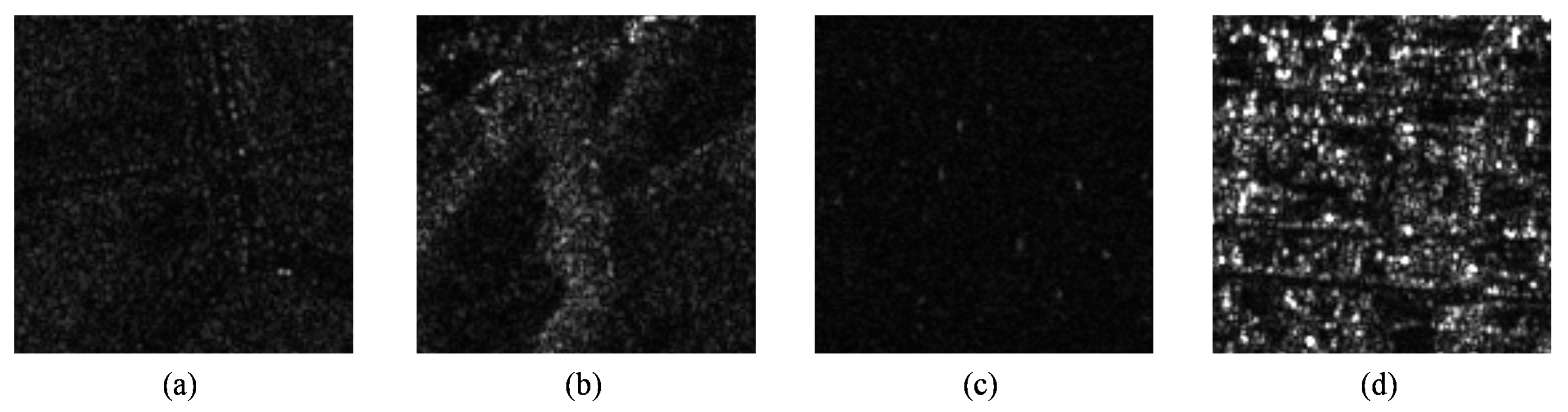
A large number of unlabeled SAR scene images are utilized to perform as the source domain. These images are collected by TerraSAR-X, a German Earth-observation satellite that provides high-quality and precise Earth observation data of 3 m resolution with StripMap mode. We select the areas covering various landscapes such as cities, forests, mountains and cultivated lands and crop them into 128 × 128 pixels with overlap, as shown in Figure 4. The number of SAR scene images is up to 50,000.
4.1.2. Target Domain Dataset
In the target domain, we employ the Moving and Stationary Target Acquisition and Recognition (MSTAR) public release dataset in our work [47]. MSTAR dataset, collected by Sandia National Laboratory SAR sensor platform, is extensively used in the research of SAR automatic target recognition for algorithm development. The dataset contains 10 categories of military vehicles: the T72, BTR70, BMP2, 2S1, BRDM2, BTR60, D7, T62, ZIL131 and ZSU23, with the resolution of 1-ft on X-band. Those images are acquired at depression angles of and , serving as the testing dataset and the training dataset, respectively, and the aspect angle covers in the range of to . Details of MSTAR dataset for experiment are shown in Table 2. It is a practical approach to make data augmentation for the purpose of improving the performance of training CNNs. Therefore, we augment the MSTAR dataset with translation and mirroring by ten times.
4.2. Training Procedure of Transfer Learning Based Method
- 1.
- Pre-train Reconstruction Pathway with SAR Scene ImagesAs is elaborated in Section 3, we train the reconstruction pathway using stacked convolutional auto-encoders with pooling-switches in layer-wise fashion on unlabeled SAR scene dataset.
- 2.
- Transfer Learning to Target Tasks
- Classification Pathway TransferredIn this part, we froze the decoding part of reconstruction pathway and reuse the encoding layers to train the classification pathway with MSTAR dataset. The learning rate of five convolutional layers are reduced to a small value compare with the full-connected layers, which are Gaussian randomly initialized.
- Reconstruction Pathway TransferredFor the auxiliary target task, we froze the classification pathway and only fine-tune the decoding part with a reduced learning rate with MSTAR dataset regardless the categories.
- 3.
- Fine-Tune the Assembled Network with Bypass ActivatedFinally, we activate all the pathways and joint the reconstruction loss to the classification pathway. We fine-tune the whole network by adjusting the loss weight of each reconstruction layer to an appropriate value.
4.3. Baseline: Training the Assembled CNN with MSTAR from Scratch
In this subsection, we only use MSTAR dataset to train the network from scratch as our baseline. More specifically, to complete the primary target task and the auxiliary target task, the classification and the reconstruction pathway are trained separately. We initialize the weight parameters of each layer randomly from Gaussian distributions of zero mean and a standard deviation of where n denotes the number of the input neuron. This initialization method ensures that all neurons in the network initially have approximately the same output distribution and empirically improves the rate of convergence. The details about the parameters initialization of the classification pathway are shown as Table 3, similar to the reconstruction pathway.
We train the network using mini-batch SGD, with an initial learning rate of 0.01 and a reducing factor of 0.1 after 2000 iterations. The momentum parameter is set to 0.9 and the weight decay parameter 0.005. The result of the classification task is shown in Table 4, reaching an average accuracy of 98.3%. We select an image from test dataset to evaluate the training result of reconstruction pathway. Table 5 records the MSE loss of the image and the reconstruction signal after each convolution layer being trained. Figure 5 and Figure 6 show the reconstructed image and the learned kernels of each convolutional layer respectively.
4.4. Transfer Learning: from Source Task to Target Tasks
Transfer learning is applied to both primary target task (10-class MSTAR recognition) and auxiliary target task (reconstructing MSTAR dataset). We firstly concentrate on the source task to train the reconstruction pathway, following the training procedure in Section 4.2. The reconstruction results are shown in Figure 7.
4.4.1. Auxiliary Target Task
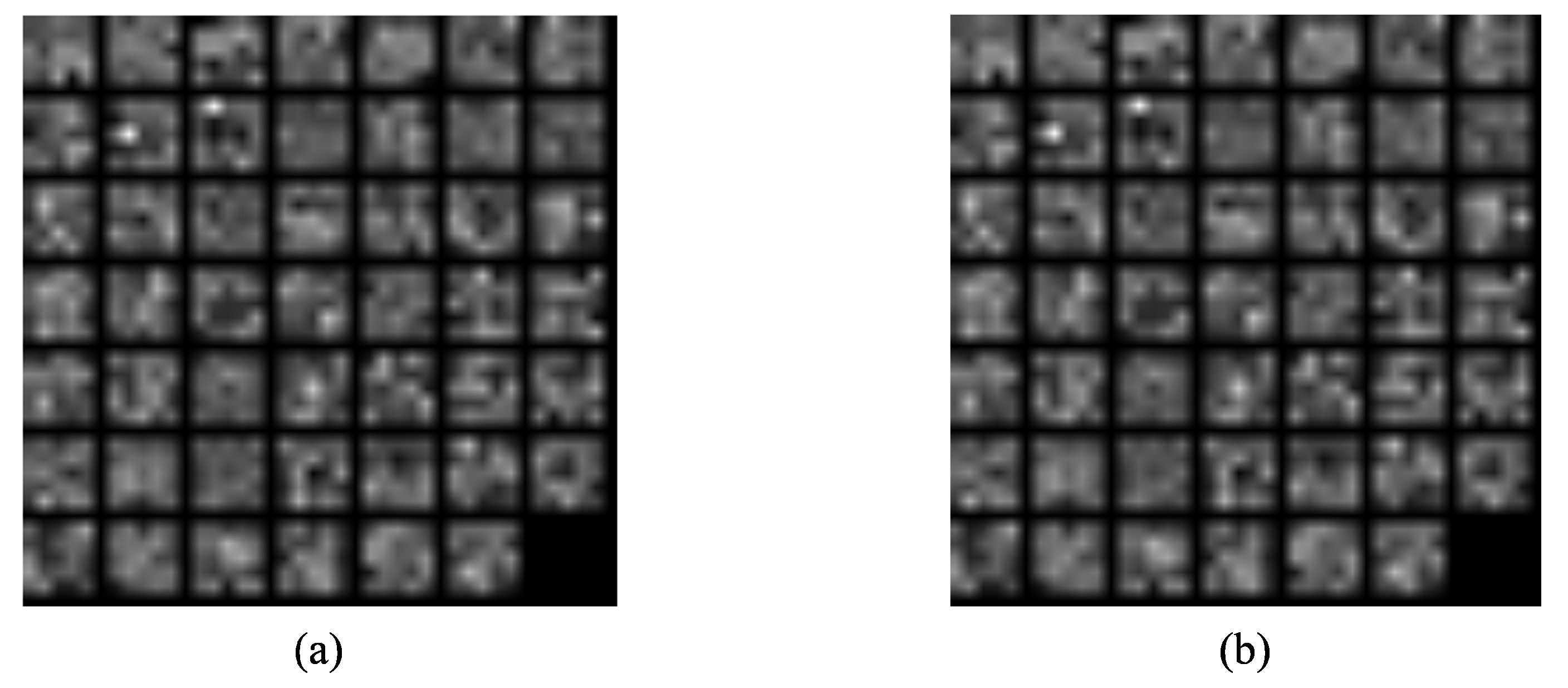
In this part, we firstly attempt to fine-tune all the layers in reconstruction pathway with MSTAR dataset on pre-trained network. The variation of L2 norm of each kernel is computed to estimate the changes during transfer learning. The changes of convolutional kernels in each layer are analyzed in Table 6 and the convolutional kernels in the first layer before and after transfer learning are shown in Figure 8. The phenomenon can be observed that the convolution kernels are barely changed during the transfer learning from source task to auxiliary target task, both of which focus on keeping good reconstruction of the input. As a result, we can use the off-the-shelf representations of the pre-trained network, extracting features from the convolutional layers directly and fine-tuning the decoding part only to reduce the training time.
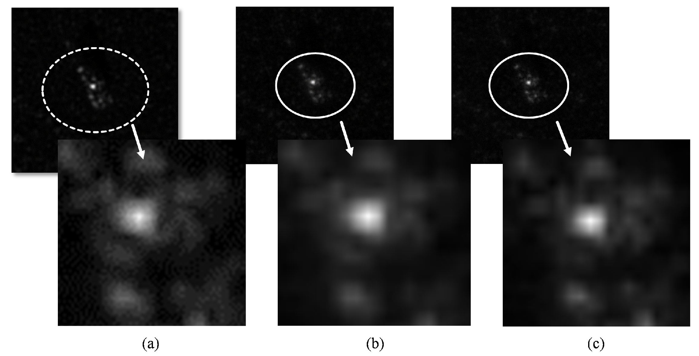
When training the reconstruction pathway in layer-wise fashion only with MSTAR dataset from scratch, the reconstruction loss of the input layer is while the transfer learning method can reduce the result to . We take an image of MSTAR testing dataset as visualization shown in Figure 9, indicating that the transfer learning based method can reconstruct more details in the reconstructing images.
4.4.2. Primary Target Task
The classification results of transfer learning based method are recorded in Table 7. The confusion matrix is shown in the table, indicating the recognition accuracy of each category. Compared with the result in Table 4, it is obvious that the transfer learning method improves the recognition rate of 10-class SAR vehicle targets, achieving an improvement with 0.75%.
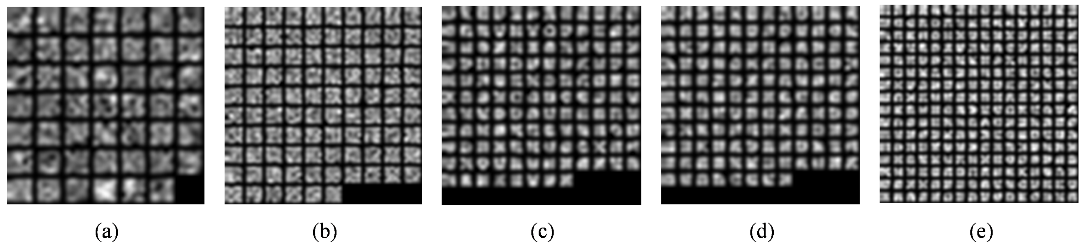
In addition, variations of convolution kernels are observed during primary target task transfer learning. The kernel numbers of each convolutional layer, which changed over 40% in L2-norms, are recorded in Table 8 and kernel visualizations of the first and the third convolutional layer are shown in Figure 10. From Table 8, we can see that a majority of kernels have significantly changed (over 30% in -norm) in the first convolution layer, while the last several layers show little change. This can be validated in Figure 10 as well. Among them, the first convolutional layer has the highest variation than other four layers, which is similar to the auxiliary target task. Furthermore, it can be observed that the convolution kernels of each layer in auxiliary target task have minuscule change compared with the primary target task. This is possibly due to the dissimilarity degree of two tasks. Both the source task and the auxiliary target task aim at encoding the input and reconstructing perfectly as far as possible, while the primary target task focus on classification, which is more dissimilar to the source task. Thus, instead of using off-the-shelf feature representations in auxiliary target task, we fine-tune all the convolutional layers in classification pathways to achieve a better performance.
After adding the bypass to the classification pathway, the final classification accuracy achieves 99.09% on average, which brings about a minor improvement of 0.04%, compared to the 0.17% change transfer learning makes. Figure 11 shows the loss curve of test dataset during training, illustrating the benefit of bypass. The test loss converges at the later stage of transfer learning and vibrates in a small range as shown in (a). After that, training the current network with the attached bypass enables the loss to decrease again as shown in (b). The attached bypass makes a further effort to improve the performance, maintaining the high recognition rate in the case of cutting down the training number to 200 per class specifically (see Section 4.5).
According to Table 1, we have explored two different architectures, with and without the 128-neuron fc layer, in order to evaluate our method. The result shows that adding the optional fully-connected layer improves the recognition rate from 98.5 to 99.05%, which indicates that it seems to be inappropriate to cut off the fully-connected layer blindly to avoid overfitting in the case of limited training data, as it plays an efficient role in developing more abstraction and high-level features, beneficial to classification.
4.5. The Effectiveness of Transfer Learning
In Figure 12, we compare the recognition results of our transfer learning based method (CNN-TL-bypass) with the conventional approach (SVM) and some state-of-the-art SAR recognition methods in recent years. It is 8.67%, 5.43%, 5.68%, 2.85%, 4.09% better than SVM, sparse representation of monogenic signal (MSRC) [18], tri-task joint sparse representation (TJSR) [48], supervised discriminative dictionary learning and sparse representation (SDDLSR) [8] and joint dynamic sparse representation (JDSR) [49]. In addition, our method can achieve a comparable performance to the state-of-the-art methods based on deep learning (A-ConvNet [24] and DCHUN [50]), shown in Figure 12. In order to verify the advantage of our method for a further step, experiments have been conducted on different sizes of training dataset. By randomly selecting 200, 100, 50 samples in each category of MSTAR training set as the training samples, respectively, we experiment with the A-ConvNet method [24], the baseline (written as CNN-baseline), and the proposed method without bypass (written as CNN-TL) and proposed method with bypass (written as CNN-TL-bypass). The recognition rate of each method is shown in Figure 13.
To illustrate the results precisely, we replicate the experiment of [24] and obtain an accuracy of 98.51%, which is lower than what the literature proposed, probably due to the different experiment settings. Although the A-ConvNet achieves extraordinary success in recognizing a 10-class MSTAR dataset, according to whether the literature (99.13%) or our replication (98.51%), the performance fiercely deteriorates when reducing the training data, similar to results of the CNN-baseline of which the network is trained with the MSTAR dataset from scratch as well. In contrast, the transfer learning based method decreases the tendency of dramatic deterioration. Compared to 98.02% (part-200), 96.04% (part-100) and 95.34% (part-50) for the state-of-the-art deep learning based approach (A-ConvNet) [24] in SAR ATR, our method achieves 1.07%, 2.11% and 1.79% better results. Transfer learning is 0.17%, 0.28%, 0.16% and 0.74% better than baseline with full training dataset, part-200 dataset, part-100 dataset and part-50 dataset, respectively. According to [50], their network can achieve an accuracy of 94.97% when using about 30% training data to train it. In our work, however, the accuracy can reach 97.15% with less than 20% training data (part-50), which has a superiority of 2.18% compared with [50].
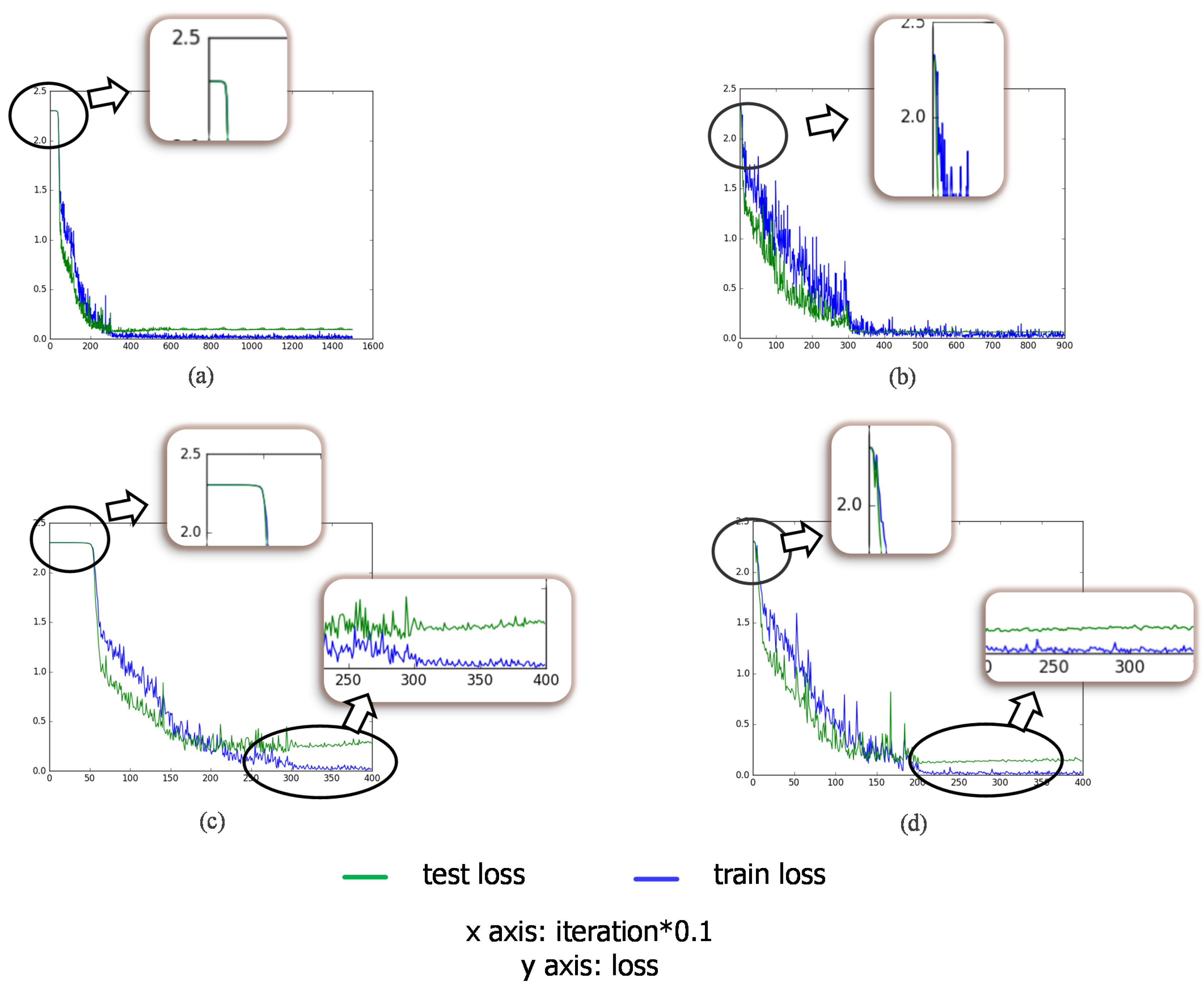
By analyzing the loss curve under different experiment setups shown in Figure 14, we find that transfer learning makes the gradients drop faster than those in baseline case in which the network is trained from scratch, obviously appeared with a smaller training dataset. Moreover, the proposed method is effective at avoiding over-fitting to some degree, narrowing the gap between training and testing loss (or accuracy), preventing the model performance on testing dataset from getting worse.
In our work, the abundant unlabeled SAR scene images are chosen as our source data to pre-train the network transferred to the SAR classification task, instead of the ImageNet dataset, which is widely adopted in previous studies. AlexNet [19] trained on ImageNet, by contract, is experimented to transfer the five convolutional layers to our target task (written as AlexNet-ImageNet-TL). For the full training dataset, the AlexNet-ImageNet-TL achieves 96.62% on 10-class classification of MSTAR, as shown in Table 9. As the training dataset of target task decreases to part-200, part-100 and part-50, the accuracies drop to 96.16%, 95.75% and 93.48%, which are 2.93%, 2.75% and 3.67% lower than CNN-TL-bypass, respectively, shown in Figure 13. Thus, it can be seen that SAR scene images are more appropriate than optical images in transfer learning to solve the SAR target recognition problem for the similarity between the source data and the target data.
5. Conclusions
For the purpose of overcoming the difficulties of training a deep CNN resulting from limited SAR target images, we proposed a transfer learning based method to transfer knowledge learned from a large amount of unlabeled SAR scene data to SAR target recognition tasks and feedback to the reconstruction loss to the classification pathway. Our method is competitive both with the state-of-the-art methods based on CNNs and the conventional approaches on MSTAR dataset recognition when using all training samples, and achieves superior performance than that when experimenting on a smaller size of training data. The result reveals that transfer learning is an effective way to solve the data hungry problem and knowledge learned from unlabeled SAR scene images is transferrable both on SAR target classification and reconstruction task. What to transfer and how to transfer are important issues in transfer learning. Choosing an appropriate source dataset and whether to use the off-the-shelf representations or to fine-tune the parameters should be deliberated. In addition, considering the reconstruction loss is beneficial for improving the classification performance to some degree.
Acknowledgments
This work was supported by the National Natural Science Foundation of China (Grant No. 61331017 and No. 61701478.)
Author Contributions
Zhongling Huang and Zongxu Pan conceived and designed the experiments; Zhongling Huang performed the experiments; Zhongling Huang analyzed the data; Bin Lei and Zongxu Pan contributed materials and computing resources; Zhongling Huang and Zongxu Pan wrote the paper.
Conflicts of Interest
The authors declare no conflict of interest.
References
- El-Darymli, K.; Gill, E.W.; McGuire, P.; Power, D.; Moloney, C. Automatic Target Recognition in Synthetic Aperture Radar Imagery: A State-of-the-Art Review. IEEE Access 2016, 4, 6014–6058. [Google Scholar] [CrossRef]
- Zhang, H.; Nasrabadi, N.M.; Zhang, Y.; Huang, T.S. Multi-View Automatic Target Recognition using Joint Sparse Representation. IEEE Trans. Aerosp. Electron. Syst. 2012, 48, 2481–2497. [Google Scholar] [CrossRef]
- Mehra, R.K.; Huff, M.; Ravichandran, B.; Williams, A.C. Non-Parametric Error Estimation Techniques Applied to MSTAR Data Sets. In Proceedings of the SPIE, Orlando, FL, USA, 15 September 1998; pp. 614–624. [Google Scholar]
- Novak, L.M.; Owirka, G.J.; Brower, W.S. Performance of 10- and 20-Target MSE Classifiers. IEEE Trans. Aerosp. Electron. Syst. 2000, 36, 1279–1289. [Google Scholar]
- Saghri, J.A. SAR Automatic Target Recognition using Maximum Likelihood Template-based Classifiers. In Proceedings of the SPIE, San Diego, CA, USA, 15 September 2008; Volume 7073. [Google Scholar]
- Anagnostopoulos, G.C. SVM-Based Target Recognition From Synthetic Aperture Radar Images using Target Region Outline Descriptors. Nonlinear Anal. Theory Methods Appl. 2009, 71, 2934–2939. [Google Scholar] [CrossRef]
- Dong, G.; Kuang, G. SAR Target Recognition Via Sparse Representation of Monogenic Signal on Grassmann Manifolds. IEEE J. Sel. Top. Appl. Earth Obs. Remote Sens. 2016, 9, 1308–1319. [Google Scholar] [CrossRef]
- Song, S.; Xu, B.; Yang, J. SAR Target Recognition via Supervised Discriminative Dictionary Learning and Sparse Representation of the SAR-HOG Feature. Remote Sens. 2016, 8, 683. [Google Scholar] [CrossRef]
- Cheng, J.; Li, L.; Li, H.; Wang, F. SAR Target Recognition Based on Improved Joint Sparse Representation. EURASIP J. Adv. Signal Process. 2014, 2014, 87. [Google Scholar] [CrossRef]
- Pan, Z.; Qiu, X.; Huang, Z.; Lei, B. Airplane Recognition in TerraSAR-X Images via Scatter Cluster Extraction and Reweighted Sparse Representation. IEEE Geosci. Remote Sens. Lett. 2017, 14, 112–116. [Google Scholar] [CrossRef]
- Yu, X.; Li, Y.; Jiao, L.C. SAR Automatic Target Recognition Based on Classifiers Fusion. In Proceedings of the International Workshop on Multi-Platform/multi-Sensor Remote Sensing and Mapping, Xiamen, China, 10–12 January 2011; pp. 1–5. [Google Scholar]
- Liu, H.; Li, S. Decision Fusion of Sparse Representation and Support Vector Machine for SAR Image Target recognition. Neurocomputing 2013, 113, 97–104. [Google Scholar] [CrossRef]
- Rogers, S.K.; Colombi, J.M.; Martin, C.E.; Gainey, J.C.; Fielding, K.H.; Burns, T.J.; Ruck, D.W.; Kabrisky, M.; Oxley, M. Neural networks for automatic target recognition. Neural Netw. 1995, 8, 1153–1184. [Google Scholar] [CrossRef]
- Novak, L.M.; Owirka, G.J.; Brower, W.S. An Efficient Multi-Target SAR ATR ASlgorithm. In Proceedings of the Asilomar Conference on Signals, Systems and Computers (Cat. No. 98CH36284), Pacific Grove, CA, USA, 1–4 November 2002; Volume1, pp. 3–13. [Google Scholar]
- Zhang, X.; Qin, J.; Li, G. SAR Target Classification using Bayesian Compressive Sensing with Scattering Centers Features. Prog. Electromagn. Res. 2013, 136, 385–407. [Google Scholar] [CrossRef]
- Ruan, H.; Zhang, R.; Li, J.; Zhan, Y. SAR Target Classification Based on Multiscale Sparse Representation. In Proceedings of the International Society for Optics and Photonics, Xiamen, China, 2 March 2016; Volume 9901. [Google Scholar]
- Srinivas, U.; Monga, V.; Raj, R.G. SAR Automatic Target Recognition using Discriminative Graphical Models. IEEE Trans. Aerosp. Electron. Syst. 2014, 50, 591–606. [Google Scholar] [CrossRef]
- Dong, G.; Wang, N.; Kuang, G. Sparse Representation of Monogenic Signal: With Application to Target Recognition in SAR Images. IEEE Signal Process. Lett. 2014, 21, 952–956. [Google Scholar]
- Krizhevsky, A.; Sutskever, I.; Hinton, G.E. Imagenet Classification with Deep Convolutional Neural Networks. In Proceedings of the Neural Information Processing System (NIPS), Harrahs and Harveys, Lake Tahoe, NV, USA, 3–8 December 2012; Volume 2, pp. 1097–1105. [Google Scholar]
- Simonyan, K.; Zisserman, A. Very Deep Convolutional Networks for Large-Scale Image Recognition. arXiv, 2014; arXiv:1409.1556. [Google Scholar]
- Szegedy, C.; Liu, W.; Jia, Y.; Sermanet, P.; Reed, S.; Anguelov, D.; Erhan, D.; Vanhoucke, V.; Rabinovich, A. Going Deeper with Convolutions. In Proceedings of the IEEE Conference on Computer Vision and Pattern Recognition, Boston, MA, USA, 7–12 June 2015; pp. 1–9. [Google Scholar]
- He, K.; Zhang, X.; Ren, S.; Sun, J. Deep Residual Learning for Image Recognition. In Proceedings of the 2016 IEEE Conference on Computer Vision and Pattern Recognition (CVPR), Las Vegas, NV, USA, 27–30 June 2016; pp. 770–778. [Google Scholar]
- Ding, J.; Chen, B.; Liu, H.; Huang, M. Convolutional Neural Network with Data Augmentation for SAR Target Recognition. IEEE Geosci. Remote Sens. Lett. 2016, 13, 364–368. [Google Scholar] [CrossRef]
- Chen, S.; Wang, H.; Xu, F.; Jin, Y.Q. Target Classification using the Deep Convolutional Networks for SAR Images. IEEE Trans. Geosci. Remote Sens. 2016, 54, 4806–4817. [Google Scholar] [CrossRef]
- Yosinski, J.; Clune, J.; Bengio, Y.; Lipson, H. How Transferable Are Features in Deep Neural Networks? In Proceedings of the 27th International Conference on Neural Information Processing Systems, Montreal, QC, Canada, 8–13 December 2014; pp. 3320–3328. [Google Scholar]
- Nanni, L.; Ghidoni, S. How Could a Subcellular Image, or a Painting by Van Gogh, Be Similar to a Great White Shark or to a Pizza? Pattern Recognit. Lett. 2017, 85, 1–7. [Google Scholar] [CrossRef]
- Nanni, L.; Ghidoni, S.; Brahnam, S. Handcrafted vs. Non-Handcrafted Features for Computer Vision Classification. Pattern Recognit. 2017, 71, 158–172. [Google Scholar] [CrossRef]
- Akçay, S.; Kundegorski, M.E.; Devereux, M.; Breckon, T.P. Transfer Learning using Convolutional Neural Networks for Object Classification within X-ray Baggage Security Imagery. In Proceedings of the 2016 IEEE International Conference on Image Processing (ICIP), Phoenix, AZ, USA, 25–28 September 2016; pp. 1057–1061. [Google Scholar]
- Oquab, M.; Bottou, L.; Laptev, I.; Sivic, J. Learning and Transferring Mid-Level Image Representations Using Convolutional Neural Networks. In Proceedings of the 2014 IEEE Conference on Computer Vision and Pattern Recognition, Columbus, OH, USA, 23–28 June 2014; pp. 1717–1724. [Google Scholar]
- Chen, S.; Wang, H. SAR Target Recognition Based on Deep Learning. In Proceedings of the 2014 International Conference on Data Science and Advanced Analytics (DSAA), Shanghai, China, 30 October–1 November 2014; pp. 541–547. [Google Scholar]
- Morgan, D.A. Deep Convolutional Neural Networks for ATR from SAR Imagery. In Proceedings of the Algorithms for Synthetic Aperture Radar Imagery XXII, Baltimore, MD, USA; 2015. [Google Scholar]
- Wilmanski, M.; Kreucher, C.; Lauer, J. Modern Approaches in Deep Learning for SAR ATR. Int. Soc. Opt. Photonics 2016, 9843, 98430N. [Google Scholar]
- Pan, S.J.; Yang, Q. A Survey on Transfer Learning. IEEE Trans. Knowl. Data Eng. 2010, 22, 1345–1359. [Google Scholar] [CrossRef]
- Shin, H.; Roth, H.R.; Gao, M.; Lu, L.; Xu, Z.; Nogues, I.; Yao, J.; Mollura, D.J.; Summers, R.M. Deep Convolutional Neural Networks for Computer-Aided Detection: CNN Architectures, Dataset Characteristics and Transfer Learning. IEEE Trans. Med. Image 2016, 35, 1285–1298. [Google Scholar] [CrossRef] [PubMed]
- Christodoulidis, S.; Anthimopoulos, M.; Ebner, L.; Christe, A.; Mougiakakou, S. Multisource Transfer Learning With Convolutional Neural Networks for Lung Pattern Analysis. IEEE J. Biomed. Health Inform. 2017, 21, 76–84. [Google Scholar] [CrossRef] [PubMed]
- Ravishankar, H.; Sudhakar, P.; Venkataramani, R.; Thiruvenkadam, S.; Annangi, P.; Babu, N.; Vaidya, V. Understanding the Mechanisms of Deep Transfer Learning for Medical Images. In Deep Learning and Data Labeling for Medical Applications: First International Workshop, LABELS 2016, and Second International Workshop, DLMIA 2016, Held in Conjunction with MICCAI 2016, Athens, Greece, October 21, 2016, Proceedings; Springer International Publishing: Cham, Switzerland, 2016; pp. 188–196. [Google Scholar]
- Masci, J.; Meier, U.; Cireşan, D.; Schmidhuber, J. Stacked Convolutional Auto-Encoders for Hierarchical Feature Extraction. In Artificial Neural Networks and Machine Learning – ICANN 2011: 21st International Conference on Artificial Neural Networks, Espoo, Finland, June 14-17, 2011, Proceedings, Part I; Springer-Verlag: Heidelberg, Germany, 2011; pp. 52–59. [Google Scholar]
- Glorot, X.; Bordes, A.; Bengio, Y. Deep Sparse Rectifier Neural Networks. In Proceedings of the Fourteenth International Conference on Artificial Intelligence and Statistics, Ft. Lauderdale, FL, USA, 11–13 April 2011; Volume 15, pp. 315–323. [Google Scholar]
- Paine, T.L.; Khorrami, P.; Han, W.; Huang, T.S. An Analysis of Unsupervised Pre-training in Light of Recent Advances. arXiv, 2014; arXiv:1412.6597. [Google Scholar]
- Zhao, J.; Mathieu, M.; Goroshin, R.; Lecun, Y. Stacked What-Where Auto-encoders. arXiv, 2015; arXiv:1506.02351. [Google Scholar]
- Zhang, Y.; Lee, K.; Lee, H.; EDU, U. Augmenting Supervised Neural Networks with Unsupervised Objectives for Large-Scale Image classification. Proceedings of Machine Learning Research, New York, NY, USA, 20–22 June 2016; Volume 48, pp. 612–621. [Google Scholar]
- Smith, L.N.; Topin, N. Deep Convolutional Neural Network Design Patterns. arXiv, 2016; arXiv:1611.00847. [Google Scholar]
- Gupta, S.; Girshick, R.; Arbelaez, P.; Malik, J. Learning Rich Features from RGB-D Images for Object Detection and Segmentation. In European Conference on Computer Vision; Springer: Cham, Switzerland, 2014; pp. 345–360. [Google Scholar]
- Gupta, S.; Arbelaez, P.; Girshick, R.; Malik, J. Indoor Scene Understanding with RGB-D Images: Bottom-up Segmentation, Object Detection and Semantic Segmentation. Int. J. Comput. Vis. 2015, 112, 133–149. [Google Scholar] [CrossRef]
- Gupta, A.; Ayhan, M.S.; Maida, A.S. Natural Image Bases to Represent Neuroimaging Data. Int. Conf. Mach. Learn. 2013, 987–994. [Google Scholar]
- Chen, H.; Dou, Q.; Ni, D.; Cheng, J.; Qin, J.; Li, S.; Heng, P. Automatic Fetal Ultrasound Standard Plane Detection using Knowledge Transferred Recurrent Neural Networks. Med. Image Comput. Comput. Assist. Interv. 2015, 9349, 507–514. [Google Scholar]
- The Air Force Moving and Stationary Target Recognition Database. Available online: https://www.sdms.afrl.af.mil/datasets/mstar/ (accessed on 3 February 2016).
- Dong, G.; Kuang, G.; Wang, N.; Zhao, L.; Lu, J. SAR Target Recognition via Joint Sparse Representation of Monogenic Signal. IEEE J. Sel. Top. Appl. Earth Obs. Remote Sens. 2015, 8, 3316–3328. [Google Scholar] [CrossRef]
- Sun, Y.; Du, L.; Wang, Y.; Wang, Y.; Hu, J. SAR Automatic Target Recognition Based on Dictionary Learning and Joint Dynamic Sparse Representation. IEEE Geosci. Remote Sens. Lett. 2016, 13, 1777–1781. [Google Scholar] [CrossRef]
- Lin, Z.; Ji, K.; Kang, M.; Leng, X.; Zou, H. Deep Convolutional Highway Unit Network for SAR Target Classification with Limited Labeled Training Data. IEEE Geosci. Remote Sens. Lett. 2017, 14, 1091–1095. [Google Scholar] [CrossRef]
Figure 1.
Assembled CNN Architecture.

Figure 2.
One-layer convolutional auto-encoder.
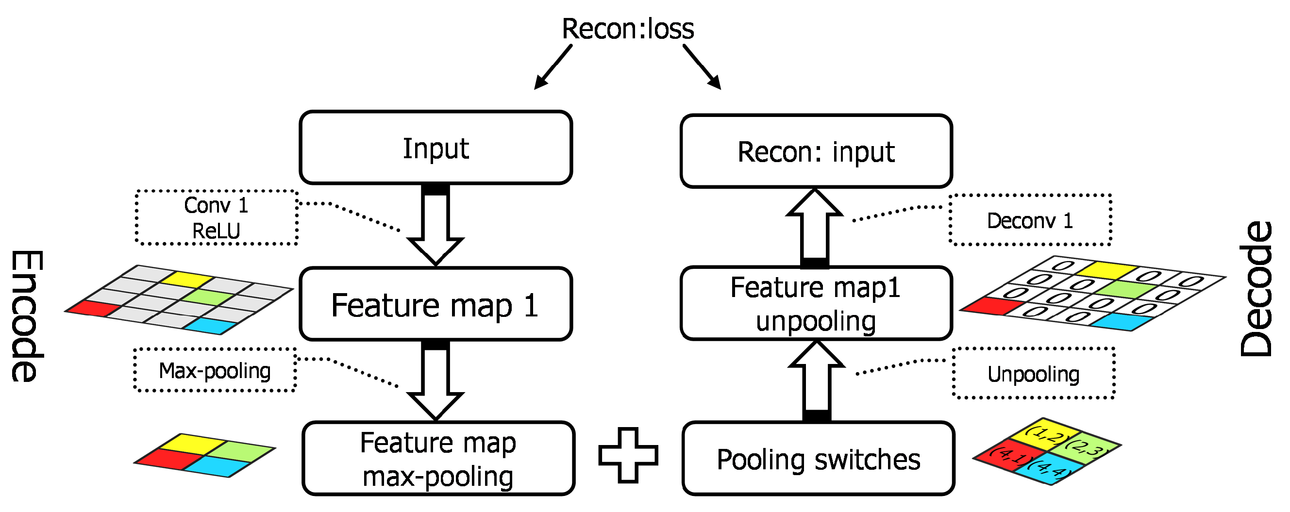
Figure 3.
Stacked convolutional auto-encoders in layer-wise fashion for the second layer.
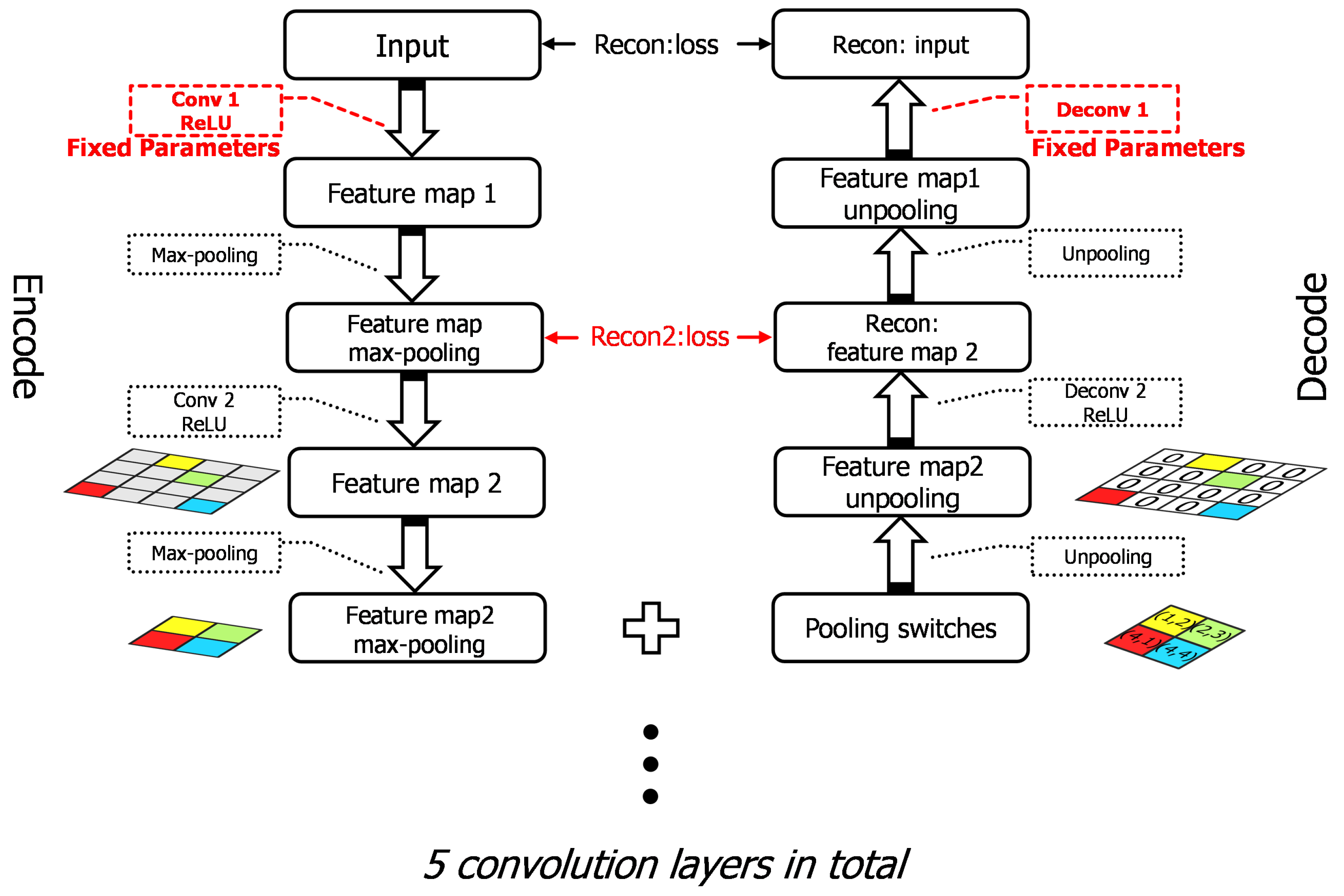
Figure 4.
Different types of SAR scene images. (a) cultivated lands; (b) mountains; (c) rivers; (d) cities.
Figure 4.
Different types of SAR scene images. (a) cultivated lands; (b) mountains; (c) rivers; (d) cities.

Figure 5.
Training results of reconstruction pathway (baseline). (a) the input image; (b–f) the reconstruction images of five convolutional layers.
Figure 5.
Training results of reconstruction pathway (baseline). (a) the input image; (b–f) the reconstruction images of five convolutional layers.
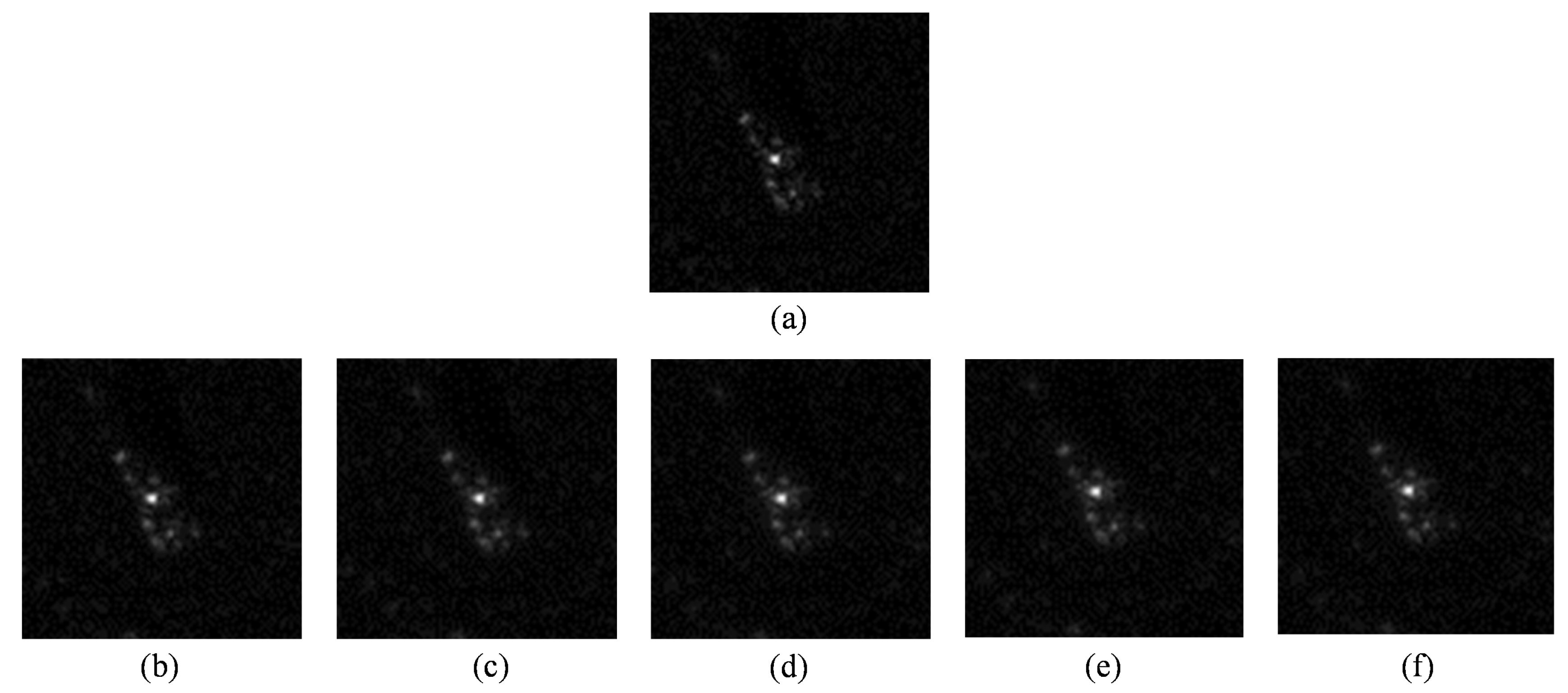
Figure 6.
Training results of reconstruction pathway (baseline). (a–e) the kernels of convolutional layers 1–5, respectively.
Figure 6.
Training results of reconstruction pathway (baseline). (a–e) the kernels of convolutional layers 1–5, respectively.

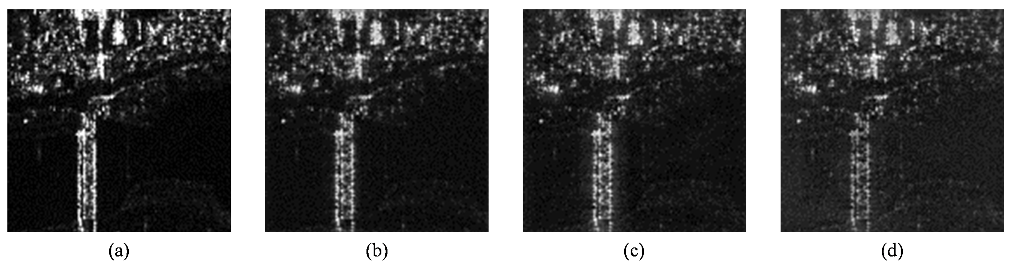
Figure 7.
Training results of reconstruction pathway (source task). (a) the input image; (b–d) the reconstruction images of the 1st, 3rd, and 5th convolutional layer, respectively.
Figure 7.
Training results of reconstruction pathway (source task). (a) the input image; (b–d) the reconstruction images of the 1st, 3rd, and 5th convolutional layer, respectively.

Figure 8.
The 1st convolutional layer kernels of baseline and transfer learning method. (a) baseline; (b) transfer learning method.
Figure 8.
The 1st convolutional layer kernels of baseline and transfer learning method. (a) baseline; (b) transfer learning method.

Figure 9.
Reconstruction comparison between baseline and transfer learning. (a) input image; (b) reconstruction image of SCAE training from scratch; (c) reconstruction image of transfer learning.
Figure 9.
Reconstruction comparison between baseline and transfer learning. (a) input image; (b) reconstruction image of SCAE training from scratch; (c) reconstruction image of transfer learning.

Figure 10.
Convolutional layer kernels of baseline and transfer learning. (a,b) the kernels in the 1st convolutional layer before and after transfer learning; (c,d) the kernels in the 3rd convolutional layer before and after transfer learning.
Figure 10.
Convolutional layer kernels of baseline and transfer learning. (a,b) the kernels in the 1st convolutional layer before and after transfer learning; (c,d) the kernels in the 3rd convolutional layer before and after transfer learning.
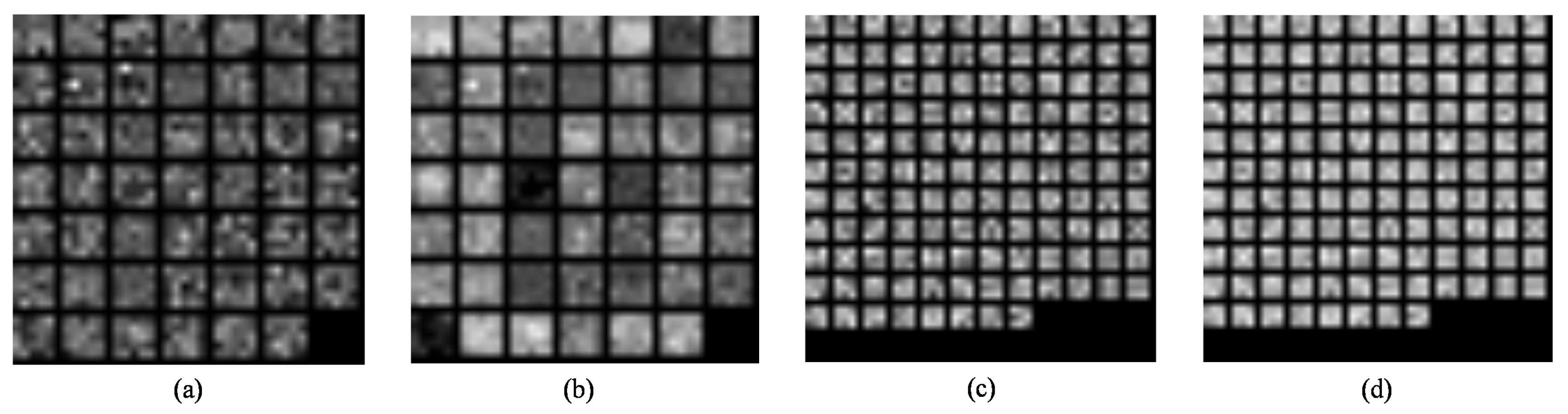
Figure 11.
Testing loss curve during training. (a) the testing curve during transfer learning; (b) the testing curve after attaching the bypass.
Figure 11.
Testing loss curve during training. (a) the testing curve during transfer learning; (b) the testing curve after attaching the bypass.
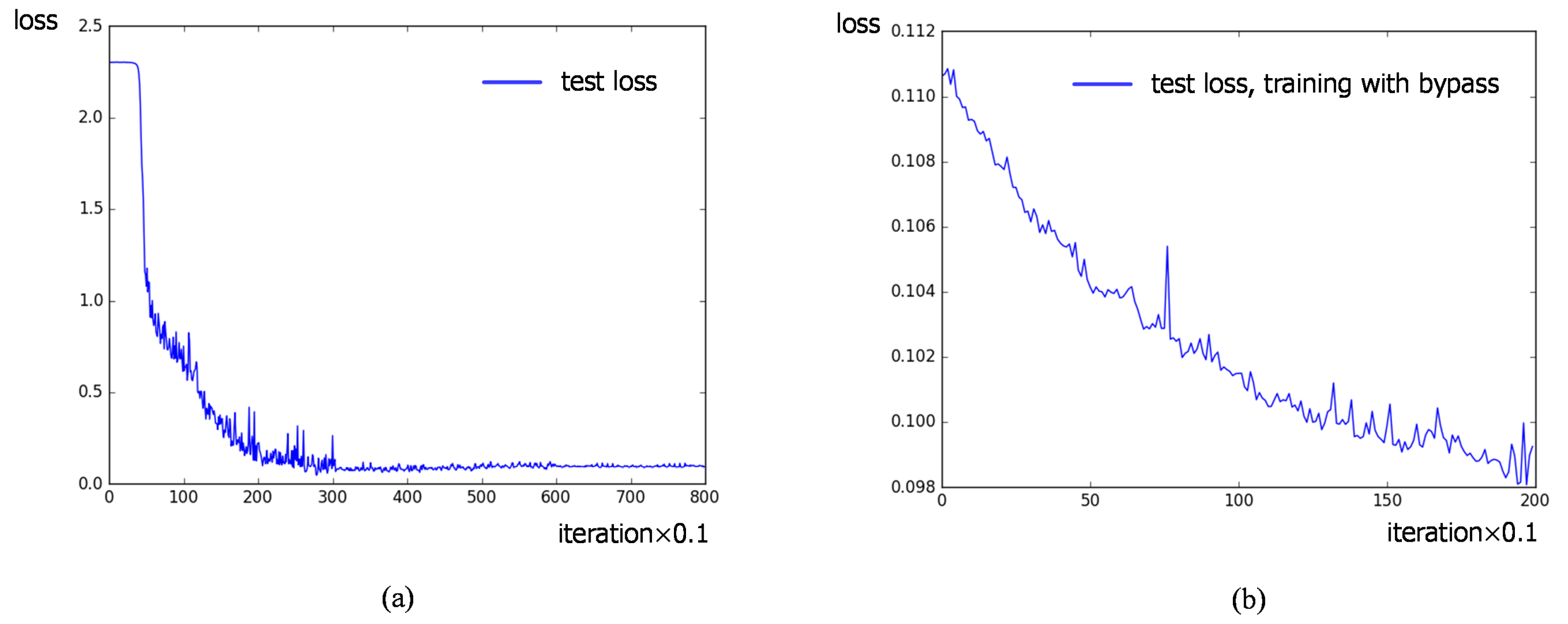
Figure 12.
Recognition rate of different methods with full training sets.
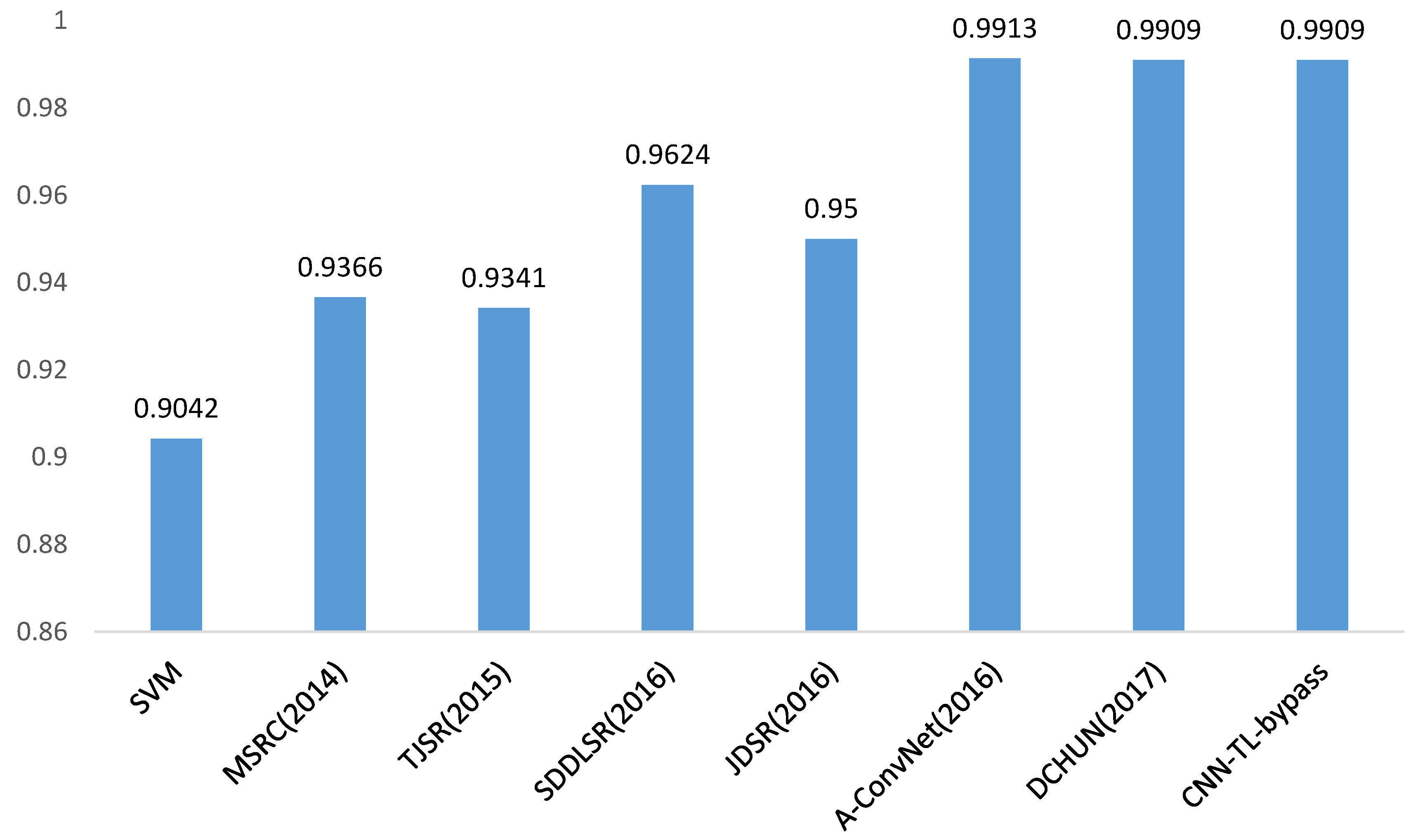
Figure 13.
Recognition rate of different methods with reducing training sets.
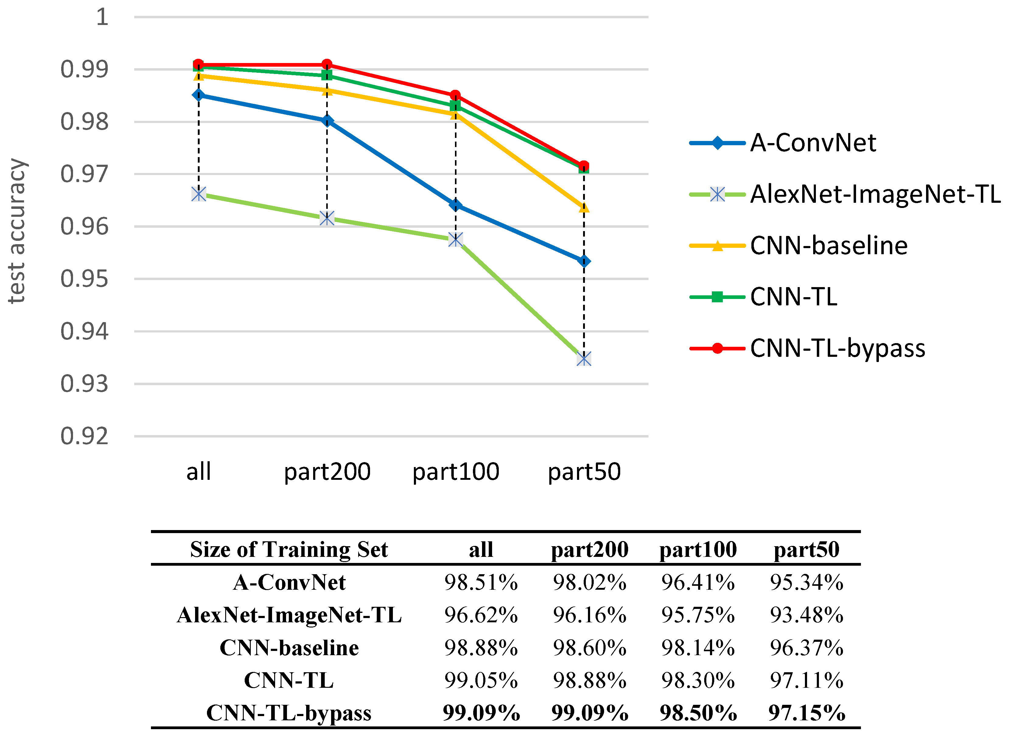
Figure 14.
Testing loss curve during training. (a,b) the testing curve of baseline and transfer learning with 200 training images per category; (c,d) the testing curve of baseline and transfer learning with 50 training images per category.
Figure 14.
Testing loss curve during training. (a,b) the testing curve of baseline and transfer learning with 200 training images per category; (c,d) the testing curve of baseline and transfer learning with 50 training images per category.


Table 1.
Design scheme of classification pathway.
| Layer | Kernel Size | Channel | Padding |
|---|---|---|---|
| conv1 | 5 × 5 | 48 | 2 |
| conv2 | 5 × 5 | 96 | 2 |
| conv3 | 3 × 3 | 128 | 1 |
| conv4 | 3 × 3 | 128 | 1 |
| conv5 | 3 × 3 | 256 | 1 |
| Number of Neurons | |||
| fc6 | 128 (optional) | ||
| fc7 | 10 | ||
Table 2.
Training and testing dataset.
| Category | 2S1 | BMP2 | BRDM2 | BTR60 | BTR70 | D7 | T62 | T72 | ZIL131 | ZSU23 | Total |
|---|---|---|---|---|---|---|---|---|---|---|---|
| Training() | 299 | 233 | 298 | 256 | 233 | 299 | 299 | 232 | 299 | 299 | 2747 |
| Testing() | 274 | 195 | 274 | 295 | 196 | 274 | 273 | 196 | 274 | 274 | 2425 |
Table 3.
Classification pathway parameter initialization (Gaussian distribution).
| Layer | Conv1 | Conv2 | Conv3 | Conv4 | Conv5 | Fc6 | Softmax |
|---|---|---|---|---|---|---|---|
| weight (std) | 0.04 | 0.02 | 0.04 | 0.04 | 0.03 | 0.002 | 0.04 |
Table 4.
Confusion matrix of 10-class recognition result (baseline).
| Category | 2S1 | BMP2 | BRDM2 | BTR60 | BTR70 | D7 | T62 | T72 | ZIL131 | ZSU234 | Accuracy |
|---|---|---|---|---|---|---|---|---|---|---|---|
| 2S1 | 270 | 0 | 0 | 0 | 0 | 0 | 3 | 0 | 0 | 1 | 98.54% |
| BMP2 | 0 | 180 | 0 | 0 | 0 | 0 | 0 | 15 | 0 | 0 | 92.3% |
| BRDM2 | 0 | 3 | 270 | 0 | 0 | 0 | 0 | 1 | 0 | 0 | 98.54% |
| BTR60 | 0 | 1 | 0 | 195 | 0 | 0 | 0 | 0 | 0 | 0 | 99.49% |
| BTR70 | 1 | 0 | 1 | 0 | 182 | 0 | 2 | 9 | 0 | 0 | 93.33% |
| D7 | 0 | 0 | 0 | 0 | 0 | 272 | 0 | 0 | 0 | 0 | 100% |
| T62 | 0 | 0 | 0 | 0 | 0 | 1 | 272 | 0 | 0 | 0 | 99.63% |
| T72 | 0 | 0 | 0 | 0 | 0 | 0 | 1 | 195 | 0 | 0 | 99.49% |
| ZIL131 | 0 | 0 | 0 | 0 | 0 | 0 | 0 | 0 | 274 | 0 | 100% |
| ZSU234 | 0 | 0 | 0 | 0 | 0 | 0 | 0 | 0 | 0 | 274 | 100% |
| Accuracy | 98.3% | ||||||||||
Table 5.
Reconstruction loss of each layer (baseline).
| Training Layer | Conv1 | Conv2 | Conv3 | conv4 | conv5 |
|---|---|---|---|---|---|
| loss | 0.1977 | 0.336 | 0.43 | 0.45 | 0.5 |
Table 6.
Average kernel variation(%) in L2-norm.
| Layer (Kernels Num.) | Conv1(48) | Conv2(96) | Conv3(128) | Conv4(128) | Conv5(256) |
|---|---|---|---|---|---|
| Changes(%) in L2-norm | 0.36 | 0.07 | 0.1 | 0.1 | 0.1 |
Table 7.
Confusion matrix of 10-class recognition results (transfer learning).
| Category | 2S1 | BMP2 | BRDM2 | BTR60 | BTR70 | D7 | T62 | T72 | ZIL131 | ZSU234 | Accuracy |
|---|---|---|---|---|---|---|---|---|---|---|---|
| 2S1 | 274 | 0 | 0 | 0 | 0 | 0 | 0 | 0 | 0 | 0 | 100% |
| BMP2 | 0 | 194 | 1 | 0 | 0 | 0 | 0 | 0 | 0 | 0 | 99.49% |
| BRDM2 | 1 | 2 | 271 | 0 | 0 | 0 | 0 | 0 | 0 | 0 | 98.9% |
| BTR60 | 0 | 0 | 0 | 196 | 0 | 0 | 0 | 0 | 0 | 0 | 100% |
| BTR70 | 1 | 1 | 0 | 5 | 182 | 0 | 4 | 1 | 1 | 0 | 93.3% |
| D7 | 0 | 0 | 0 | 0 | 0 | 271 | 1 | 0 | 2 | 0 | 98.9% |
| T62 | 0 | 0 | 0 | 0 | 0 | 1 | 272 | 0 | 0 | 0 | 99.63% |
| T72 | 0 | 1 | 0 | 0 | 1 | 0 | 0 | 194 | 0 | 0 | 98.9% |
| ZIL131 | 0 | 0 | 0 | 0 | 0 | 0 | 0 | 0 | 274 | 0 | 100% |
| ZSU234 | 0 | 0 | 0 | 0 | 0 | 0 | 0 | 0 | 0 | 274 | 100% |
| Accuracy | 99.05% | ||||||||||
Table 8.
Kernel variations in L2-norm of each convolutional layer (primary target task).
| Layer | Conv1 | Conv2 | Conv3 | Conv4 | Conv5 |
|---|---|---|---|---|---|
| Numbers of Kernels (Changes > 30%) | 37/48 | 5/96 | 0/128 | 0/128 | 7/256 |
Table 9.
Confusion matrix of 10-class recognition result (AlexNet-ImageNet-TL).
| Category | 2S1 | BMP2 | BRDM2 | BTR60 | BTR70 | D7 | T62 | T72 | ZIL131 | ZSU234 | Accuracy |
|---|---|---|---|---|---|---|---|---|---|---|---|
| 2S1 | 272 | 0 | 0 | 0 | 0 | 0 | 1 | 0 | 0 | 1 | 99.27% |
| BMP2 | 3 | 171 | 0 | 3 | 7 | 0 | 0 | 1 | 1 | 0 | 91.93% |
| BRDM2 | 0 | 2 | 264 | 3 | 2 | 0 | 0 | 3 | 0 | 0 | 96.35% |
| BTR60 | 3 | 1 | 1 | 189 | 1 | 0 | 0 | 1 | 0 | 0 | 96.43% |
| BTR70 | 0 | 1 | 0 | 6 | 177 | 0 | 4 | 6 | 0 | 1 | 90.77% |
| D7 | 0 | 0 | 0 | 0 | 0 | 266 | 8 | 0 | 0 | 0 | 97.08% |
| T62 | 0 | 0 | 0 | 0 | 0 | 2 | 270 | 0 | 1 | 0 | 98.9% |
| T72 | 0 | 1 | 1 | 3 | 2 | 0 | 2 | 186 | 0 | 1 | 94.9% |
| ZIL131 | 0 | 0 | 0 | 0 | 0 | 0 | 0 | 0 | 274 | 0 | 100% |
| ZSU234 | 0 | 0 | 0 | 0 | 0 | 0 | 0 | 0 | 0 | 274 | 100% |
| Accuracy | 96.62% | ||||||||||
© 2017 by the authors. Licensee MDPI, Basel, Switzerland. This article is an open access article distributed under the terms and conditions of the Creative Commons Attribution (CC BY) license (http://creativecommons.org/licenses/by/4.0/).
Share and Cite
MDPI and ACS Style
Huang, Z.; Pan, Z.; Lei, B. Transfer Learning with Deep Convolutional Neural Network for SAR Target Classification with Limited Labeled Data. Remote Sens. 2017, 9, 907. https://doi.org/10.3390/rs9090907
AMA Style
Huang Z, Pan Z, Lei B. Transfer Learning with Deep Convolutional Neural Network for SAR Target Classification with Limited Labeled Data. Remote Sensing. 2017; 9(9):907. https://doi.org/10.3390/rs9090907
Chicago/Turabian StyleHuang, Zhongling, Zongxu Pan, and Bin Lei. 2017. "Transfer Learning with Deep Convolutional Neural Network for SAR Target Classification with Limited Labeled Data" Remote Sensing 9, no. 9: 907. https://doi.org/10.3390/rs9090907
Note that from the first issue of 2016, this journal uses article numbers instead of page numbers. See further details here.