Improving Satellite-Driven PM2.5 Models with VIIRS Nighttime Light Data in the Beijing–Tianjin–Hebei Region, China


Institute of Urban Meteorology, China Meteorological Administration, Beijing 100089, China
*
Author to whom correspondence should be addressed.
Remote Sens. 2017, 9(9), 908; https://doi.org/10.3390/rs9090908
Submission received: 11 August 2017
/
Revised: 28 August 2017
/
Accepted: 30 August 2017
/
Published: 31 August 2017
Abstract
:Previous studies have estimated ground-level concentrations of particulate matter 2.5 (PM2.5) using satellite-derived aerosol optical depth (AOD) in conjunction with meteorological and land use variables. However, the impacts of urbanization on air pollution for predicting PM2.5 are seldom considered. Nighttime light (NTL) data, acquired with the Visible Infrared Imaging Radiometer Suite (VIIRS) aboard the Suomi National Polar-orbiting Partnership (S-NPP) satellite, could be useful for predictions because they have been shown to be good indicators of the urbanization and human activity that can affect PM2.5 concentrations. This study investigated the potential of incorporating VIIRS NTL data in statistical models for PM2.5 concentration predictions. We developed a mixed-effects model to derive daily estimations of surface PM2.5 levels in the Beijing–Tianjin–Hebei region using 3 km resolution satellite AOD and VIIRS NTL data. The results showed the addition of NTL information could improve the performance of the PM2.5 prediction model. The NTL data revealed additional details for predication results in areas with low PM2.5 concentrations and greater apparent seasonal variation due to the seasonal variability of human activity. Comparison showed prediction accuracy was improved more substantially for the model using NTL directly than for the model using the vegetation-adjusted NTL urban index that included NTL. Our findings indicate that VIIRS NTL data have potential for predicting PM2.5 and that they could constitute a useful supplemental data source for estimating ground-level PM2.5 distributions.
1. Introduction
In recent decades, rapid economic development in China has caused severe environmental pollution, particularly air pollution [1]. As a major air pollutant in many regions of China, fine particulate matter (aerodynamic diameter < 2.5 μm; PM2.5) is associated with various adverse health outcomes including cardiovascular and respiratory diseases [2,3] and consequently, it has received considerable attention [4]. Accurate assessment of air pollution levels and efficacious solutions to public health concerns require measurement of PM2.5 concentrations at high temporal and spatial resolutions [5,6].
Measurements of PM2.5 concentrations can be acquired by ground-based monitoring networks and satellite remote sensing. Although PM2.5 measurements obtained from ground-based monitoring sites are accurate, such networks are typically sparse, which means the spatial coverage of routine measurements is limited [5,7,8]. Because of the large spatial coverage and reliability of repeated measurements, satellite remote sensing provides a potentially cost-effective method for predicting PM2.5 concentrations where ground-monitoring stations are unavailable or sparsely distributed [7,9,10]. Satellite-derived aerosol optical depth (AOD), which reflects the integrated quantity of particles in the vertical atmospheric column [11], has been shown useful for predicting PM2.5 concentrations [10]. Examples of satellite-derived AOD products include the Terra Moderate Resolution Imaging Spectroradiometer (MODIS) data [10,12], Multiangle Imaging Spectroradiometer (MISR) [7,13], and Geostationary Operational Environmental Satellite Aerosol/Smoke Product [14,15]. In early 2014, the MODIS team released the Collection 6 AOD products with reasonably high (3 km) spatial resolution to provide sufficient data for resolving local-scale aerosol features for air quality applications [16]. The new aerosol product presents expected characteristics such as aerosol plumes but it also reveals details of small-scale AOD gradients [16]. Thus, the MODIS 3 km AOD products make it possible to further reduce PM2.5 exposure errors and they have been used successfully for estimating PM2.5 exposure at both regional and national scales [12,17].
Various statistical models have been proposed to establish quantitative relationships between PM2.5 and AOD (e.g., generalized linear regression, generalized additive models, geographically weighted regression, and liner mixed-effects model) [4,5,10,13,15,17]. In addition to AOD values, several studies have also included local meteorological and land use information. Liu et al. incorporated surface temperature, surface wind speed, and mixing height in a predictive model and they further pointed out that road length and population density within areas are effective predictors of PM2.5 [13,15]. Furthermore, a number of useful auxiliary variables such as elevation, source area of PM2.5 emissions, forest cover, and fire count have also been introduced [5,18,19]. As reported in previous studies, these parameters influence the relationship between AOD and ground-level PM2.5 concentrations, and they can be used as additional predictors with which to improve model performance [15,18].
The impact of urbanization on air pollution in predictions of ground-level PM2.5 concentrations at the urban scale has received less attention than it deserves. Few studies have incorporated information concerning urbanization and human activity into PM2.5 prediction models [4,20]. Previous research has demonstrated that population, economic growth, and urban expansion are the three main driving forces that impact PM2.5 concentrations [21,22]. Thus, urbanization indicators (e.g., population, economics, and built-up areas) could potentially be useful predictors of PM2.5 concentrations. However, it is difficult to obtain an urbanization indictor that includes comprehensive information regarding urbanization and human activity to help in the prediction of PM2.5 concentrations. In addition, urbanization data used in existing prediction models cannot satisfy the temporal requirements for estimations of PM2.5 concentrations because there is a lack of long-term urbanization data. For example, Ma et al. used urban cover data from the Global Land Cover Map 2009 (GlobCover2009) to estimate PM2.5 concentrations during 2010–2014 [20]. However, there have been great changes for land cover from 2009 to 2014. Thus, it is difficult to estimate accurate long-term trends in PM2.5 concentrations.
Surface artificial lighting at night has the unique property of reflecting the extent of human activity. Thus, nighttime light (NTL) data provided by both the Defense Meteorological Satellite Program (DMSP) Operational Linescan System (OLS) and the Visible Infrared Imaging Radiometer Suite (VIIRS) sensor on the Suomi National Polar-orbiting Partnership (NPP) Satellite, have been used extensively as proxies for the urban geographic footprint of human activities [23,24]. Many previous studies have revealed strong relationships between NTL data and urbanization [25], population [26], energy consumption [27], and gross domestic product [28]. The NTL measured by the Day/Night Band (DNB) on the VIIRS sensor has higher spatial and radiometric resolutions than the DMSP/OLS and it practically eliminates three critical problems that beset the earlier satellite program: saturation, blooming, and a lack of onboard calibration. The VIIRS NTL has been shown to be a good indicator of built-up areas [29], population, and economics [30]; hence, the capability of VIIRS NTL in characterizing urbanization provides an opportunity to help in estimations of PM2.5 concentrations. However, VIIRS NTL has not been used before in statistical models for predicting PM2.5 concentrations.
This study developed a mixed-effects model to estimate ground-level PM2.5 concentrations using the MODIS 3 km resolution AOD products, together with meteorological and VIIRS NLT data. The objectives of this study were to investigate how NTL data could be incorporated into a statistical model for predicting ground-level PM2.5 concentrations, and to assess whether this parameter could improve PM2.5 prediction accuracy significantly. The remainder of this paper is organized as follows. Section 2 describes the study area and the data used. The method to establish the relationship between AOD and PM2.5 concentration using NTL data is presented in Section 3. The results of the performance of the model are given in Section 4, while discussion of the results and the findings is presented in Section 5. Finally, the derived conclusions are stated in Section 6.
2. Study Area and Data
2.1. Study Area
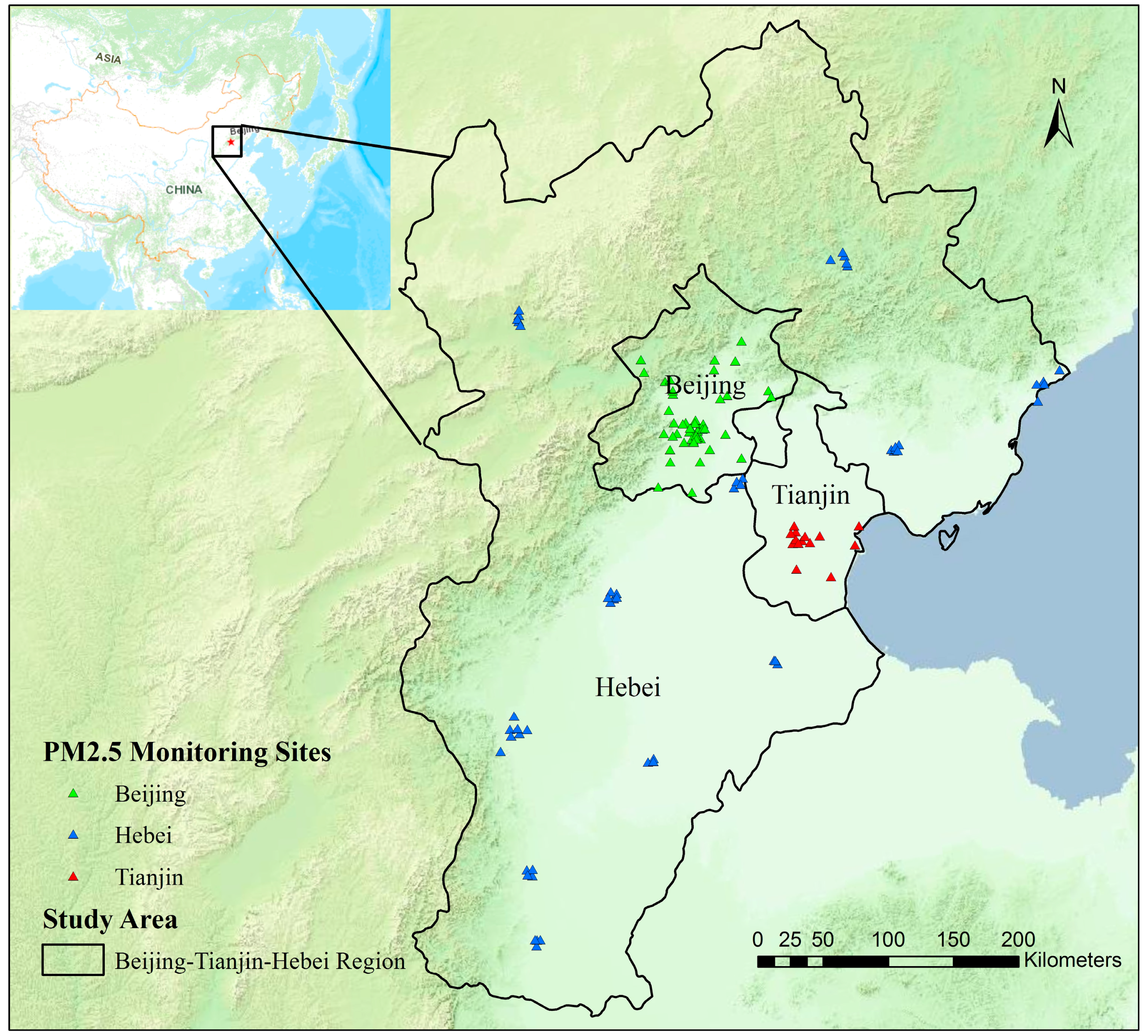
The study area was the Beijing–Tianjin–Hebei (BTH) region, which is situated in northern China (Figure 1). It includes Beijing, Tianjin, and eight neighboring cities in China’s Hebei Province. This area covers the Greater Beijing Economic Hub and its surrounding area, and it is also the core region of the Bohai Bay Trade Hub, having long been the most important political, economic, and cultural center of northern China. Following rapid development, the BTH region is also one of the most polluted city clusters in China [20].
2.2. Ground PM2.5 Measurements
Hourly PM2.5 concentrations, observed at 79 monitoring stations in the BTH region from 2016, were obtained from the website of the China Environmental Monitoring Center (http://106.37.208.233:20035/). We also collected additional data from the website of the Beijing Municipal Environmental Monitoring Center (http://zx.bjmemc.com.cn/). Overall, data from 114 monitoring sites were included in the present study (Figure 1). The ground concentrations measured between 10:00 and 14:00 local time (LT) at each site were averaged to derive daily PM2.5 concentrations that matched the overpass time of the MODIS Terra and Aqua satellites. The study period comprised the entire year of 2016, spanning 366 days.
2.3. Remote Sensing Data
2.3.1. MODIS 3 km AOD Products and Calibration
We obtained MODIS Collection 6 Level 2 aerosol products with 3 km spatial resolution for 2016 from NASA Level 1 and the Atmosphere Archive and Distribution System (accessed at https://ladsweb.nascom.nasa.gov/data/search.html). The retrieval algorithm of the higher resolution AOD product is similar to that of the 10 km AOD product, but it averages 6 × 6 pixels in a single retrieval box rather than 20 × 20 pixels after cloud screening and other surface mask processes [16,31]. The MODIS 3 km AOD products have been validated by ground-based data from six Aerosol Robotic Network (AERONET) sites in China and the spatiotemporal variations of 3 km AOD showed good agreement with the AERONET [32].
In this study, Aqua (overpass at ~13:30 LT) and Terra (overpass at ~10:30 LT) MODIS AOD data at 550 nm were first combined and averaged to improve the spatial coverage. In grid cells that had both Terra and Aqua AODs, the averaged value represented the mean of the AOD distribution from 10:00 to 14:00 LT. However, there were many days when only one of the two retrievals was available. Therefore, when combining the two MODIS products, the averaged AOD of a grid cell was biased toward either the morning or afternoon condition. To overcome this bias, Lee et al. [10] used the average Terra AOD/Aqua AOD ratio to estimate the missing AOD values. In this study, to exploit the measurements of both satellites fully, we fitted a simple linear regression to define the relationship between the daily mean AOD values of Terra and Aqua [6]. The relationship between the Aqua and Terra AODs for different seasons was found similar and therefore, we built the regression model using annual data. The derived regression equation was as follows:
where is the AOD. A value of R2 = 0.77 was obtained for both regression models. The missing AOD value was estimated using the above regression equation and then averaged. Consequently, each AOD grid cell contained a mean value that better represented the average conditions from 10:00 to 14:00 LT.
2.3.2. NDVI Data
We considered the Normalized Difference Vegetation Index (NDVI) in the model development process because a previous study has reported that forest cover can affect the AOD–PM2.5 relationship [5]. The Terra MODIS NDVI data used in this study constituted the MOD13A2 products, which are provided every 16 days at 1 km spatial resolution. MOD13A2 data are computed from atmospherically corrected bidirectional surface reflectance [33]. The 16-day mean values of NDVI were used as covariates in the PM2.5 model.
2.3.3. VIIRS NTL and Urban Index Based on NTL
In this study, we examined the impact of urbanization on the relationship between PM2.5 and AOD; the urbanization indicator was expressed by the VIIRS NTL. The VIIRS DNB monthly composites, as a new generation of NTL image products, have been produced and released by the National Oceanic and Atmospheric Administration’s National Centers for Environmental Information [34,35]. As a low NTL detecting band, the DNB can detect NTL within the radiation range of 3.00 to 0.02 , with a span from 75°N to 65°S, 3000 km swath, and a 12-h revisiting period. The spatial resolution is 15 arcseconds (742 m), with a spectral range of 0.5–0.9 μm [36,37]. Monthly VIIRS NTL values were used in this study.
As the primary purpose of this study was to investigate how/whether NTL data could be used to improve prediction accuracy of PM2.5 concentrations, an urban index using VIIRS NTL was also used in the model to compare model performances with different NTL expressions. We selected the Vegetation-Adjusted NTL Urban Index (VANUI) as another urbanization indicator. Following Zhang et al., the VANUI was calculated in this study based on both the VIIRS NTL data and the NDVI data [38]. The equation used for calculating the VANUI is as follows:
where is the VANUI value for the i-th pixel in the j-th evaluation area, is the NDVI value for the i-th pixel, and is the normalized DN value of NTL for the i-th pixel. is calculated using the following equation:
where is the original DN value of NTL for the i-th pixel in the j-th evaluation area and and are the minimum and maximum values of NTL for the j-th evaluation area in the VIIRS NTL data, respectively.
The composite of the mean annual values of the VIIRS NTL data, NDVI, and VANUI for 2016 are presented in Figure 2. Urban areas and areas with high intensity of human activity have high NTL values, high VANUI values, and low NDVI values.
2.4. Meteorological Data
The meteorological data were obtained from the Goddard Earth Observing System Data Assimilation System Forward Processing (GEOS-5 FP). These data included planetary boundary layer height (PBLH, m), relative humility (RH, %), wind speed (WS, m/s), and surface pressure (PS, hPa). The GEOS-5 FP is the latest version of the GEOS-5 meteorological data, with spatial resolution of 0.25° (latitude) × 0.3125° (longitude) in a nested grid that covers China, which has been available since April 2012 [39]. GEOS-5 FP data from 2016 were used in this study for model development and hourly GEOS-5 FP data from 10:00 to 14:00 LT were averaged as daytime meteorological parameters to match the satellite overpass times.
All data were re-projected using the Albers equal area conic projection and resampled to spatial resolution of 3 km. Then, all the data were clipped following administrative boundary data of the study area. Finally, all variables in 2016 were matched by grid cell and date for model fitting.
3. Method
3.1. Model Development
Previous studies have shown that time-varying parameters such as RH, PM2.5 vertical and diurnal concentration profiles, and PM2.5 optical properties can influence the PM2.5–AOD relationship [10,17]. Therefore, we developed a linear mixed-effects (LME) model [10] to account for daily variations of the AOD–PM2.5 relationship. Considering the regional spatial scale of this study, we hypothesize that these time-varying parameters exhibit little spatial variability and consequently, the PM2.5–AOD relationship has minimal spatial variation on any given day. Daily variations of the relationship between additional variables and PM2.5 were not considered in our model because they led to over-fitting of the models. In addition, whether a predictor should be incorporated needs to be tested in the model. We tested other meteorological parameters (e.g., air temperature) and land use types not included in the final models, and no significant improvement was found in the regression performance.
We first fitted three LME models to compare the performances of models with and without NTL predictors: the LME model only with meteorological data (referred to as the Meteor_LME, Equation (4)), LME model without VIIRS NTL data (referred to as the NDVI_LME, Equation (5)), and LME model with VIIRS NTL data (referred to as the NTL_LME, Equation (6)). In addition, we also fitted the LME model using VANUI (referred to as the VANUI_LME, Equation (7)) instead of NTL and NDVI to establish the form of urbanization indicator using NTL that benefitted model performance the most. These models can be expressed as follows:
where (μg/m3) is the averaged observed PM2.5 concentration at grid cell s on day t; and are the fixed and day-specific random intercepts, respectively, (i = 1, 2……) are the fixed slopes for the predictors, and is the random slope for AOD at each day; refers to the MODIS AOD value (unitless) at grid cell s on day t; (m), (%), (m/s), and (hPa) are the meteorological parameters at grid cell s on day t (definitions in Section 2.4); (unitless) is the normalized value of VIIRS NTL data at grid cell s on day t, (unitless) is the MODIS NDVI value at grid cell s on day t, and (unitless) is the index value obtained by combining the NTL and NDVI values (definitions in Section 2.3.3) at grid cell s on day t. In these statistical models, the AOD fixed effect represents the average effect of AOD on PM2.5 for all studied days. The AOD random effects explain the daily variability in the PM2.5–AOD relationship. These equations were applied to the entire fitting dataset to generate the fixed effects intercept and slopes for all the days and the random effects intercept and slopes for each individual day.
3.2. Model Validation
To validate the performances of the four models, commonly used statistical indicators between fitted values from the models and observations were calculated. We calculated the coefficient of determination (R2) to indicate the degree of agreement of fitting between predicted and observed PM2.5 concentrations. The mean prediction error (MPE) and the root mean square prediction error (RMSE) were adopted to evaluate the prediction accuracy of each of the four models. The MPE and RMSE are defined as
and
where is the predicted PM2.5 concentrations, is the observed values, and n is the total number of observations. The goodness of fit of each model was checked using the Akaike information criterion (AIC) and the Bayes information criterion (BIC) [40]. Smaller values of the AIC and the BIC indicate better fitting of the model to the data.
In addition, a 10-fold cross-validation (CV) method was applied to assess potential model over-fitting [41]. The dataset was first split into 10 folds with approximately 10% of the total data points in each fold. In each round of the CV, one fold was used as the test data, the remaining nine folds were used to fit the model, and predictions were made on the held-out test fold. This process was repeated 10 times until each fold had been tested. Furthermore, the same statistics (e.g., R2, MPE, and RMSE) were calculated for the cross-validation results.
4. Results
4.1. Descriptive Statistics
The descriptive statistics of the dependent and predictor variables used in the model fitting are presented in Table 1. There were 3674 matched data records used for the model fitting. The overall mean PM2.5 concentration is 55.20 μg/m3, which is higher than China’s National Ambient Air Quality Standard (NAAQS) of 35.00 μg/m3 for annual mean PM2.5, and the standard deviation (SD) is 42.07 μg/m3. The mean value of MODIS AOD is 0.71, although some sites have high AOD values of >2.00. The normalized NTL for 2016 has a mean value of 0.22 and the mean NDVI value is 0.42, which means there is relatively high vegetation cover in the BTH region. The RH has a relatively small mean value of 33%, which implies a relatively dry atmospheric environment. The PBLH (1636.88 ± 623.41 m) is more variable in comparison with other meteorological variables.
4.2. Model Fitting and Validation
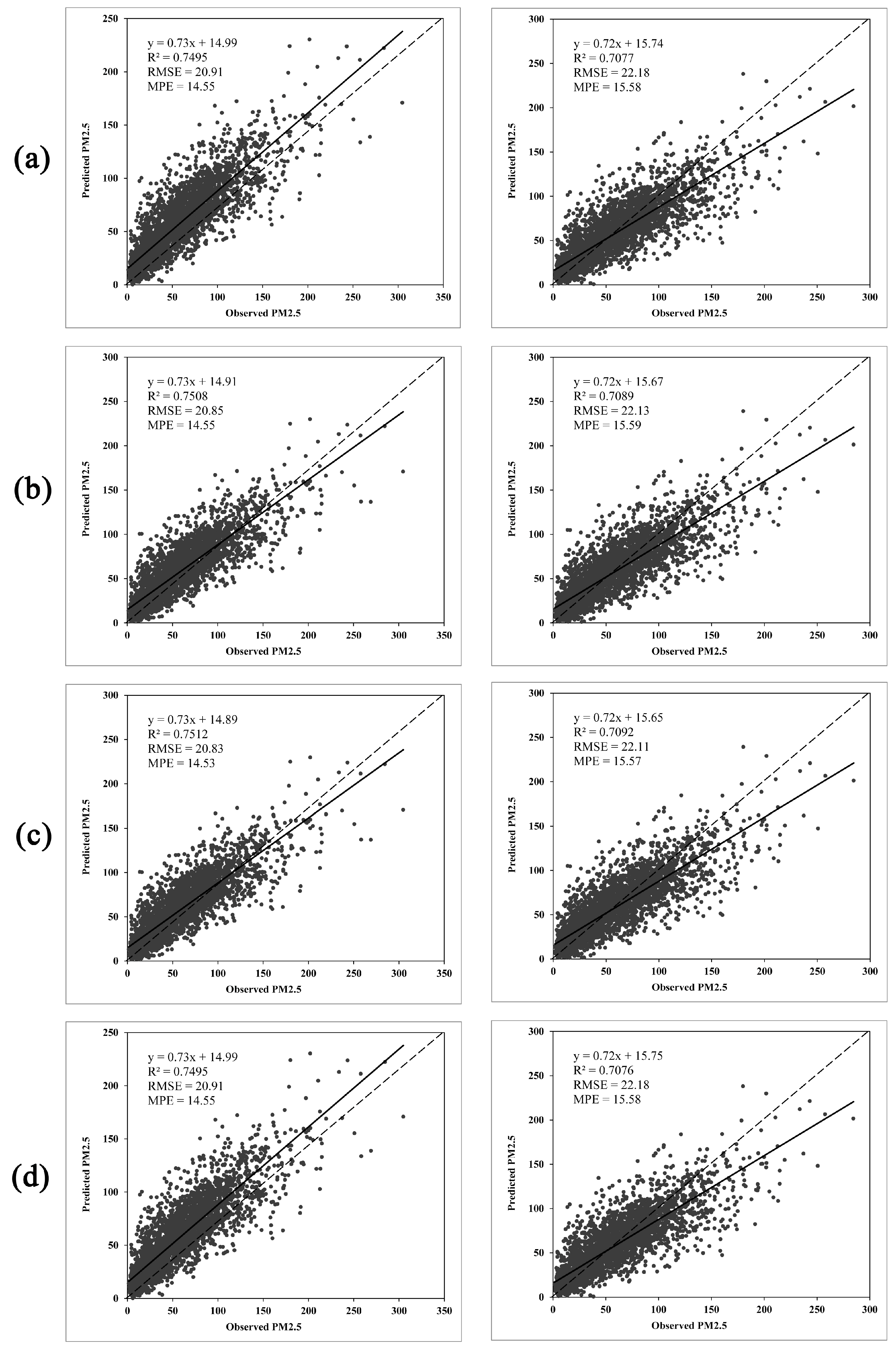
Table 2 summarizes the fixed effect and random estimates of the four LME models with different combinations of predictors. Daily AOD–PM2.5 relationships of 203 days were calculated using the LME models. The fixed terms of the intercept and slopes for the Meteor_LME and VANUI_LME models are different to these for the NDVI_LME and NTL_LME models, while the standard errors (SEs) of the fixed terms for the four models are similar. The SEs of the daily specific intercepts and slopes for the four models are about 23.00 and 26.00, respectively. The fixed effects and random effects results show all four LME models can reflect the temporal variations of AOD–PM2.5 relationships, irrespective of whether the predictor variables are different. Table 2 also shows that incorporating the VIIRS NTL data into the LME model produced the smallest values of the AIC and the BIC, indicating better model fitting.
Figure 3 shows the model fitting and CV results for the different models. For the four model fittings, the overall values of R2 between the predicted and observed PM2.5 concentrations are all >0.75, with RMSEs of around 20 μg/m3 and MPEs of around 14.5. The CV R2 values of the four models are all >0.70, which reflects a decrease of 0.04 compared with the model fitting results. The CV RMSE values increase by about 1 μg/m3 for the four models, which suggests the models are not substantially over-fitted. Comparison of the CV statistics of the Meteor_LME model and the NDVI_LME model, by adding the NDVI predictor to the model, shows the overall prediction accuracy was improved. The CV RMSPE decreased by 0.06 μg/m3, representing a 0.29% reduction. The NTL_LME fitting and CV R2 values are 0.7512 and 0.7092 (Figure 3c), respectively, which indicate this model performed best of all the models. Comparison of the other three models (Figure 3a,b,d) with the NTL_LME model (Figure 3c) shows the NTL model marginally increased the R2 values. The CV results indicate all models have a trend to overestimate the PM2.5 concentrations in relation to relatively low PM2.5 observations and to underestimate the PM2.5 values in relation to relatively high PM2.5 observations. The Meteor_LME model produced the worst model fitting and it yielded greater bias than the other models.
Both the NTL_LME and VANUI_LME models included NTL data but their results are different. The NTL_LME results improved the performance of the Meteor_LME model, but the VANUI_LME results had little effect on the Meteor_LME model. This result suggests that the form of the urbanization indicator using NTL could affect the results of the models, and that NTL as a predictor variable added to the model directly performed better than using the form of the urban index as a predictor variable.
4.3. Annual and Seasonal Mean PM2.5 Concentrations
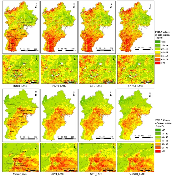
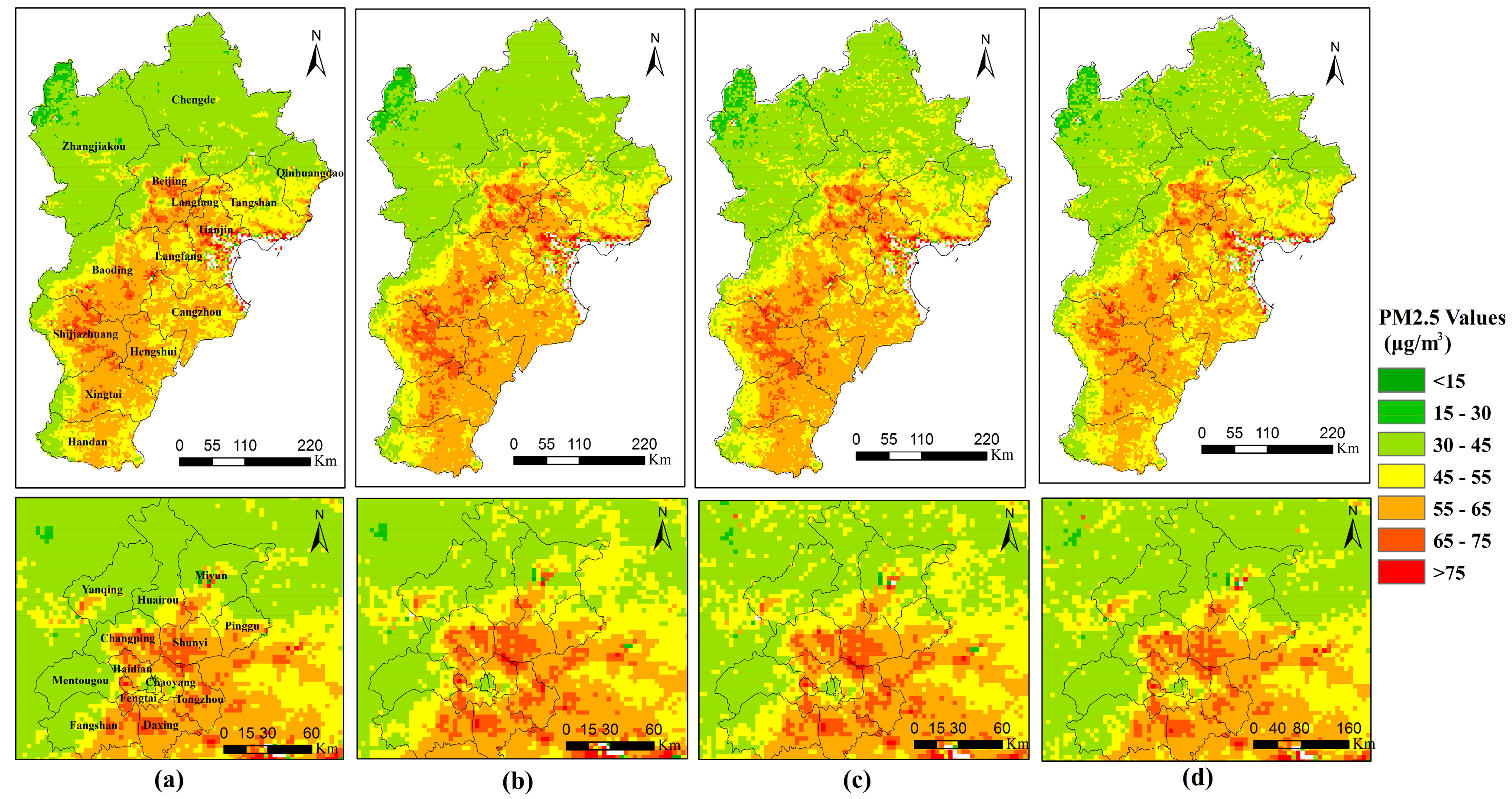
Figure 4 shows the annual mean PM2.5 concentrations predicted by the different models. The results show that the patterns of PM2.5 estimates from the four models are largely similar. Spatially, there is a southeast-to-northwest gradient in the predicted PM2.5 distribution. High concentrations are found in Beijing and the south of Hebei Province, while low concentrations appear in the north of Hebei Province. From the details of Beijing, highly urbanized and populated areas such as Haidian, Shijingshan, and Fengtai exhibit higher PM2.5 levels compared with rural areas such as Huairou. Furthermore, higher PM2.5 levels are predicted over southern regions and lower values predicted over northern and western suburban districts.
Comparison of the PM2.5 concentrations estimated by the different models shows those models using NTL, either integrated as an urban index (VANUI_LME) or directly as a variable (NTL_LME), generated greater detail of the predicted surface than those not using NTL data (i.e., Meteor_LME and NDVI_LME), especially in areas with low PM2.5 values (e.g., Chengde and Zhangjiakou). In this region, PM2.5 estimates generated from the models with NTL were higher than those estimated from the models without NTL. In addition, the NTL_LME and NDVI_LME models provided higher predictions than the Meteor_LME and VANUI_LME models in Shijiazhuang and Baoding.
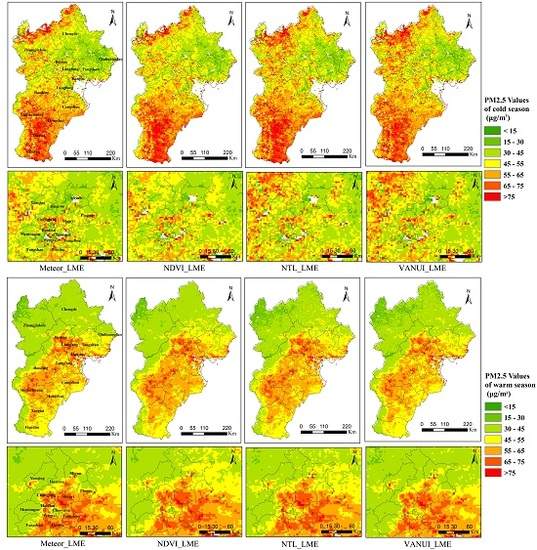
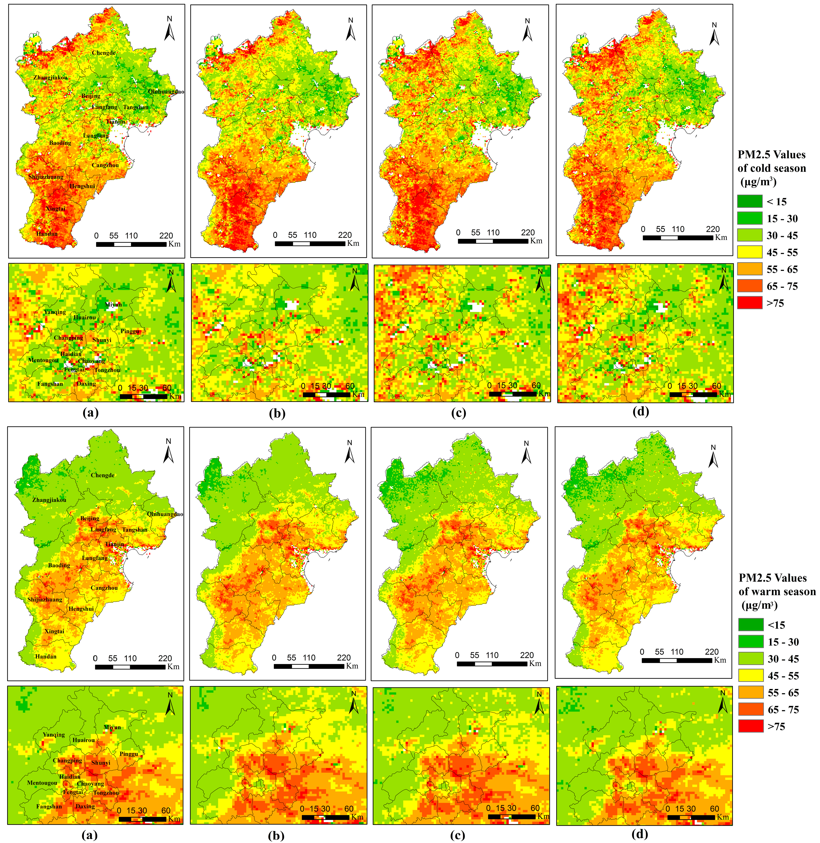
Because of limited satellite data in winter (January, February, and December), the data were grouped into two seasons: warm (15 April–14 October) and cold (15 October–14 April). Figure 5 shows the two seasonal mean distributions of PM2.5 concentration. The PM2.5 pattern of the BTH region exhibits distinct seasonal variational characteristics, with the highest pollution occurring in the cold season and the lowest pollution occurring in the warm season (except for Beijing). The predicted PM2.5 concentrations within the warm season range from 8 to 190 μg/m3, while the predicted PM2.5 concentrations within the cold season range from 2 to 300 μg/m3. Such seasonal variation can be attributed to the mixed contributions from meteorological conditions and local emission sources.
Comparison of Figure 5 shows the mean PM2.5 estimates generated from models with NTL have higher values in the cold season and lower values in the warm season than models without NTL. This indicates that models with NTL exhibit more significant seasonal variation than models without NTL, especially in northern areas of the BTH region. For example, the average PM2.5 concentration within the cold season predicted by the NTL_LME model is 54.65 μg/m3, which is higher than the PM2.5 concentration predicted by the NDVI_LME model (53.09 μg/m3). Conversely, the average PM2.5 concentration within the warm season predicted by the NTL_LME model is 47.95 μg/m3, which is lower than the PM2.5 concentration predicted by the NDVI_LME model (48.44 μg/m3). In addition, the differences between PM2.5 concentrations estimated by models with and without NTL are larger in the cold season than in the warm season. The level of coal and biomass combustion associated with heating increases in winter, which represents human activities. NTL is used as an indicator of urban areas, human activities, and population density. Consequently, the contribution of NTL to predictions of PM2.5 concentrations is correspondingly higher in winter.
5. Discussion
This paper evaluated the performance of VIIRS NTL data when used as a predictor for PM2.5 concentration estimations. In brief, it was proven that VIIRS NTL data have considerable potential to provide additional predictive power for estimations of PM2.5 concentrations.
Our results showed that the incorporation of NTL data as a predictor could improve PM2.5 prediction accuracy, and that NTL data might partially account for PM2.5 variability in the models, which suggests that elevated PM2.5 levels cannot be explained fully by AOD. The experimental results also showed that models with NTL exhibited more significant seasonal variation than models without NTL. Because NTL can reflect human activity, which varies seasonally, the impact of human activity on the AOD–PM2.5 relationship can account for the seasonal variability exhibited by those models with NTL. Furthermore, the differences between the PM2.5 concentrations estimated by models with and without NTL were larger in the cold season than in the warm season. In winter, the main contribution to elevated PM2.5 concentrations is from coal and biomass combustion for heating. This information might be not captured by MODIS AOD, whereas NTL as an indicator of human activity can reflect the effect of heating to some extent. Thus, NTL data might introduce into the models additional PM2.5 emission sources missed by MODIS AOD, which could lead to predictions of PM2.5 that are more accurate. As the impact of human activity on PM2.5 concentrations is more apparent in the cold season than in the warm season, the differences between models with and without NTL are larger in the cold season.
It should be noted that the form in which NTL data are incorporated within the models could affect the applicability of NTL data in air pollution monitoring studies. We compared the performances of models with NTL data and with VANUI, which is an urban index using NTL and NDVI. The model based on NTL and the NDVI variable appeared to provide better estimation performance than the model based solely on VANUI. This might be because the VANUI focuses on inner-urban variations more than on urbanization characteristics [38]. Further research is needed to explore the potential data fusion approaches for better use of NTL data in statistical models for PM2.5 concentration predictions.
It should also be mentioned that NTL data can be acquired easily and are free to download, while it is difficult to obtain other urban indicator data such as accurate spatial distributions of population. In addition, VIIRS can provide data from 2013 to the present, and the DMSP/OLS NTL has a long historical archive. Our statistical model for predicting PM2.5 concentrations could be further used to produce long-term time series of serious PM2.5 exposure, which could then be applied in long-term epidemiological studies. Furthermore, we used high spatial resolution MODIS 3 km AOD data to estimate high spatial resolution daily average PM2.5 concentrations. Higher resolution data could help reveal additional local details of the relationship and thus, the acquisition of such data is desirable.
Although the developed LME models with NTL produced promising results, some limitations remain. We combined Terra MODIS data and Aqua MODIS data to improve the spatial coverage of the MODIS 3 km AOD products, but there were still a number of missing data. Further studies could introduce additional estimators to fill the gaps in areas where AOD is not retrieved. Furthermore, the PM2.5–AOD relationship varies in both space and time, but the LME model used in our study incorporates only the temporal variation in the PM2.5–AOD association. We will develop new statistical models with NTL that can include both the spatial and the temporal variabilities in the PM2.5–AOD relationship.
6. Conclusions
In this paper, we assessed the applicability of VIIRS/DNB NTL data in estimating surface PM2.5 concentrations using an LME model in the BTH region of China in 2016. The results indicated that NTL data were an effective predictor of PM2.5 concentrations. Of the models examined, the model incorporating NTL provided better performance and illustrated more detail in the predicted surface, especially in areas with low PM2.5 values. Our analysis also showed that the introduction of NTL into PM2.5 prediction models increased the seasonal variability. The results of this study provide insight into the possibility of enhancing predictions of surface PM2.5 concentrations by incorporating NTL data. The adoption of our method could help in investigations of the impact of urbanization on PM2.5 concentrations.
Acknowledgments
Supported by the Beijing Natural Science Foundation (8174066) and the Ministry of Science and Technology of China (Grant No. IUMKY201612). We thank James Buxton MSc from Liwen Bianji, Edanz Group China (www.liwenbianji.cn./ac), for editing the English text of this manuscript.
Author Contributions
Xiya Zhang and Haibo Hu conceived and designed the experiments. Xiya Zhang mainly analyzed the data and wrote the paper. Haibo Hu designed and revised the paper.
Conflicts of Interest
The authors declare no conflict of interest.
References
- Xu, P.; Chen, Y.; Ye, X. Haze, air pollution, and health in China. Lancet 2013, 382, 2067. [Google Scholar] [CrossRef]
- Dominici, F.; Peng, R.D.; Bell, M.L.; Pham, L.; McDermott, A.; Zeger, S.L.; Samet, J.M. Fine particulate air pollution and hospital admission for cardiovascular and respiratory diseases. JAMA 2006, 295, 1127–1134. [Google Scholar] [CrossRef] [PubMed]
- Pope, C.A., III; Burnett, R.T.; Thun, M.J.; Calle, E.E.; Krewski, D.; Ito, K.; Thurston, G.D. Lung cancer, cardiopulmonary mortality, and long-term exposure to fine particulate air pollution. JAMA 2002, 287, 1132–1141. [Google Scholar] [CrossRef] [PubMed]
- Ma, Z.; Hu, X.; Huang, L.; Bi, J.; Liu, Y. Estimating ground-level PM2.5 in China using satellite remote sensing. Environ. Sci. Technol. 2014, 48, 7436–7444. [Google Scholar] [CrossRef] [PubMed]
- Hu, X.; Waller, L.A.; Al-Hamdan, M.Z.; Crosson, W.L.; Estes, M.G., Jr.; Estes, S.M.; Quattrochi, D.A.; Sarnat, J.A.; Liu, Y. Estimating ground-level PM2.5 concentrations in the southeastern U.S. Using geographically weighted regression. Environ. Res. 2013, 121, 1–10. [Google Scholar] [CrossRef] [PubMed]
- Hu, X.; Waller, L.A.; Lyapustin, A.; Wang, Y.; Al-Hamdan, M.Z.; Crosson, W.L.; Estes, M.G., Jr.; Estes, S.M.; Quattrochi, D.A.; Puttaswamy, S.J.; et al. Estimating ground-level PM2.5 concentrations in the southeastern United States using MAIAC AOD retrievals and a two-stage model. Remote Sens. Environ. 2014, 140, 220–232. [Google Scholar] [CrossRef]
- Van Donkelaar, A.; Martin, R.V.; Brauer, M.; Kahn, R.; Levy, R.; Verduzco, C.; Villeneuve, P.J. Global estimates of ambient fine particulate matter concentrations from satellite-based aerosol optical depth: Development and application. Environ. Health Perspect. 2010, 118, 847–855. [Google Scholar] [CrossRef] [PubMed]
- Hoff, R.M.; Christopher, S.A. Remote sensing of particulate pollution from space: Have we reached the promised land? J. Air Waste Manag. Assoc. 2009, 59, 645–675. [Google Scholar] [PubMed]
- Engel-Cox, J.A.; Holloman, C.H.; Coutant, B.W.; Hoff, R.M. Qualitative and quantitative evaluation of MODIS satellite sensor data for regional and urban scale air quality. Atmos. Environ. 2004, 38, 2495–2509. [Google Scholar] [CrossRef]
- Lee, H.J.; Liu, Y.; Coull, B.A.; Schwartz, J.; Koutrakis, P. A novel calibration approach of MODIS AOD data to predict PM2.5 concentrations. Atmos. Chem. Phys. 2011, 11, 7991–8002. [Google Scholar] [CrossRef]
- Kahn, R.; Banerjee, P.; McDonald, D.; Diner, D.J. Sensitivity of multiangle imaging to aerosol optical depth and to pure-particle size distribution and composition over ocean. J. Geophys. Res. Atmos. 1998, 103, 32195–32213. [Google Scholar] [CrossRef]
- You, W.; Zang, Z.; Zhang, L.; Li, Y.; Pan, X.; Wang, W. National-scale estimates of ground-level PM2.5 concentration in China using geographically weighted regression based on 3 km resolution MODIS AOD. Remote Sens. 2016, 8, 184. [Google Scholar] [CrossRef]
- Liu, Y.; Franklin, M.; Kahn, R.; Koutrakis, P. Using aerosol optical thickness to predict ground-level PM2.5 concentrations in the St. Louis area: A comparison between MISR and MODIS. Remote Sens. Environ. 2007, 107, 33–44. [Google Scholar] [CrossRef]
- Paciorek, C.J.; Liu, Y.; Moreno-Macias, H.; Kondragunta, S. Spatiotemporal associations between GOES aerosol optical depth retrievals and ground-level PM2.5. Environ. Sci. Technol. 2008, 42, 5800–5806. [Google Scholar] [CrossRef] [PubMed]
- Liu, Y.; Paciorek, C.J.; Koutrakis, P. Estimating regional spatial and temporal variability of PM2.5 concentrations using satellite data, meteorology, and land use information. Environ. Health Perspect. 2009, 117, 886–892. [Google Scholar] [CrossRef] [PubMed] [Green Version]
- Remer, L.A.; Mattoo, S.; Levy, R.C.; Munchak, L.A. MODIS 3 km aerosol product: Algorithm and global perspective. Atmos. Meas. Tech. 2013, 6, 1829–1844. [Google Scholar] [CrossRef]
- Xie, Y.; Wang, Y.; Zhang, K.; Dong, W.; Lv, B.; Bai, Y. Daily estimation of ground-level PM2.5 concentrations over Beijing using 3 km resolution MODIS AOD. Environ. Sci. Technol. 2015, 49, 12280–12288. [Google Scholar] [CrossRef] [PubMed]
- Hu, X.; Waller, L.A.; Lyapustin, A.; Wang, Y.; Liu, Y. Improving satellite-driven PM2.5 models with Moderate Resolution Imaging Spectroradiometer fire counts in the southeastern U.S. J. Geophys. Res. Atmos. 2014, 119, 11375–11386. [Google Scholar] [CrossRef]
- Kloog, I.; Koutrakis, P.; Coull, B.A.; Lee, H.J.; Schwartz, J. Assessing temporally and spatially resolved PM2.5 exposures for epidemiological studies using satellite aerosol optical depth measurements. Atmos. Environ. 2011, 45, 6267–6275. [Google Scholar] [CrossRef]
- Ma, Z.; Hu, X.; Sayer, A.M.; Levy, R.; Zhang, Q.; Xue, Y.; Tong, S.; Bi, J.; Huang, L.; Liu, Y. Satellite-based spatiotemporal trends in PM2.5 concentrations: China, 2004–2013. Environ. Health Perspect. 2016, 124, 184–192. [Google Scholar] [CrossRef] [PubMed]
- Han, L.; Zhou, W.; Li, W.; Li, L. Impact of urbanization level on urban air quality: A case of fine particles (PM(2.5)) in Chinese cities. Environ. Pollut. 2014, 194, 163–170. [Google Scholar] [CrossRef] [PubMed]
- Lin, G.; Fu, J.; Jiang, D.; Hu, W.; Dong, D.; Huang, Y.; Zhao, M. Spatio-temporal variation of PM2.5 concentrations and their relationship with geographic and socioeconomic factors in China. Int. J. Environ. Res. Public Health 2014, 11, 173–186. [Google Scholar] [CrossRef] [PubMed]
- L.Imhoff, M.; Lawrence, W.T.; Stutzer, D.C.; Elvidge, C.D. A technique for using composite DMSP/OLS ‘city lights’ satellite data to accurately map urban areas. Remote Sens. Environ. 1997, 61, 361–370. [Google Scholar] [CrossRef]
- Elvidge, C.D.; Cinzano, P.; Pettit, D.R.; Arvesen, J.; Sutton, P.; Small, C.; Nemani, R.; Longcore, T.; Rich, C.; Safran, J.; et al. The Nightsat mission concept. Int. J. Remote Sens. 2007, 28, 2645–2670. [Google Scholar] [CrossRef]
- Ma, T.; Zhou, C.; Pei, T.; Haynie, S.; Fan, J. Quantitative estimation of urbanization dynamics using time series of DMSP/OLS nighttime light data: A comparative case study from China’s cities. Remote Sens. Environ. 2012, 124, 99–107. [Google Scholar] [CrossRef]
- Sutton, P.; Roberts, D.; Elvidge, C.; Baugh, K. Census from heaven: An estimate of the global human population using night-time satellite imagery. Int. J. Remote Sens. 2001, 22, 3061–3076. [Google Scholar] [CrossRef]
- Elvidge, C.D.; Baugh, K.E.; Dietz, J.B.; Bland, T.; Sutton, P.C.; Kroehl, H.W. Radiance calibration of DMSP/OLS low-light imaging data of human settlements. Remote Sens. Environ. 1999, 68, 77–88. [Google Scholar] [CrossRef]
- Jing, X.; Shao, X.; Cao, C.; Fu, X.; Yan, L. Comparison between the Suomi-NPP day-night band and DSMP/OLS for correlating socio-economic variables at the provincial level in China. Remote Sens. 2016, 8, 17. [Google Scholar] [CrossRef]
- Sharma, R.C.; Tateishi, R.; Hara, K.; Gharechelou, S.; Iizuka, K. Global mapping of urban built-up areas of year 2014 by combining MODIS multispectral data with VIIRS nighttime light data. Int. J. Digit. Earth 2016, 9, 1004–1020. [Google Scholar] [CrossRef]
- Chen, X.; Nordhaus, W. A test of the new VIIRS lights data set: Population and economic output in Africa. Remote Sens. 2015, 7, 4937–4947. [Google Scholar] [CrossRef]
- Hsu, N.C.; Jeong, M.J.; Bettenhausen, C.; Sayer, A.M.; Hansell, R.; Seftor, C.S.; Huang, J.; Tsay, S.C. Enhanced deep blue aerosol retrieval algorithm: The second generation. J. Geophys. Res. Atmos. 2013, 118, 9296–9315. [Google Scholar] [CrossRef]
- He, Q.; Zhang, M.; Huang, B. Spatio-temporal variation and impact factors analysis of satellite-based aerosol optical depth over China from 2002 to 2015. Atmos. Environ. 2016, 129, 79–90. [Google Scholar] [CrossRef]
- Justice, C.O.; Townshend, J.R.G.; Vermote, E.F.; Masuoka, E.; Wolfe, R.E.; Saleous, N.; Roy, D.P.; Morisette, J.T. An overview of MODIS land data processing and product status. Remote Sens. Environ. 2002, 83, 3–15. [Google Scholar] [CrossRef]
- Shi, K.; Yu, B.; Huang, Y.; Hu, Y.; Yin, B.; Chen, Z.; Chen, L.; Wu, J. Evaluating the ability of NPP-VIIRS nighttime light data to estimate the gross domestic product and the electric power consumption of China at multiple scales: A comparison with DMSP-OLS data. Remote Sens. 2014, 6, 1705–1724. [Google Scholar] [CrossRef]
- Mills, S.; Weiss, S.; Liang, C. VIIRS day/night band (DNB) stray light characterization and correction. Proc. SPIE 2013, 8866. [Google Scholar] [CrossRef]
- Elvidge, C.D.; Baugh, K.E.; Zhizhin, M.; Hsu, F.C. Why VIIRS data are superior to DMSP for mapping nighttime lights. Proc. Asia Pac. Adv. Netw. 2013, 35, 62–69. [Google Scholar] [CrossRef]
- Elvidge, C.D.; Zhizhin, M.; Hsu, F.C.; Baugh, K.E. VIIRS Nightfire: Satellite pyrometry at night. Remote Sens. 2013, 5, 4423–4449. [Google Scholar] [CrossRef]
- Zhang, Q.; Schaaf, C.; Seto, K.C. The vegetation adjusted NTL urban index: A new approach to reduce saturation and increase variation in nighttime luminosity. Remote Sens. Environ. 2013, 129, 32–41. [Google Scholar] [CrossRef]
- Lucchesi, R. File Specification for GEOS-5 FP-IT (Forward Processing for Instrument Teams); NASA Goddard Space Flight Center: Greenbelt, MD, USA, 2013.
- Burnham, K.P.; Anderson, R.A. Multimodel inference: Understanding AIC and BIC in model selection. Sociol. Methods Res. 2004, 33, 261–304. [Google Scholar] [CrossRef]
- Kohavi, R. A study of cross-validation and bootstrap for accuracy estimation and model selection. In Proceedings of the 14th International Joint Conference on Artificial Intelligence, Montreal, QC, Canada, 20–25 August 1995; Morgan Kaufmann Publishers Inc.: San Francisco, CA, USA, 1995; Volume 2, pp. 1137–1143. [Google Scholar]
Figure 1.
Study area and locations of PM2.5 monitoring stations.

Figure 2.
Images of mean annual values of the VIIRS NTL data (a), NDVI (b), and VANUI (c) for the BTH region.
Figure 2.
Images of mean annual values of the VIIRS NTL data (a), NDVI (b), and VANUI (c) for the BTH region.
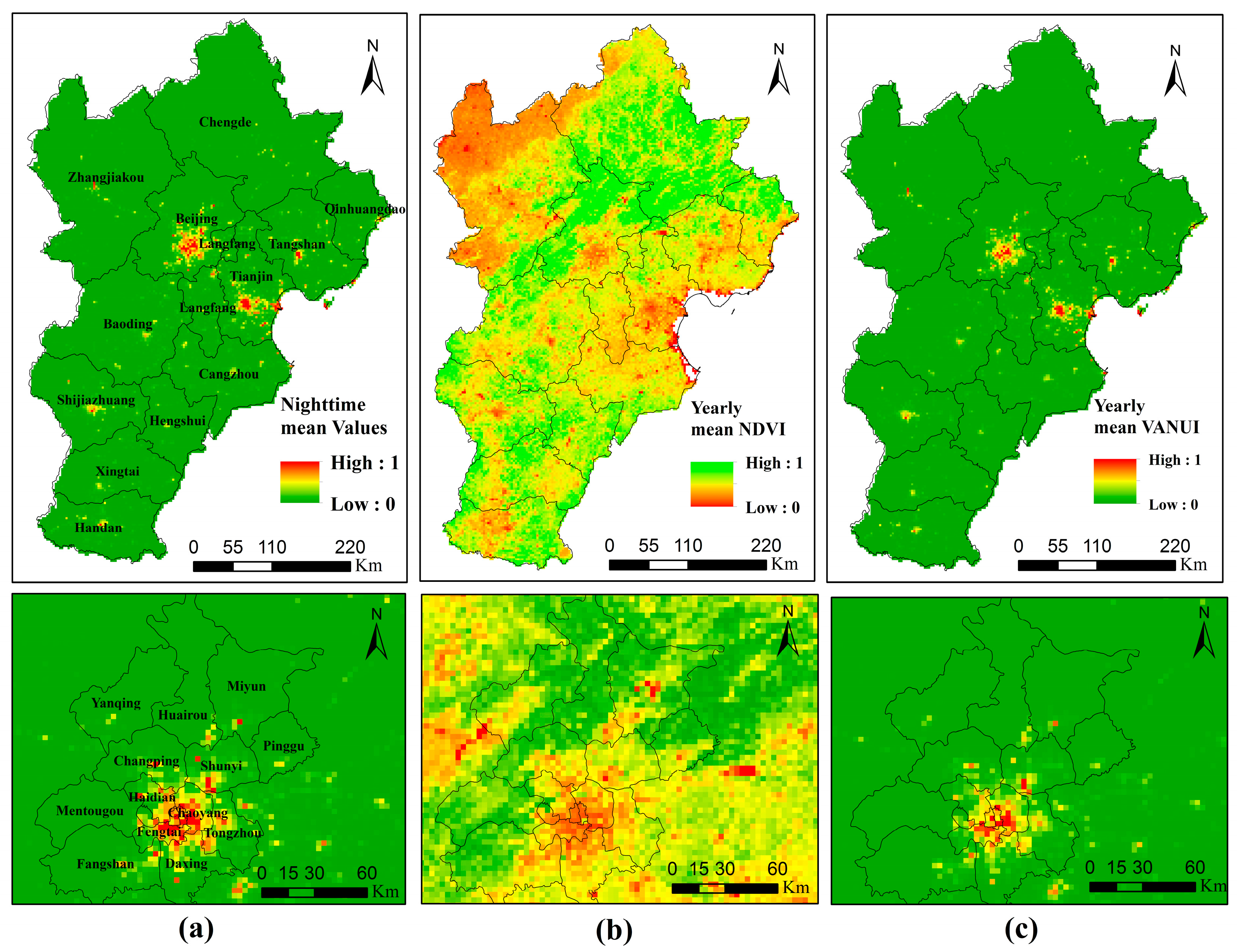
Figure 3.
Results of model fitting (left column) and cross validation (right column). The dashed lines are the 1:1 lines as references: (a) Meteor_LME, (b) NDVI_LME, (c) NTL_LME, and (d) VANUI_LME.
Figure 3.
Results of model fitting (left column) and cross validation (right column). The dashed lines are the 1:1 lines as references: (a) Meteor_LME, (b) NDVI_LME, (c) NTL_LME, and (d) VANUI_LME.

Figure 4.
Annual mean PM2.5 concentration predictions by the different models: (a) Meteor_LME, (b) NDVI_LME, (c) NTL_LME, and (d) VANUI_LME.
Figure 4.
Annual mean PM2.5 concentration predictions by the different models: (a) Meteor_LME, (b) NDVI_LME, (c) NTL_LME, and (d) VANUI_LME.

Figure 5.
Spatial distributions of seasonal mean PM2.5 estimations: cold season (upper) and warm season (lower): (a) Meteor_LME, (b) NDVI_LME, (c) NTL_LME, and (d) VANUI_LME.
Figure 5.
Spatial distributions of seasonal mean PM2.5 estimations: cold season (upper) and warm season (lower): (a) Meteor_LME, (b) NDVI_LME, (c) NTL_LME, and (d) VANUI_LME.


Table 1.
Descriptive statistics summarizing observations for PM2.5 monitoring sites for 2016 (N = 3674).
Table 1.
Descriptive statistics summarizing observations for PM2.5 monitoring sites for 2016 (N = 3674).
| Parameters | Mean | SD | Min | Max |
|---|---|---|---|---|
| PM2.5 (μg/m3) | 55.20 | 42.07 | 1.50 | 304.75 |
| MODIS AOD | 0.71 | 0.48 | 0.03 | 3.75 |
| NTL | 0.22 | 0.17 | 0.00 | 1.00 |
| NDVI | 0.42 | 0.14 | 0.00 | 0.88 |
| VANUI | 0.14 | 0.11 | 0.00 | 0.69 |
| WS (m/s) | 2.90 | 1.56 | 0.14 | 10.76 |
| PS (hPa) | 977.19 | 31.34 | 859.94 | 1032.00 |
| RH (%) | 33 | 14 | 8 | 87 |
| PBLH (m) | 1636.88 | 623.41 | 237.23 | 3704.75 |
Table 2.
Fixed effects and random effects for models and model comparisons.
| Models | Fixed Intercept | SE of Fixed Intercept | Fixed Slopes of AOD | SE of Fixed AOD Slopes | SE of the Random Intercepts | SE of the Random AOD Slopes | AIC | BIC |
|---|---|---|---|---|---|---|---|---|
| Meteor_LME | 24.78 | 14.95 | 27.30 | 2.75 | 23.24 | 26.59 | 33,069.15 | 33,130.95 |
| NDVI_LME | 7.71 | 15.44 | 28.55 | 2.73 | 23.70 | 26.15 | 33,052.28 | 33,125.97 |
| NTL_LME | 8.82 | 15.45 | 28.29 | 2.72 | 23.76 | 26.12 | 33,051.80 | 33,120.26 |
| VANUI_LME | 24.57 | 15.07 | 27.33 | 2.74 | 23.24 | 26.58 | 33,071.13 | 33,139.12 |
© 2017 by the authors. Licensee MDPI, Basel, Switzerland. This article is an open access article distributed under the terms and conditions of the Creative Commons Attribution (CC BY) license (http://creativecommons.org/licenses/by/4.0/).
Share and Cite
MDPI and ACS Style
Zhang, X.; Hu, H. Improving Satellite-Driven PM2.5 Models with VIIRS Nighttime Light Data in the Beijing–Tianjin–Hebei Region, China. Remote Sens. 2017, 9, 908. https://doi.org/10.3390/rs9090908
AMA Style
Zhang X, Hu H. Improving Satellite-Driven PM2.5 Models with VIIRS Nighttime Light Data in the Beijing–Tianjin–Hebei Region, China. Remote Sensing. 2017; 9(9):908. https://doi.org/10.3390/rs9090908
Chicago/Turabian StyleZhang, Xiya, and Haibo Hu. 2017. "Improving Satellite-Driven PM2.5 Models with VIIRS Nighttime Light Data in the Beijing–Tianjin–Hebei Region, China" Remote Sensing 9, no. 9: 908. https://doi.org/10.3390/rs9090908
Note that from the first issue of 2016, this journal uses article numbers instead of page numbers. See further details here.