
Spatial-Spectral-Emissivity Land-Cover Classification Fusing Visible and Thermal Infrared Hyperspectral Imagery


1
The State Key Laboratory of Information Engineering in Surveying, Mapping and Remote Sensing, Wuhan University, Wuhan 430079, China
2
Collaborative Innovation Center of Geospatial Technology, Wuhan University, Wuhan 430079, China
3
College of Computer Science, China University of Geosciences, Wuhan 430074, China
*
Authors to whom correspondence should be addressed.
Remote Sens. 2017, 9(9), 910; https://doi.org/10.3390/rs9090910
Submission received: 16 July 2017
/
Revised: 25 August 2017
/
Accepted: 30 August 2017
/
Published: 5 September 2017
(This article belongs to the Section Remote Sensing Image Processing)
Abstract
:High-resolution visible remote sensing imagery and thermal infrared hyperspectral imagery are potential data sources for land-cover classification. In this paper, in order to make full use of these two types of imagery, a spatial-spectral-emissivity land-cover classification method based on the fusion of visible and thermal infrared hyperspectral imagery is proposed, namely, SSECRF (spatial-spectral-emissivity land-cover classification based on conditional random fields). A spectral-spatial feature set is constructed considering the spectral variability and spatial-contextual information, to extract features from the high-resolution visible image. The emissivity is retrieved from the thermal infrared hyperspectral image by the FLAASH-IR algorithm and firstly introduced in the fusion of the visible and thermal infrared hyperspectral imagery; also, the emissivity is utilized in SSECRF, which contributes to improving the identification of man-made objects, such as roads and roofs. To complete the land-cover classification, the spatial-spectral feature set and emissivity are integrated by constructing the SSECRF energy function, which relates labels to the spatial-spectral-emissivity features, to obtain an improved classification result. The classification map performs a good result in distinguishing some certain classes, such as roads and bare soil. Also, the experimental results show that the proposed SSECRF algorithm efficiently integrates the spatial, spectral, and emissivity information and performs better than the traditional methods using raw radiance from thermal infrared hyperspectral imagery data, with a kappa value of 0.9137.
1. Introduction
Land-cover classification using remote sensing imagery enables us to recognize the physical composition and characteristics of different land-cover types [1,2]. High-resolution visible imagery has been the commonly used data sources for land-cover classification in recent years [3]. The spatial characteristics of visible images reflect the contextual relationships, including the texture features [4], morphological features [5], and object-based features [6], which are important for the classification task. Nowadays, digital cameras are also mounted on the airplane or unmanned aerial vehicle and are used to capture the visible imagery, which can provide detailed shape and texture information with a fine resolution to distinguish the land-cover categories. However, the high spatial resolution imagery acquired in the visible band may be limited at accurately distinguishing the land-cover types with similar spectral values, given that the three bands as R, G and B channels cannot provide enough spectral information. Thermal infrared hyperspectral imagery is a very challenging data source with high potential: it records the emissivity and temperature of the ground objects, regardless of the illumination conditions [7]. The emissivity is closely related to the physical properties of ground surface materials, so thermal infrared hyperspectral imagery is an additional data source for land-cover classification, especially in mineral and urban areas. In addition, the spectral features of minerals in the thermal bands are more salient than those in the visible bands [8], so thermal infrared hyperspectral data can contribute to the urban materials mapping [9]. When conducting land-cover classification fusing visible and thermal infrared hyperspectral imagery, it is intuitive to combine the respective advantages of them efficiently to pursue the better land-cover classification results.
To encourage the fusion of visible and thermal infrared hyperspectral imagery to conduct urban land-cover classification, a dataset was published in the 2014 edition of the IEEE Geoscience and Remote Sensing Data Fusion Contest (DFC), involving coarse-resolution thermal infrared hyperspectral imagery and fine-resolution visible imagery [10]. Based on this DFC dataset, research has been carried out on fusion-based urban classification. Michaelsen [11] utilized self-organizing maps for semi-supervised learning and visualization of the partially labeled data in order to properly fuse the color and texture features from the visible imagery with the thermal spectra from the thermal infrared hyperspectral imagery. Hasani et al. [12] carried out principal component analysis (PCA) transform on the thermal infrared hyperspectral imagery and extracted the gray-level co-occurrence matrix (GLCM), the morphological profile (MP), and the structural feature set (SFS) from the visible data. Finally, they calculated the vegetation index (VI) by calculating the mean value of the thermal infrared hyperspectral imagery bands and the red band of the visible imagery. Li et al. [13] used image gap inpainting to deal with the swath inconsistency between the thermal infrared hyperspectral imagery and visible imagery, and Li also developed a road extraction method through fusing the classification result of the thermal infrared hyperspectral imagery and the segmentation result of the visible imagery to improve the overall classification accuracy. Lu et al. [14] proposed a decision-level-based synergetic classification method to improve the overall classification accuracy of the DFC dataset while minimizing the misclassification of roofs and trees at the same time. In addition, feature extraction is an important process to reduce the dimension of the DFC dataset before classification. Marwaha et al. [15] compared the object-oriented and pixel-based classification approaches on the DFC dataset, and concluded that the object-oriented image analysis technique obtains a high individual user’s accuracy for each classified land-cover class. Akbari et al. [16] used only the thermal infrared hyperspectral imagery of the DFC dataset to map urban land cover. In this method, a support vector machine (SVM) algorithm was first adopted to classify the thermal infrared hyperspectral imagery data, and then a marker-based minimum spanning forest (MMSF) algorithm was applied to increase the accuracy of the less accurately classified land-cover types. Samadzadegan et al. [17] used a semi-supervised local discriminant analysis (SLDA) method to extract features from the thermal infrared hyperspectral imagery data, and extracted spectral and texture features from the visible data. After the spatial-spectral feature space was constructed, a cuckoo search optimization algorithm with mixed binary-continuous coding was adopted for feature selection and SVM parameter determination. To sum up, the existing studies have deemed the thermal infrared hyperspectral data to be a multidimensional data input, and they processed the thermal infrared hyperspectral imagery data of the DFC dataset in the traditional way, where only the raw radiance was considered in the classification task. However, they did not extract the emissivity information from the thermal infrared hyperspectral imagery nor utilize it in the classification task.
In the proposed method, to make full use of the characteristics of the thermal infrared hyperspectral imagery, the emissivity information is used in the classification task. In addition, to take full advantage of the spatial and spectral features of the visible imagery, a conditional random field (CRF) algorithm fusing spatial, spectral, and emissivity information, namely SSECRF, is proposed to integrate the visible imagery and the thermal infrared hyperspectral imagery. In the SSECRF algorithm, the spatial, spectral, and emissivity information is modeled by the potential function. The main contributions of the proposed method are as follows.
- (1)
- Multi-feature fusion framework for high-resolution visible imagery. In the proposed classification framework, features from the high-resolution visible imagery are extracted for different purposes. The spectral feature provides the fundamental information of the ground-object categories, and the visible difference vegetation index (VDVI) [18] is adopted for its effectiveness in green plant separation. In addition, texture features and object-based features are extracted to utilize the spatial correlation between neighboring pixels. A multi-feature fusion framework for the visible data is proposed to integrate the above features to form a spectral-spatial feature set, to realize the feature representation of the high-resolution visible imagery.
- (2)
- Emissivity retrieval from the thermal infrared hyperspectral imagery. The thermal infrared hyperspectral imagery is a potential data source for the identification of man-made objects. In the proposed approach, the emissivity information is retrieved using an automated atmospheric compensation and temperature-emissivity separation (TES) method, called the FLAASH-IR (Fast Line-of-sight Atmospheric Analysis of Spectral Hypercubes—Infrared) algorithm [19], and it is used to construct the spatial-spectral-emissivity feature set. The feature set is then input to the unary potential term in the SSECRF algorithm, leading to a better classification performance.
- (3)
- Spatial-spectral-emissivity land-cover classification based on conditional random fields (SSECRF). The CRF model can incorporate the spatial contextual information in both the labels and observed data. In the proposed SSECRF algorithm, the spatial-spectral feature set from the visible imagery and the emissivity from the thermal infrared hyperspectral imagery are integrated by constructing the energy function to carry out land-cover classification. The spatial-spectral feature and emissivity feature are fused in the unary potential by calculating the probability. The pairwise potential is modeled to consider the spatial correlation of the given imagery, and adjacent pixels can usually be assumed to be the same class. The pairwise potential aims to solve the misclassified categories by utilizing the shape, texture, and spectral features. The spatial, spectral, and emissivity information are fused efficiently in the SSECRF algorithm by the potential terms.
The DFC dataset was adopted to confirm the effectiveness of the proposed SSECRF algorithm, and it was found that the proposed algorithm outperforms the comparative methods in both visual performance and quantitative assessment.
The rest of this paper is organized as follows. Section 2 provides some information related to the experimental datasets. Section 3 introduces some of the basic concepts of emissivity retrieval and CRF, and the proposed algorithm for fusing the visible and thermal infrared hyperspectral imagery data. Meanwhile, we also describe the features extracted from these two types of imagery. In Section 4, we discuss the classification results and parameter sensitivity. Finally, the conclusion is drawn in Section 5.
2. Materials
2.1. Study Site
The study site adopted for this research is located in the Black Lake area of Thetford Mines, province of Québec, Canada (46.047927° N, 71.366893° W), with a variety of natural and man-made objects. Thetford has a temperate marine climate with generally light precipitation throughout the year. The world-famous Thetford mining district (which ceased operations in 2011) lies within an ophiolite complex, an accreted remnant of ancient oceanic crust. Its igneous lithologies have been serpentinised to provide large-scale occurrences of exploitable asbestos minerals. A large amount of chrysotile and white asbestos can be mined from it, for which it has an international reputation. In nearby urban areas, the roads are mainly made of concrete; asphalt shingles are used for the roofs and flat roofs are often covered with an elastomeric membrane. Materials used for roofs, such as garages or sheds, are usually made of sheet metal.
2.2. Dataset Used
The experiments utilized two images with different resolutions covering the same urban area near Thetford Mines in Canada: a coarse-resolution thermal infrared hyperspectral image (Figure 1a) with a 1-m spatial resolution, and a fine-resolution visible image (Figure 1b) at a 0.2-m spatial resolution. The coarse-resolution image was acquired by Hyper-Cam, which is an airborne long wave infrared (LWIR) hyperspectral imagery. The imagery has a spatial dimension of 751 × 874 pixels and has 84 spectral bands between 868 and 1280 cm−1 (7.8 μm and 11.5 μm) at a spectral resolution of 6 cm−1 (full-width half-maximum). The fine-resolution image was acquired using a digital color camera, mounted on the same airborne platform. This image is composed of a series of spatially disjoint sub-images, and red, green, and blue spectral channels, with a spatial size of 3769 × 4386 pixels, which is the uncalibrated digital data. The two sensors were integrated on a gyro-stabilized platform in a fixed-wing aircraft. The images were acquired simultaneously on 21 May 2013, between 22:27:36 and 23:46:01 UTC at a height of 2650 ft (807 m). The training samples with seven land-cover classes are provided using one data subset, as shown in Figure 1c, and the test samples are shown in Figure 1d. Table 1 lists the number of training and test samples for each class.
3. Spatial-Spectral-Emissivity Land-Cover Classification Based on Conditional Random Fields (SSECRF)
3.1. Background
3.1.1. Emissivity Retrieval from the Thermal Infrared Hyperspectral Imagery
Land surface emissivity (LSE), which can be retrieved from the thermal infrared hyperspectral imagery, is an intrinsic property of natural materials, and is sensitive to the material composition, especially to the silicate minerals [20]. The physical background is the fundamental spectral absorption features of silicate minerals and carbonates, which are the major components of the terrestrial surface and the primary constituent of man-made construction objects. The emissivity is critical data for studying soil development and erosion, bedrock mapping, etc. [21], and it is also used to study the relationship between LSE and surface energy budgets [22]. Emissivity data are widely used in mineral mapping [23], gas detection [24], vegetation monitoring [25], etc. With the continuous improvement of sensor manufacturing technology, the acquisition of airborne thermal infrared hyperspectral data has been made possible by the Hyper-Cam and Thermal Airborne Spectrographic Imager (TASI) instruments, which can help us to perform target detection and material classification, regardless of illumination conditions. In the urban land-cover classification task, the thermal infrared hyperspectral imagery is a potential data source for the identification of man-made objects.
3.1.2. Conditional Random Fields (CRF)
CRF is a probabilistic discriminative model, and is the statistical model first used to mark and segment serialized data in 2001 by Lafferty et al. [26]. It directly models the posterior probability of the given observation data so that the contextual information can be considered in both the observed data and the labeled data. As a context classification model, Kumar and Hebert [27] successfully extended this model to two-dimensional image classification and processing in 2003, and the CRF method has also been successfully applied in hyperspectral imagery classification [28,29], man-made scene interpretation [30], building detection from high-resolution interferometric synthetic aperture radar (InSAR) data [31], change detection [32], and high-resolution image classification, integrating the spectral, spatial, and location information by adding the additional higher-order potential in the pairwise CRF model [33].
CRF constructs the conditional probability distribution model of the whole label variables under the condition that the observation variable is given, i.e., to model the maximum a posteriori probability (MAP) distribution directly. In order to build distributions over the combined set of input variables that are always called the observed field, and the output variables that are the label field that we expect to predict, the probabilistic discriminative model can model the posterior probability distribution under the condition of the given observation data as a Gibbs distribution [34] with the following form:
where represents the observed data from the input image, and is the corresponding class labels for the entire image. is the partition function, and is the potential function. Theoretically, the potential function based on the size of the variables in the cliques can be divided into unary potentials, pairwise potentials, and even high-order potentials, and the corresponding Gibbs energy function can be defined as follows:
In the classification of remote sensing imagery, the commonest model is called pairwise CRF, which includes unary and pairwise potentials [35], as shown in the Figure 2 and following formula:
The unary potential is a single point of potential energy which constructs the relationships between observation variables and the corresponding label field. At the same time, pairwise potential , a two-position potential energy, considers the spatial-contextual interaction between the observed variables and the label variables, so it can be regarded as a model that can establish the spatial interaction of the paired random variables in the local neighborhood.
CRF is used to model the posterior probability , as mentioned above. Based on the Bayesian MAP rule, the image classification is designed to find the label image x by maximizing the posterior probability distribution function , and it can be defined as [35]: . Thus, the largest posterior category marker of the CRF can be expressed as:
Thus, maximizing the posterior probability distribution is equivalent to minimizing the energy function .
3.2. Methodology of SSECRF
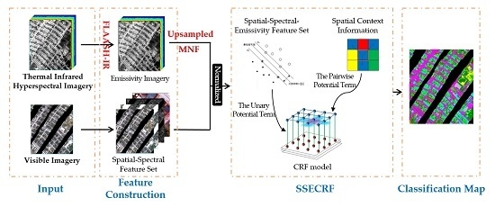
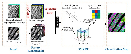
In this paper, in order to make full use of the spatial-spectral-emissivity information for precise land-cover classification, the SSECRF algorithm is proposed to integrate the emissivity information retrieved from the thermal infrared hyperspectral imagery and the spatial and spectral information from the visible data. The emissivity and the spatial-spectral feature set are fused in the SSECRF algorithm using different potentials. The main procedure of the proposed method is illustrated in Figure 3. Firstly, the emissivity information is retrieved from the thermal infrared hyperspectral imagery data, and is upsampled to the same spatial resolution as the visible data. The spatial-spectral feature set is then constructed by extracting the different features from the visible data. Furthermore, the unary potential is modeled by integrating the emissivity and the spatial-spectral feature set, and the pairwise potential is modeled to consider the spatial interactions of the visible data in the neighborhood pixels. The final classification map is obtained when the SSE energy function is minimized.
3.2.1. Feature Extraction from the Thermal Infrared Hyperspectral Imagery
1. Emissivity retrieval from the thermal infrared hyperspectral imagery
The emissivity retrieved from the thermal infrared hyperspectral imagery is often seen as an indicator of material composition, i.e., the intrinsic property description of natural materials [20]. The emissivity information can help us to classify and identify minerals more accurately. In this paper, the FLAASH-IR [19] algorithm is used to transfer the raw radiance value of thermal infrared hyperspectral imagery to emissivity. The algorithm suppresses the influence of the atmosphere in the radiance spectra, and it can obtain a competitive emissivity result from the thermal infrared hyperspectral imagery.
2. Feature Dimensionality Reduction for the Emissivity Imagery
PCA is widely used for feature dimensionality reduction in remote sensing imagery preprocessing, and it can be described as a multidimensional orthogonal linear transformation method based on statistical features. However, the PCA transform is sensitive to image noise [36], i.e., a principal component with a large amount of information may have a lower signal-to-noise ratio. Therefore, it is not the best method to transfer the emissivity imagery from a high-dimensional feature space to a lower one. The minimum noise fraction (MNF) transform, as proposed by Green et al. [37], consists of principal component analysis with two stacking treatments. The noise in the transformation process has unit variance, and the band is not relevant, so the MNF transform is superior to the PCA transform [38].
3.2.2. Multi-Feature Extraction from the Visible Imagery
In general, the texture, spatial, and object-based features are extracted to complement the spectral information. In this paper, the VDVI image, texture images, spectral feature, and object-based spatial image are used to make up the feature map.
1. Spectral Feature
Although visible images are lacking in abundant spectral information, they can be used for the identification of objects that have a large difference in spectral properties. The spectral feature is expressed as follows:
where is defined as the spectral vector in site .
2. Visible Difference Vegetation Index (VDVI)
In remote sensing applications, there are more than 100 types of vegetation index (VI), but most of the vegetation indices are calculated with the visible and near-infrared bands, including the normalized difference vegetation index (NDVI), the ratio vegetation index (RVI), and the enhanced vegetation index (EVI). Considering the spectral characteristics of visible imagery, Wang et al. [18] referred to the construction principles and forms of the NDVI and proposed the comprehensive utilization of the red, green, and blue bands to generate the VDVI, which is calculated as follows:
where , , and are the digital number or reflectance values in the green, red, and blue bands for visible imagery.
3. Texture Feature
The texture feature of visible imagery plays a critical role in distinguishing the objects which have similar spectral features. A texture feature which considers the spatial relationship of pixels is the GLCM. The GLCM describes the texture of an image by calculating the frequency of the pixel pairs with specific values and in a specified spatial relationship occurring in the image, creating a GLCM, and then extracting statistical measures from this matrix. A total of 14 kinds of texture features are optional in remote sensing applications. In urban classification, the object shape and material properties of the ground objects are generally considered. The mean reflects the regularity of the texture. If the texture is disorganized and difficult to describe, the value will be small. Contrarily, the texture is regular and easy to describe when the value is larger. The homogeneity measures the local gray uniformity of an image. If the texture of different regions lack of changes and the local gray level of the image is uniform, then the homogeneity will be larger. The contrast directly reflects the brightness contrast of a pixel and its neighboring regions. If the element far from the diagonal has a greater value, i.e., the brightness of this image change quickly, then the contrast will be larger. Meanwhile, the contrast reflects the clarity and texture depth of the image. Therefore, in the proposed multi-feature fusion framework, the texture features of mean, homogeneity, and contrast are obtained to describe the spatial texture feature.
The features can be represented as the following forms:
4. Object-Based Feature
Visible imagery has abundant spatial, texture, and spectral characteristics. In order to alleviate the effect of the within-class spectral variability and noise in the feature space, a segmentation prior is essential. Generally speaking, object-based feature extraction can be divided into object construction and feature extraction. The quality of the segmentation is related to the scale of the mergence and segmentation options, and the performance of the segmentation has a direct influence on the classification map. Considering the distribution of the land-cover types and the description rules of the spatial attributes, compactness, roundness, form factor, and rectangular fit are defined as the object-based features in our method. The object-based features we extract from the visible image can be shown as:
where denotes the pixel site of the image, and is the optimum scale of the mergence and segmentation in the above formula.
3.2.3. Construction of the Spatial-Spectral-Emissivity (SSE) Feature Set
For visible imagery, the digital number (DN) value ranges from 0 to 255, but the emissivity value varies from 0 to 1, and the other feature information changes from 0 to 0.0001, etc. If all the original feature images are integrated directly, some of the characteristics will have an exaggerated influence, while some will be completely ignored. Normalization preprocessing of the feature images can sum up the statistical distribution to uniform samples and does not change the nature of the image. In view of this situation, it is necessary to balance the contribution degree of each feature map to the final fused image with the following formula:
where records the feature value at site , and and represent the maximum and minimum feature values of the whole feature image. The SSE feature set can be written as a vector:
3.2.4. Classification Based on SSECRF
As noted in Section 2, in the remote sensing imagery classification task, the most widely used model is the pairwise CRF model, which can be written as a sum of the unary potential term and pairwise potential term. It is equivalent to the Gibbs energy in Equation (3), where is the unary potential term and is the pairwise potential term. The latter item is defined on the local neighborhood of site . The non-negative constant λ is the adjusting parameter of the pairwise potential term, which weighs the influence of these two potential terms. After modeling the basic framework, how to model the potential function needs to be considered, as well as optimizing the energy function to find the final class labels.
1. SSECRF Energy Function
Here, we redefine Equation (3) in the SSECRF algorithm, so the unary potential can be written as , integrating the SSE feature obtained in the multi-feature extraction from the visible and thermal infrared hyperspectral imagery data, where is an observation field representing the SSE feature set, and the pairwise potential is , representing the spatial interaction in the visible imagery, where is also an observation field representing the spectral and spatial contextual information of the visible imagery. Therefore, the well-studied pairwise CRF can be reformulated with the sum of the unary and pairwise potentials, and the energy function can be shown as follows:
2. Unary Potential
The unary potential is modeled to integrate the emissivity information with the spatial-spectral feature set from the visible imagery. The complementary information in the two types of imagery is then used to conduct the identification of land-cover types. The unary potential models the relationship between the label image and the observed image. In other words, it considers the calculation cost of each pixel belonging to each specific class. Therefore, under the condition that the given image feature vector is known, the classification algorithm can be used to calculate the probability estimation of each pixel independently. Here, the “given image feature vector” is defined as the “fusion image”, which makes full use of the emissivity and spatial-spectral feature set of the visible imagery to help discriminate the various land-cover types. Therefore, the different features that are sensitive to the different ground classes are considered in the classification task. The unary potential can be defined as [39]:
where represents the feature vector consisting of the emissivity and other feature information at site , and is the probability of pixel belonging to class label , based on the feature vector. Minimizing the unary potential function can be considered as image classification. Due to the SVM algorithm being known to perform well in remote sensing imagery classification in the case of limited samples [40], the probability estimation is obtained by SVM.
3. Pairwise Potential
Due to the spectral variability and image noise in the visible imagery, the spectral vectors of adjacent pixels in the homogeneous regions of the image are not equal. Based on the spatial correlation of the ground features, adjacent pixels can usually be assumed to be the same object. The pairwise potential is modeled to consider the a-priori smoothness and the spatial patterns of the land-cover types, such as the shape and size information, etc. The abundant spatial features of the visible imagery play an important role in identifying the types of certain pixels. In our algorithm, the pairwise potential energy simultaneously considers the observed image and the label image to model the spatial-contextual relationship of each pixel and its associated neighborhood [41]. This can ensure that the adjacent pixels in the homogeneous areas obtain the same label, while retaining the boundaries of adjacent areas at the same time. The pairwise potential function take the form of [39,42] and can be defined as:
where models the spatial interaction of adjacent pixels and , measuring the difference in appearance between them, and where is the Euclidean distance between the adjacent pixels, and and represent the spectral feature vector in sites and , respectively. The parameter is set to the mean square deviation of the feature vector variance between the adjacent pixels in the image, which is written as , where indicates the mean calculation over the image.
The pairwise potential energy makes it possible to consider the spatial interaction between local pixels in the classification. When minimizing the energy function , it is still expected to retain the continuity of the labels and make the adjacent pixels in the homogeneous regions have the same label in the classification map.
4. Inference Algorithm
After the construction of the potential function in SSECRF, it is critical to optimize the energy function and obtain the final labels. The inference algorithm is designed to predict the optimal class labels, which correspond to calculating the minimum value of the energy function. A number of different approximate inference algorithms have been put forward to obtain the optimal labels, including iterated conditional modes and graph cuts. In this paper, the α-expansion algorithm based on graph cuts [43] is used for the multi-class labeling problem. A local search strategy is designed to solve the problem of the small moving space easily falling into local optima for the energy function satisfying the multivalued variables. The local search strategy of the algorithm continues to calculate the global minimum values in the binary labeling problem through the graph cuts algorithm in the loop. The graph cuts based on the α-expansion algorithm can be considered to simplify the multi-class labeling problem to a sequence of optimization subproblems with binary labels, which can be easily optimized by the graph-cut method. Also, the α-expansion inference algorithm is described in the following. The current label is initialized as , and the α-expansion algorithm gives each pixel the following choices: keeping the current label unchanged or converting to a specific label . All the pixels of the image make a choice simultaneously; the algorithm has exponential-level moving space with respect to any particular α, which ensures that the algorithm has a strong local minimum property. For particular α, the binary labeling problem in the α-expansion algorithm can obtain the optimal value through the graph cuts algorithm to optimize the objective function .
4. Experiments and Analysis
4.1. Experimental Description
The multi-feature set extracted from the visible imagery and the emissivity retrieved from the thermal infrared hyperspectral imagery using FLAASH-IR were used to form the SSE feature set. In this paper, the VDVI is calculated with the red and green band from the visible image. The GLCM texture, that is Haralick measures (mean, homogeneity, contrast), is used to characterize the texture information with a window size 3, considering the time efficiency when calculating the GLCM texture of a large imagery. For the object-based feature, the scale of mergence and segmentation is selected based on some additional experiments. The object-based feature image is obtained with the different scales; then, they were input to the classifier to get a classification map. A high classification accuracy represents the optimal scales. In the paper, the scale of mergence and segmentation is (80, 90). At the same time, the emissivity information was resampled to the same resolution with the visible imagery and the first five components of the MNF was used in the SSE feature set. All the classification experiments were conducted by supervisor classification method using the training samples, and these samples are shown in Figure 1c, and the classification results were assessed by calculating the overall accuracy and kappa coefficient using the test samples shown in Figure 1d.
4.2. Experimental Results and Analysis
Experiments were undertaken to verify the classification performance of the proposed SSECRF algorithm. At the same time, the SSECRF result was compared with the result of the SSE feature set input into the SVM classifier, and the SSECRF result was also compared with the other existing methods.
4.2.1. Validity Analysis of the Multi-Feature Fusion Framework for the High-Resolution Visible Imagery
In order to verify the effectiveness of the features extracted from the visible imagery (VDVI, texture feature, and object-based feature map), the features were individually fused with the visible data and classified by the SVM algorithm.
From Table 2, it can be seen that the use of only the visible imagery can obtain a desirable classification result. However, the overall accuracy (OA) and kappa coefficient are improved greatly using the composite of VIS + Tex. + Obj. + VDVI (i.e., the spatial-spectral feature set), indicating that the extracted features are effective in the classification task.
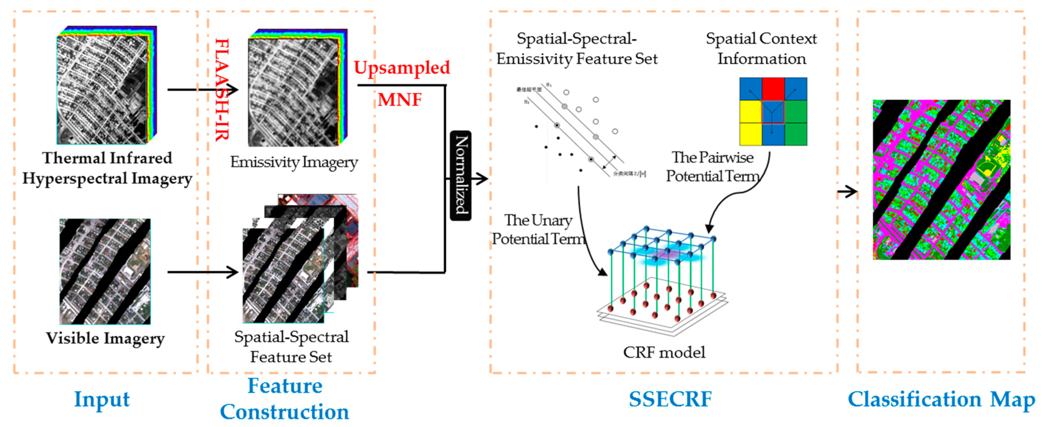
After separate fusion of some of the features extracted from the visible data, the accuracy of certain classes increases or decreases slightly, as shown in Figure 4. This indicates that some combinations of feature maps are sensitive to specific classes. For instance, when adding the object-based feature in visible imagery, trees and grey roofs can be identified well, but the accuracy of vegetation is decreased. Finally, it can be expected that the OA will be further improved by integrating the emissivity information retrieved from the thermal infrared hyperspectral imagery data.
4.2.2. Validity Analysis for the SSE Feature Set
The emissivity imagery and the raw thermal infrared hyperspectral imagery data were both upsampled to the same high resolution as the visible data. The first five components of these two images were used for the integration with the spatial-spectral feature set from the visible imagery, respectively, and they can be represented as the SSE feature set and the SSR feature set (integrating the raw radiance image with the spatial-spectral feature set). The SSE feature set was constructed based on the retrieved emissivity information from the raw thermal infrared hyperspectral imagery data. The constructed feature sets were input into the SVM classifier separately, and the confusion matrices were obtained using the test samples. As shown in Table 3 and Table 4, by the use of the SSE feature set, the OA is increased from 91.7864 to 91.8101, and the kappa is increased from 0.8775 to 0.8779. It can be revealed that the classification results obtained using the SSE feature set improve the identification of the bare soil compared with the results obtained using the SSR feature set, and the confusion between bare soil and red roof is improved. In addition, the accuracies of the roof classes are improved slightly when using the SSE feature set. Overall, the results show that the construction of the SSE feature set leads to a better classification performance.
4.2.3. Validity Analysis of the SSECRF Algorithm
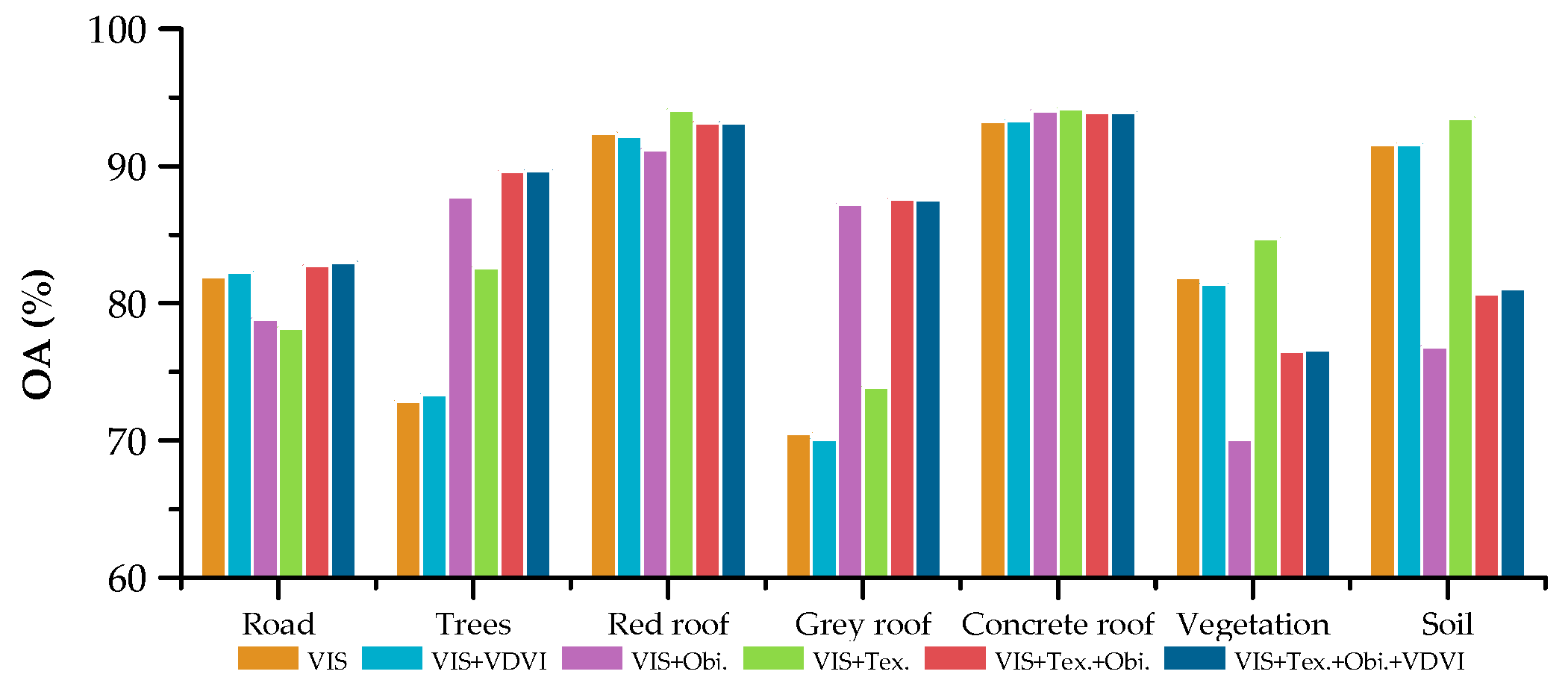
For the classification task, the visual performance is of importance for the proposed method, so the final classification map obtained by the SSECRF algorithm is shown in Figure 5. The classification map exhibits a good appearance in some classes, except for the misclassification between trees and vegetation. It preserves the more useful information and achieves a complete shape feature with fewer meaningless regions and less salt-and-pepper classification noise. However, the over-fitting phenomenon can be observed in the road area. On the whole, the proposed SSECRF algorithm shows a pleasing visual performance.
At the same time, the quantitative confusion matrix can also reflect the performance of the classification result. The given test samples were used to evaluate the effectiveness of the proposed method, and the corresponding quantitative results are reported in Table 5. The class accuracies are all more than 90%, except for the trees and vegetation, which are confused. In summary, the quantitative evaluation result shows an effective classification performance after the fusion of the visible and thermal infrared hyperspectral imagery by SSECRF.
In the proposed algorithm, the SSE feature set is used to model the unary potential. In Section 4.2.2, the SSE feature set was input into SVM (SSE-SVM) to obtain the classification map, obtaining a result that was better than the results obtained using the SSR feature set. From the confusion matrices, it can be seen that CRF performs well in distinguishing all the classes, especially grey roof, vegetation, and bare soil.
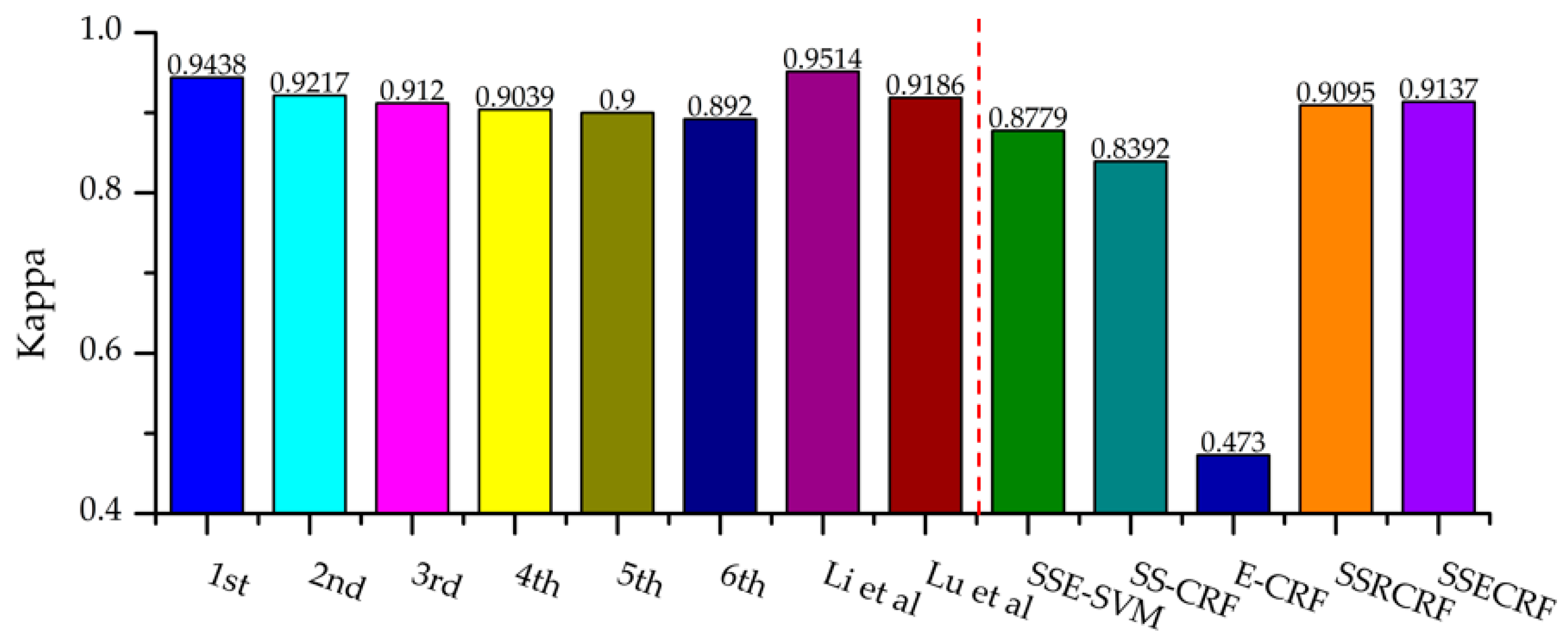
At the same time, other experiments were conducted with SSECRF using the different feature sets to model the unary potential term. The spatial-spectral feature set from the visible imagery and the emissivity information used separately in the SSECRF algorithm are denoted as SS-CRF and E-CRF. A comparison of the subset classification maps is shown in Figure 6, where it can be observed that the SSE-SVM results contain much salt-and-pepper classification noise, and the SS-CRF and E-CRF results lose much detailed information. At the same time, the kappa values of the classification results are compared in Figure 7, which are all lower than the results obtained with SSECRF using the SSE feature set.
In order to verify both the effectiveness of the proposed SSECRF algorithm and the effectiveness of using the emissivity information to improve the classification accuracy, the kappa coefficients of the top-six classification results [44] in the 2014 Data Fusion Contest, the published classification results obtained with other methods, and the results of the proposed algorithm are compared in Figure 7. All the experiments were undertaken under the same conditions, i.e., the same training samples and test samples. The comparison shows that the classification results of the proposed method show a competitive advantage, but the results are not as good as the results of 1st place in the 2014 Data Fusion Contest and the algorithms proposed later. It is possible that the results of the proposed method could be improved when the misclassification of vegetation and trees is solved.
4.3. Sensitivity Analysis
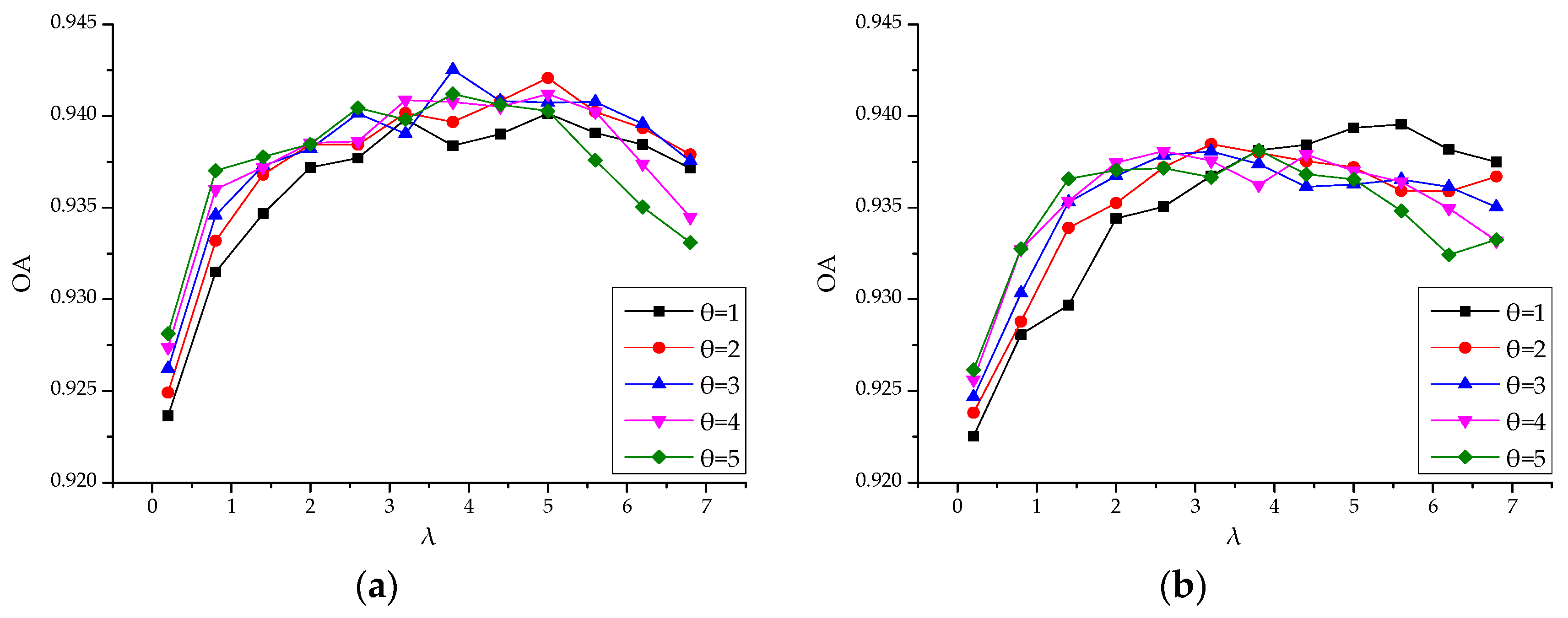
The final experimental results demonstrate that the SSECRF algorithm efficiently integrates the respective advantages of the visible and thermal infrared hyperspectral imagery, and it shows a good performance in land-cover classification. However, two parameters λ and θ are needed, as described in the SSECRF energy function , which have an effect on the final classification result. These two parameters mainly relate to the spatial interactions in the pairwise potential function. An additional 120 experiments were conducted to make a sensitivity analysis. Parameter λ ranged from 0.2 to 6.8 with a step length of 0.6, and parameter θ varied from 1 to 5 with an interval of 1. Figure 8 shows the relationship between the OA and the parameter selection in the SSECRF algorithm.
For Figure 8a, the classification map was obtained integrating the spatial-spectral feature set from the visible imagery and the emissivity from the thermal infrared hyperspectral imagery by the SSECRF algorithm. The OA from 60 experiments exhibits a tendency to first rise and then decrease slightly as parameter λ increases when keeping θ unchanged. It can be concluded that parameter λ can make full use of the spatial-contextual information in the neighborhood, reducing the influence of the salt-and-pepper noise in the classification to improve the accuracy. However, when parameter λ is increased beyond a certain value, the effect of the spatial smoothing is too much, resulting in over-smoothing, so that the accuracy shows a downward trend. For parameter θ, which is a parameter in the spatial smoothing term, it has a similar function to parameter λ. In addition, it has a fine-tuning effect on the classification accuracy when keeping parameter λ constant.
For Figure 8b, the same experimental conditions were repeated with the same ranges of the two parameters λ and θ, but the emissivity feature was replaced by raw radiance data of the thermal infrared hyperspectral imagery when constructing the unary potential in SSECRF, and another 60 experiments were conducted. It is worth noting that the OA of the best classification result is no better than the best classification result obtained with the SSE feature set. Therefore, it can be proved that SSECRF is a relatively stable algorithm, and the classification performance changes regularly with the change of the parameters.
5. Conclusions
In this paper, the SSECRF algorithm has been proposed to efficiently integrate visible imagery and thermal infrared hyperspectral imagery for land-cover classification. The existing methods of fusing the visible and thermal infrared hyperspectral imagery do not take into account the emissivity information, and only the raw radiance information of the thermal infrared hyperspectral imagery is employed. The SSECRF algorithm considers the spatial-contextual information and spectral variability, and makes full use of the emissivity to improve the final classification result. Firstly, features extracted from these two types of imagery are used to fuse the SSE feature set. The unary potential and the pairwise potential are then modeled as the SSE energy function. The unary potential is modeled to integrate the emissivity information with the spatial-spectral feature set from the visible imagery, and the pairwise potential is modeled using a spatial smoothing term to make full use of the spatial-contextual information. Two parameters λ and θ have an influence on the pairwise potential term, and the choice of parameters directly determines the classification results.
The experiments undertaken in this study confirmed that the proposed SSECRF algorithm can efficiently integrate the visible and thermal infrared hyperspectral data, and a satisfactory classification map can be obtained, where the spatial, spectral, and emissivity information are all considered to obtain a better classification result. The final classification map shows a good performance and OA, especially for certain classes, such as roads and bare soil, proving that the SSECRF algorithm is effective.
In the future, strategies will be investigated that could be applied in distinguishing the vegetation and roofs class more accurately. Also, the temperature information retrieved from the thermal infrared hyperspectral imagery will be also considered.
Acknowledgments
This work was supported by National Natural Science Foundation of China under Grant Nos. 41622107, 41771385 and 41371344, National Key Research and Development Program of China under Grant No. 2017YFB0504202, and Natural Science Foundation of Hubei Province in China under Grant No. 2016CFA029. The authors would like to thank Telops Inc. (Quebec City, Quebec, Canada) for acquiring and providing the data used in this study, the IEEE GRSS Image Analysis and Data Fusion Technical Committee and M. Shimoni (Signal and Image Centre, Royal Military Academy, Belgium) for organizing the 2014 Data Fusion Contest, the Centre de Recherche Public Gabriel Lippmann (CRPGL, Luxembourg) and M. Schlerf (CRPGL) for their contribution of the Hyper-Cam LWIR sensor, and M. De Martino (University of Genoa, Genoa, Italy) for her contribution in data preparation. The authors also want to thank Telops Inc. (Quebec City, Quebec, Canada) for providing the emissivity map retrieved using Spectral Sciences Inc.’s FLAASH-IR in our experiment.
Author Contributions
All the authors made significant contributions to the work. Yanfei Zhong, Tianyi Jia and Ji Zhao designed the research and analyzed the results. Xinyu Wang and Shuyin Jing provided advice for the preparation and revision of the paper.
Conflicts of Interest
The authors declare no conflict of interest.
References
- Cihlar, J. Land cover mapping of large areas from satellites: Status and research priorities. Int. J. Remote Sens. 2000, 21, 1093–1114. [Google Scholar] [CrossRef]
- Zhong, Y.; Cao, Q.; Zhao, J.; Ma, A.; Zhao, B.; Zhang, L. Optimal Decision Fusion for Urban Land-Use/Land-Cover Classification Based on Adaptive Differential Evolution Using Hyperspectral and LiDAR Data. Remote Sens. 2017, 9, 868. [Google Scholar] [CrossRef]
- Zhu, Q.; Zhong, Y.; Zhang, L.; Li, D. Scene Classification Based on Fully Sparse Semantic Topic Model. IEEE Trans. Geosci. Remote Sens. 2017, 55. [Google Scholar] [CrossRef]
- Haralick, R.M.; Shanmugam, K. Textural features for image classification. IEEE Trans. Syst. Man. Cybern. 1973, 6, 610–621. [Google Scholar] [CrossRef]
- Pesaresi, M.; Benediktsson, J.A. A new approach for the morphological segmentation of high-resolution satellite imagery. IEEE Trans. Geosci. Remote Sens. 2001, 39, 309–320. [Google Scholar] [CrossRef]
- Taubenböck, H.; Esch, T.; Wurm, M.; Roth, A.; Dech, S. Object-based feature extraction using high spatial resolution satellite data of urban areas. J. Spat. Sci. 2010, 55, 117–132. [Google Scholar] [CrossRef]
- Cheng, J.; Liang, S.; Wang, J.; Li, X. A stepwise refining algorithm of temperature and emissivity separation for hyperspectral thermal infrared data. IEEE Trans. Geosci. Remote Sens. 2010, 48, 1588–1597. [Google Scholar] [CrossRef]
- Riley, D.N.; Hecker, C.A. Mineral mapping with airborne hyperspectral thermal infrared remote sensing at Cuprite, Nevada, USA. In Thermal Infrared Remote Sensing: Sensors, Methods, Applications; Kuenzer, C., Dech, S., Eds.; Springer: Berlin, Germany, 2013; pp. 495–514. [Google Scholar]
- Fontanilles, G.; Briottet, X.; Fabre, S.; Lefebvre, S.; Vandenhaute, P.F. Aggregation process of optical properties and temperature over heterogeneous surfaces in infrared domain. Appl. Opt. 2010, 49, 4655–4669. [Google Scholar] [CrossRef] [PubMed]
- Liao, W.; Huang, X.; Van Coillie, F.; Gautama, S.; Pižurica, A.; Philips, W.; Liu, H.; Zhu, T.; Shimoni, M.; Moser, G. Processing of multiresolution thermal hyperspectral and digital color data: Outcome of the 2014 IEEE GRSS data fusion contest. IEEE J. Sel. Top. Appl. Earth Obs. Remote Sens. 2015, 8, 2984–2996. [Google Scholar] [CrossRef]
- Michaelsen, E. Self-organizing maps for fusion of thermal hyperspectral-with high-resolution VIS-data. In Proceedings of the 8th IAPR Workshop on Pattern Recognition in Remote Sensing (PRRS 2014), Stockholm, Sweden, 24 August 2014; pp. 1–4. [Google Scholar]
- Hasani, H.; Samadzadegan, F. 3D object classification based on thermal and visible imagery in urban area. In Proceedings of the International Archives of Photogrammetry, Remote Sensing and Spatial Information Sciences, Göttingen, Germany, 23–25 November 2015; Volume XL.1, pp. 287–291. [Google Scholar]
- Li, J.; Zhang, H.; Guo, M.; Zhang, L.; Shen, H.; Du, Q. Urban classification by the fusion of thermal infrared hyperspectral and visible data. Photogramm. Eng. Remote Sens. 2015, 81, 901–911. [Google Scholar] [CrossRef]
- Lu, X.; Zhang, J.; Li, T.; Zhang, G. Synergetic classification of long-wave infrared hyperspectral and visible images. IEEE J. Sel. Top. Appl. Earth Obs. Remote Sens. 2015, 8, 3546–3557. [Google Scholar] [CrossRef]
- Marwaha, R.; Kumar, A.; Kumar, A.S. Object-oriented and pixel-based classification approach for land cover using airborne long-wave infrared hyperspectral data. J. Appl. Remote Sens. 2015, 9, 095040. [Google Scholar] [CrossRef]
- Akbari, D.; Homayouni, S.; Safari, A.; Mehrshad, N. Mapping urban land cover based on spatial-spectral classification of hyperspectral remote-sensing data. Int. J. Remote Sens. 2016, 37, 440–454. [Google Scholar] [CrossRef]
- Samadzadegan, F.; Hasani, H.; Reinartz, P. Toward optimum fusion of thermal hyperspectral and visible images in classification of urban area. Photogramm. Eng. Remote Sens. 2017, 83, 269–280. [Google Scholar] [CrossRef]
- Wang, X.; Wang, M.; Wang, S.; Wu, Y. Extraction of vegetation information from visible unmanned aerial vehicle images. Trans. Chin. Soc. Agric. Eng. 2015, 31, 152–159. [Google Scholar]
- Adler-Golden, S.; Conforti, P.; Gagnon, M.; Tremblay, P.; Chamberland, M. Long-wave infrared surface reflectance spectra retrieved from Telops Hyper-Cam imagery. In Proceedings of the Algorithms and Technologies for Multispectral, Hyperspectral, and Ultraspectral Imagery XX, Baltimore, MD, USA, 5 May 2014; Volume 9088, p. 90880U. [Google Scholar]
- Sobrino, J.; Raissouni, N.; Li, Z.L. A comparative study of land surface emissivity retrieval from NOAA data. Remote Sens. Environ. 2001, 75, 256–266. [Google Scholar] [CrossRef]
- Gillespie, A.; Rokugawa, S.; Matsunaga, T.; Cothern, J.S.; Hook, S.; Kahle, A.B. A temperature and emissivity separation algorithm for advanced spaceborne thermal emission and reflection radiometer (ASTER) images. IEEE Trans. Geosci. Remote Sens. 1998, 36, 1113–1126. [Google Scholar] [CrossRef]
- Jin, M.; Liang, S. An improved land surface emissivity parameter for land surface models using global remote sensing observations. J. Clim. 2006, 19, 2867–2881. [Google Scholar] [CrossRef]
- Gagnon, M.A.; Tremblay, P.; Savary, S.; Duval, M.; Farley, V.; Lagueux, P.; Guyot, É.; Chamberland, M. Airborne thermal infrared hyperspectral imaging for mineral mapping. In Proceedings of the International Workshop on Advanced Infrared Technology & Applications, Pisa, Italy, 29 September–2 October 2015; pp. 83–86. [Google Scholar]
- Kastek, M.; Piątkowski, T.; Trzaskawka, P. Infrared imaging fourier transform spectrometer as the stand-off gas detection system. Metrol. Meas. Syst. 2011, 18, 607–620. [Google Scholar] [CrossRef]
- Neinavaz, E.; Darvishzadeh, R.; Skidmore, A.K.; Groen, T.A. Measuring the response of canopy emissivity spectra to leaf area index variation using thermal hyperspectral data. Int. J. Appl. Earth Obs. 2016, 53, 40–47. [Google Scholar] [CrossRef]
- Lafferty, J.; McCallum, A.; Pereira, F. Conditional random fields: Probabilistic models for segmenting and labeling sequence data. In Proceedings of the International Conference on Machine Learning (ICML), Williamstown, MA, USA, 28 June–1 July 2001; pp. 282–289. [Google Scholar]
- Kumar, S. Discriminative random fields: A discriminative framework for contextual interaction in classification. In Proceedings of the Ninth IEEE International Conference on Computer Vision, Nice, France, 13–16 October 2003; pp. 1150–1157. [Google Scholar]
- Zhong, P.; Wang, R. Jointly learning the hybrid CRF and MLR model for simultaneous denoising and classification of hyperspectral imagery. IEEE Trans. Neural Netw. Learn. Syst. 2014, 25, 1319–1334. [Google Scholar] [CrossRef]
- Zhong, P.; Wang, R. Learning conditional random fields for classification of hyperspectral images. IEEE Trans. Image Process. 2010, 19, 1890–1907. [Google Scholar] [CrossRef] [PubMed]
- Yang, M.Y.; Förstner, W. A hierarchical conditional random field model for labeling and classifying images of man-made scenes. In Proceedings of the IEEE International Conference on Computer Vision Workshops (ICCV Workshops), Barcelona, Spain, 6–13 November 2011; pp. 196–203. [Google Scholar]
- Wegner, J.D.; Hansch, R.; Thiele, A.; Soergel, U. Building detection from one orthophoto and high-resolution InSAR data using conditional random fields. IEEE J. Sel. Top. Appl. Earth Obs. Remote Sens. 2011, 4, 83–91. [Google Scholar] [CrossRef]
- Lv, P.; Zhong, Y.; Zhao, J.; Jiao, H.; Zhang, L. Change detection based on a multifeature probabilistic ensemble conditional random field model for high spatial resolution remote sensing imagery. IEEE Geosci. Remote Sens. Lett. 2016, 13, 1965–1969. [Google Scholar] [CrossRef]
- Zhao, J.; Zhong, Y.; Shu, H.; Zhang, L. High-resolution image classification integrating spectral-spatial-location cues by conditional random fields. IEEE Trans. Image Process. 2016, 25, 4033–4045. [Google Scholar] [CrossRef] [PubMed]
- Kumar, S.; Hebert, M. Discriminative random fields. Int. J. Comput. Vis. 2006, 68, 179–201. [Google Scholar] [CrossRef]
- Kohli, P.; Torr, P.H. Robust higher order potentials for enforcing label consistency. Int. J. Comput. Vis. 2009, 82, 302–324. [Google Scholar] [CrossRef]
- Wang, C.; Wu, H.C.; Principe, J.C. Cost function for robust estimation of PCA. In Proceedings of the SPIE 2760, Applications and Science of Artificial Neural Networks II, Orlando, FL, USA, 8 April 1996; pp. 120–127. [Google Scholar]
- Green, A.; Craig, M.; Shi, C. The application of the minimum noise fraction transform to the compression and cleaning of hyper-spectral remote sensing data. In Proceedings of the IGARSS’88: Remote Sensing—Moving towards the 21st Century/International Geoscience and Remote Sensing Symposium, Edinburgh, UK, 12–16 September 1988; Volume 3, p. 1807. [Google Scholar]
- Murinto, K.; Nur, R.D.P. Feature reduction using minimum noise fraction and principal component analysis transforms for improving the classification of hyperspectral image. Asia-Pac. J. Sci. Technol. 2017, 22, 1–5. [Google Scholar]
- Shotton, J.; Winn, J.; Rother, C.; Criminisi, A. Textonboost: Joint appearance, shape and context modeling for multi-class object recognition and segmentation. In Proceedings of the 9th European Conference on Computer Vision, Graz, Austria, 7–13 May 2006; pp. 1–15. [Google Scholar]
- Vapnik, V.; Cortes, C. Support-vector networks. Mach. Learn. 1995, 20, 273–297. [Google Scholar]
- Zhao, J.; Zhong, Y.; Zhang, L. Detail-preserving smoothing classifier based on conditional random fields for high spatial resolution remote sensing imagery. IEEE Trans. Geosci. Remote Sens. 2015, 53, 2440–2452. [Google Scholar] [CrossRef]
- Rother, C.; Kolmogorov, V.; Blake, A. Grabcut: Interactive foreground extraction using iterated graph cuts. ACM Trans. Graph. 2004, 23, 309–314. [Google Scholar] [CrossRef]
- Boykov, Y.; Veksler, O.; Zabih, R. Fast approximate energy minimization via graph cuts. IEEE Trans. Pattern Anal. 2001, 23, 1222–1239. [Google Scholar] [CrossRef]
- 2014 IEEE GRSS Data Fusion Classification Contest Results. Available online: http://www.grss-ieee.org/community/technical-committees/data-fusion/2014-ieee-grss-data-fusion-classification-contest-results (accessed on 30 August 2017).
Figure 1.
Experimental datasets. (a) The visible image. (b) Gray-scale representation of the thermal infrared hyperspectral image. (c) The training samples. (d) The test samples.
Figure 1.
Experimental datasets. (a) The visible image. (b) Gray-scale representation of the thermal infrared hyperspectral image. (c) The training samples. (d) The test samples.
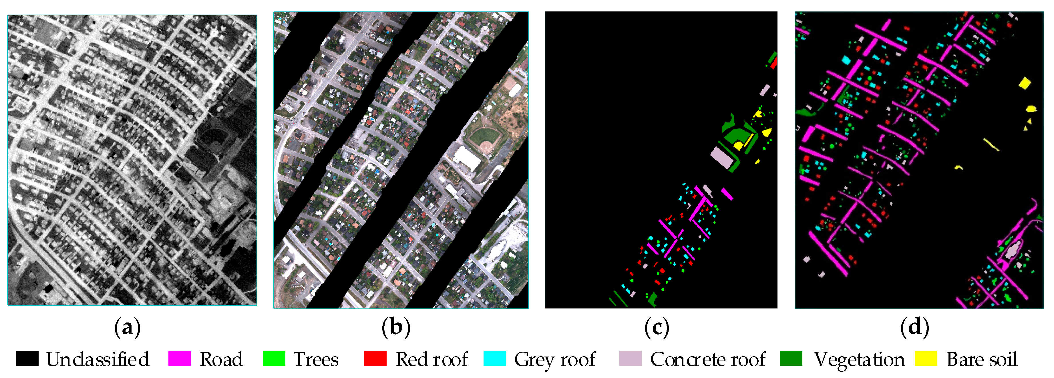
Figure 2.
Schematic diagram of conditional random fields (CRF) in image classification.
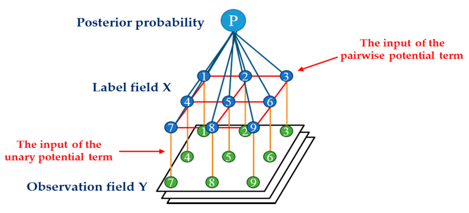
Figure 3.
The proposed Spatial-Spectral-Emissivity Land-Cover Classification Based on Conditional Random Fields (SSECRF) algorithm for fusing thermal infrared hyperspectral imagery and visible imagery.
Figure 3.
The proposed Spatial-Spectral-Emissivity Land-Cover Classification Based on Conditional Random Fields (SSECRF) algorithm for fusing thermal infrared hyperspectral imagery and visible imagery.

Figure 4.
Accuracy of the classification results for each class when fusing the visible imagery with different combinations of extracted features.
Figure 4.
Accuracy of the classification results for each class when fusing the visible imagery with different combinations of extracted features.

Figure 5.
The classification map obtained by the SSECRF algorithm. The representative areas are selected to show the details of the classification results in some specific classes. The black boxes 1 and 2 contain some roads, roofs and vegetation. A baseball field can be obviously seen in black box 3, and a large-area mixture of concrete roof and road is shown in black box 4.

Figure 6.
The subset classification results obtained by the SSECRF algorithm. The regions numbered 1, 2, 3 and 4 are the corresponding area subsets from the classification map in Figure 5.
Figure 6.
The subset classification results obtained by the SSECRF algorithm. The regions numbered 1, 2, 3 and 4 are the corresponding area subsets from the classification map in Figure 5.
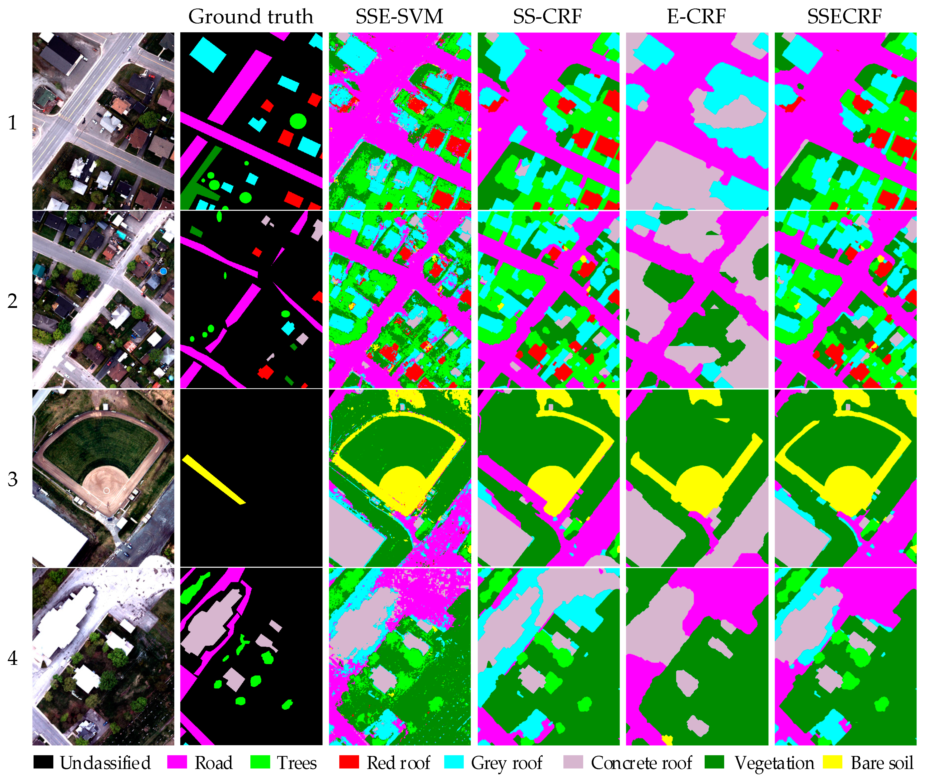
Figure 7.
The performance of the proposed SSECRF method compared with the existing methods, by kappa coefficient.
Figure 7.
The performance of the proposed SSECRF method compared with the existing methods, by kappa coefficient.

Figure 8.
Sensitivity analysis of parameters λ and θ. (a) The spatial-spectral feature set from the visible imagery and the emissivity from the thermal infrared hyperspectral imagery input into the SSECRF algorithm. (b) The spatial-spectral feature set from the visible imagery and the raw radiance of the thermal infrared hyperspectral imagery input into the SSECRF algorithm.


Table 1.
Class information for the datasets.
| Class | Training Samples | Test Samples |
|---|---|---|
| Road | 112,457 | 809,098 |
| Tree | 27,700 | 100,749 |
| Red roof | 46,578 | 136,697 |
| Grey roof | 53,520 | 142,868 |
| Concrete roof | 97,826 | 109,539 |
| Glass | 185,329 | 103,583 |
| Bare soil | 44,738 | 49,212 |
Table 2.
Accuracy assessment for the visible imagery with different combinations of extracted features, classified by support vector machine (SVM).
Table 2.
Accuracy assessment for the visible imagery with different combinations of extracted features, classified by support vector machine (SVM).
| VIS 1 | VIS + VDVI 2 | VIS + Obj. 3 | VIS + Tex. 4 | VIS + Tex. + Obj. | VIS + Tex. + Obj. + VDVI | |
|---|---|---|---|---|---|---|
| OA | 82.3218 | 82.4446 | 81.8945 | 81.7489 | 84.9826 | 85.1477 |
| Kappa | 0.7438 | 0.7452 | 0.7427 | 0.7401 | 0.7835 | 0.7857 |
1 VIS is visible imagery. 2 Visible Difference Vegetation Index (VDVI) is regarded as the VDVI feature map. 3 Obj. represents the object-based feature map. 4 Tex. represents the texture feature map calculated with the visible imagery.
Table 3.
Accuracy assessment of the classification results obtained with the SSR feature set.
| Road | Trees | Red Roof | Grey Roof | Concrete Roof | Vegetation | Bare Soil | |
|---|---|---|---|---|---|---|---|
| Road | 92.83 | 0.18 | 0.04 | 1.84 | 0.79 | 1.33 | 0.63 |
| Trees | 0.05 | 89.32 | 0.13 | 0 | 0.03 | 20.65 | 0 |
| Red roof | 0.01 | 0.02 | 96.57 | 4.31 | 0.01 | 0.01 | 7.39 |
| Grey roof | 5.24 | 0.31 | 2.77 | 91.02 | 3.55 | 0.06 | 0.25 |
| Concrete roof | 1.84 | 0 | 0.22 | 2.84 | 95.62 | 0.01 | 0.13 |
| Vegetation | 0 | 10.03 | 0.21 | 0 | 0 | 77.93 | 2.37 |
| Bare soil | 0.03 | 0.14 | 0.07 | 0 | 0 | 0.01 | 89.22 |
Table 4.
Accuracy assessment of the classification results obtained with the SSE feature set.
| Road | Trees | Red Roof | Grey Roof | Concrete Roof | Vegetation | Bare Soil | |
|---|---|---|---|---|---|---|---|
| Road | 92.9 | 0.19 | 0.03 | 2.26 | 0.72 | 1.16 | 0.5 |
| Trees | 0.04 | 89.23 | 0.1 | 0 | 0.01 | 19.97 | 0 |
| Red roof | 0.01 | 0.02 | 95.89 | 3.48 | 0.01 | 0.01 | 3.13 |
| Grey roof | 5.11 | 0.13 | 2.85 | 90.6 | 4.83 | 0.05 | 0.3 |
| Concrete roof | 1.83 | 0 | 0.11 | 3.65 | 94.37 | 0.01 | 0.39 |
| Vegetation | 0.01 | 10.35 | 0.12 | 0 | 0 | 78.46 | 1.96 |
| Bare soil | 0.1 | 0.07 | 0.91 | 0 | 0.05 | 0.35 | 93.71 |
Table 5.
Accuracy assessment of the classification map obtained by SSECRF.
| Road | Trees | Red Roof | Grey Roof | Concrete Roof | Vegetation | Bare Soil | |
|---|---|---|---|---|---|---|---|
| Road | 94.58 | 0.01 | 0 | 2.30 | 0.25 | 0.94 | 0.80 |
| Trees | 0 | 91.42 | 0.07 | 0 | 0 | 12.89 | 0 |
| Red roof | 0 | 0 | 97.39 | 3.04 | 0 | 0 | 0.21 |
| Grey roof | 4.80 | 0.03 | 2.44 | 94.66 | 4.19 | 0 | 0 |
| Concrete roof | 0.62 | 0 | 0 | 0 | 95.56 | 0 | 0 |
| Vegetation | 0 | 8.54 | 0 | 0 | 0 | 86.16 | 0.05 |
| Bare soil | 0 | 0 | 0.20 | 0 | 0 | 0 | 98.93 |
© 2017 by the authors. Licensee MDPI, Basel, Switzerland. This article is an open access article distributed under the terms and conditions of the Creative Commons Attribution (CC BY) license (http://creativecommons.org/licenses/by/4.0/).
Share and Cite
MDPI and ACS Style
Zhong, Y.; Jia, T.; Zhao, J.; Wang, X.; Jin, S. Spatial-Spectral-Emissivity Land-Cover Classification Fusing Visible and Thermal Infrared Hyperspectral Imagery. Remote Sens. 2017, 9, 910. https://doi.org/10.3390/rs9090910
AMA Style
Zhong Y, Jia T, Zhao J, Wang X, Jin S. Spatial-Spectral-Emissivity Land-Cover Classification Fusing Visible and Thermal Infrared Hyperspectral Imagery. Remote Sensing. 2017; 9(9):910. https://doi.org/10.3390/rs9090910
Chicago/Turabian StyleZhong, Yanfei, Tianyi Jia, Ji Zhao, Xinyu Wang, and Shuying Jin. 2017. "Spatial-Spectral-Emissivity Land-Cover Classification Fusing Visible and Thermal Infrared Hyperspectral Imagery" Remote Sensing 9, no. 9: 910. https://doi.org/10.3390/rs9090910
Note that from the first issue of 2016, this journal uses article numbers instead of page numbers. See further details here.