Response of Canopy Solar-Induced Chlorophyll Fluorescence to the Absorbed Photosynthetically Active Radiation Absorbed by Chlorophyll


1
Key Laboratory of Digital Earth Science, Institute of Remote Sensing and Digital Earth, Chinese Academy of Sciences, Beijing 100094, China
2
University of Chinese Academy of Sciences, Beijing 100049, China
*
Author to whom correspondence should be addressed.
Remote Sens. 2017, 9(9), 911; https://doi.org/10.3390/rs9090911
Submission received: 21 June 2017
/
Revised: 28 August 2017
/
Accepted: 28 August 2017
/
Published: 1 September 2017
(This article belongs to the Section Remote Sensing in Agriculture and Vegetation)
Abstract
:Solar-induced chlorophyll fluorescence (SIF), which can be used as a novel proxy for estimating gross primary production (GPP), can be effectively retrieved using ground-based, airborne and satellite measurements. Absorbed photosynthetically active radiation (APAR) is the key bridge linking SIF and GPP. Remotely sensed SIF at the canopy level () is only a part of the total SIF emission at the photosystem level. An SIF-based model for GPP estimation would be strongly influenced by the fraction of SIF photons escaping from the canopy (). Understanding the response of to the absorbed photosynthetically active radiation absorbed by chlorophyll () is a key step in estimating GPP but, as yet, this has not been well explored. In this study, we aim to investigate the relationship between remotely sensed and based on simulations made by the Soil Canopy Observation Photosynthesis Energy fluxes (SCOPE) model and field measurements. First, the ratio of the fraction of the absorbed photosynthetically active radiation absorbed by chlorophyll () to the fraction of absorbed photosynthetically active radiation absorbed by green leaves () is investigated using a dataset simulated by the SCOPE model. The results give a mean value of 0.722 for Cab at 5 μg cm−2, 0.761 for Cab at 10 μg cm−2 and 0.795 for other Cab content (ranging from 0.71 to 0.81). The response of to is then explored using simulations corresponding to different biochemical and biophysical conditions and it is found that is well correlated with . At the O2-A band, for a given plant type, the relationship between and can be approximately expressed by a linear statistical model even for different values of the leaf area index (LAI) and chlorophyll content, whereas the relationship varies with the LAI and chlorophyll content at the O2-B band. Finally, the response of to for different leaf angle distribution (LAD) functions is investigated using field observations and simulations; the results show that is larger for a planophile canopy structure. The values of the ratio of to are 0.0092, 0.0076 and 0.0052 μm−1 sr−1 for planophile vegetables/crops, planophile grass and spherical winter wheat, respectively, at the O2-A band. At the O2-B band, the ratios are 0.0063 , 0.0049 and 0.0033 μm−1 sr−1, respectively. The values of this ratio derived from observations agree with simulations, giving values of 0.0055 and 0.0068 μm−1 sr−1 at the O2-A band and 0.0032 and 0.0047 μm−1 sr−1 at the O2-B band for spherical and planophile canopies, respectively. Therefore, both the simulations and observations confirm that the relationship between and is species-specific and affected by biochemical components and canopy structure, especially at the O2-B band. It is also very important to correct for reabsorption and scattering of the SIF radiative transfer from the photosystem to the canopy level before the remotely sensed is linked to the GPP.
1. Introduction
Accurate estimation of the amount of carbon dioxide fixed by vegetation photosynthesis is a key component of the global carbon cycle and is also important for studies on ecosystem-climate interactions and ecosystem responses to extreme climate events [1,2]. There have been many approaches to estimating GPP (gross primary production) including the eddy covariance (EC) technique [3,4,5,6], process-based models [7,8,9] and LUE-models (light use efficiency models)based on the absorbed photosynthetically active radiation (APAR) absorbed by the canopy [10,11] or by green leaves [12,13]. However, the solar-induced chlorophyll fluorescence (SIF) emitted from vegetation chloroplasts is a more promising proxy for GPP than vegetation indices derived from reflectance data [14,15]. Recent instrumental developments in hyperspectral remote sensing make it possible to measure SIF using field spectrometers at ground level [16], airborne imaging spectrometers [17], and also satellite sensors including the high-spectral-resolution Japanese Greenhouse gases Observing SATellite (GOSAT) [18,19,20,21] and Orbiting Carbon Observatory 2 (OCO-2) [22] as well as the Scanning Imaging Absorption spectrometer for Atmospheric CHartograhY (SCIAMACHY) [23,24] and the Global Ozone Monitoring Experiment 2 (GOME-2) [25,26].
The simple linear response of the SIF to GPP at the large scale has been considered by many researchers. Based on the satellite-based Vegetation Photosynthesis Model (VPM) proposed by Xiao et al. [12], which includes the light use efficiency (LUE, ), the GPP can be calculated using Equation (1):
where PAR is the incident irradiance, is the fraction of absorbed photosynthetically active radiation absorbed by chlorophyll, is the light use efficiency and is the absorbed photosynthetically active radiation absorbed by chlorophyll [12,27,28]. Similarly, the total SIF originally emitted at the photosystem level (), a by-product of photosynthesis, can be expressed as
where is defined as the quantum yield for fluorescence (i.e., the fraction of APAR photons that are re-emitted from the photosystems as SIF photons). In this context, based on Equations (1) and (2), the GPP can be directly estimated using a linear model based on.
However, the remotely sensed SIF is only part of total SIF emitted from the chloroplasts within the leaves and is also not isotropic due to the upward radiation transfer path. As demonstrated by numerous observations and simulation results, the remotely sensed SIF at the canopy level () has a noticeable directional variation similar to that of the canopy reflectance in the solar principal plane [29]. In addition, the remotely sensed is strongly influenced by the effects of leaf and canopy structure, which affects the fluorescence reabsorption and the light penetration within the plant canopy [30]. Therefore, the remotely sensed can be similarly expressed as [14,28]
where is a parameter related to the optical properties of the canopy, which accounts for the fraction of SIF photons escaping from the photosynthesis level to the canopy level. It is determined by the canopy structure, the pigments that are present, the soil background, the illumination and the imaging geometries.
Therefore, if the ratio of to is constant, there should be a strong linear relationship between GPP and for a given vegetation type. Nevertheless, this linear relationship differs for different plant types due to the influence of the canopy structure or photochemical pathways [19,31,32,33,34].
As shown in Equations (1) and (3), APAR is the bridge linking SIF and GPP. Schlau-Cohen and Berry [35] found that the discrepancy and variation in the fluorescence quantum yield were both small under a range of illumination and stress conditions. So, the SIF signal may be a better proxy for estimating APAR. Based on diurnal and seasonal measurements made on a temperate deciduous forest [36] and crops [34], previous studies have demonstrated that SIF has a stronger correlation with APAR than with GPP. It is reasonable to assume that APAR is absorbed mainly by chlorophyll and also that the SIF is emitted by chlorophyll, which results in the significant correlation between SIF and APAR [14,37]. Therefore, understanding the mechanism underlying the link between directional SIF and is the key issue in interpreting the relationship between GPP and SIF. However, so far, this link has not been well explored.
In this paper, based on simulations made using the SCOPE (Soil Canopy Observation Photosynthesis Energy fluxes) model and field observations, we aim: (1) to investigate whether a reliable relationship exists between and and how this relationship is controlled by the canopy biochemical components and canopy structure—this includes the effect of the chlorophyll a + b content (Cab), leaf area index (LAI) and leaf angle distribution (LAD); and (2) to explore whether this relationship is different for signals at different bands. We hope this exploration of the relationship between and will assist in the estimation of GPP using remotely sensed SIF.
2. Materials and Methods
2.1. Simulation Data
The SCOPE model (version 1.61) was employed to simulate the SIF emission and APAR of the leaves and canopy with different biochemical and biophysical parameters under different environmental conditions. The inputs to the simulation experiment are listed in Table 1. The SCOPE model is a 1-D vertically integrated radiative transfer and energy balance model linking radiance observations at the top of the canopy with land surface characteristics, thus providing estimation of the amount of photosynthesis, leaf and canopy chlorophyll fluorescence and reflectance [38]. A range of values of the vegetation parameters, Cab, LAI, LIDFa (leaf angle distribution function) and LIDFb, as well as the geometrical parameters, solar zenith angle (SZA) and view zenith angle (VZA), were used in the simulation. Values of Cab ranging from 5 μg/cm2 to 80 μg/cm2 were used to represent the different chlorophyll levels. The LAI inputs were set from 0.5 to 7, indicating different levels of vegetation coverage. Six different leaf inclinations represented by combinations of LIDFa and LIDFb were used to represent different plant types. Different values of the SZA were set to correspond to different incident light conditions. All other SCOPE parameters were set to their default values.
2.2. Field Experiments
Seven independent field experiments were conducted in Beijing and in Sanya, Hainan Province, China. The distribution and location of three experimental sites are shown in Figure 1. The details are described below and also listed in Table 2. Corresponding to the spectral measurements, the auxiliary parameters measured simultaneously are also provided, including Cab, LAI and (the fractional cover of green vegetation).
Five experiments were carried out on winter wheat at the National Precision Agriculture Demonstration Base located at Xiao Tangshan (XTS) Farm, north of Beijing (11′N, 27′E). These experiments were conducted on two winter wheat varieties during two growth cycles, i.e., the 2015–2016 and 2016–2017 cycles. In the 2015–2016 cycle, the winter wheat (Triticum aestivum L.) was cultivated using conventional fertilizer and irrigation management and had a uniform growth status. Three diurnal experiments were conducted on 8, 9 and 18 April 2016 with the corresponding growth stages being the jointing, jointing, and booting stages, respectively. In each diurnal experiment, the upwelling canopy radiance and incident irradiance spectra were measured approximately every half hour from 8:30 to 17:00. In the 2016–2017 cycle, four fertilization rates were applied to two cultivated varieties of wheat (Lunxuan 167 and Jingdong 18). Two wheat varieties were cultivated in different columns next to each other on each field site. Four nitrogen fertilization treatments, i.e., different amount of carbamide were used: 585 kg ha−1 (N3), 390 kg ha−1 (N2), 195 kg ha−1 (N1), and no fertilization (N0). For each fertilization rate, three duplicates were also designed. Two experiments were conducted—one on 7 November 2016 and another on 8 December 2016—when the winter wheat was at the emergence and tillering stages, respectively.
Another diurnal spectral experiment was designed for gold coin grass (Lysimachia christinae Hance) and conducted on 18 December 2016 at Sanya Remote Sensing Satellite Data Receiving Station (18′N, 18′E) located in Sanya City, Hainan Province, China. The upwelling canopy radiance and incident irradiance spectra were measured approximately every 20 min from 8:00 to 17:00. The canopy structure was homogeneous and its coin-like leaves were oriented very close to ground.
A multi−species experiment was conducted on 18 December 2016 at Nanbin Farm (22′N, 10′E) in Sanya City, Hainan Province. The plant types at Nanbin farm included vegetables and crops such as potato, cabbage, cotton, rice and maize; their canopy structures were all planophile except for one observation made on rice.
Figure 2 displays three photographs of studied canopies at XTS Farm in November (left, winter wheat), Nanbin Farm (middle, cotton) and Sanya Station (right, gold coin grass). The canopy structure of winter wheat is spherical and the leaves are more erect compared with a planophile canopy. The Nanbin Farm experiment was carried out on a series of planophile crops that had horizontal leaves. The investigation of the diurnal dynamics of and at the Sanya Station focused on gold coin grass which had homogeneous, planophile leaves.
2.3. Details of the Spectral Measurements and SIF Retrieval Method
The canopy spectral measurements were made using a customized Ocean Optics QE Pro spectrometer (Ocean Optic, Inc., Dunedin, FL, USA) fitted with a field-of-view fiber optic that functions in the 645–805 nm spectral range with a full-width-at-half-maximum (FWHM, i.e., spectral resolution (SR)) of 0.31 nm, a spectral sampling interval of 0.155 nm and a peak signal-to-noise ratio (peak SNR) >1000. Canopy radiance measurements were taken by averaging 50 scans with an optimized integration time to weaken the influence of noise, and a dark current correction was applied to each spectral measurement. The canopy spectra were measured at a height of about 130 cm above the canopy for nadir observation. A BaSO4 calibration panel was used to measure the incoming solar irradiance. For all measurements, a relatively homogeneous view size of about 1 m × 1 m was selected. The weather was sunny and stable during all of the above experiments.
The SIF is a re-emitted signal corresponding to only a small amount of the reflected radiance and about 1% of the total light absorbed. It has two peaks at 685 nm and 740 nm. The SIF signal overlaps with the reflected light and needs to be separated out at the Fraunhofer lines or strong atmospheric absorption bands as, here, the incident irradiance is comparable to the amount of emitted fluorescence [39]. In this study, for the QE Pro spectral measurements, the O2-A (761 nm) and O2-B (688 nm) oxygen absorption bands were used to retrieve the far-red and red SIF, respectively, based on the 3FLD (3 band Fraunhofer Line Depth) method [40].
The 3FLD assumes that the variation in the SIF and in the reflectance are linear over the spectral range used. The single reference channel used in the standard FLD method (sFLD) for the incident irradiance and upwelling radiance is replaced by the weighted average of two channels at the left and right shoulders of the absorption band. Liu et al. [16] assessed the FLD-based SIF retrieval methods for different spectral specifications and showed that the 3FLD method was more accurate than the standard FLD method and also more robust than the improved FLD method proposed by Alonso et al. [41]. Therefore, we adopted the 3FLD method for retrieval in this study. The shoulder wavebands of the 3FLD method were determined according to Liu et al. [16,42]. In the case of the O2-A band, this corresponds to wavelengths of 757.92 nm, 760.72 nm and 768.87 nm for the bands corresponding to the left shoulder of the absorption feature, within the absorption feature and right shoulder of the absorption feature, respectively; for the O2-B band, it corresponds to wavelengths of 686.44 nm, 687.09 nm and 688.23 nm, respectively.
2.4. Measurement of and
The accurate measurement of the fraction of absorbed photosynthetically active radiation absorbed by green leaves () is a critical step in the estimation of . An in situ measurement method for low canopy vegetation based on a digital camera and reference panel was presented by Liu et al. [43] and has proved to be an effective solution for low canopy vegetation. Using this method, is given by
where and are the incident and reflected (including all exposed components) photosynthetically active radiation (PAR) derived from the DN values of the digital photograph. and are the PAR absorbed by the exposed background (including non-photosynthetic components) and the vegetation-covered background respectively. In green leaves, photosynthesis starts with the absorption of PAR, mainly by chlorophyll [30]. The absorption of APAR by green leaves is mostly due to the chlorophyll content. There is a linear correlation between and :
where k is the ratio of to . Then can be calculated based on Equation (6):
3. Results
3.1. The Relationship between and
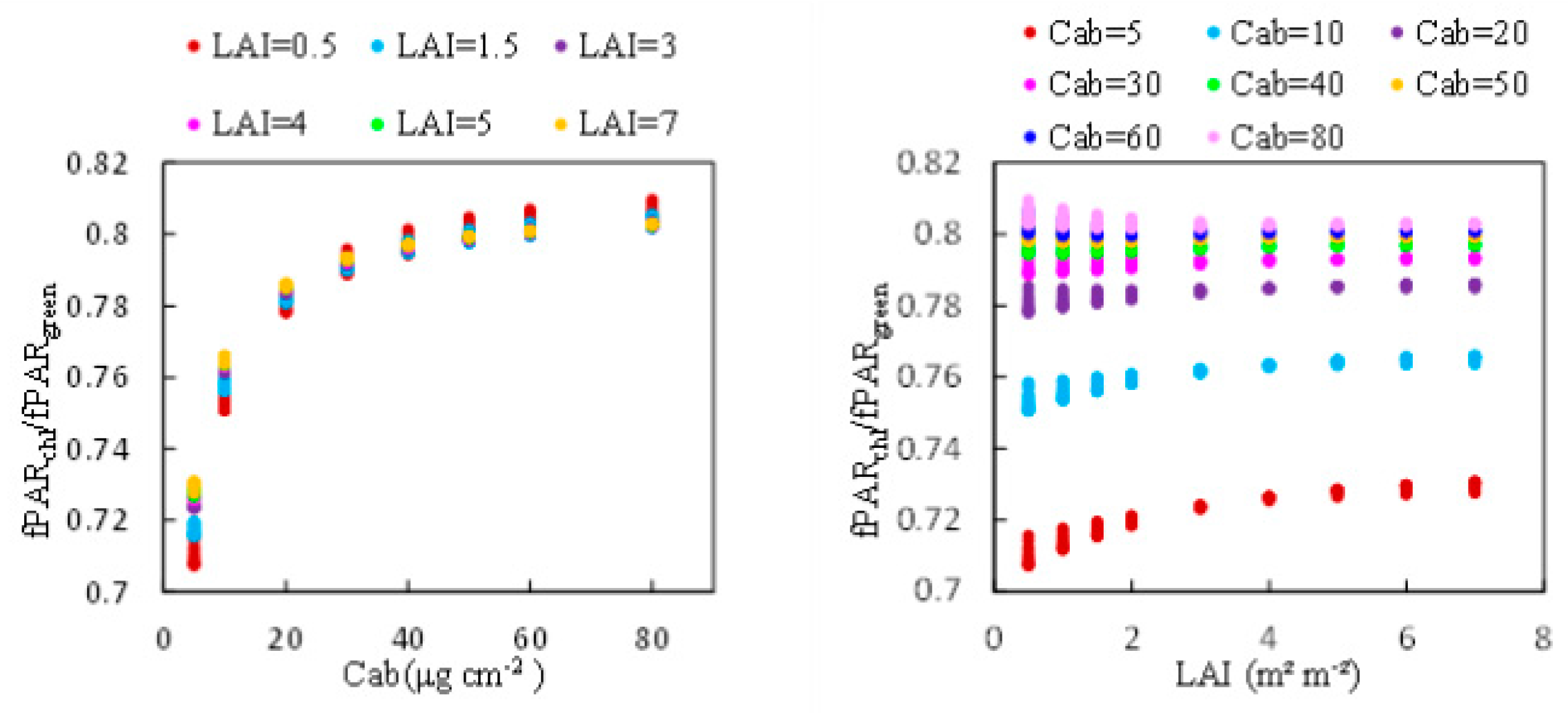
The ratio of to was determined for canopies with different LAI and Cab based on the simulation dataset described in Table 1. The results are illustrated in Figure 3 and there are 88 and 66 model runs in the subplot a and b (including 11 variations of SZA in each figure), respectively. The results show a mean value of 0.722 for Cab at 5 μg cm−2 and 0.761 for Cab at 10 μg cm−2 and 0.795 for other Cab content, with a range of 0.71 to 0.81. The ratio increases with increasing chlorophyll content but there is almost no change as LAI increases. Based on these results, the values (see Equation (5)) of 0.722 for Cab at 5 μg cm−2 and 0.761 for Cab at 10 μg cm−2 and 0.795 for other Cab content (ranging from 0.71 to 0.81) were subsequently used for the calculation of based on the field observations.
3.2. The Relationship between and Based on the Simulated Data
3.2.1. Effect of Chlorophyll Content on the Relationship between and
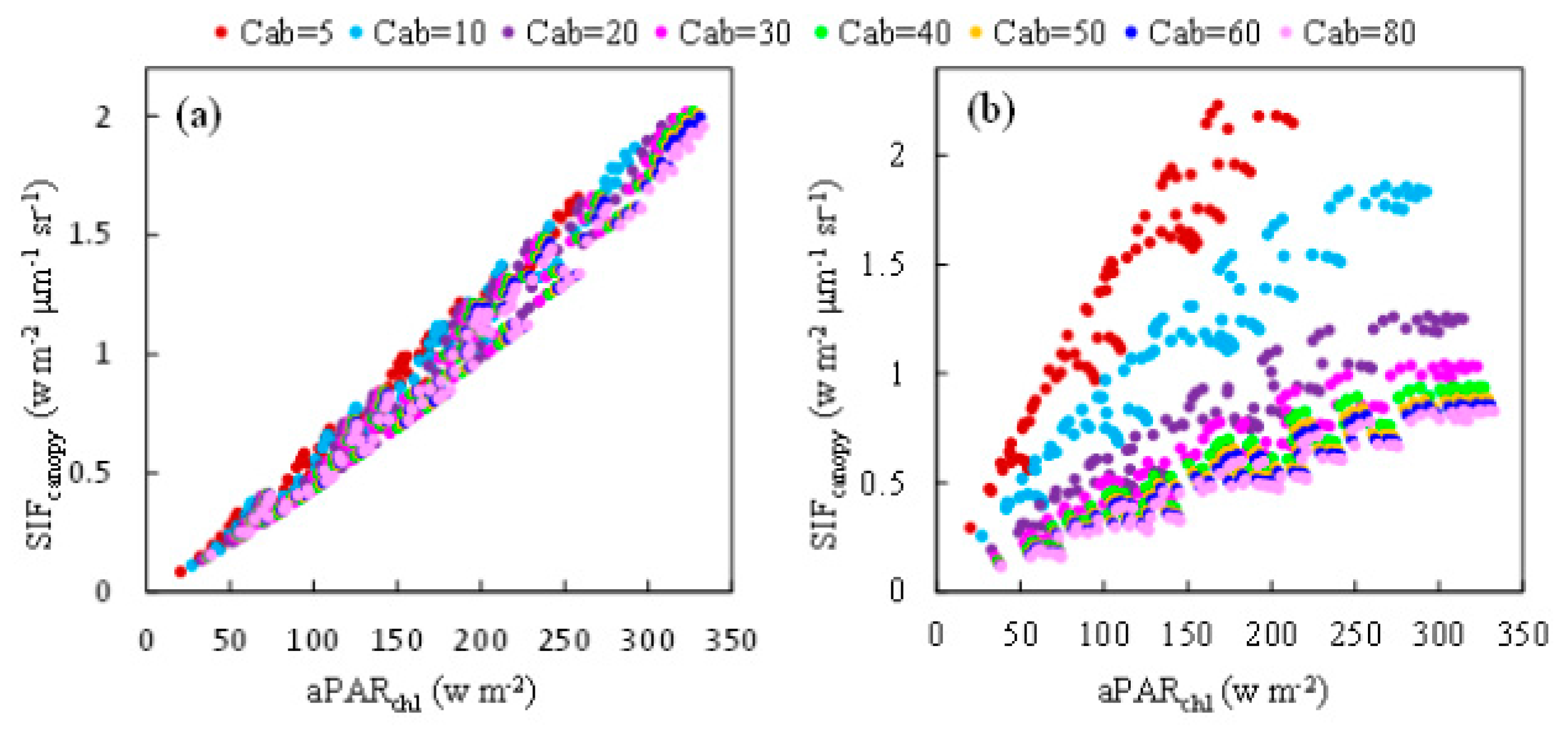
Simulated data representing canopies with different values of chlorophyll content but the same leaf angle distribution function (Spherical: LIDFa = −0.35, LIDFb = −0.15) was selected to investigate the relationship between and at the O2-A and O2-B bands, illustrated in Figure 4. For the O2-A band (Figure 4a), shows a strong linear relationship with for all the values of Cab tested, which means this linear relationship is almost independent of the chlorophyll content. It can be concluded that at the O2-A band is primarily driven by . For the O2-B band, when the results for different values of Cab are plotted, the relationship between and exhibits a pronounced wing-like shape (Figure 4b). The slope of to is sensitive to the Cab content, decreasing when Cab increases and becoming almost saturated when Cab is bigger than 40 μg/cm2. These results are similar to those found by Zhang et al. [33].
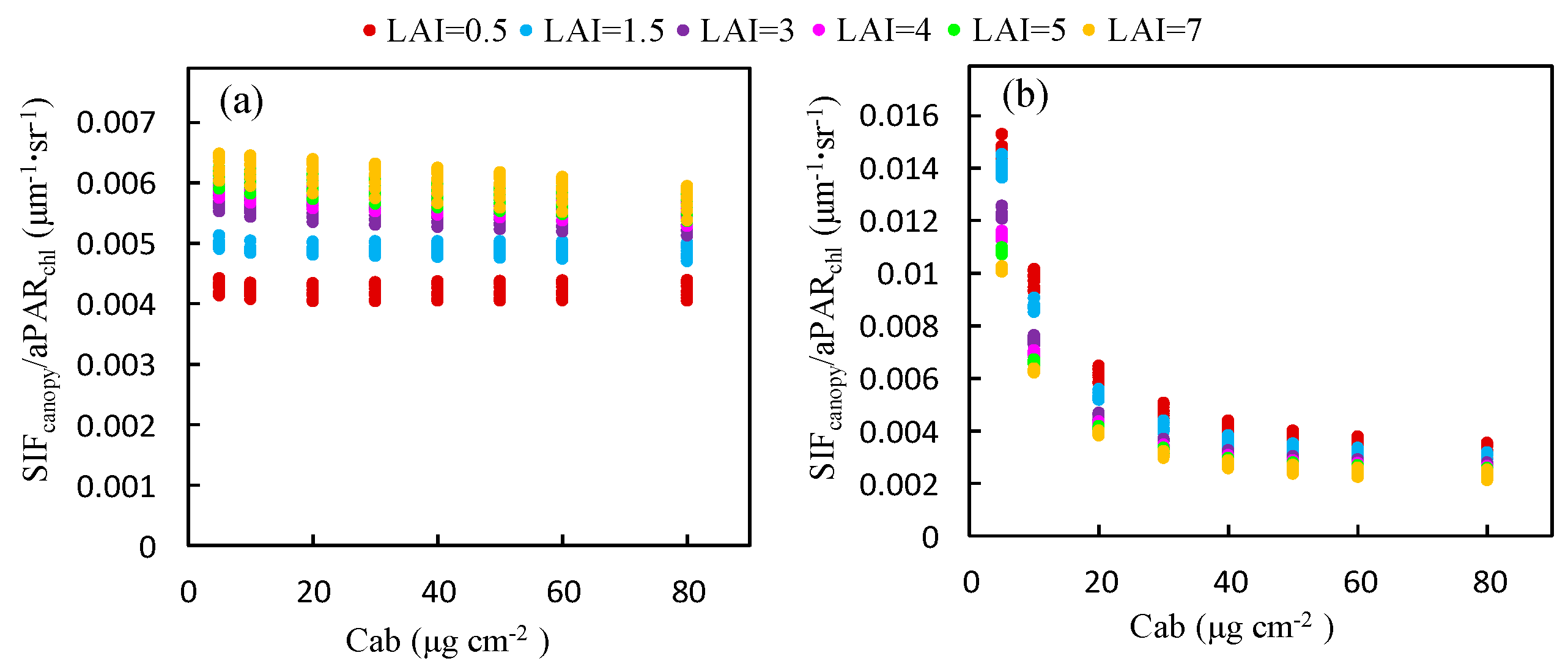
The ratio of to for different Cab levels was also calculated using the simulated dataset, as illustrated in Figure 5, which represents the response of to . The ratio of to is equal to the product of the fluorescence efficiency () and the fraction of SIF photons escaping the canopy (). was fixed in the simulation experiment and hence, in this experiment, this ratio was determined by . At the O2-B band, decreases markedly from 0.016 to 0.002 μm−1 sr−1 as Cab increases but, at the O2-A band, it remains almost constant for a given LAI. Therefore, the ratio of to is less influenced by the Cab content at the O2-A band than the O2-B band, which accounts for the linear relationship between and at the O2-A band, which exists no matter what the value of Cab is.
3.2.2. Effect of LAI on the Relationship between and
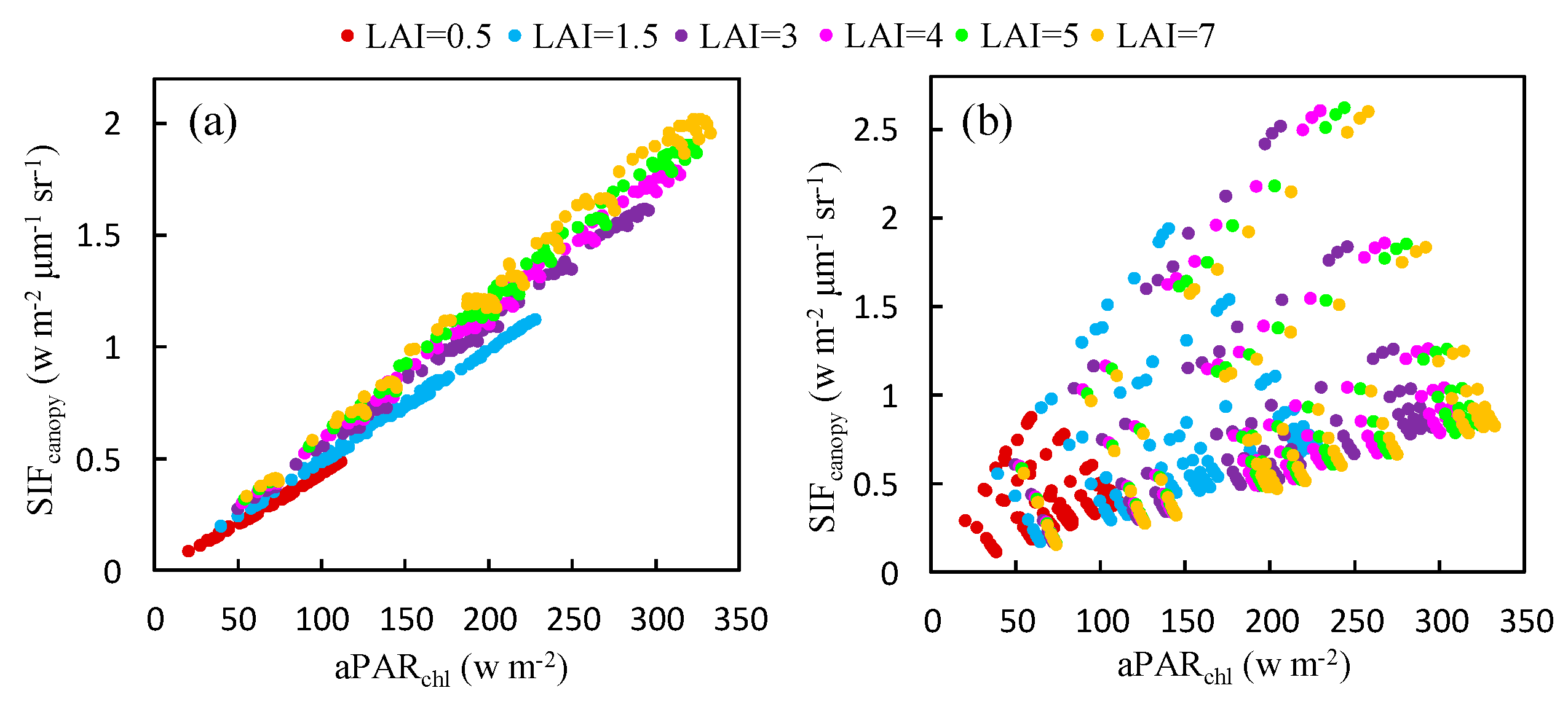
Using the simulated dataset, the response of to at both bands was also investigated for canopies with different values of the LAI (see Figure 6). It can be seen that, at the O2-A band, this relationship varies very little as the LAI changes, especially for dense vegetation (LAI > 3). However, for the O2-B band, plotting the relationship between and produces a very scattered distribution (Figure 6b) because it is dominated by Cab as illustrated in Figure 5b.
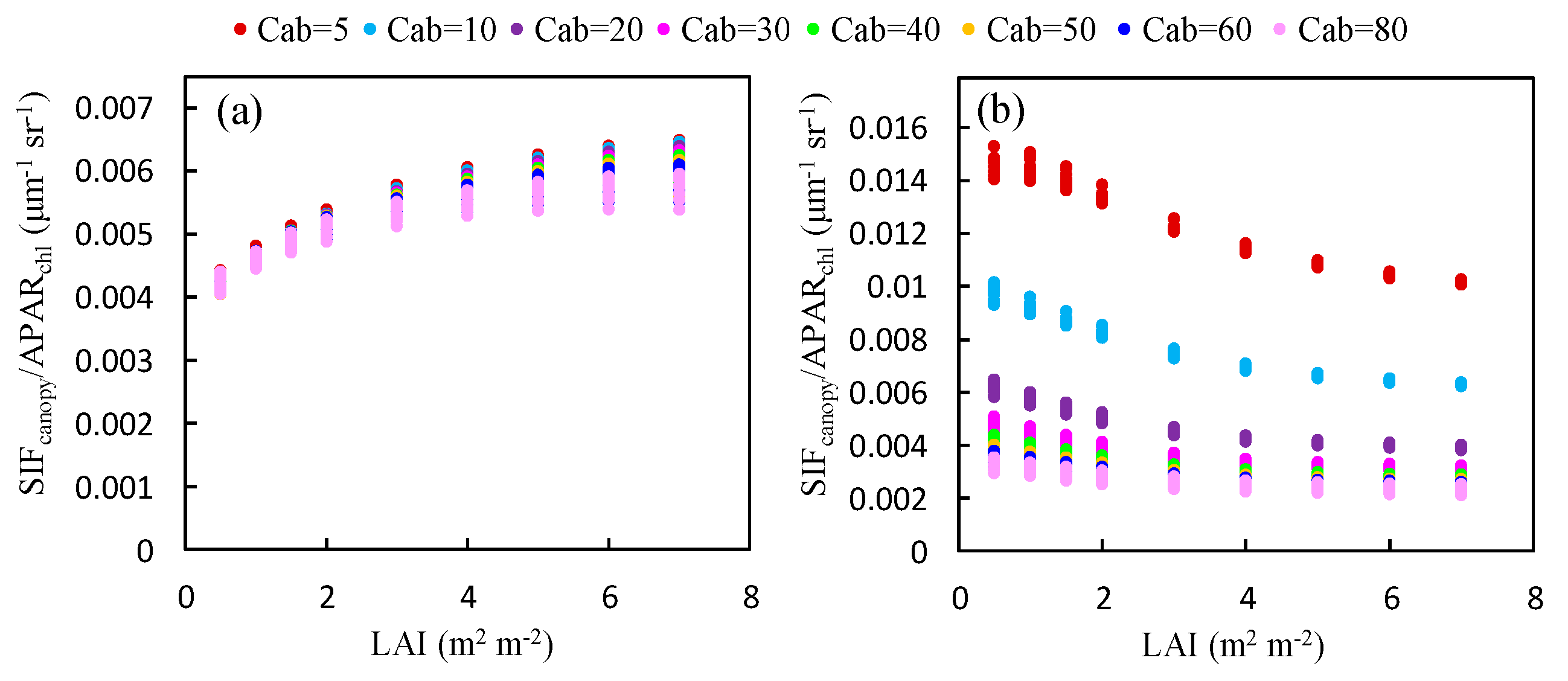
The ratio of to at the O2-A band increases with LAI (Figure 7a). An opposite trend is observed at the O2-B band (Figure 7b). Except for the low Cab condition at the O2-B band, the ratio of to at both bands is almost saturated for values of the LAI greater than 3 and the influence of the LAI decreases as Cab increases. This can be contributed to the effects of reabsorption and scattering at different wavelengths. At the O2-B band, the reflectance is very low (<5%) and the reabsorption effect of increases with larger LAI values; therefore, the ratio of to decreases with increased LAI. At the O2-A band, the leaf reflectance and transmittance is high (40–60%) and the reabsorption effect due to can be neglected. Therefore, the increases with larger LAI and is determined by the scattering mechanism at the near infrared (NIR) band.
3.2.3. Effect of Plant Structure Type on the Relationship between and
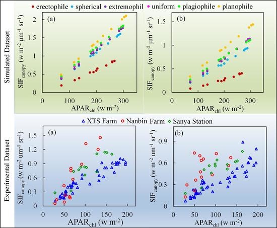
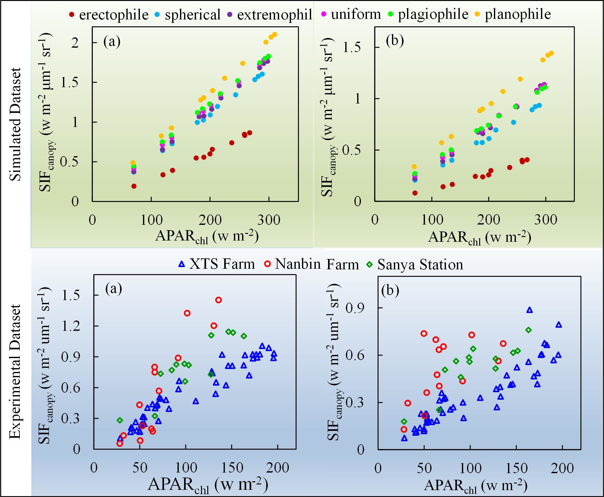
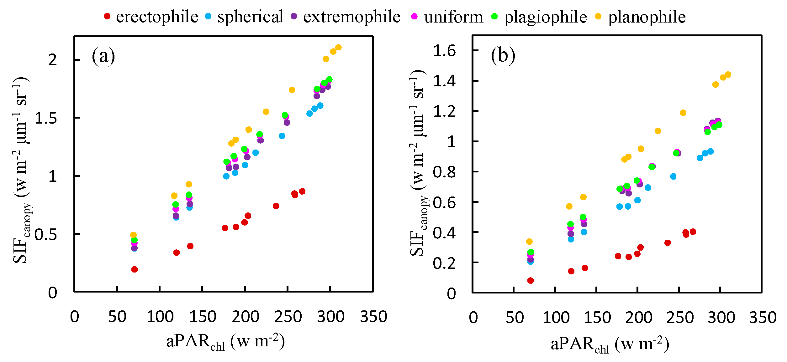
To explore whether the relationship between and depends on the plant type, a simulation using different leaf angle distribution functions was carried out to investigate the relationship between and at both the O2-A and O2-B bands. The results are illustrated in Figure 8. Six plant types, described in terms of different values of LIDFa and LIDFb, were used in the simulation. LIDFa determines the leaf inclination whereas LIDFb describes the variation in leaf inclination. At the O2-A band, the slopes for the relationships shown in Figure 8 range from 0.0035 μm−1 sr−1 for erectophile-type plants to 0.0067 μm−1 sr−1 for planophile-type plants. Similarly, for the O2-B band, the slope values are 0.0017 μm−1 sr−1 and 0.0046 μm−1 sr−1 for erectophile-type plants and planophile-type plants, respectively. This means that the fraction of re-emitted by chlorophyll fluorescence and observed at the top of the canopy is higher for planophile-type plants than erectophile-type plants when the same amount of PAR is absorbed by chlorophyll. For planophile plants, the fraction of fluorescence photons that escape from the lower leaves is much lower than from the top leaves. Therefore, the increase in the slope of against as the LAD (leaf angle distribution) becomes more horizontal can be considered due to the different PAR distribution within canopies with different canopy structures.
The slope of to was also calculated for different plant types. For a given plant type, remains almost constant when LAI and Cab are constant. However, for planophile plants, the slope is 3.51 times higher than for erectophile plants at the O2-B band and 2.26 times higher at the O2-A band. The results illustrated in Figure 8 indicates, therefore, that the GPP- relationship may be species-specific.
3.3. The Relationship between and Based on the Experimental Data
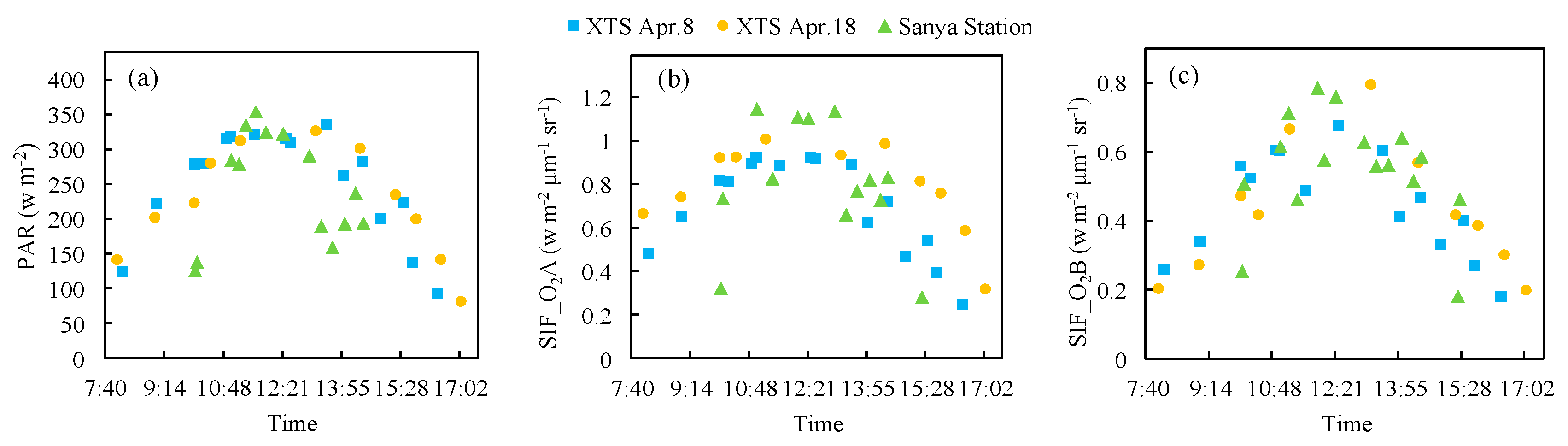
3.3.1. The Diurnal Cycle of Incoming PAR and SIF Signal for XTSApr and Sanya Station
Figure 9 illustrates the diurnal observations of incoming PAR and SIF at O2-A and O2-B bands of the diurnal experiments at XTS Farm in April and Sanya Station. As shown in Figure 9, the diurnal variation in the SIF signal at O2-A and O2-B bands are similar to that for the incoming PAR, and the emitted SIF is synchronously responded to the incoming PAR.
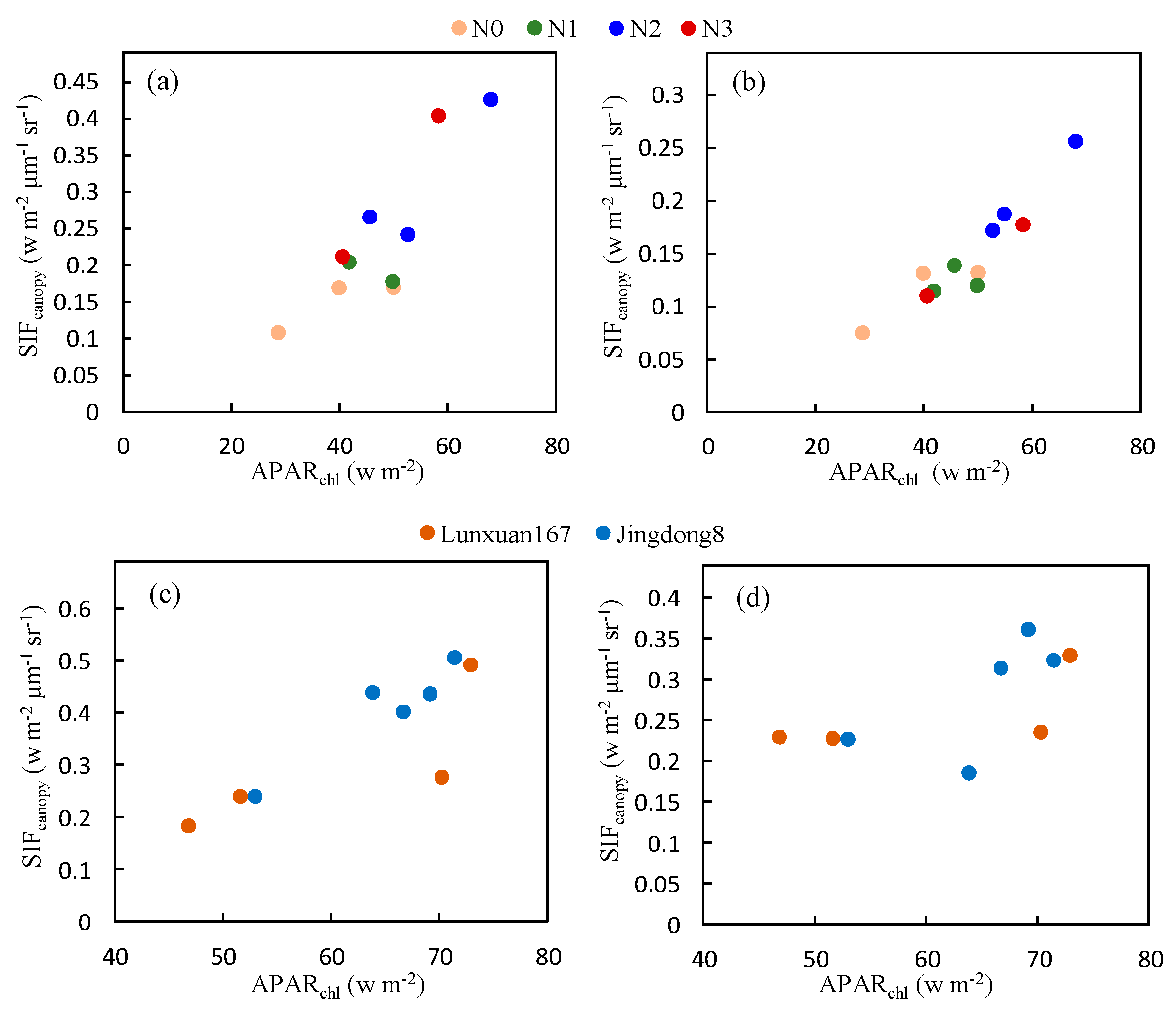
3.3.2. The Influence of Different Fertilization Treatments and Varieties on the Relationship between and
The effect of different fertilization treatments and varieties on the relationship between and was shown in Figure 10. There was no obvious effect of fertilization treatment on the slope of the relationship so the fertilization treatment only influenced the growth status, which only showed a higher and with the most appropriate fertilization treatment (N2). We can also conclude that the discrepancy of this relationship between different varieties was negligible.
3.3.3. Effect of Cab and on the Relationship between and
As illustrated in Figure 11, the relationship between at O2-A band and is not significantly affected by Cab content based on the experimental measurements conducted on Nanbin and XTS Farm. However, for the O2-B band, the plots are more diverse if Cab varies greatly as shown in Figure 11a,b for observations at Nanbin Farm. The diurnal experiments were conducted during two periods in April 2016 at XTS Farm, and the Cab content of the wheat leaves at each period varied little during the period of the experiments, with a Cab value of 55.29 and 53.62 μg/cm2. So, the relationship was linear at the O2-B band.
The effect of on the relationship between at both bands and was also analyzed using the experimental measurements (see Figure 12). Similar to the effect of the Cab content, the response of at the O2-A band to was linear under different conditions. But at the O2-B band, the relationship varies as the changes for Nanbin Farm.
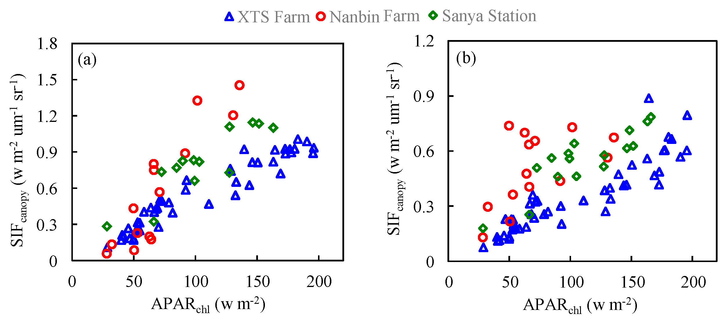
3.3.4. Effect of Plant Structure Type on the Relationship between and
Figure 13 shows scatter plots of against at the O2-A and O2-B bands based on all the experimental data. Compared to the simulated data, the measured patterns show a more diverse distribution while also presenting approximate linear relationships for experiments at different sites. It clearly shows that the slope of to is higher for experimental observations with planophile canopy structure at Nanbin Farm and Sanya Station than that for winter wheat with spherical canopy structure at XTS Farm.
4. Discussion
4.1. Uncertainties in the SIF Retrieval and Measurements
The SIF retrieval accuracy is dependent on the spectral characteristics of the sensor, such as the SR (spectral resolution) and SNR (signal-to-noise ratio). In this paper, the spectral data was acquired by a QE Pro spectrometer with an SR of 0.3 nm and a peak SNR >1000. According to the work by Liu et al. [16], using the 3FLD method, the SIF retrieval error should be less than 15%. Therefore, because of the high SR and SNR of the QE Pro spectrometer, it is reasonable to believe that the accuracy of the retrieved SIF is good and, hence, that the results describing the ability of the to estimate the described here are reliable. The significant correlation between and indicates that the SIF may be a better proxy for estimation.
The studies by Fournier et al. [44] and Damn et al. [45] showed that, due to variations in the direct and diffuse radiation and also the bi-directional reflectance distribution function (BRDF) characteristics of the canopy, the illumination conditions also have an influence on the retrieval of SIF. The different absorption depths at the oxygen absorption bands that absorb direct and diffuse radiation can lead to an overestimate or underestimate of the SIF at specific observation geometries. In this study, all the measurements of were carried out at nadir conditions. According to the simulations, the error in the SIF retrieval caused by the nonlinear mixing of direct and diffuse radiation is less than 5% for nadir observations under clear-sky conditions and a solar zenith angle larger than . It is, therefore, reasonable to neglect the influence of this nonlinear mixing of direct and diffuse radiation.
The method proposed by Liu et al. [43] was adopted to measure the. According to the validation carried out by Liu et al. [43], which was based on a comparison of fPAR measurements made by a digital camera and those made by a SunScan instrument (Delta-T, Inc., Cambridge, UK) in the 400–700 nm spectral range with a resolution of 0.30 μmol−1 m−2 s−1, there was a significant correlation between the two types of measurement—the mean absolute error was 0.031 and the mean relative error 6.037%. Therefore, the accuracy of fPAR measurements can be considered reliable. In the present study, the ratio of to was calculated using a simulated dataset with different values of Cab and LAI and a mean value of the ratio of to depending on different Cab content level was used. For example, if Cab was 5 and 10 μg cm−2, the ratio used the simulated value. The range of this ratio was 0.775–0.81 for Cab greater than 20 μg cm−2 and so the uncertainty in the calculation of and should have been smaller than 3%.
4.2. The Link between and
In this study, we investigated the relationship between and using both simulated and field-measured datasets. is a key parameter linking SIF to GPP and so the results of this study may serve as a reference for the estimation of GPP using SIF. It is an important issue in studies of applications using SIF and it is still a matter of debate [46,47]. According to Porcar-Castell et al. [29], the emitted SIF contains contributions from both photosystem I (PS I) and photosystem II (PS II). Compared to the SIF in the far-red part of the spectrum, the SIF in the red band is more closely linked to the activity of PS II. The SIF yield of PS II is considered to be more sensitive to variations in illumination and physiological or biochemical parameters [30,48]. Therefore, at the photosystem level, it is reasonable to believe that the SIF in the red part of the spectrum is more closely related to the GPP. However, in remote sensing applications at the canopy level, only the SIF signal that escapes from the canopy can be detected; the SIF is reabsorbed by chloroplasts during the radiative transfer process within the leaves and canopy [49,50,51,52] and so the characteristics of are different to those of .
In this study, the simulated data showed that the relationship between at O2-A band and is relatively insensitive to the LAI and Cab content compared to the O2-B band and can be expressed by a unique linear relationship at the O2-A band. However, at the O2-B band, this relationship is significantly influenced by the LAI and Cab content. The effect of the Cab content on the ratio of to is larger than that due to the LAI. This can be interpreted as meaning that the fluorescence photons emitted at the photosystem level can be reabsorbed by chlorophyll within the leaf or during the radiative transfer process from the leaf to the canopy. This reabsorption occurs because the fluorescence emission spectrum overlaps the chlorophyll absorption spectrum [30]. The absorption of chlorophyll at the red band is much stronger than that at the far-red band and the rate of reabsorption of red fluorescence can reach 90% [53]. As a result, at the O2-B band is strongly influenced by pigments and the correlation between and here is more sensitive to the Cab content than at the O2-A band.
As Porcar-Castell et al. [30] stated, at the red band, reabsorption effects dominate the amount of fluorescence escaping from the canopy. As verified by both simulations and field experiments, the ratio of to at both the O2-A and O2-B bands varies with the leaf angle distribution function, with more horizontal canopies having a larger ratio of to . This indicates that the large uncertainty in can weaken the relationship between the remotely sensed red SIF and or GPP.
4.3. The Consistency between Simulations and Experimental Measurements
Figure 8 and Figure 13 illustrate the scatter plots of and for both O2-A and O2-B bands based on the simulated dataset and experimental dataset, respectively. The results clearly show that the regression relationship between and is significantly different due to different canopy structures, which results in the discrepancies of the values of the ratio of to . Furthermore, both simulated dataset and experimental measurements indicate that the ratio of to increases when canopy structure becomes more horizontal. The corresponding statistical models are listed in Table 3. As illustrated in Table 3, at the O2-A band, for the linear regression models that have an offset of 0, the ratios of to with confidence level of 95% are 0.0092, 0.0076 and 0.0052 μm−1 sr−1 at the O2-A band and 0.0063 , 0.0049 and 0.0033 μm−1 sr−1 at the O2-B band for the Nanbin Farm, Sanya Station and XTS Farm experiments, respectively. The slopes derived from the observations correspond well with the simulations, which give values of 0.0055 and 0.0068 μm−1 sr−1 at the O2-A band and 0.0032 and 0.0047 μm−1 sr−1 at the O2-B band for spherical and planophile canopies, respectively. Especially, the ratios of to are almost the same for simulations and observations at the O2-B band. Thus, this further indicates that the ratio of to is dependent on the canopy structure.
Although the ratios of to derived from the simulations agree with those from the field measurements, there is still a small discrepancy between the two datasets. In the simulations by the SCOPE model, only Cab, LAI, SZA and the leaf inclination distribution type were considered, which does not correspond to the much more complicated natural conditions. For example, the fluorescence quantum yield, , was set to 0.01 [54]. However, the fluorescence quantum yield depends on the light intensity and other environmental conditions [14,28,35]. Therefore, although the effect of the radiative transfer mechanism within the canopy on the relationship between and was explored in this paper, the effect of the physiological mechanism remains unclear and will be a challenge for future studies.
5. Conclusions
In this study, we explored the response of to for both the O2-A and O2-B bands using both a simulation carried out by the SCOPE model and also field observations. The results showed that, at both these bands, had a strong linear relationship with for a canopy with a constant LAI and Cab content.
At the O2-A band, compared to the O2-B band, the relationship between and is relatively insensitive to the LAI and Cab content based on the simulated dataset, which are primarily determined by the specific vegetation structure. In contrast, the response of to at the O2-B band is very sensitive to the LAI and Cab content even for canopies with the same structure (the same LAD in the simulation experiment). This confirms that, at the O2-B band, due to reabsorption effects, is more influenced by the biochemical components of the canopy. The ratio of to was also analyzed for different concentrations of biochemical components and canopy structures and it was found that the influence of these factors is greater at the O2-B band than it at the O2-A band. As Cab increases, the ratio of to ranges from 0.016 to 0.002 μm−1 sr−1 for the O2-B band but remains almost invariant at the O2-A band for a given LAI. Similarly, based on the field experiments, the effect of different fertilization treatments and varieties on the relationship between and is negligible. The relationship between and is also not significantly affected by Cab content and at O2-A band compared to O2-B band.
The effect of LAD on the relationship between and was also investigated using both simulations and field observations. The relationship between and varies for different LAD functions and the slope of the graph of against decreases for a more erect canopy. The ratio of to is also different for different LAD functions with the highest ratio being for planophile plants and the lowest value for erectophile plants. For a given LAI and Cab content, the ratio ranges from 0.0068 μm−1 sr−1 for planophile plants to 0.0031 μm−1 sr−1 for erectophile plants at the O2-A band and from 0.0047 to 0.0014 μm−1 sr−1 for both types of plant at the O2-B band. Similarly, based on the field observations, at the O2-A band, the ratios are 0.0076 and 0.0052 μm−1 sr−1 for gold coin grass with plain leaves and winter wheat with spherical leaves, respectively; the corresponding values at the O2-B band are 0.0049 and 0.0033 μm−1 sr−1, which corresponds well to the simulated results. These results show that the relationship between and varies according to the plant type, which agrees with the dependence of on GPP for specific plant types. However, the influence of the physiological structure of vegetation on the correlation between and GPP awaits more detailed investigation in future studies.
Therefore, the results of this study clearly show that there is a linear relationship between and , but that this relationship varies with the canopy biochemical components and canopy structure. The results also show that the reabsorption and scattering effects that occur during the radiative transfer from the photosystem to the canopy level should be corrected for before the remotely sensed is linked to the GPP.
Acknowledgments
The authors gratefully acknowledge the financial support provided by the National Key Research and Development Program of China (2017YFA0603001), and the National Natural Science Foundation of China (41671349).
Author Contributions
Shanshan Du and Liangyun Liu conceived and designed the research. Shanshan Du conducted the experiments and data analysis, and prepared the manuscript. Liangyun Liu contributed significantly to the research method and the manuscript revision. Xinjie Liu and Jiaochan Hu made important contributions to the field experiments.
Conflicts of Interest
The authors declare no conflict of interest.
References
- Beer, C.; Reichstein, M.; Tomelleri, E.; Ciais, P.; Jung, M.; Carvalhais, N.; Rödenbeck, C.; Arain, M.A.; Baldocchi, D.; Bonan, G.B. Terrestrial gross carbon dioxide uptake: Global distribution and covariation with climate. Science 2010, 329, 834–838. [Google Scholar] [CrossRef] [PubMed]
- Yu, G.R.; Zhu, X.J.; Fu, Y.L.; He, H.L.; Wang, Q.F.; Wen, X.F.; Li, X.R.; Zhang, L.M.; Zhang, L.; Su, W. Spatial patterns and climate drivers of carbon fluxes in terrestrial ecosystems of China. Glob. Chang. Biol. 2013, 19, 798–810. [Google Scholar] [CrossRef] [PubMed]
- Baldocchi, D. Measuring fluxes of trace gases and energy between ecosystems and the atmosphere–the state and future of the eddy covariance method. Glob. Chang. Biol. 2014, 20, 3600–3609. [Google Scholar] [CrossRef] [PubMed]
- Jung, M.; Reichstein, M.; Margolis, H.A.; Cescatti, A.; Richardson, A.D.; Arain, M.A.; Arneth, A.; Bernhofer, C.; Bonal, D.; Chen, J. Global patterns of land-atmosphere fluxes of carbon dioxide, latent heat, and sensible heat derived from eddy covariance, satellite, and meteorological observations. J. Geophys. Res. 2011, 116, 245–255. [Google Scholar] [CrossRef]
- Xiao, J.F.; Zhuang, Q.L.; Law, B.E.; Chen, J.; Baldocchi, D.D.; Cook, D.R.; Oren, R.; Richardson, A.D.; Wharton, S.; Ma, S. A continuous measure of gross primary production for the conterminous United States derived from MODIS and AmeriFlux data. Remote Sens. Environ. 2009, 114, 576–591. [Google Scholar] [CrossRef]
- Xiao, J.; Ollinger, S.V.; Frolking, S.; Hurtt, G.C.; Hollinger, D.Y.; Davis, K.J.; Pan, Y.; Zhang, X.; Deng, F.; Chen, J. Data-driven diagnostics of terrestrial carbon dynamics over North America. Agric. For. Meteorol. 2014, 197, 142–157. [Google Scholar] [CrossRef]
- Zeng, N.; Mariotti, A.; Wetzel, P. Terrestrial mechanisms of interannual CO2 variability. Glob. Biogeochem. Cycles 2005, 19, 159–171. [Google Scholar] [CrossRef]
- Collatz, G.J.; Ribascarbo, M.; Berry, J.A. Coupled photosynthesis-stomatal conductance model for leaves of C4 plants. Funct. Plant Biol. 1992, 19, 519–538. [Google Scholar]
- Xia, J.; Chen, J.; Piao, S.; Ciais, P.; Luo, Y.; Wan, S. Terrestrial carbon cycle affected by non-uniform climate warming. Nat. Geosci. 2014, 7, 173–180. [Google Scholar] [CrossRef]
- Running, S.W.; Nemani, R.R.; Heinsch, F.A.; Zhao, M.S.; Reeves, M.; Hashimoto, H. A continuous satellite-derived measure of global terrestrial primary production. BioScience 2004, 54, 547–560. [Google Scholar] [CrossRef]
- Yuan, W.P.; Liu, S.G.; Zhou, G.S.; Zhou, G.Y.; Tieszen, L.L.; Baldocchi, D.; Bernhofer, C.; Gholz, H.; Goldstein, A.H.; Goulden, M.L. Deriving a light use efficiency model from eddy covariance flux data for predicting daily gross primary production across biomes. Agric. For. Meteorol. 2007, 143, 189–207. [Google Scholar] [CrossRef]
- Xiao, X.; Hollinger, D.; Aber, J.; Goltz, M.; Davidson, E.A.; Zhang, Q.; Iii, B.M. Satellite-based modeling of gross primary production in an evergreen needleleaf forest. Remote Sens. Environ. 2004, 89, 519–534. [Google Scholar] [CrossRef]
- Xiao, X.; Zhang, Q.; Braswell, B.; Urbanski, S.; Boles, S.; Wofsy, S.; Iii, B.M.; Ojima, D. Modeling gross primary production of temperate deciduous broadleaf forest using satellite images and climate data. Remote Sens. Environ. 2004, 91, 256–270. [Google Scholar] [CrossRef]
- Berry, J.A.; Frankenberg, C.; Wennberg, P.O. A new method for measurement of photosynthesis from space. In Proceedings of the AGU Fall Meeting, San Francisco, CA, USA, 9–13 December 2013. [Google Scholar]
- Damm, A.; Guanter, L.; Paul-Limoges, E.; van der Tol, C.; Hueni, A.; Buchmann, N.; Eugster, W.; Ammann, C.; Schaepman, M.E. Far-red sun-induced chlorophyll fluorescence shows ecosystem-specific relationships to gross primary production: An assessment based on observational and modeling approaches. Remote Sens. Environ. 2015, 166, 91–105. [Google Scholar] [CrossRef]
- Liu, L.; Liu, X.; Hu, J. Effects of spectral resolution and SNR on the vegetation solar-induced fluorescence retrieval using FLD-based methods at canopy level. Eur. J. Remote Sens. 2015, 48, 743–762. [Google Scholar] [CrossRef]
- Rascher, U.; Alonso, L.; Burkart, A.; Cilia, C.; Cogliati, S.; Colombo, R.; Damm, A.; Drusch, M.; Guanter, L.; Hanus, J. Sun-induced fluorescence—A new probe of photosynthesis: First maps from the imaging spectrometer HyPlant. Glob. Chang. Biol. 2015, 21, 4673–4684. [Google Scholar] [CrossRef] [PubMed] [Green Version]
- Joiner, J.; Yoshida, Y.; Vasilkov, A.P.; Corp, L.A.; Middleton, E.M. First observations of global and seasonal terrestrial chlorophyll fluorescence from space. Biogeosci. Discuss. 2011, 8, 637–651. [Google Scholar] [CrossRef] [Green Version]
- Frankenberg, C.; Fisher, J.B.; Worden, J.; Badgley, G.; Saatchi, S.S.; Lee, J.E.; Toon, G.C.; Butz, A.; Jung, M.; Kuze, A. New global observations of the terrestrial carbon cycle from GOSAT: Patterns of plant fluorescence with gross primary productivity. Geophys. Res. Lett. 2011, 38, 351–365. [Google Scholar] [CrossRef]
- Köhler, P.; Guanter, L.; Frankenberg, C. Simplified physically based retrieval of sun-induced chlorophyll fluorescence from GOSAT data. IEEE Geosci. Remote Sens. Lett. 2015, 12, 1446–1450. [Google Scholar] [CrossRef]
- Guanter, L.; Frankenberg, C.; Dudhia, A.; Lewis, P.E.; Gómez-Dans, J.; Kuze, A.; Suto, H.; Grainger, R.G. Retrieval and global assessment of terrestrial chlorophyll fluorescence from GOSAT space measurements. Remote Sens. Environ. 2012, 121, 236–251. [Google Scholar] [CrossRef]
- Frankenberg, C.; O′Dell, C.; Berry, J.; Guanter, L.; Joiner, J.; Köhler, P.; Pollock, R.; Taylor, T.E. Prospects for chlorophyll fluorescence remote sensing from the Orbiting Carbon Observatory-2. Remote Sens. Environ. 2014, 147, 1–12. [Google Scholar] [CrossRef]
- Joiner, J.; Yoshida, Y.; Vasilkov, A.P.; Middleton, E.M.; Campbell, P.K.E.; Yoshida, Y.; Kuze, A.; Corp, L.A. Filling-in of near-infrared solar lines by terrestrial fluorescence and other geophysical effects: Simulations and space-based observations from SCIAMACHY and GOSAT. Atmos. Meas. Tech. 2012, 5, 163–210. [Google Scholar] [CrossRef]
- Joiner, J.; Yoshida, Y.; Guanter, L.; Middleton, E.M. New methods for retrieval of chlorophyll red fluorescence from hyper-spectral satellite instruments: Simulations and application to GOME-2 and SCIAMACHY. Atmos. Meas. Tech. 2016, 9, 3939–3967. [Google Scholar] [CrossRef]
- Joiner, J.; Guanter, L.; Lindstrot, R.; Voigt, M.; Vasilkov, A.P.; Middleton, E.M.; Huemmrich, K.F.; Yoshida, Y.; Frankenberg, C. Global monitoring of terrestrial chlorophyll fluorescence from moderate spectral resolution near-infrared satellite measurements: Methodology, simulations, and application to GOME-2. Atmos. Meas. Tech. 2013, 6, 2803–2823. [Google Scholar] [CrossRef]
- Köhler, P.; Guanter, L.; Joiner, J. A linear method for the retrieval of sun-induced chlorophyll fluorescence from GOME-2 and SCIAMACHY data. Atmos. Meas. Tech. 2015, 8, 2589–2608. [Google Scholar] [CrossRef]
- Zhao, M.; Running, S.; Heinsch, F.A.; Nemani, R. MODIS-derived terrestrial primary production. In Land Remote Sensing and Global Environmental Change; Springer: New York, NY, USA, 2010; pp. 635–660. [Google Scholar]
- Huete, A.; Ponce-Campos, G.; Zhang, Y.; Restrepo-Coupe, N.; Ma, X.; Moran, M.S. Monitoring Photosynthesis from Space. In Land Resources Monitoring, Modeling, and Mapping with Remote Sensing; CRC Press: Boca Raton, FL, USA, 2015; pp. 3–22. [Google Scholar]
- Liu, L.; Liu, X.; Wang, Z. Measurement and analysis of bidirectional SIF emissions in wheat canopies. IEEE Trans. Geosci. Remote Sens. 2016, 54, 2640–2651. [Google Scholar] [CrossRef]
- Porcar-Castell, A.; Tyystjärvi, E.; Atherton, J.; van der Tol, C.; Flexas, J.; Pfündel, E.E.; Moreno, J.; Frankenberg, C.; Berry, J.A. Linking chlorophyll a fluorescence to photosynthesis for remote sensing applications: Mechanisms and challenges. J. Exp. Bot. 2014, 65, 4065. [Google Scholar] [CrossRef] [PubMed]
- Guanter, L.; Zhang, Y.; Jung, M.; Joiner, J.; Voigt, M.; Berry, J.A.; Frankenberg, C.; Huete, A.R.; Zarco-Tejada, P.; Lee, J.E. Reply to Magnani et al.: Linking large-scale chlorophyll fluorescence, observations with cropland gross primary production. Proc. Natl. Acad. Sci. USA 2014, 111, E2511. [Google Scholar] [CrossRef] [PubMed]
- Wang, Z. Sunlit Leaf Photosynthesis Rate Correlates Best with Chlorophyll Fluorescence of Terrestrial Ecosystems. Master’s Thesis, University of Toronto, Toronto, ON, Canada, 2014. [Google Scholar]
- Zhang, Y.; Guanter, L.; Berry, J.A.; Tol, C.V.D.; Yang, X.; Tang, J.; Zhang, F. Model-based analysis of the relationship between sun-induced chlorophyll fluorescence and gross primary production for remote sensing applications. Remote Sens. Environ. 2016, 187, 145–155. [Google Scholar] [CrossRef]
- Liu, L.; Guan, L.; Liu, X. Directly estimating diurnal changes in GPP for C3 and C4 crops using far-red sun-induced chlorophyll fluorescence. Agric. For. Meteorol. 2017, 232, 1–9. [Google Scholar] [CrossRef]
- Schlau-Cohen, G.S.; Berry, J. Photosynthetic fluorescence, from molecule to planet. Phys. Today 2015, 68, 66–67. [Google Scholar] [CrossRef]
- Yang, X.; Tang, J.; Mustard, J.F.; Lee, J.-E.; Rossini, M.; Joiner, J.; Munger, J.W.; Kornfeld, A.; Richardson, A.D. Solar-induced chlorophyll fluorescence that correlates with canopy photosynthesis on diurnal and seasonal scales in a temperate deciduous forest. Geophys. Res. Lett. 2015, 42, 2977–2987. [Google Scholar] [CrossRef]
- Lee, J.E.; Berry, J.A.; Christiaan, V.D.T.; Yang, X.; Guanter, L.; Damm, A.; Baker, I.; Frankenberg, C. Simulations of chlorophyll fluorescence incorporated into the Community Land Model version 4. Glob. Chang. Biol. 2015, 21, 3469. [Google Scholar] [CrossRef] [PubMed] [Green Version]
- Van der Tol, C.; Verhoef, W.; Rosema, A. A model for chlorophyll fluorescence and photosynthesis at leaf scale. Agric. For. Meteorol. 2009, 149, 96–105. [Google Scholar] [CrossRef]
- Plascyk, J.A.; Ribas-Carbo, M.; Berry, J. The MK II Fraunhofer Line Discriminator (FLD-II) for airborne and orbital remote sensing of solar-stimulated luminescence. Opt. Eng. 1975, 14, 339–346. [Google Scholar] [CrossRef]
- Maier, S.W.; Günther, K.P.; Stellmes, M. Sun-induced fluorescence: A new tool for precision farming. In Digital Imaging and Spectral Techniques: Applications to Precision Agriculture and Crop Physiology; ASA Special Publication: Madison, WI, USA, 2003; pp. 209–222. [Google Scholar]
- Alonso, L.; Gómezchova, L.; Vilafrancés, J.; Amoros-Lopez, J.; Guanter, L.; Calpe, J.; Moreno, J. Improved Fraunhofer line discrimination method for vegetation fluorescence quantification. IEEE Geosci. Remote Sens. Lett. 2008, 5, 620–624. [Google Scholar] [CrossRef]
- Liu, L.; Liu, X.; Hu, J.; Guan, L. Assessing the wavelength-dependent ability of solar-induced chlorophyll fluorescence to estimate the GPP of winter wheat at the canopy level. Int. J. Remote Sens. 2017, 38, 4396–4417. [Google Scholar] [CrossRef]
- Liu, L.; Peng, D.; Hu, Y.; Jiao, Q. A novel in situ FPAR measurement method for low canopy vegetation based on a digital camera and reference panel. Remote Sens. 2013, 5, 274–281. [Google Scholar] [CrossRef]
- Fournier, A.; Goulas, Y.; Daumard, F.; Ounis, A.; Champagne, S.; Moya, I. Effects of vegetation directional reflectance on sun-induced fluorescence retrieval in the oxygen absorption bands. In Proceedings of the IEEE 5th International Workshop Remote Sensing of Vegetation Fluorescence, Paris, France, 22–24 April 2014; pp. 1–5. [Google Scholar]
- Damm, A.; Guanter, L.; Verhoef, W.; Schläpfer, D.; Garbari, S.; Schaepman, M.E. Impact of varying irradiance on vegetation indices and chlorophyll fluorescence derived from spectroscopy data. Remote Sens. Environ. 2015, 156, 202–215. [Google Scholar] [CrossRef]
- Verrelst, J.; Tol, C.V.D.; Magnani, F.; Sabater, N.; Rivera, J.P.; Mohammed, G.; Moreno, J. Evaluating the predictive power of sun-induced chlorophyll fluorescence to estimate net photosynthesis of vegetation canopies: A SCOPE modeling study. Remote Sens. Environ. 2016, 176, 139–151. [Google Scholar] [CrossRef]
- Goulas, Y.; Fournier, A.; Daumard, F.; Champagne, S.; Ounis, A.; Marloie, O.; Moya, I. Gross primary production of a wheat canopy relates stronger to far red than to red solar-induced chlorophyll fluorescence. Remote Sens. 2017, 9, 97. [Google Scholar] [CrossRef]
- Verrelst, J.; Rivera, J.P.; van der Tol, C.; Magnani, F.; Mohammed, G.; Moreno, J. Global sensitivity analysis of the SCOPE model: What drives simulated canopy-leaving sun-induced fluorescence? Remote Sens. Environ. 2015, 166, 8–21. [Google Scholar] [CrossRef]
- Yang, L. Structure of the red fluorescence band in chloroplasts. J. Gen. Phys. 1966, 49, 763–780. [Google Scholar]
- Brody, S.S.; Brody, M. Fluorescence properties of aggregated chlorophyll in vivo and in vitro. Trans. Faraday Soc. 1962, 58, 416–428. [Google Scholar] [CrossRef]
- Fournier, A.; Daumard, F.; Champagne, S.; Ounis, A.; Goulas, Y.; Moya, I. Effect of canopy structure on sun-induced chlorophyll fluorescence. ISPRS J. Photogramm. Remote Sens. 2012, 68, 112–120. [Google Scholar] [CrossRef]
- Middleton, E.M.; Cheng, Y.B.; Campbell, P.K.; Huemmrich, K.F.; Zhang, Q.; Kustas, W.P. Canopy level chlorophyll fluorescence and the PRI in a cornfield. In Proceedings of the IEEE International Geoscience and Remote Sensing Symposium (IGARSS) Munich, Germany, 22–27 July 2012; pp. 7117–7120. [Google Scholar]
- Gitelson, A.A.; Buschmann, C.; Lichtenthaler, H.K. Leaf chlorophyll fluorescence corrected for re-absorption by means of absorption and reflectance measurements. J. Plant Phys. 1998, 152, 283–296. [Google Scholar] [CrossRef]
- Van der Tol, C.; Berry, J.; Campbell, P.; Rascher, U. Models of fluorescence and photosynthesis for interpreting measurements of solar-induced chlorophyll fluorescence. J. Geophys. Res. 2014, 119, 2312–2327. [Google Scholar] [CrossRef] [PubMed] [Green Version]
Figure 1.
The distribution of the three experimental sites in China.
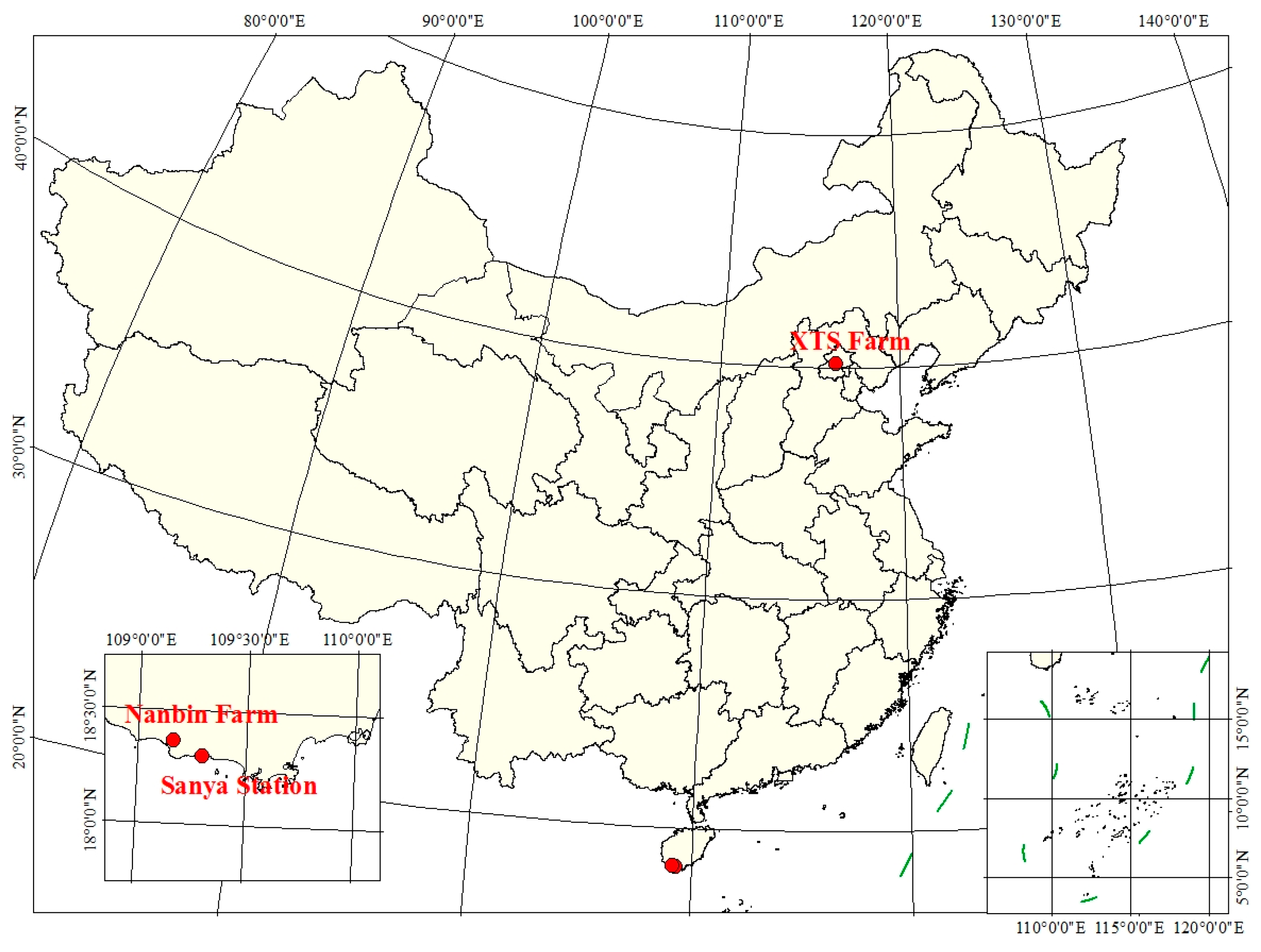
Figure 2.
The photographs of studied canopies at XTS Farm in November (left, winter wheat), Nanbin Farm (middle, cotton) and Sanya Station (right, gold coin grass).
Figure 2.
The photographs of studied canopies at XTS Farm in November (left, winter wheat), Nanbin Farm (middle, cotton) and Sanya Station (right, gold coin grass).
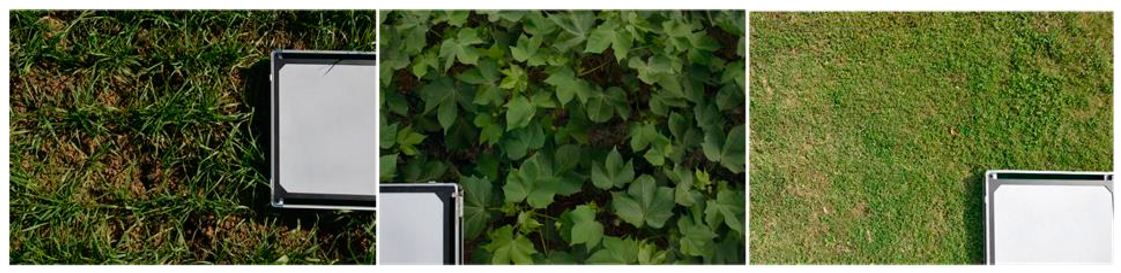
Figure 3.
The ratio of to for canopies with different LAI and Cab based on the simulation carried out by the SCOPE model.
Figure 3.
The ratio of to for canopies with different LAI and Cab based on the simulation carried out by the SCOPE model.

Figure 4.
The relationship between and APARchl at the O2-A (a) and O2-B (b) bands for different values of the Cab content. These results were obtained using the simulated dataset.
Figure 4.
The relationship between and APARchl at the O2-A (a) and O2-B (b) bands for different values of the Cab content. These results were obtained using the simulated dataset.

Figure 5.
The ratio of to for canopies with different Cab content at the O2-A (a) and O2-B (b) bands based on the simulated dataset.
Figure 5.
The ratio of to for canopies with different Cab content at the O2-A (a) and O2-B (b) bands based on the simulated dataset.

Figure 6.
The relationship between and at the O2-A (a) and O2-B (b) bands for different LAI values, as obtained using the simulated dataset.
Figure 6.
The relationship between and at the O2-A (a) and O2-B (b) bands for different LAI values, as obtained using the simulated dataset.

Figure 7.
The ratio of to for canopies with different values of the LAI at the O2-A (a) and O2-B (b) bands, as obtained using the simulated dataset.
Figure 7.
The ratio of to for canopies with different values of the LAI at the O2-A (a) and O2-B (b) bands, as obtained using the simulated dataset.

Figure 8.
The relationship between and at the O2-A (a) and O2-B (b) bands for different plant types, as obtained using the simulated dataset (LAI = 3 m2 m−2, Cab = 40 μg cm−2).
Figure 8.
The relationship between and at the O2-A (a) and O2-B (b) bands for different plant types, as obtained using the simulated dataset (LAI = 3 m2 m−2, Cab = 40 μg cm−2).

Figure 9.
The diurnal cycle of incoming PAR (a) and SIF (b,c) at O2-A and O2-B bands for XTSApr and Sanya Station measurements.
Figure 9.
The diurnal cycle of incoming PAR (a) and SIF (b,c) at O2-A and O2-B bands for XTSApr and Sanya Station measurements.

Figure 10.
The relationship between the and at the O2-A (a,c) and O2-B (b,d) bands for experiment data obtained under different fertilization treatments (a,b) and varieties (c,d) at XTS Farm in November.
Figure 10.
The relationship between the and at the O2-A (a,c) and O2-B (b,d) bands for experiment data obtained under different fertilization treatments (a,b) and varieties (c,d) at XTS Farm in November.

Figure 11.
The relationship between and at the O2-A (upper) and O2-B (bottom) bands for different values of the Cab content obtained using the experimental dataset at Nanbin (a) XTS (b,c) Farm.
Figure 11.
The relationship between and at the O2-A (upper) and O2-B (bottom) bands for different values of the Cab content obtained using the experimental dataset at Nanbin (a) XTS (b,c) Farm.
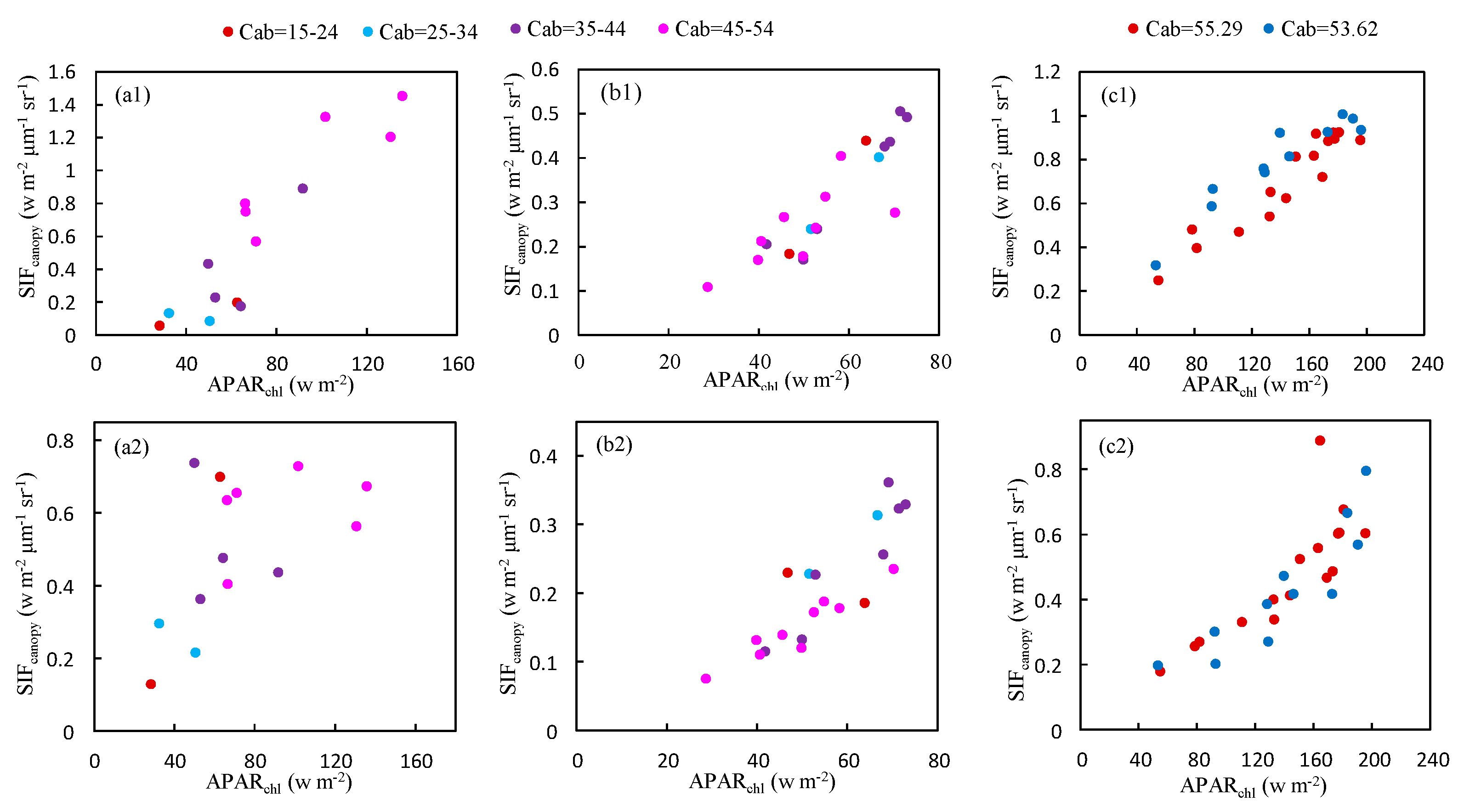
Figure 12.
The relationship between and at the O2-A (a,c) and O2-B (b,d) bands for different values of the obtained using the experimental dataset at Nanbin (a,b) and XTS (c,d) Farm in November.
Figure 12.
The relationship between and at the O2-A (a,c) and O2-B (b,d) bands for different values of the obtained using the experimental dataset at Nanbin (a,b) and XTS (c,d) Farm in November.
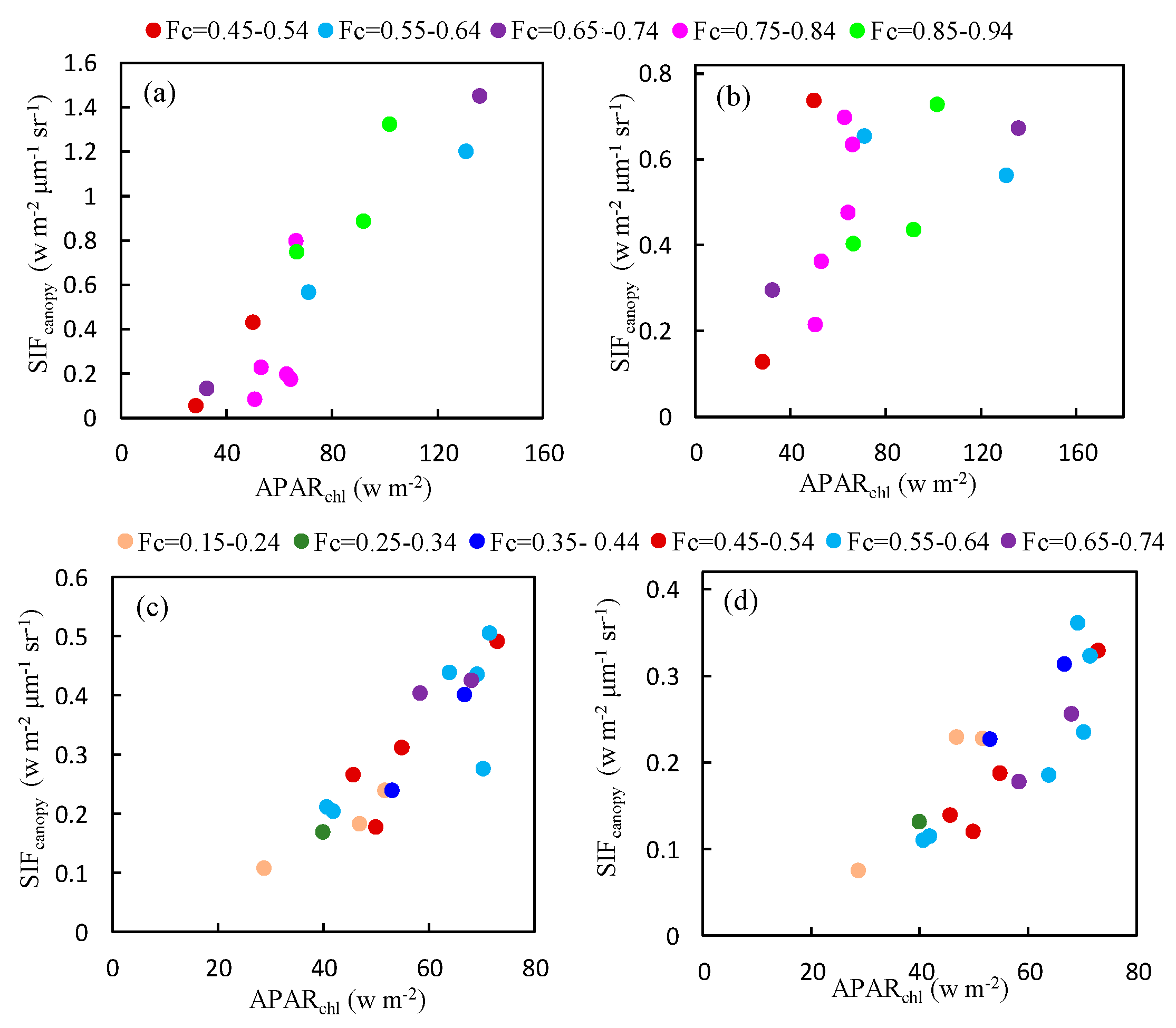
Figure 13.
The relationship between and at the O2-A (a) and O2-B (b) bands for different plant types based on the experimental data.
Figure 13.
The relationship between and at the O2-A (a) and O2-B (b) bands for different plant types based on the experimental data.


Table 1.
Main parameters of the SCOPE model used for the simulations in this study.
| Parameter | Description | Value/Range | Default | Unit |
|---|---|---|---|---|
| Cab | Leaf chlorophyll a + b content | 5, 10, 20, 30, 40, 50, 60, 80 | 40 | μg/cm2 |
| LAI | Leaf area index | 0.5, 1.5, 3, 4, 5, 7 | 3 | m2/m2 |
| LIDFa + LIDFb | Leaf inclination | [1, 0], [−1, 0], [0, −1], [0, 1], [0, 0], [−0.35, −0.15] | [−0.35, −0.15] | - |
| SZA | Solar zenith angle | 27, 29, 31, 36, 39, 46, 50, 57, 61, 68, 72 | - | degree |
| VZA | View zenith angle | 0 | - | degree |
[1, 0]—planophile; [−1, 0]—erectophile; [0, −1]—plagiophile; [0, 1]—extremophile; [0, 0]—uniform; [−0.35, −0.15]—spherical.
Table 2.
Details of the field experiments.
| XTSApr 8&9 Apr. | XTSApr 18 Apr. | XTSNov 7 Nov. | XTSNov 8 Dec. | Sanya Station | Nanbin Farm | |
|---|---|---|---|---|---|---|
| Latitude Longitude | 11′N 27′E | 11′N 27′E | 11′N 27′E | 11′N 27′E | 18′N 18′E | 22′N 10′E |
| Vegetation type | Wheat | Wheat | Wheat | Wheat | Gold coin grass | Vegetables and crops |
| Cab ( μg cm−2) | 55.29 | 53.68 | 40.98–54.38 | 21.22–54.38 | 40.83 | 15.22–56.68 |
| LAI (m2 m−2) | 2.48 | 2.92 | - | - | - | - |
| Canopy Structure | Spherical | Spherical | Spherical | Spherical | Planophile | Planophile |
| Fc | 0.72 | 0.79 | 0.15–0.52 | 0.21–0.63 | 0.67 | 0.28–0.91 |
| Objective | Diurnal experiment | Diurnal experiment | Fertilization treatments | Varieties treatments | Diurnal experiment | Multispecies experiment |
Table 3.
The statistical models linking and at the O2-A and O2-B bands derived using the experimental measurements and the simulated dataset.
Table 3.
The statistical models linking and at the O2-A and O2-B bands derived using the experimental measurements and the simulated dataset.
| Field Experiment Dataset | ||||||
| XTS Farm | Sanya Station | Nanbin Farm | All | |||
| O2-A band | y = 0.0050x + 0.0261 R2 = 0.9150, RMSE = 0.0820 y = 0.0052x () | y = 0.0065x + 0.1220 R2 = 0.7870, RMSE = 0.1540 y = 0.0076x () | y = 0.0134x − 0.3721 R2 = 0.8390, RMSE = 0.2030 y = 0.0092x () | y = 0.0062x + 0.0240 R2 = 0.6551, RMSE = 0.2070 y = 0.0064x | ||
| O2-B band | y = 0.0032x + 0.0095 R2 = 0.8190, RMSE = 0.0830 y = 0.0033x () | y = 0.0035x + 0.1650 R2 = 0.7070 RMSE = 0.0900 y = 0.0049x () | y = 0.0034x + 0.2559 R2 = 0.3360, RMSE = 0.1670 y = 0.0063x () | y = 0.0032x + 0.1103 R2 = 0.5192, RMSE = 0.1500 y = 0.0041x | ||
| Simulated Dataset | ||||||
| Erectophile | Spherical | Planophile | ||||
| O2-A band | y = 0.0035x − 0.0763 R2 = 0.9940, RMSE = 0.0170 y = 0.0031x () | y = 0.0057x − 0.0372 R2 = 0.9992, RMSE = 0.0120 y = 0.0055x () | y = 0.0067x + 0.0321 R2 = 0.9998, RMSE = 0.0160 y = 0.0068x () | |||
| O2-B band | y = 0.0017x − 0.0598 R2 = 0.979, RMSE = 0.0150 y = 0.0014x () | y = 0.0034x − 0.0506 R2 = 0.9965, RMSE = 0.014 y = 0.0032x () | y = 0.0046x + 0.0232 R2 = 0.9995, RMSE = 0.0090 y = 0.0047x () | |||
© 2017 by the authors. Licensee MDPI, Basel, Switzerland. This article is an open access article distributed under the terms and conditions of the Creative Commons Attribution (CC BY) license (http://creativecommons.org/licenses/by/4.0/).
Share and Cite
MDPI and ACS Style
Du, S.; Liu, L.; Liu, X.; Hu, J. Response of Canopy Solar-Induced Chlorophyll Fluorescence to the Absorbed Photosynthetically Active Radiation Absorbed by Chlorophyll. Remote Sens. 2017, 9, 911. https://doi.org/10.3390/rs9090911
AMA Style
Du S, Liu L, Liu X, Hu J. Response of Canopy Solar-Induced Chlorophyll Fluorescence to the Absorbed Photosynthetically Active Radiation Absorbed by Chlorophyll. Remote Sensing. 2017; 9(9):911. https://doi.org/10.3390/rs9090911
Chicago/Turabian StyleDu, Shanshan, Liangyun Liu, Xinjie Liu, and Jiaochan Hu. 2017. "Response of Canopy Solar-Induced Chlorophyll Fluorescence to the Absorbed Photosynthetically Active Radiation Absorbed by Chlorophyll" Remote Sensing 9, no. 9: 911. https://doi.org/10.3390/rs9090911
Note that from the first issue of 2016, this journal uses article numbers instead of page numbers. See further details here.