Self-Learning Based Land-Cover Classification Using Sequential Class Patterns from Past Land-Cover Maps


1
Department of Geoinformatic Engineering, Inha University, Incheon 22212, Korea
2
National Institute of Agricultural Sciences, Rural Development Administration, Wanju 55365, Korea
*
Author to whom correspondence should be addressed.
Remote Sens. 2017, 9(9), 921; https://doi.org/10.3390/rs9090921
Submission received: 11 July 2017
/
Revised: 25 August 2017
/
Accepted: 1 September 2017
/
Published: 2 September 2017
(This article belongs to the Special Issue Earth Observations for Addressing Global Challenges)
Abstract
:To improve the accuracy of classification with a small amount of training data, this paper presents a self-learning approach that defines class labels from sequential patterns using a series of past land-cover maps. By stacking past land-cover maps, unique sequence rule information from sequential change patterns of land-covers is first generated, and a rule-based class label image is then prepared for a given time. After the most informative pixels with high uncertainty are selected from the initial classification, rule-based class labels are assigned to the selected pixels. These newly labeled pixels are added to training data, which then undergo an iterative classification process until a stopping criterion is reached. Time-series MODIS NDVI data sets and cropland data layers (CDLs) from the past five years are used for the classification of various crop types in Kansas. From the experiment results, it is found that once the rule-based labels are derived from past CDLs, the labeled informative pixels could be properly defined without analyst intervention. Regardless of different combinations of past CDLs, adding these labeled informative pixels to training data increased classification accuracy and the maximum improvement of 8.34 percentage points in overall accuracy was achieved when using three CDLs, compared to the initial classification result using a small amount of training data. Using more than three consecutive CDLs showed slightly better classification accuracy than when using two CDLs (minimum and maximum increases were 1.56 and 2.82 percentage points, respectively). From a practical viewpoint, using three or four CDLs was the best choice for this study area. Based on these experiment results, the presented approach could be applied effectively to areas with insufficient training data but access to past land-cover maps. However, further consideration should be given to select the optimal number of past land-cover maps and reduce the impact of errors of rule-based labels.

1. Introduction
Production of thematic maps such as land use/land cover and crop type maps using remote sensing data has been regarded as one of most important applications of remote sensing, as it can provide useful information with periodicity and at a variety of scales [1,2,3,4]. Since thematic maps are usually used in land surface monitoring and environmental modeling, it is critical that they be reliable [5]. For example, crop type maps are usually fed into physical models for crop yield estimation or forecasting.
Many studies have been carried out to generate a reliable thematic map from remote sensing data. From the data availability aspect, multi-sensor/source data including optical, SAR, and GIS data have been used as inputs for classification [6,7,8,9]. To properly treat input data for classification, advanced classification methodologies such as machine learning approaches and object-based classification have also been applied to either single-sensor data or multiple data sets [10,11,12]. Even though a proper classification methodology and appropriate data sets are applied to classification, supervised classification usually requires a large amount of high-quality training data. However, this is not always possible to obtain particularly when supervised classification is to be conducted for large or inaccessible areas. It is thus necessary to develop a new classification framework that can alleviate the difficulty of collecting a lot of training data.
To resolve this issue, several approaches have been proposed in the remote sensing community, such as semi-supervised learning (SSL) and active learning (AL) [13,14,15,16,17,18,19,20,21,22]. The idea central to these approaches is the use of unlabeled data to complement the training data [13,14]. AL and SSL are very similar in that they begin with an initial classification using a small amount of training data, followed by further classifications using the new training data derived from informative unlabeled pixels in the initial classification result [15,16,17,18,19]. The informative pixels are ones that provide useful information for properly modifying the decision boundary already determined from a small amount of training data, which ultimately lead to an improvement of classification accuracy. However, SSL and AL adopt different ways of extracting the new informative training data from unlabeled data. The SSL approach selects the most confident pixels from the initial classification result as new informative training data, where the most confident pixels mean ones that are likely to be classified unambiguously by a classifier and have the higher confidence [20,21,22]. Various SSL approaches, such as transductive support vector machine and graph-based methods, have been developed to extract new training data from the initial classification result [22]. New training data can be added directly to the training data without class assignment by an analyst because the classification algorithm itself already assigns the class labels to the most confident pixels. If the initial classification result includes many wrongly classified pixels, however, the new training data extracted from the SSL approach would be wrongly labelled, resulting in the poor classification performance [23]. In addition, the new training data with higher confidence tend to provide redundant information that is not useful for modifying the decision boundary. Thus, there might be no significant improvement to the classification accuracy, compared with AL [23]. Conversely, the most informative pixels in the AL approach are defined as ones that a classifier fails to properly classify, which correspond to pixels with higher uncertainty or lower confidence in the initial classification result. After these pixels are extracted, an analyst then manually assigns their class labels. Since the analyst designates class labels for uncertain or ambiguous pixels, these new training data can positively contribute to modifying the decision boundary. However, it is difficult to apply AL to areas where prior information on land-cover classes is not readily available to facilitate the analyst’s interpretation. If the class label assigned by the analyst is incorrect, the accuracy of the classification may deteriorate.
Recently, several studies have proposed combining AL and SSL to take full advantage of both approaches [24,25]. Muñoz-Marí et al. [24] proposed a semiautomatic approach that integrated a hierarchical clustering tree with active queries to generate land-cover maps. Based on hierarchical clustering with a small amount of training data, the most coherent pixels were exploited and an active learning query was applied to extract the most informative pixels. Dópido et al. [25] also developed a SSL approach that adapted AL methods to integrate self-learning. Pixels adjacent to initial training data were selected as candidates for new training data. AL first extracted the most informative pixels from the adjacent pixels, and then these pixels were used as the new training data. In both approaches, the large number of training data could be selected from unlabeled data and a significant improvement in classification accuracy was obtained for hyperspectral image classification. However, despite utilizing spectral and spatial similarities to assign class labels to the most informative pixels within the self-learning framework, there was still uncertainty or difficulty with the class assignment.
Regarding the issue of class assignment, supplementary information from past land-cover maps [19] and predefined rules [26] in an area of interest could be incorporated into self-learning frameworks. For example, information on crop cultivation systems, such as crop rotations, could be effectively used as a kind of temporal contextual information. Although this information could facilitate the collection of additional high-quality training data, the new training data extracted from self-learning tends to be over-sampled for specific class labels that occupy the largest proportion of the study area. As a result, the biased training data might degrade the classification accuracy [19]. To the best of our knowledge, little emphasis has been placed on both class assignment and extraction of unbiased training sets in self-learning approaches for remote sensing data classification.
In this paper, a new self-learning approach is presented for crop classification that can collect a large number of labeled training data without analyst intervention. Rule information on class changes is first generated from past land-cover maps, and then the class labels for the new training data are assigned based on the rules. The impact of the rule information on classification accuracy is also investigated by changing the number of past land-cover maps used. The methodological developments and applicability of this self-learning approach are demonstrated by a crop classification experiment using time-series Moderate Resolution Imaging Spectroradiometer (MODIS) Normalized Difference Vegetation Index (NDVI) data sets and cropland data layers (CDLs) as classification inputs and supplementary data, respectively.
2. Materials and Methods
2.1. Study Area
A classification experiment was conducted in the crop cultivation areas of Kansas State, USA, in 2015 (Figure 1). The reason for the choice of the study area was two-fold: Kansas is known as one of the main production areas of winter wheat, in addition to various crops such as corn, sorghum, and soybean [27]. Thus, it was possible to examine how well the self-learning approach of this study could discriminate between complex land-cover types. The second reason was the availability of past time-series land-cover maps. The CDLs, provided by the National Agricultural Statistics Service (NASS) of the United States Department of Agriculture (USDA) [28], were used to both extract the cultivation rules of cropping systems in the study area, and validate the classification results.
2.2. Data Sets
2.2.1. MODIS NDVI Data
Time-series MODIS NDVI data sets were used as classification inputs in this study. The MODIS-based vegetation index has been widely used for large-scale crop classification because it provides time-series information at a 250 m spatial resolution [1,29,30]. Similar to Kim and Park [31], we aimed for early crop map production, prior to the release of the CDL 2015 data, as part of crop acreage estimation. Thus, a total of 13 MODIS 16-day composite NDVI data sets from January to July 2015 were experimentally used to account for time-series variations of various crops in the study area. To minimize the effects of clouds in the 16-day composite data sets, the Savitzky-Golay filter [32] was applied prior to classification (Figure 1a). The study area consisted of a 400 by 400-pixel array with a spatial resolution of 250 m.
2.2.2. Landsat Data
In this study, the classification output was at a 250 m spatial resolution, which was the same as the MODIS NDVI data. It is often difficult to collect training data for supervised classification from mid-resolution remote sensing data. Thus, Landsat data sets were used to supplement the MODIS NDVI data sets for initial training data collection. The training data were collected through visual analysis of a total of 33 Landsat-7 ETM+ and Landsat-8 OLI images obtained from April to August.
The class types and the number of training data per class are shown in Table 1. To mimic a situation where many training data were not available, only a small amount of training samples were collected, which occupied approximately 0.26% of the study area. Supervised classification was conducted using the initial training data sets of 10 class types. The main purpose of classification in this study was to accurately classify the major crops; to facilitate this, some minor crops such as alfalfa and hay, in addition to class types such as water, city, forest, and grass were merged as general grain/hay and non-crop classes, respectively, for evaluation of the classification results (Table 1). Besides the collection of the initial training data, the Landsat data sets were also used for visual comparison and confirmation of classification results.
2.2.3. Past Land-Cover Maps
CDLs, which have been produced annually using time-series Landsat images and field surveys by the USDA NASS [27,28], provide the state-level crop types at a spatial resolution of 30 m. In this study, as for past land-cover maps, CDLs prior to 2015 were used to define rule information for assigning the class labels for the self-learning process. From a preliminary test, meaningful rule information for minority classes such as sorghum and other hay could not be extracted from CDLs prior to 2010. Thus, five years of CDLs, from 2010 to 2014, were considered to extract the rule information for classification of the 2015 data. In addition, the CDL in 2015, which was not used for classification, was used to extract reference data sets for computing classification accuracy statistics.
As classification was conducted at a 250 m spatial resolution, there was a mismatch of spatial resolution between CDLs and MODIS data sets. The CDLs were upscaled to a 250 m spatial resolution by assigning the most frequently occurring CDL class label within each 250 m pixel to that corresponding pixel. Due to mixed pixel effects, some pixels in the upscaled CDL had higher uncertainty and significantly affected the classification accuracy. To prevent this, only reliable pixels with higher confidence were considered as reference data sets. More specifically, pixels were selected if the fraction of the most prevalent class label within the pixel was greater than 0.8. In the end, a total of 64,000 pixels for six merged classes were used to compute accuracy statistics (Table 2).
2.3. Classification Methodology
The proposed classification methodology theoretically adopts the AL concept, which tries to improve classification performance by adding the most informative pixels with higher uncertainty selected from unlabeled data to new training data. However, unlike the conventional AL approach which requires analysts to manually assign class labels to the most informative pixels, this new classification methodology is based on a self-learning concept by using rule information derived from past land-cover maps (e.g., past CDLs of the study area). This approach can assign class labels to the most informative pixels in an automated manner. The whole procedure of the self-learning approach employed in this study is presented in Figure 2.
2.3.1. Initial Classification
In the first processing step, an initial classification with a small amount of training data is carried out. For this process, a support vector machine (SVM), which has been widely applied in supervised classification of remote sensing data [33,34], is applied as the main classifier. SVM tries to find an optimal hyperplane (i.e., decision boundary) that provides the maximum margin [35]. It has been reported that the SVM is superior to other conventional classifiers when a small amount of training sites and many features are used for classification [33,34].
The class-wise posteriori probability from the SVM classification is used for the next step, as a kind of index that defines the uncertainty of the initial classification result. Since the SVM does not directly provide probability estimates, the posteriori probabilities were computed using pairwise coupling [36]. Several binary classifiers for each possible pair of classes (i.e., one-versus-one) are first created. The probability for each class is then estimated using pairwise coupling [36]. Suppose that D and rij are the feature vector and the estimates of P(ωi|ωi or ωj, D) for a certain class (ωi) by a binary classifier, respectively. Then, the class-wise probability (P(ωi|D)) for multi-class classification is estimated by solving the system [36] as follows:
where M is the total number of classes in the study area.
2.3.2. Selection of Informative Pixels
The next step is to select candidate pixels to be used as the new training data from the initial SVM classification results. Pixels with higher uncertainty tend to be located near a hyperplane determined by the initial classification, and therefore are more likely to be mixed pixels [24,26]. If the class label of these pixels is correctly defined, then further classification with these pixels as new training data could properly modify the decision boundary, resulting in improved classification performance.
Among various approaches for the selection of pixels with high uncertainty [37,38,39], the breaking ties (BT) algorithm [40], which is simple to implement, was adopted in this study. The BT algorithm first computes the difference between the largest and the second largest posteriori probabilities (∆P) as,
where P(ωi|D) is the posteriori probability of the ith class (ωi) computed using Equation (1). ω1 and ω2 are the classes with the largest and the second largest posteriori probabilities, respectively.
The larger the difference between these two posteriori probabilities meant the decision to select the pixel is less ambiguous. The pixels with smaller differences are extracted as the ones with the higher uncertainties. The pixels with high uncertainty selected through the BT algorithm are used as candidates in the initial training data.
2.3.3. Generation of Rule Information and Prediction of Class Labels
Once informative pixels have been selected, the next critical step, which is the core part of the self-learning approach, is to define the class labels for the candidates. Rule information on sequential land-cover changes are first defined by comparing past land-cover maps (i.e., CDLs in this study), then the rule information is used to assign the class labels to the selected candidates. The rule information extracted in this study can be regarded as a form of temporal contextual information. Some land-cover classes, such as urban and water, tend to remain unchanged. Conversely, some crops are likely to change to others or become fallow by certain cropping systems in the study area. For example, crop rotations such as a corn-soybean rotation are very common in the USA. If such temporal change information is properly characterized, it could be used to predict the class labels of the candidates for new training data.
The main concept of defining rule information on sequential land-cover patterns is illustrated in Figure 3. Suppose that pixels #1 and 3 undergo bi-annual crop rotations in Figure 3. If these pixels are selected as candidates for new training data, their class labels can be predicted for Tn by considering the sequential rotation patterns. Conversely, pixels #2 and 4 remain unchanged during the same time period, and are predicted to be unchanged for Tn.
Our goal is to predict the class label for the considered time (Tn) using past land-cover maps, which will be used to define the class labels for the candidates of new training data. When past k years (Tn-i, i = 1, ···, k) are considered, the rule information on sequential land-cover patterns for Tn can be formulated as,
where denotes the class at a location (x) for the year Tj.
In this study, a simple but efficient heuristic approach is applied to predict the class labels from sequential land-cover patterns using past land-cover maps. Under the assumption that the typical sequential patterns of land-cover changes in the study area could be maintained, the class label can be predicted for the considered time. This assumption has been routinely adopted for classification processes using temporal contextual information. More specifically, by overlaying past time-series land-cover maps, sequential land-cover patterns are first identified at each pixel and unique sequence rules from the specific sequences of land-covers in successive years are then defined. Each unique sequence rule has its own non-overlapping combination of sequential land-cover patterns. Pixels with different colors in Figure 3 have their corresponding unique sequence rules. Based on unique sequence rules that provide useful information on the prediction of class labels, the class labels for the considered time can be predicted by adopting above assumption. For example, suppose that a certain pixel has a unique sequence such as corn-soybean-corn-soybean-corn, which reflects a corn-soybean rotation, like pixel #1 in Figure 3. For any pixel with this unique sequence rule, the class label for Tn is predicted as soybean to account for a corn-soybean rotation.
2.3.4. Iterative Classification
Once the new training data are added to the initial training set, they are used as inputs for a SVM classifier and this procedure is repeated until a predefined stopping criterion is satisfied. The iterative classification stopped when the percentage of changed pixels between current and previous classification results was less than 5%.
2.4. Experimental Setting
When applying the heuristic approach to self-learning, several practical issues arise. The first issue is regarding the optimal number of land-cover maps to generate unique sequence rules. If too many land-cover maps are used, stable rules are identified, but superfluous complex rules are also generated. By contrast, using too few land-cover maps may result in simplistic but unstable sequential patterns. The effects of the number of past land-cover maps was investigated in this study.
The second issue is a biased sampling problem. The pixels selected as new training data are likely to be biased to a specific class type. This is because the new training data selected by the BT algorithm come from specific boundaries containing a large number of training samples [25,39]. The inclusion of biased pixels that favor a specific major class type into the new training data may result in the over-estimation of that class type, and the overall degradation of classification accuracy. In this study, random under-sampling (i.e., restriction of the number of newly labeled pixels) of the training data assigned to specific class types was applied to obtain unbiased training data.
The last issue is regarding the quality or reliability of class labels predicted from unique sequence rules. The self-learning approach requires no analyst intervention, so the reliability of the class labels predicted from the unique sequence rules is critical for classification performance. In this study, the unique sequence rules are built from upscaled 250 m CDLs, not from the original 30 m CDLs. Thus, it is necessary to use pixels with high confidence in the upscaled CDLs. Since the most frequent class within each 250 m pixel was assigned to that corresponding pixel during upscaling, the confidence in the class assignment at 250 m could be derived from fractions of the assigned class. To obtain more reliable rules, the most confident pixels in all 250 m CDLs, which have higher fraction values, were used to build the sequence rules.
3. Results
3.1. Generation of Rule-Based Class Labels
To use the most confident pixels in 250 m CDLs for the rule generation, we used only pixels whose fractions of classes assigned to the 250 m CDLs from 2010 to 2014 exceeded a specific thresholding value to define rule information. When a thresholding value of greater than 70% was applied, few pixels were extracted for most classes except for winter wheat and non-crop. Thus, the rule information was finally generated using only pixels whose fractions were greater than 60%.
Overlaying many past CDLs generates too many unique sequence rules that have similar but not identical class sequences. It is very difficult to predict the single class label from complex rules because there are some possible class labels in 2015. To reduce the uncertainty attached to a class label assignment, all possible rules were not considered for the generation of rule-based class labels.
After analyzing typical cropping characteristics in the study area, we selected some unique sequence rules that could provide predictable information on a class label assignment. Winter wheat–fallow rotation has been known as the common cropping system in Kansas [41]. The winter wheat–fallow rotation system allows the accumulation of soil moisture in the cultivation area during the fallow periods. Due to soil erosion potential, however, winter wheat–summer crops such as corn, sorghum, and soybean rotations are being widely planted [41,42,43]. Of these crops, corn-soybean rotations dominate in Kansas.
A total of 21 rules were finally defined to predict class labels in 2015 (Table 3). Not all 21 rules represent the frequent patterns. Some frequent patterns (e.g., rules #4 and 21 in Table 3) were selected, but other patterns that were less frequent but facilitated the prediction of class labels in 2015 (e.g., rules #6 and 9 in Table 3) were also selected. Although a simple heuristic approach was applied to generate rule information, the sequential patterns of land-covers between 2010 and 2014 in Table 3 well reflect the above predominant crop rotation sequences in Kansas. Typical sequence rules in the study area include winter wheat–fallow rotation, winter wheat-summer crop rotations, and summer crop rotations, as well as continuously growing crops. In addition, grain/hay and non-crop classes including water and urban remain unchanged.
As mentioned in Section 2.3, the effectiveness of the sequential patterns of land-covers depends on the number of CDLs used. To investigate this, the following different cases were considered to generate the rules: (1) using CDLs from 2010 to 2014 (5 years), (2) using CDLs from 2011 to 2014 (4 years), (3) using CDLs from 2012 to 2014 (3 years), and (4) using CDLs from 2013 to 2014 (2 years).
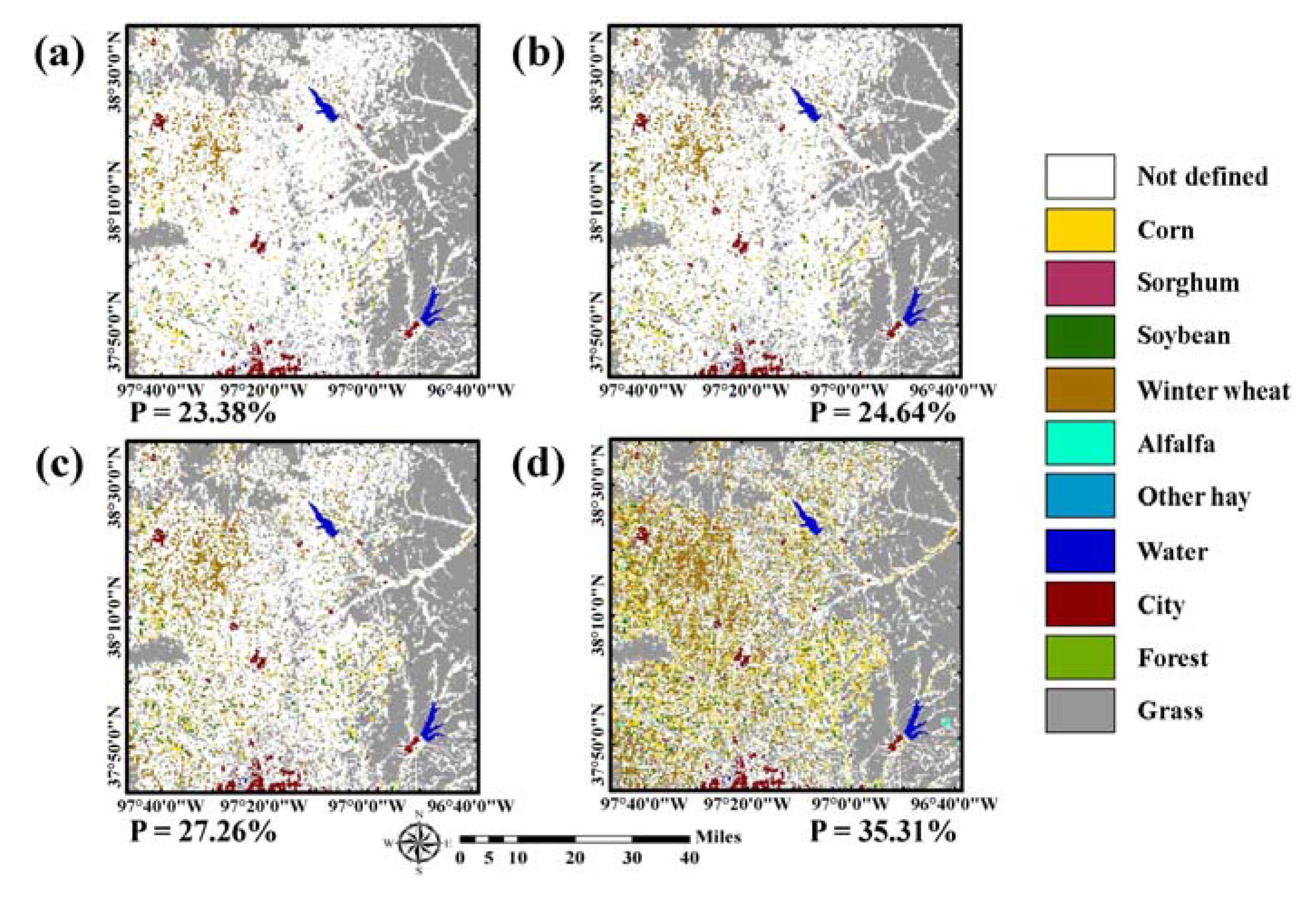
The class labels in 2015 of pixels in which sequential patterns of land-cover changes between 2010 and 2014 matched to the 21 rules were predicted as the corresponding labels of the rightmost column in Table 3. The rule-based class label images predicted from these four different cases are given in Figure 4. By superimposing the new training data candidates on the predicted label image, the class labels of the candidates were assigned automatically. Note that the rule-based class labels were not assigned to all pixels in the study area because some sequence rules were not considered and only the most confident pixels in CDLs were used to define rule information.
As the number of CDLs used to define the sequence rule decreased, the proportion of pixels in which the class labels in 2015 could be predicted increased accordingly (e.g., 23.38% (37,415 pixels) and 35.31% (56,496 pixels) for using past five-year and two-year CDLs, respectively). The fewer the CDLs, the more areas that were assigned to certain crop types such as corn, soybean, and winter wheat. By contrast, if the number of CDLs increased, relatively few areas had the rule-based class label and many areas remained unlabeled. Note that the number of pixels with rule-based class labels is much larger than that of initial training pixels (i.e., 37,415 versus 420). These rule images were separately used for further classification procedures and their classification performance were compared.
3.2. Initial Classification Result
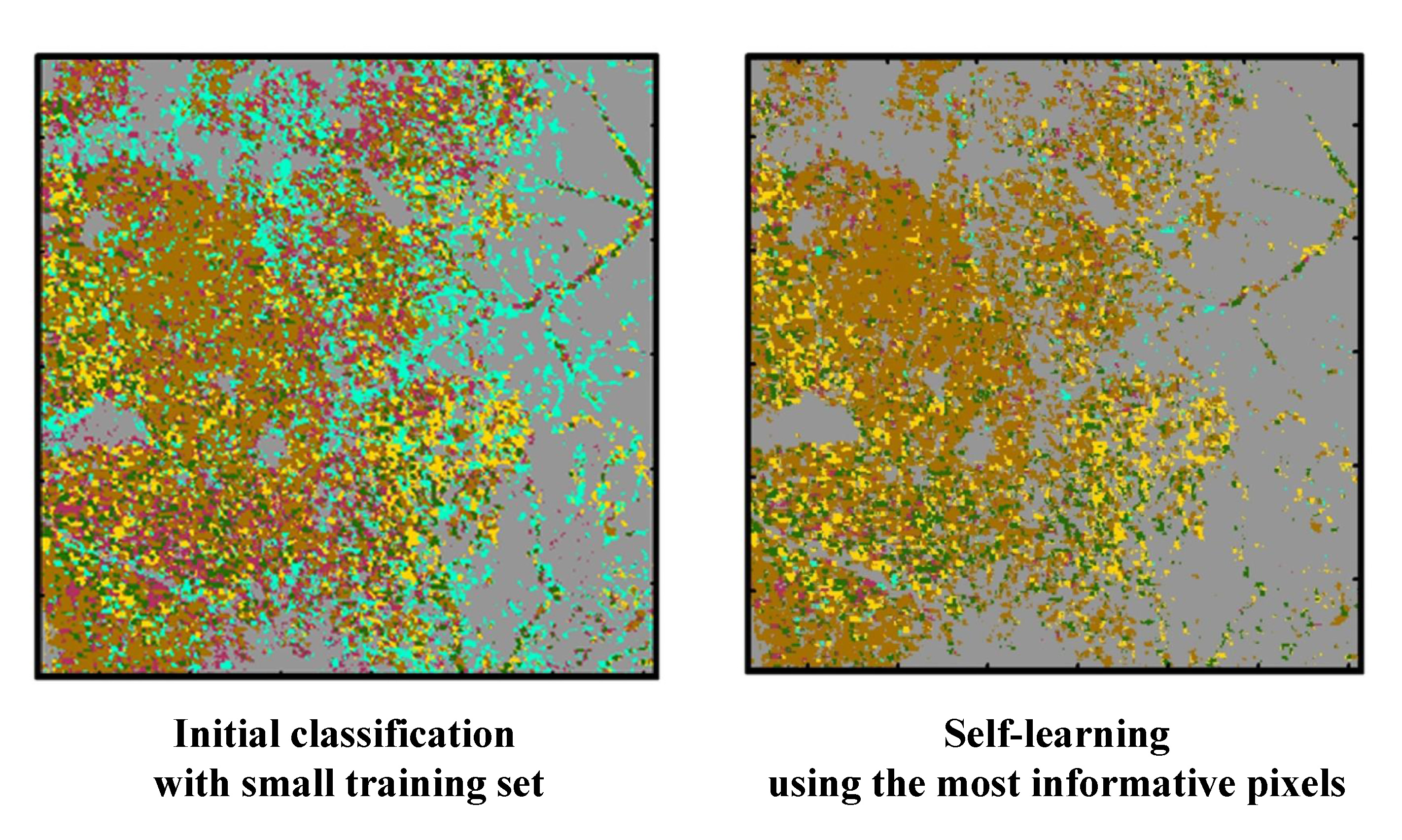
Before a self-learning procedure was employed, an initial classification was first performed using the initial training data. The qualitative and visual assessment of the initial classification results was conducted using time-series Landsat images (Figure 5). Two subareas were identified as an over-estimation of sorghum and a clustered pattern of winter wheat. The clustered pattern of winter wheat was attributed to the inclusion of more training data than the other class types in the western part of the study area. Confusion between winter wheat and alfalfa, which showed similar temporal NDVI variations in winter, could have also contributed to the clustered pattern of winter wheat in the western part. In addition, sorghum and soybean, which are the typical summer crops in Kansas, showed similar temporal NDVI variations, which led to an over-estimation of sorghum. Confusion between grain/hay and grass was also observed in the initial classification result
3.3. Self-Learning Classification Result
To select new training data candidates from the initial classification result, the BT algorithm was applied to the posteriori probabilities from a SVM classifier. The pixels that had a difference between the largest posteriori probability and the second largest posteriori probability of less than 0.05 were selected as the most informative pixels with higher uncertainty. Then, the class labels of the selected candidates were assigned to the rule-based class labels predicted from past CDLs.
If no restriction on the number of added training data was given, a large number of pixels were selected for winter wheat that is the major crop in the study area. As mentioned in Section 2.4, adding too many training data for the majority class (e.g., winter wheat) might result in the over-estimation of that class. To prevent this, another criterion was applied to restrict the number of added training data. Based on a trial and error approach, the number of training data assigned to the majority class was randomly under-sampled, and the total number of newly added training data was set to maximum 300 pixels per iteration. The variations of the number of updated training data for iterative classification are listed in Table 4. Since the number of new training pixels to be added into the previous training set was restricted, the difference of the total number of new training data was not great. However, the locations of the newly added training data were different, which led to different classification results for four CDL combination cases. Self-learning procedures for all combination cases were terminated after three or four iterations, which implied that most of pixels were mainly labeled during the first three or four iterations, and there was no significant change in the subsequent iterations.
The classification results based on a self-learning approach are presented in Figure 6. When compared with the initial classification result in Figure 5, over-estimation of sorghum and grain/hay was greatly reduced in the four classification results. The four classification results showed similar patterns overall: crop areas mainly in the west, and grain/hay and non-crop areas in the east. However, distributions of crop areas were locally different. In particular, over-estimation of soybean and under-estimation of grain/hay were observed in the two-year CDLs classification result, compared with the others. This could be attributed to the fact that the number of new training pixels assigned to alfalfa and other hay was relatively smaller than that of other CDL combination cases, as shown in Table 4. Conversely, sorghum was under-estimated in the five-year CDLs classification result. Therefore, it is expected that these different classification patterns from four CDL combination cases would result in the different classification accuracy assessment results.
3.4. Accuracy Assessment
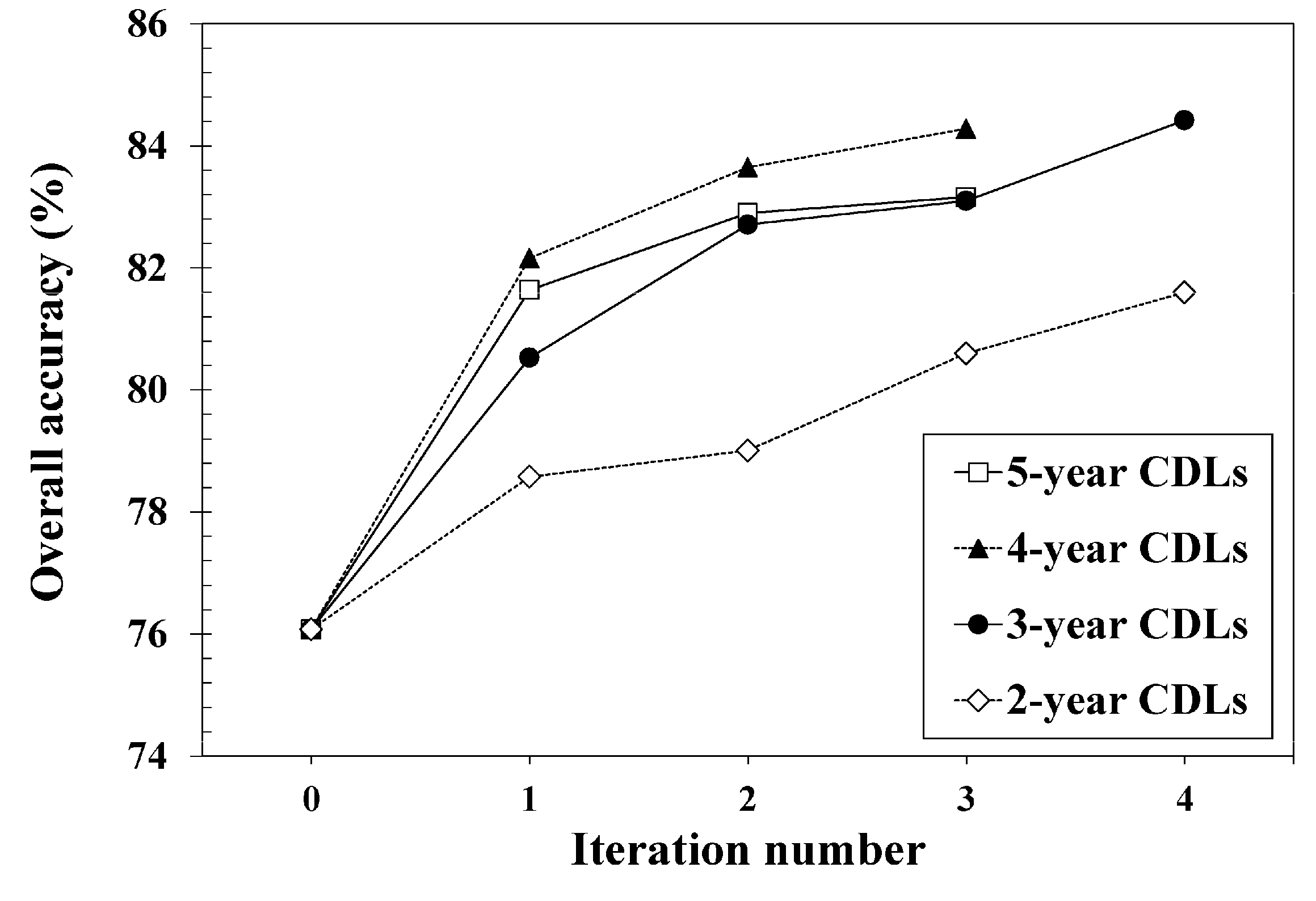
For the classification accuracy assessment, accuracy statistics such as overall accuracy, Kappa coefficient, and class-wise accuracy were computed by comparing the classification result and the reference data set in Table 2. Figure 7 shows the variations of overall accuracy for each iteration of different CDL combination cases. As shown in Figure 7, the overall accuracy increased as the number iterations increased. As a result, the self-learning approach presented in this study gave a better overall accuracy than the initial SVM classification for all different CDL combination cases. An increase of about 5.52 to 8.34 percentage points in overall accuracy was obtained by adding new training data with rule-based class labels. Based on a McNemar test [44], the improvement of overall accuracy was statistically significant at the 5% significance level. When comparing the overall accuracy values of different CDL combination cases, the best and worst (84.42% versus 81.60%) were obtained from the three-year CDLs and two-year CDLs, respectively. The case of the four-year CDL completed with fewer iterations, yet appeared to be on a trajectory to compete with the case of the 3-year CDLs which showed the best classification accuracy.
The confusion matrices for the initial classification and self-learning classification with past CDLs are listed in Table 5. Table 6 also summarizes the accuracy statistics, including overall accuracy, Kappa coefficient, and class-wise accuracy, with respect to the initial classification and the four different CDL combination cases.
As indicated in Figure 7 and Table 6, overall, adding new training data via self-learning showed the best overall accuracy and Kappa coefficient. Except for producer’s accuracy for sorghum and grain/hay and user’s accuracy for non-crop, the class-wise accuracy for the self-learning approach is superior to that for the initial classification.
Despite the poorest overall accuracy, the initial classification result gave relatively higher producer’s accuracy for sorghum and grain/hay, but the accuracy was relatively lower than other classes. As sorghum and grain/hay are minority classes in the study area, their highest producer’s accuracy could not lead to the significant improvement in overall accuracy. As shown in Figure 5 (e.g., northern and eastern parts in the study area), over-estimation of those classes decreased omission errors and resulted in this high producer’s accuracy. However, user’s accuracy (the probability that the probability that a pixel classified into a given class represents the actual class [45]) was very low for sorghum and grain/hay, which indicates very poor reliability of these two classes in the initial classification map. Most pixels of these two classes were misclassified into soybean or grass, as shown in Table 5. The accuracy for these two classes was improved by adding new training data. For sorghum, the case of the five-year CDLs showed a significant increase of approximately 56.80 percentage points in user’s accuracy. The most significant improvement of about 29.51 percentage points in user’s accuracy for grain/hay was also achieved when using past five-year CDLs. Producer’s accuracy of non-crop was the highest in the initial classification result. Despite the best accuracy of non-crop in the initial classification, this accuracy was mainly due to under-estimation of non-crop areas in the classification (see the confusion matrix in Table 5). Meanwhile, improved accuracy of major crops such as winter wheat, corn, and soybean were obtained from self-learning with past CDLs and led to the significant improvement in overall accuracy, compared with the initial classification. In summary, the improved overall accuracy of the self-learning approach was attributed to both an increase of the number of majority classes that were correctly classified and the decrease of misclassification of sorghum and grain/hay.
When the accuracy of self-learning classification with different CDL combination cases was compared, the self-learning with the five-year CDLs did not show the best classification accuracy. The case of the three-year CDLs showed the best overall accuracy and Kappa coefficient, and the case of the four-year CDLs was the second best. The poorest overall accuracy was obtained from the case of the two-year CDLs. In addition, there was no one CDL combination case where class-wise accuracy was always superior to the initial classification across all classes. Improved classification of each case resulted from the contribution of different land-cover types. In the case of the three-year CDLs, an increase of correctly classified pixels of corn and soybean led to the best overall accuracy. The second best overall accuracy in the case of the four-year CDLS was mainly due to correct classification of soybean and non-crop. An improvement in classification accuracy of cases of the five-year and two-year CDLs, compared to the initial classification, was attributed to an increase of correct classification of winter wheat and non-crop, respectively.
The core component of the self-learning approach is to derive rule-based class labels from sequential land-cover patterns in order to assign predefined class labels to the candidates for new training data. Thus, the accuracy of the predefined class label greatly affects the classification performance. To investigate this effect, further analysis was conducted by analyzing the accuracy of rule-based class labels derived from past CDLs in Figure 4. Since the true land-cover map (i.e., the CDL in 2015) was available, the rule-based class labels were directly compared with it.
The accuracy assessment results of rule-based class labels are listed in Table 7. Except for the case of the two-year CDLs, the overall accuracy of all cases was very high. As the number of CDLs for deriving sequential land-cover patterns increased, the corresponding accuracy of the rule-based class labels also increased. However, this high overall accuracy was obtained by the contribution of very high accuracy of non-crop which is one of majority classes in the study area. Regardless of different CLD combination cases, non-crop and sorghum showed the best and worst accuracy values, respectively. Unlike the rules on crop rotations, non-crop was unambiguously predicted to remain unchanged from the unique sequence rule, which led to the most accuracy of the rule-based label of non-crop. The decrease in the class-wise accuracy for crops in different CDL combination cases was due to the fact that sequential patterns of land-cover changes derived from past land-cover maps during too short a period (e.g., the two-year CDLs) were not sufficient to generate accurate rule-based class labels.
Despite the best accuracy of rule-based class labels of the five-year CDLs, however, the best classification accuracy was not obtained. This result can be attributed to the number of pixels that were assigned to rule-based class labels. The more land-cover maps that were used resulted in fewer pixels having rule-based class labels (see Figure 4). This was because more strict and stable rules were only extracted in cases that used more past-land cover maps. Although some candidate pixels with higher uncertainty were selected, their class labels cannot be assigned because no rule-based class labels were available at those pixels. As the most uncertain candidates were ignored, less uncertain candidate pixels might be selected as new training data. As a result, the selected training data might not be informative pixels. To verify these explanations, the interquartile range (IQR) of ∆P in Equation (2) at new training pixels was computed to measure the spread of uncertainty (Table 8). The smaller IQR implies the selection of more uncertain pixels with lower ∆P. As expected, the case of the five-year CDLs did not show the smallest IQR values for all classes. The smallest IQRs for corn and soybean in the case of the three-year CDLs indicate that the most informative pixels with higher uncertainty were selected as new training data, resulting in an improvement of accuracy for corn and soybean, and the best overall accuracy. From these interpretation results, the three-year CDLs were efficient for the study area because the accuracy was similar or better than the other cases. To derive a guideline on the selection of the optimal number of past land-cover maps, it is necessary to conduct more experiments on other sites using the different temporal length.
Based on all accuracy evaluation results, it can be concluded that by adding the most informative pixels with rule-based class labels, the decision boundary could be positively revised, consequently leading to an accuracy improvement. It was also found that the selection of the most informative pixels was more important for classification performance than the accuracy of rule-based class labels.
4. Discussion
4.1. Active Learning Versus Self-Learning
AL requires analyst intervention for labeling of the most informative pixels to be used for further classification. Similarly, the self-learning approach also selects pixels with high uncertainty as the most informative ones, but the class labels of the most informative pixels are defined from unique sequence rules of time-series past land-cover maps, without any analyst intervention. Thus, manual labeling load can be reduced, which is the main advantage of the self-learning approach. When classification is conducted for large areas (e.g., state or country units) or inaccessible areas, this advantage can be greatly highlighted. However, the self-learning approach does not always aim at obtaining better classification accuracy than AL because in some cases, manual labeling by analyst might be more accurate than automatic labeling in the self-learning approach.
To investigate how classification performance of self-learning is compatible with AL, an additional comparative experiment was conducted. To mimic analyst intervention, manual labeling by analyst was replaced by defining the class label of the most informative pixels to that of corresponding pixels in the 2015 CDL. The same rule for the selection of informative pixels in the self-learning approach was also applied to AL for a fair comparison. The overall accuracy and Kappa coefficient of the AL classification result were 84.99% and 0.757, respectively. When we compared these accuracy statistics of AL with self-learning with the three-year CDLs that showed the best accuracy, the difference in overall accuracy was only 0.57 percentage points (84.99% versus 84.42%). The Kappa coefficient of AL was also very similar to that of self-learning (0.757 versus 0.759). Therefore, the classification accuracy of self-learning, which is compatible to that of AL, confirms the effectiveness of the presented approach in this study.
4.2. Generation of Sequence Rules
The generation of reliable sequence rules from past land-cover maps is essential in the self-learning approach. This study applied a heuristic approach to predict the class labels of candidates for new training data. Recently, a machine learning approach was presented to build rules on crop rotations for early crop type mapping before the crop season [46]. A Markov logic network (MLN), which can combine learning from data with expert knowledge, was applied to model crop rotations. The assessment results based on different temporal length and spatial coverages revealed that the MLN showed an accuracy of up to 60%, particularly the good prediction accuracy even for a large region with heterogeneous climatic conditions and soils. In this study, a heuristic approach for the rule generation has been tested on a relatively small area. From our previous study in Illinois State [19], the rule-based class labels, which were combined with the AL-based classification results, could contribute to an improvement in classification accuracy in a large area, which indicates the applicability of rule information. Similar to the approach in Osman et al. [46], we will test whether the rules built from data in a small area can be transferred to other landscapes or large areas with diverse crop rotations, as well as the applicability of the MLN. Since a wrong label assignment greatly affects classification performances [47], the effects of class label noise and the accuracy of existing land-cover maps should also be investigated.
4.3. Practical Issues
For crop classification, annual change patterns should be used in order to properly account for various cropping systems. However, from a practical viewpoint, the collection of many consecutive annual land-cover maps is a demanding task, and not always possible. If limited land-cover maps are available, or if the time interval between sequential land-cover maps is more than two years, another approach within the self-learning framework should be developed. Instead of using deterministic hard class labels, a probabilistic approach based on transition probability can be applied. In terms of temporal contextual information, the transition probabilities between considered land-cover classes can be defined using expert knowledge. These probabilities can then be combined with the conditional probabilities based on spectral or scattering features within a probabilistic framework. If this probabilistic approach is combined with the self-learning approach, errors from rule-based class labels could be reduced. Future studies will investigate these aspects.
Other practical issue is regarding the selection of new training pixels from candidates. To alleviate the bias towards majority classes, new training pixels were selected from random under-sampling. For the comparison purposes, under-sampling of pixels with highest uncertainty was tested additionally. The candidate pixels were first sorted in a descending order by their uncertainty values and the pixels with highest uncertainty were then selected as new training pixels. When past three CDLs were used for the rule generation, the overall accuracy of this different under-sampling approach was 81.44%, which is slightly lower than that of random under-sampling (84.42%). This different classification accuracy is due to the number and class types of newly added training pixels. Relatively many pixels for sorghum which has the lower accuracy of rule-based class labels were selected as new training pixels, whereas fewer pixels for winter wheat and non-crops with high accuracy were selected. This different selection of new training pixels resulted in the lower classification accuracy. Despite the relatively higher accuracy of random under-sampling, majority classes still affected the classification accuracy, as mentioned in Section 3.4. To avoid selecting redundant pixels, the representativeness and diversity of the most uncertain pixels should be considered as criteria for the identification of the most informative pixels. To this end, entropy and spatial density measures, and clustering can be applied [48,49]. The application of these criteria will be tested within a self-learning framework.
5. Conclusions
A self-learning classification approach, which can select the most informative labeled pixels as new training data, was presented in this study. The proposed approach differs from the AL approach in that no analyst intervention was required. The class labels for new candidate pixels were predicted from representative sequence rules selected from sequential change patterns of past land-cover maps. A classification experiment in crop cultivation areas demonstrated that this method could be used to properly define the class labels of unlabeled informative pixels. By progressively adding these informative labeled pixels into the training data, misclassification based purely on spectral information from a small number of training data could be greatly reduced, and higher classification accuracy was achieved. To strengthen the advantage of the self-learning approach, more extensive classification experiments in other regions with a wide variety of land-cover types and climatic conditions and different availability of past land-cover maps will be included in future work.
Acknowledgments
This work was carried out with the support of “Cooperative Research Program for Agriculture Science & Technology Development (Project No. PJ009978),” Rural Development Administration, Republic of Korea. The authors thank three anonymous reviewers for providing invaluable comments on the original manuscript.
Author Contributions
Yeseul Kim and No-Wook Park designed this study. Yeseul Kim performed data processing and prepared the draft of this manuscript. No-Wook Park contributed to methodological developments and edited the manuscript. Kyung-Do Lee made important contributions to interpretations of crop rotations and classification results.
Conflicts of Interest
The authors declare no conflict of interest.
References
- Wardlow, B.D.; Egbert, S.L. Large-area crop mapping using time-series MODIS 250 m NDVI data: An assessment for the U.S. Central Great Plains. Remote Sens. Environ. 2008, 112, 1096–1116. [Google Scholar] [CrossRef]
- Corcoran, J.M.; Knight, J.F.; Gallant, A.L. Influence of multi-temporal remotely sensed and ancillary data on the accuracy of random forest classification of wetlands in Northern Minnesota. Remote Sens. 2013, 5, 3212–3238. [Google Scholar] [CrossRef]
- Jia, K.; Liang, S.; Wei, X.; Yao, Y.; Su, Y.; Jiang, B.; Wang, X. Land cover classification of Landsat data with phenological features extracted from time series MODIS NDVI data. Remote Sens. 2014, 6, 11518–11532. [Google Scholar] [CrossRef]
- Kong, F.; Li, X.; Wang, H.; Xie, D.; Li, X.; Bai, Y. Land cover classification based on fused data from GF-1 and MODIS NDVI time series. Remote Sens. 2016, 8, 741. [Google Scholar] [CrossRef]
- Park, N.-W.; Kyriakidis, P.C.; Hong, S. Spatial estimation of classification accuracy using indicator kriging with an image-derived ambiguity index. Remote Sens. 2016, 8, 320. [Google Scholar] [CrossRef]
- Walter, V.; Fritsch, D. Automatic verification of GIS data using high resolution multispectral data. Int. Arch. Photogramm. Remote Sens. 1998, 32, 485–490. [Google Scholar]
- Waske, B.; Benediktsson, J.A. Fusion of support vector machines for classification of multisensor data. IEEE Trans. Geosci. Remote Sens. 2007, 45, 3858–3866. [Google Scholar] [CrossRef]
- Attarchi, S.; Gloaguen, R. Classifying complex mountainous forests with L-band SAR and Landsat data integration: A comparison among different machine learning methods in the Hyrcanian forest. Remote Sens. 2014, 6, 3624–3647. [Google Scholar] [CrossRef]
- Gessner, U.; Machwitz, M.; Esch, T.; Tillack, A.; Naeimi, V.; Kuenzer, C.; Dech, S. Multi-sensor mapping of West African land cover using MODIS, ASAR and TanDEM-X/TerraSAR-X data. Remote Sens. Environ. 2015, 164, 282–297. [Google Scholar] [CrossRef]
- Heumann, B.W. An object-based classification of Mangroves using a hybrid decision tree-support vector machine approach. Remote Sens. 2011, 3, 2440–2460. [Google Scholar] [CrossRef]
- Sonobe, R.; Tani, H.; Wang, X.; Kobayashi, N.; Shimamura, H. Random forest classification of crop type using multi-temporal TerraSAR-X dual-polarimetric data. Remote Sens. Lett. 2014, 5, 157–164. [Google Scholar] [CrossRef]
- Wieland, M.; Pittore, M. Performance evaluation of machine learning algorithms for urban pattern recognition from multi-spectral satellite images. Remote Sens. 2014, 6, 2912–2939. [Google Scholar] [CrossRef]
- Zhu, X. Semi-Supervised Learning Literature Survey; Technical Report 1530; Department of Computer Sciences, University of Wisconsin-Madison: Madison, WI, USA, 2005. [Google Scholar]
- Settles, B. Active Learning Literature Survey; Technical Report 1648; Department of Computer Sciences, University of Wisconsin-Madison: Madison, WI, USA, 2010. [Google Scholar]
- Tuia, D.; Pasolli, E.; Emery, W.J. Using active learning to adapt remote sensing image classifiers. Remote Sens. Environ. 2011, 115, 2232–2242. [Google Scholar] [CrossRef]
- Ruiz, P.; Mateos, J.; Camps-Valls, G.; Molina, R.; Katsaggelos, A.K. Bayesian active remote sensing image classification. IEEE Trans. Geosci. Remote Sens. 2014, 52, 2186–2196. [Google Scholar] [CrossRef]
- Huang, X.; Weng, C.; Lu, Q.; Feng, T.; Zhang, L. Automatic labeling and selection of training samples for high-resolution remote sensing image classification over urban areas. Remote Sens. 2015, 7, 16024–16044. [Google Scholar] [CrossRef]
- Wan, L.; Tang, K.; Li, M.; Zhong, Y.; Qin, A.K. Collaborative active and semisupervised learning for hyperspectral remote sensing image classification. IEEE Trans. Geosci. Remote Sens. 2015, 53, 2384–2396. [Google Scholar] [CrossRef]
- Kim, Y.-S.; Yoo, H.-Y.; Park, N.-W.; Lee, K.-D. Classification of crop cultivation areas using active learning and temporal contextual information. J. Korean Assoc. Geogr. Inf. Stud. 2015, 18, 76–88. (In Korean) [Google Scholar] [CrossRef]
- Bruzzone, L.; Persello, C. A novel context-sensitive semisupervised SVM classifier robust to mislabeled training samples. IEEE Trans. Geosci. Remote Sens. 2009, 47, 2142–2154. [Google Scholar] [CrossRef]
- Uhlmann, S.; Kiranyaz, S.; Gabbouj, M. Semi-supervised learning for ill-posed polarimetric SAR classification. Remote Sens. 2014, 6, 4801–4830. [Google Scholar] [CrossRef]
- Chapelle, O.; Schölkopf, B.; Zien, A. Semi-Supervised Learning; The MIT Press: Cambridge, UK, 2006. [Google Scholar]
- Leng, Y.; Xu, X.; Qi, G. Combining active learning and semi-supervised learning to construct SVM classifier. Knowl.-Based Syst. 2013, 44, 121–131. [Google Scholar] [CrossRef]
- Muñoz-Marí, J.; Tuia, D.; Camps-Valls, G. Semisupervised classification of remote sensing images with active queries. IEEE Trans. Geosci. Remote Sens. 2012, 50, 3751–3763. [Google Scholar] [CrossRef]
- Dópido, I.; Li, J.; Marpu, P.R.; Plaza, A.; Dias, J.M.B.; Benediktsson, J.A. Semisupervised self-learning for hyperspectral image classification. IEEE Trans. Geosci. Remote Sens. 2013, 51, 4032–4044. [Google Scholar] [CrossRef]
- Blum, A.; Mitchell, T. Combining Labeled Data and Unlabeled Data with Co-training. In Proceedings of the Eleventh Annual Conference on Computational Learning Theory, Madison, WI, USA, 24–26 July 1998; pp. 92–100. [Google Scholar]
- Boryan, C.; Yang, Z.; Mueller, R.; Craig, M. Monitoring US agriculture: The US department of agriculture, national statistics service, cropland data layer program. Geocarto Int. 2011, 26, 341–358. [Google Scholar] [CrossRef]
- CropScape. Available online: https://nassgeodata.gmu.edu/CropScape (accessed on 1 March 2017).
- Wardlow, B.D.; Egbert, S.L. A comparison of MODIS 250-m EVI and NDVI data for crop mapping: A case study for southwest Kansas. Int. J. Remote Sens. 2010, 31, 805–830. [Google Scholar] [CrossRef]
- Conrad, C.; Colditz, R.R.; Dech, S.; Klein, D.; Vlek, P.L.G. Temporal segmentation of MODIS time series for improving crop classification in Central Asian irrigation systems. Int. J. Remote Sens. 2011, 32, 8763–8778. [Google Scholar] [CrossRef]
- Kim, Y.; Park, N.-W.; Hong, S.; Lee, K.; Yoo, H.Y. Early production of large-area crop classification map using time-series vegetation index and past crop cultivation patterns. Korean J. Remote Sens. 2014, 30, 493–503. (In Korean) [Google Scholar] [CrossRef]
- Chen, J.; Jönsson, P.; Tamura, M.; Gu, Z.; Matsushita, B.; Eklundh, L. A simple method for reconstructing a high-quality NDVI time-series data set based on the Savitzky-Golay filter. Remote Sens. Environ. 2004, 91, 332–344. [Google Scholar] [CrossRef]
- Melgani, F.; Bruzzone, L. Classification of hyperspectral remote sensing images with support vector machines. IEEE Trans. Geosci. Remote Sens. 2004, 42, 1778–1790. [Google Scholar] [CrossRef]
- Mathur, A.; Foody, G.M. Crop classification by support vector machine with intelligently selected training data for an operational application. Int. J. Remote Sens. 2008, 29, 2227–2240. [Google Scholar] [CrossRef]
- Vapnik, V. Statistical Learning Theory; Wiley: New York, NY, USA, 1998. [Google Scholar]
- Wu, T.-F.; Lin, C.-J.; Weng, R.C. Probability estimates for multi-class classification by pairwise coupling. J. Mach. Learn. Res. 2004, 5, 975–1005. [Google Scholar]
- Tuia, D.; Ratle, F.; Pacifici, F.; Kanevski, M.F.; Emery, W.J. Active learning methods for remote sensing image classification. IEEE Trans. Geosci. Remote Sens. 2009, 47, 2218–2232. [Google Scholar] [CrossRef]
- Tuia, D.; Volpi, M.; Copa, L.; Kanevski, M.; Muñoz-Marí, J. A survey of active learning algorithms for supervised remote sensing image classification. IEEE J. Sel. Top. Signal Process. 2011, 5, 606–617. [Google Scholar] [CrossRef]
- Li, J.; Bioucas-Dias, J.M.; Plaza, A. Hyperspectral image segmentation using new Bayesian approach with active learning. IEEE Trans. Geosci. Remote. 2011, 49, 3947–3960. [Google Scholar] [CrossRef]
- Luo, T.; Kramer, K.; Goldgof, D.B.; Hall, L.O.; Samson, S.; Remsen, A.; Hopkins, T. Active learning to recognize multiple types of plankton. J. Mach. Learn. Res. 2005, 6, 589–613. [Google Scholar]
- Acosta-Martínez, V.; Mikha, M.M.; Vigil, M.F. Microbial communities and enzyme activities in soils under alternative crop rotations compared to wheat-fallow for the Central Great Plains. Appl. Soil Ecol. 2007, 37, 41–52. [Google Scholar] [CrossRef]
- Culman, S.W.; DuPont, S.T.; Glover, J.D.; Buckley, D.H.; Fick, G.W.; Ferris, H.; Crews, T.E. Long-term impacts of high-input annual cropping and unfertilized perennial grass production on soil properties and belowground food webs in Kansas, USA. Agric. Ecosyst. Environ. 2010, 137, 13–24. [Google Scholar] [CrossRef]
- Wardlow, B.D.; Egbert, S.L.; Kastens, J.H. Analysis of time-series MODIS 250 m vegetation index data for crop classification in the U.S. Central Great Plains. Remote Sens. Environ. 2007, 108, 290–310. [Google Scholar] [CrossRef]
- Foody, G.M. Thematic map comparison: Evaluating the statistical significance of differences in classification accuracy. Photogramm. Eng. Remote Sens. 2008, 70, 627–633. [Google Scholar] [CrossRef]
- Lillesand, T.M.; Kiefer, R.W.; Chipman, J.W. Remote Sensing and Image Interpretation, 6th ed.; Wiley: Hoboken, NJ, USA, 2008. [Google Scholar]
- Osman, J.; Inglada, J.; Dejoux, J.-F. Assessment of a Markov logic model of crop rotation for early crop mapping. Comput. Electron. Agric. 2015, 113, 234–243. [Google Scholar] [CrossRef] [Green Version]
- Pelletier, C.; Valero, S.; Inglada, J.; Champion, N.; Sicre, C.M.; Dedieu, G. Effect of training class label noise on classification performances for land cover mapping with satellite image time series. Remote Sens. 2017, 9, 173. [Google Scholar] [CrossRef]
- He, T.; Zhang, S.; Xin, J.; Zhao, P.; Wu, J.; Xian, X.; Li, C.; Cui, Z. An active learning approach with uncertainty, representativeness, and diversity. Sci. World J. 2014, 2014, 827586. [Google Scholar] [CrossRef] [PubMed]
- Demir, B.; Minello, L.; Bruzzone, L. An effective strategy to reduce the labeling cost in the definition of training sets by active learning. IEEE Geosci. Remote Sens. Lett. 2015, 11, 79–83. [Google Scholar] [CrossRef]
Figure 1.
Location of the study area and data sets: (a) Moderate Resolution Imaging Spectroradiometer (MODIS) Normalized Difference Vegetation Index (NDVI) on 9 May 2015, at a 250 m spatial resolution and (b) cropland data layer (CDL) 2015 at a 30 m spatial resolution.
Figure 1.
Location of the study area and data sets: (a) Moderate Resolution Imaging Spectroradiometer (MODIS) Normalized Difference Vegetation Index (NDVI) on 9 May 2015, at a 250 m spatial resolution and (b) cropland data layer (CDL) 2015 at a 30 m spatial resolution.
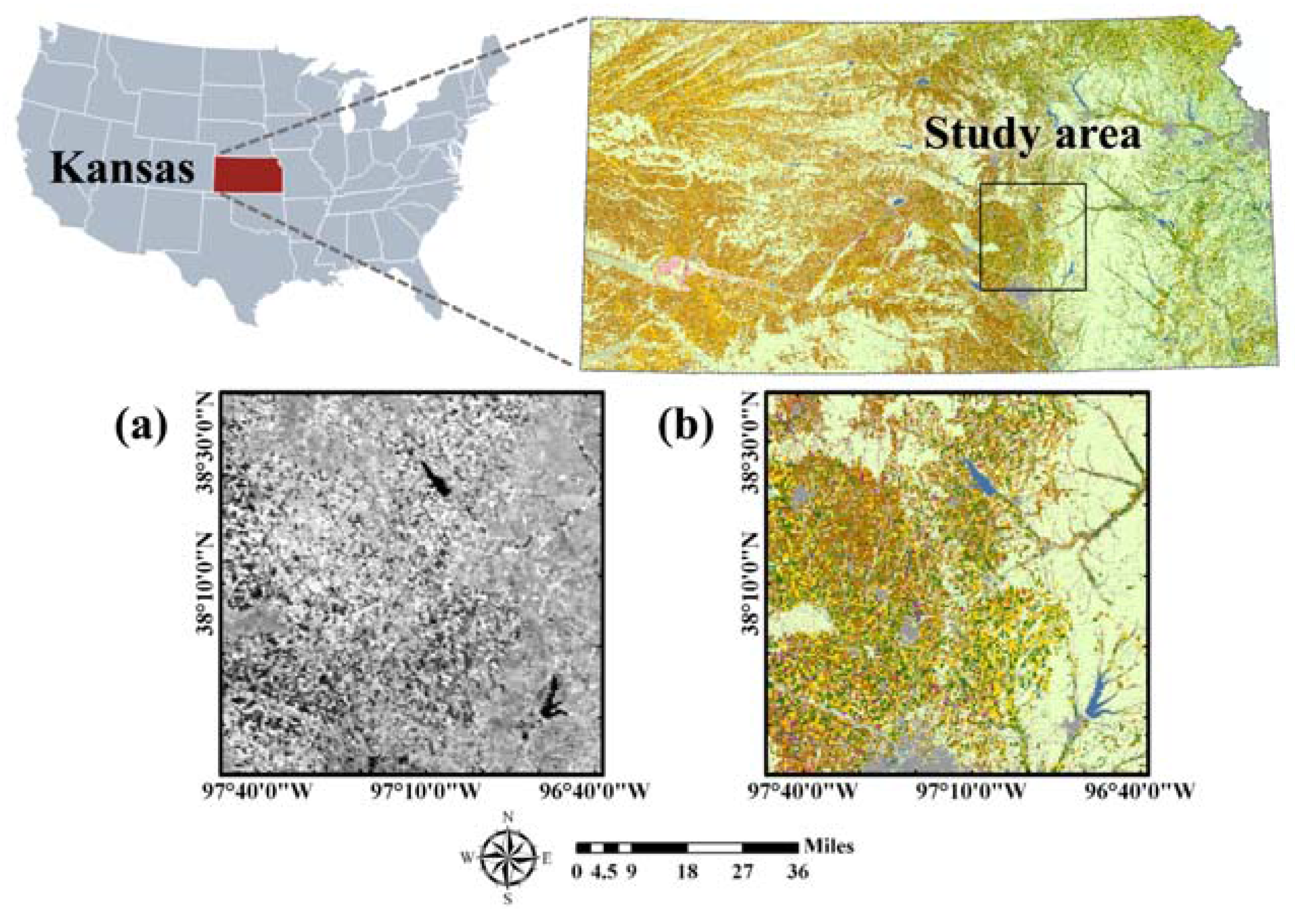
Figure 2.
Flow chart of the classification procedures presented in this study.
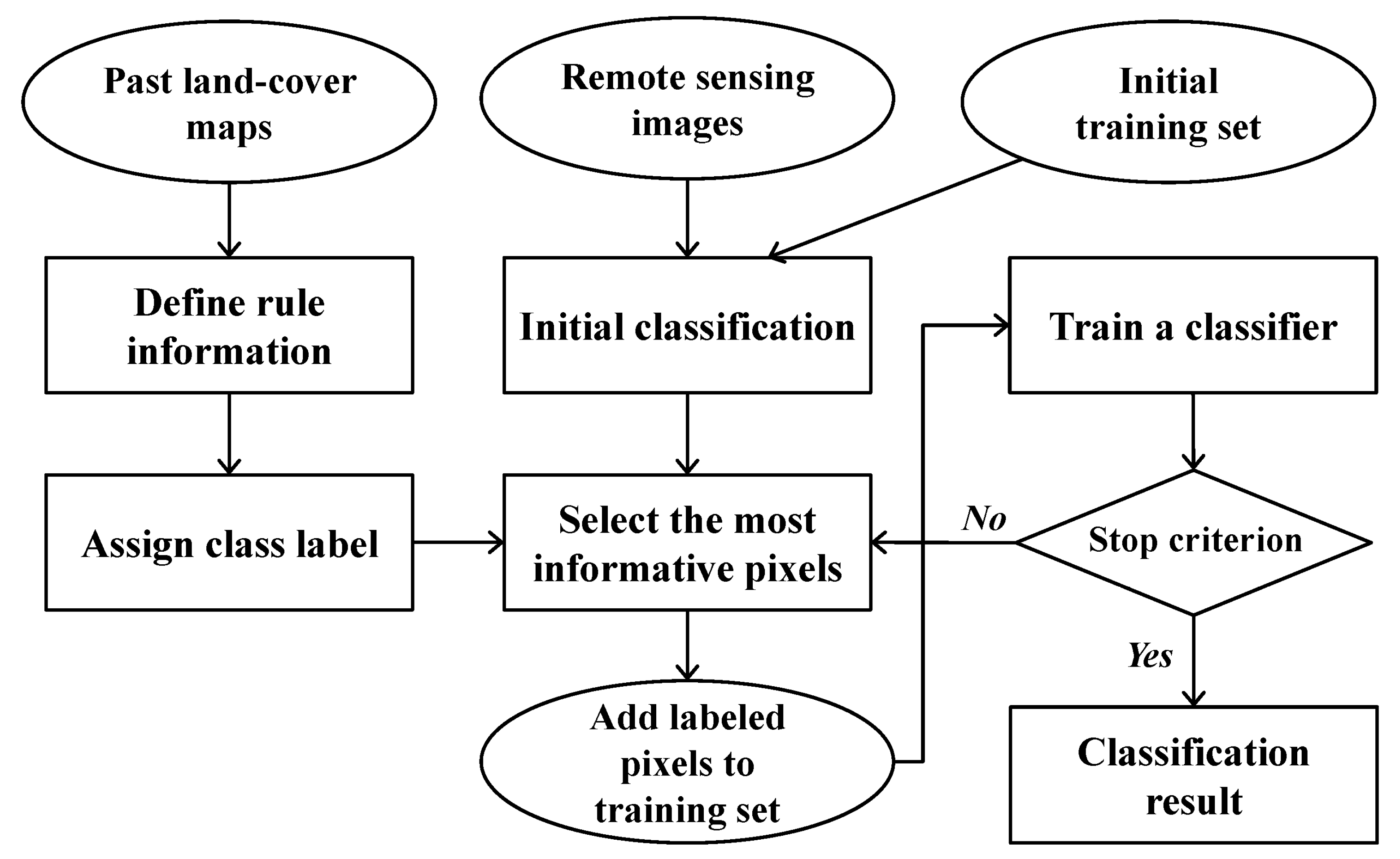
Figure 3.
Illustrations for the process of generating rule-based class labels. Past land-cover maps are stacked and compared, where Tn is the reference year under consideration.
Figure 3.
Illustrations for the process of generating rule-based class labels. Past land-cover maps are stacked and compared, where Tn is the reference year under consideration.
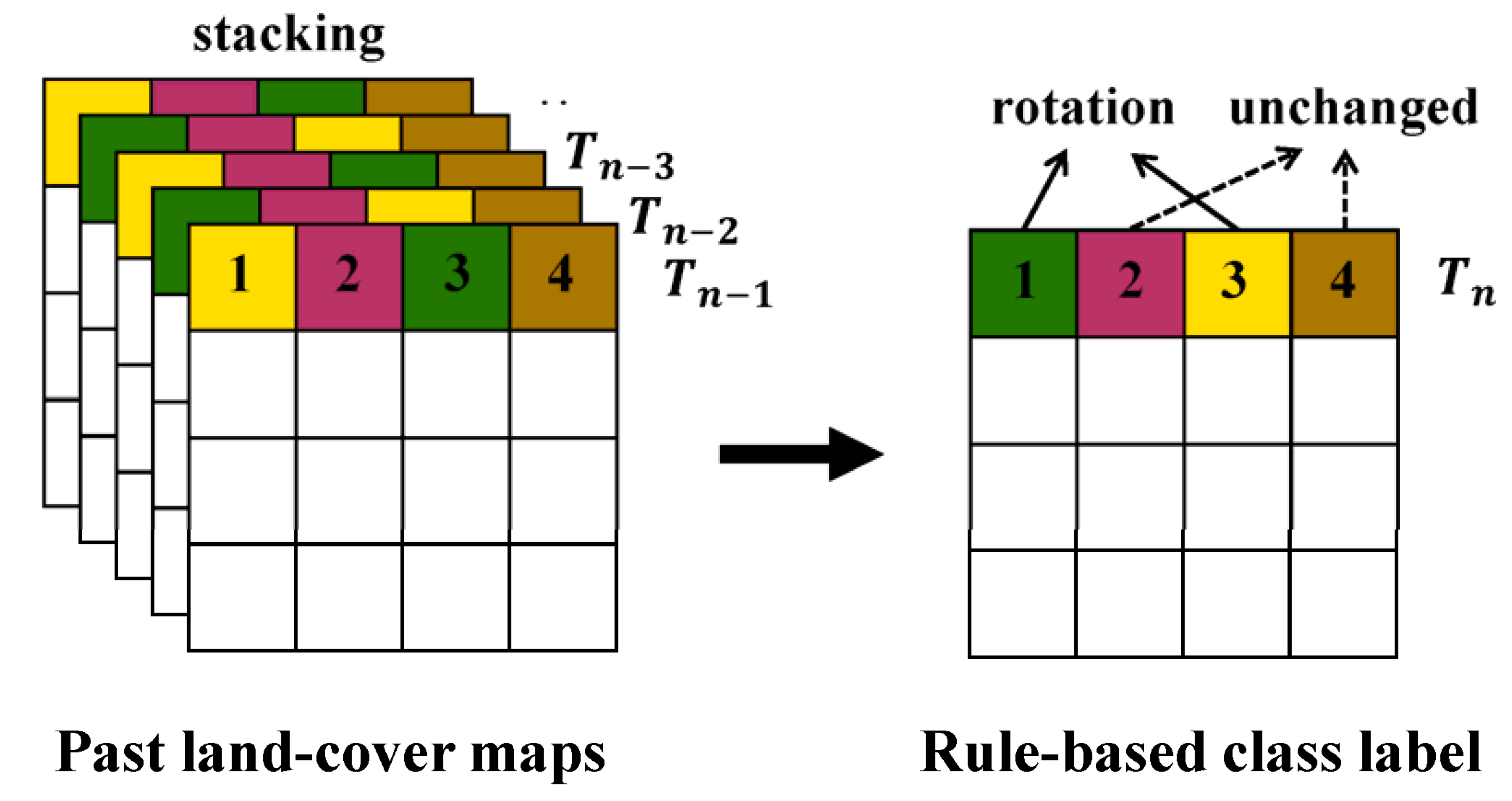
Figure 4.
Rule-based class label images predicted from past CDLs: (a) 5-year (2010 to 2014), (b) 4-year (2011 to 2014), (c) 3-year (2012 to 2014), and (d) 2-year (2013 to 2014). P (the percentage value below each predicted class label image) denotes the proportion of pixels in which the class label for 2015 could be predicted.

Figure 5.
Initial classification result, and its visual comparison with Landsat images in two subareas.
Figure 5.
Initial classification result, and its visual comparison with Landsat images in two subareas.
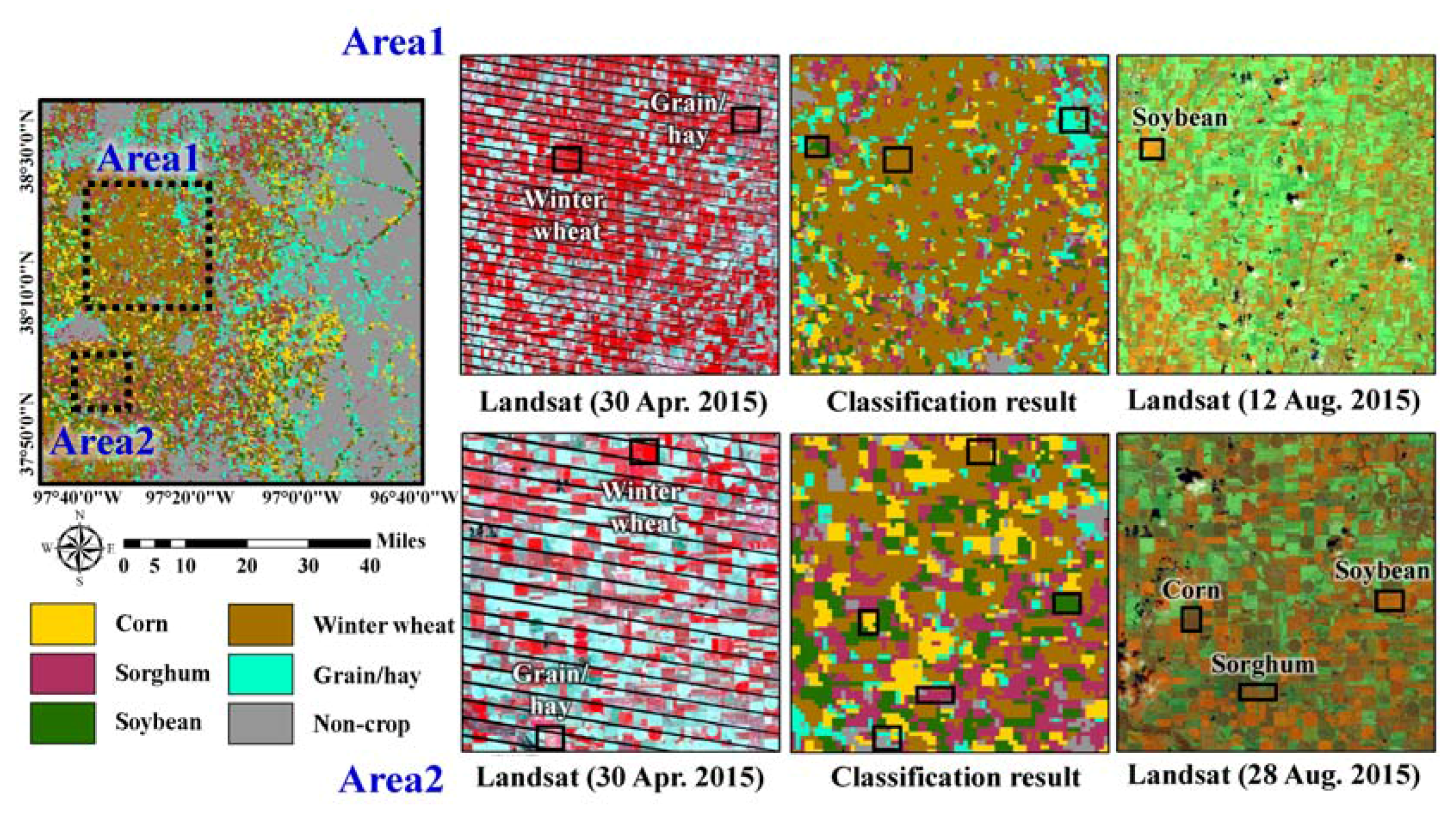
Figure 6.
Final classification results of a self-learning approach with different past CDLs: (a) 5-year (2010 to 2014); (b) 4-year (2011 to 2014); (c) 3-year (2012 to 2014); and (d) 2-year (2013 to 2014).
Figure 6.
Final classification results of a self-learning approach with different past CDLs: (a) 5-year (2010 to 2014); (b) 4-year (2011 to 2014); (c) 3-year (2012 to 2014); and (d) 2-year (2013 to 2014).
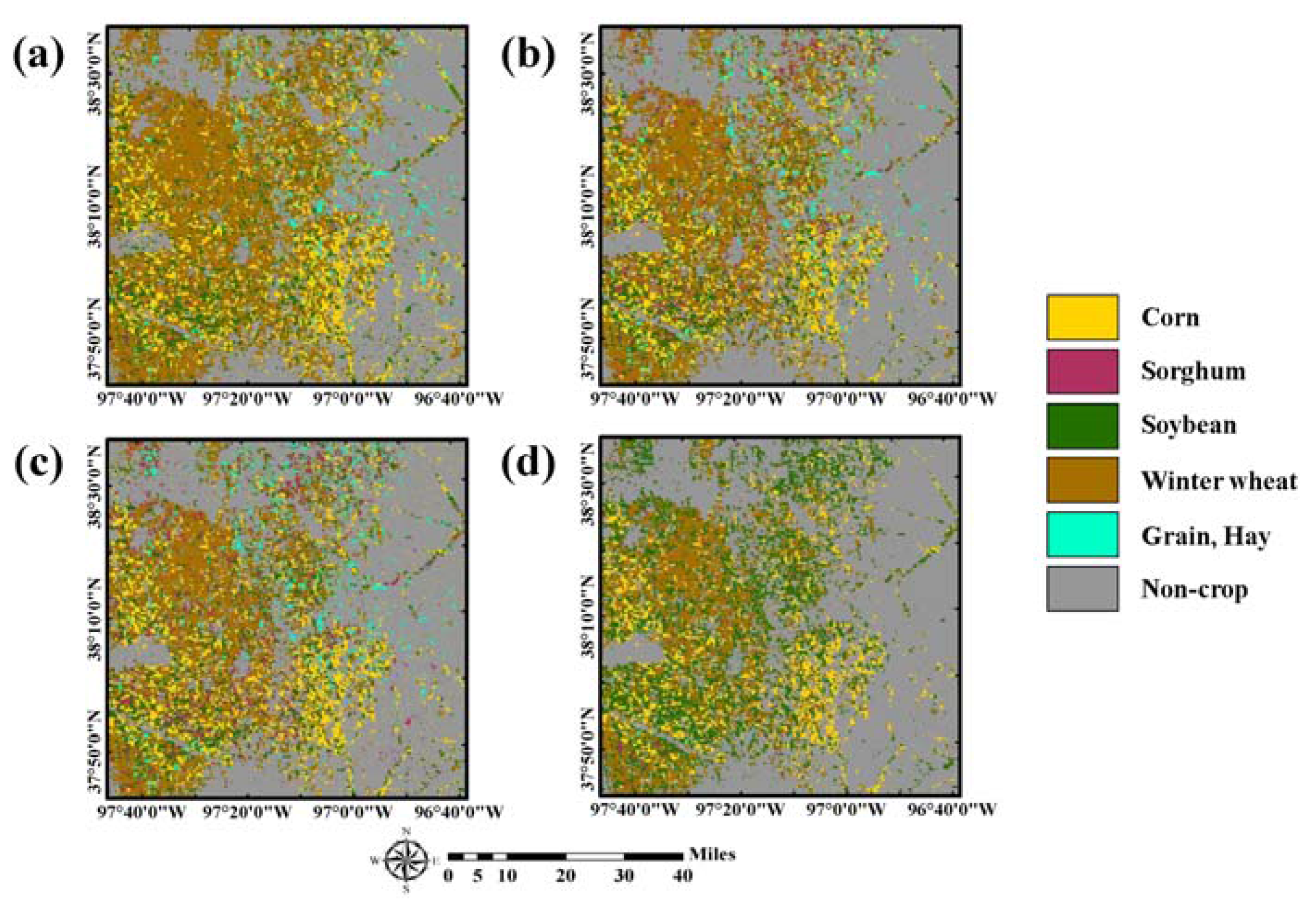
Figure 7.
Overall accuracy versus the iteration number for the four different CDL combination cases. Iteration 0 indicates the initial classification.
Figure 7.
Overall accuracy versus the iteration number for the four different CDL combination cases. Iteration 0 indicates the initial classification.

Table 1.
The list of class types for supervised classification and merged classes, and the number of initial training data per each class.
Table 1.
The list of class types for supervised classification and merged classes, and the number of initial training data per each class.
| No | Class | Merged Class | Number of Training Data |
|---|---|---|---|
| 1 | Corn | Corn | 45 |
| 2 | Sorghum | Sorghum | 25 |
| 3 | Soybean | Soybean | 45 |
| 4 | Winter wheat | Winter wheat | 100 |
| 5 | Alfalfa | Grain/hay | 20 |
| 6 | Other hay | Grain/hay | 15 |
| 7 | Water | Non-crop | 37 |
| 8 | City | Non-crop | 28 |
| 9 | Forest | Non-crop | 20 |
| 10 | Grass | Non-crop | 85 |
| Total | 420 | ||
Table 2.
Number of reference data.
| Class | Number |
|---|---|
| Corn | 6263 |
| Sorghum | 1864 |
| Soybean | 6016 |
| Winter wheat | 14,582 |
| Grain/hay | 651 |
| Non-crop | 34,624 |
| Total | 64,000 |
Table 3.
Sequential patterns of land-covers between 2010 and 2014 (C: corn, S: sorghum, SB: soybean, WW: winter wheat, A: alfalfa, OH: other hay, FA: fallow, W: water, U: urban, FO: forest, G: grass). The class labels in 2015 predicted from CDLs spanning the past five years are shown in bold.
Table 3.
Sequential patterns of land-covers between 2010 and 2014 (C: corn, S: sorghum, SB: soybean, WW: winter wheat, A: alfalfa, OH: other hay, FA: fallow, W: water, U: urban, FO: forest, G: grass). The class labels in 2015 predicted from CDLs spanning the past five years are shown in bold.
| No | 2010 | 2011 | 2012 | 2013 | 2014 | Predicted Label for 2015 |
|---|---|---|---|---|---|---|
| 1 | C | C | C | C | C | C |
| 2 | S | S | S | S | S | S |
| 3 | SB | SB | SB | SB | SB | SB |
| 4 | WW | WW | WW | WW | WW | WW |
| 5 | C | S | C | S | C | S |
| 6 | S | C | S | C | S | C |
| 7 | C | SB | C | SB | C | SB |
| 8 | SB | C | SB | C | SB | C |
| 9 | S | SB | S | SB | S | SB |
| 10 | WW | C | WW | C | WW | C |
| 11 | C | WW | C | WW | C | WW |
| 12 | WW | SB | WW | SB | WW | SB |
| 13 | SB | WW | SB | WW | SB | WW |
| 14 | WW | FA | WW | FA | WW | FA |
| 15 | FA | WW | FA | WW | FA | WW |
| 16 | A | A | A | A | A | A |
| 17 | OH | OH | OH | OH | OH | OH |
| 18 | W | W | W | W | W | W |
| 19 | FO | FO | FO | FO | FO | FO |
| 20 | U | U | U | U | U | U |
| 21 | G | G | G | G | G | G |
Table 4.
Number of new training data at each iteration for four different past CDL combination cases.
Table 4.
Number of new training data at each iteration for four different past CDL combination cases.
| Class | Past 5-Year CDLs | Past 4-Year CDLs | Past 3-Year CDLs | Past 2-Year CDLs | ||||||||||
|---|---|---|---|---|---|---|---|---|---|---|---|---|---|---|
| Iteration | 1 | 2 | 3 | 1 | 2 | 3 | 1 | 2 | 3 | 4 | 1 | 2 | 3 | 4 |
| Corn | 90 | 150 | 194 | 91 | 129 | 156 | 90 | 123 | 156 | 216 | 88 | 128 | 162 | 187 |
| Sorghum | 25 | 50 | 79 | 38 | 63 | 86 | 39 | 60 | 90 | 111 | 42 | 62 | 76 | 86 |
| Soybean | 90 | 150 | 195 | 90 | 132 | 167 | 91 | 128 | 165 | 217 | 86 | 126 | 162 | 182 |
| Winter wheat | 160 | 200 | 220 | 155 | 155 | 210 | 163 | 201 | 216 | 241 | 160 | 185 | 211 | 246 |
| Alfala | 26 | 36 | 72 | 36 | 56 | 74 | 35 | 45 | 55 | 73 | 35 | 43 | 43 | 63 |
| Other hay | 15 | 15 | 15 | 15 | 15 | 15 | 15 | 15 | 15 | 15 | 15 | 15 | 15 | 15 |
| City | 57 | 92 | 112 | 57 | 83 | 101 | 57 | 77 | 87 | 107 | 52 | 77 | 91 | 101 |
| Water | 47 | 72 | 107 | 53 | 93 | 118 | 50 | 95 | 105 | 130 | 62 | 96 | 116 | 126 |
| Forest | 40 | 63 | 80 | 28 | 62 | 85 | 30 | 70 | 77 | 77 | 35 | 60 | 70 | 76 |
| Grass | 170 | 192 | 227 | 157 | 192 | 222 | 150 | 180 | 228 | 267 | 145 | 205 | 255 | 269 |
| Total | 720 | 1020 | 1310 | 720 | 980 | 1234 | 720 | 994 | 1194 | 1454 | 720 | 997 | 1201 | 1351 |
Table 5.
Confusion matrices for initial classification and self-learning classification for four different CDL combination cases.
Table 5.
Confusion matrices for initial classification and self-learning classification for four different CDL combination cases.
| Initial Classification | ||||||||
|---|---|---|---|---|---|---|---|---|
| Reference | Corn | Sorghum | Soybean | Winter Wheat | Grain/Hay | Non-Crop | Sum | |
| Classification | ||||||||
| Corn | 3698 | 49 | 144 | 435 | 28 | 567 | 4921 | |
| Sorghum | 630 | 1186 | 1329 | 725 | 32 | 1223 | 5125 | |
| Soybean | 387 | 161 | 3420 | 222 | 7 | 152 | 4349 | |
| Winter wheat | 394 | 309 | 856 | 11,500 | 77 | 766 | 13,902 | |
| Grain/hay | 436 | 33 | 66 | 1333 | 469 | 3500 | 5837 | |
| Non-crop | 718 | 126 | 201 | 367 | 38 | 28,416 | 29,866 | |
| Sum | 6263 | 1864 | 6016 | 14,582 | 651 | 34,624 | 64,000 | |
| Self-learning classification with past 5-year CDLs | ||||||||
| Reference | Corn | Sorghum | Soybean | Winter Wheat | Grain/Hay | Non-Crop | Sum | |
| Classification | ||||||||
| Corn | 4596 | 124 | 524 | 308 | 35 | 1334 | 6921 | |
| Sorghum | 0 | 1020 | 92 | 124 | 0 | 40 | 1276 | |
| Soybean | 443 | 466 | 3775 | 369 | 9 | 708 | 5770 | |
| Winter wheat | 640 | 0 | 1176 | 12,938 | 166 | 1600 | 16,520 | |
| Grain/hay | 33 | 3 | 7 | 128 | 330 | 378 | 879 | |
| Non-crop | 551 | 251 | 442 | 715 | 111 | 30,564 | 32,634 | |
| Sum | 6263 | 1864 | 6016 | 14,582 | 651 | 34,624 | 64,000 | |
| Self-learning classification with past 4-year CDLs | ||||||||
| Reference | Corn | Sorghum | Soybean | Winter Wheat | Grain/Hay | Non-Crop | Sum | |
| Classification | ||||||||
| Corn | 4308 | 112 | 467 | 359 | 27 | 461 | 5734 | |
| Sorghum | 53 | 916 | 100 | 449 | 6 | 134 | 1658 | |
| Soybean | 374 | 200 | 4147 | 459 | 13 | 76 | 5269 | |
| Winter wheat | 337 | 303 | 545 | 11,372 | 66 | 781 | 13,404 | |
| Grain/hay | 62 | 5 | 15 | 435 | 326 | 304 | 1147 | |
| Non-crop | 1129 | 328 | 742 | 1508 | 213 | 32,868 | 36,788 | |
| Sum | 6263 | 1864 | 6016 | 14,582 | 651 | 34,624 | 64,000 | |
| Self-learning classification with past 3-year CDLs | ||||||||
| Reference | Corn | Sorghum | Soybean | Winter Wheat | Grain/Hay | Non-Crop | Sum | |
| Classification | ||||||||
| Corn | 5244 | 137 | 136 | 546 | 24 | 1384 | 7471 | |
| Sorghum | 124 | 1043 | 290 | 683 | 5 | 329 | 2474 | |
| Soybean | 338 | 153 | 5110 | 760 | 20 | 295 | 6676 | |
| Winter wheat | 211 | 236 | 355 | 10,431 | 41 | 465 | 11,739 | |
| Grain/hay | 42 | 8 | 23 | 619 | 333 | 285 | 1310 | |
| Non-crop | 304 | 287 | 102 | 1543 | 228 | 31,866 | 34,330 | |
| Sum | 6263 | 1864 | 6016 | 14,582 | 651 | 34,624 | 64,000 | |
| Self-learning classification with past 2-year CDLs | ||||||||
| Reference | Corn | Sorghum | Soybean | Winter Wheat | Grain/Hay | Non-Crop | Sum | |
| Classification | ||||||||
| Corn | 5099 | 76 | 496 | 321 | 19 | 270 | 6281 | |
| Sorghum | 68 | 635 | 130 | 582 | 0 | 9 | 1424 | |
| Soybean | 464 | 655 | 4651 | 3245 | 51 | 690 | 9756 | |
| Winter wheat | 201 | 168 | 336 | 8530 | 29 | 359 | 9623 | |
| Grain/hay | 1 | 1 | 0 | 22 | 13 | 3 | 40 | |
| Non-crop | 430 | 329 | 403 | 1882 | 539 | 33,293 | 36,876 | |
| Sum | 6263 | 1864 | 6016 | 14,582 | 651 | 34,624 | 64,000 | |
Table 6.
Comparison of the accuracy statistics for the different classification results. UA and PA denote user’s accuracy and producer’s accuracy, respectively. The best case is shown in bold.
Table 6.
Comparison of the accuracy statistics for the different classification results. UA and PA denote user’s accuracy and producer’s accuracy, respectively. The best case is shown in bold.
| Initial Classification | Self-Learning | |||||
|---|---|---|---|---|---|---|
| Past 5-Year CDLs | Past 4-Year CDLs | Past 3-Year CDLs | Past 2-Year CDLs | |||
| Overall accuracy | 76.08 | 83.16 | 84.28 | 84.42 | 81.60 | |
| Kappa coefficient | 0.65 | 0.74 | 0.75 | 0.76 | 0.71 | |
| Corn | PA | 59.05 | 73.38 | 68.78 | 83.73 | 81.41 |
| UA | 75.15 | 66.41 | 75.13 | 70.19 | 81.18 | |
| Sorghum | PA | 63.63 | 54.72 | 49.14 | 55.95 | 34.07 |
| UA | 23.14 | 79.94 | 55.25 | 42.16 | 44.59 | |
| Soybean | PA | 56.85 | 62.75 | 65.61 | 84.94 | 77.31 |
| UA | 78.64 | 65.42 | 78.71 | 76.54 | 47.67 | |
| Winter wheat | PA | 78.86 | 88.73 | 77.99 | 71.53 | 58.50 |
| UA | 82.72 | 78.32 | 84.84 | 88.86 | 88.64 | |
| Grain/hay | PA | 72.04 | 50.69 | 50.08 | 51.15 | 2.00 |
| UA | 8.03 | 37.54 | 28.42 | 25.42 | 32.50 | |
| Non-crop | PA | 82.07 | 88.27 | 94.35 | 92.03 | 96.16 |
| UA | 95.14 | 93.66 | 89.34 | 92.82 | 90.28 | |
Table 7.
Accuracy of rule-based class labels for four different past CDL combination cases.
| Past 5-Year CDLs | Past 4-Year CDLs | Past 3-Year CDLs | Past 2-Year CDLs | |
|---|---|---|---|---|
| Overall accuracy | 98.42 | 97.50 | 94.17 | 81.49 |
| Kappa coefficient | 0.94 | 0.92 | 0.86 | 0.69 |
| Corn | 91.25 | 86.73 | 76.27 | 52.99 |
| Sorghum | 32.35 | 51.02 | 38.08 | 21.65 |
| Soybean | 80.84 | 78.51 | 65.75 | 39.83 |
| Winter wheat | 92.42 | 89.47 | 82.02 | 65.72 |
| Grain/hay | 85.45 | 82.69 | 84.88 | 77.10 |
| Non-crop | 99.91 | 99.91 | 99.91 | 99.90 |
Table 8.
Interquartile range of uncertainty values at new training pixels for four different past CDL combination cases.
Table 8.
Interquartile range of uncertainty values at new training pixels for four different past CDL combination cases.
| Class | Past 5-Year CDLs | Past 4-Year CDLs | Past 3-Year CDLs | Past 2-Year CDLs |
|---|---|---|---|---|
| Corn | 0.256 | 0.257 | 0.153 | 0.267 |
| Sorghum | 0.184 | 0.256 | 0.208 | 0.161 |
| Soybean | 0.273 | 0.261 | 0.208 | 0.231 |
| Winter wheat | 0.321 | 0.237 | 0.349 | 0.277 |
| Grain/hay | 0.123 | 0.189 | 0.101 | 0.091 |
| Non-crop | 0.512 | 0.654 | 0.437 | 0.303 |
© 2017 by the authors. Licensee MDPI, Basel, Switzerland. This article is an open access article distributed under the terms and conditions of the Creative Commons Attribution (CC BY) license (http://creativecommons.org/licenses/by/4.0/).
Share and Cite
MDPI and ACS Style
Kim, Y.; Park, N.-W.; Lee, K.-D. Self-Learning Based Land-Cover Classification Using Sequential Class Patterns from Past Land-Cover Maps. Remote Sens. 2017, 9, 921. https://doi.org/10.3390/rs9090921
AMA Style
Kim Y, Park N-W, Lee K-D. Self-Learning Based Land-Cover Classification Using Sequential Class Patterns from Past Land-Cover Maps. Remote Sensing. 2017; 9(9):921. https://doi.org/10.3390/rs9090921
Chicago/Turabian StyleKim, Yeseul, No-Wook Park, and Kyung-Do Lee. 2017. "Self-Learning Based Land-Cover Classification Using Sequential Class Patterns from Past Land-Cover Maps" Remote Sensing 9, no. 9: 921. https://doi.org/10.3390/rs9090921
Note that from the first issue of 2016, this journal uses article numbers instead of page numbers. See further details here.