Hyperspectral Image Classification Based on Semi-Supervised Rotation Forest

Abstract

Ensemble learning is widely used to combine varieties of weak learners in order to generate a relatively stronger learner by reducing either the bias or the variance of the individual learners. Rotation forest (RoF), combining feature extraction and classifier ensembles, has been successfully applied to hyperspectral (HS) image classification by promoting the diversity of base classifiers since last decade. Generally, RoF uses principal component analysis (PCA) as the rotation tool, which is commonly acknowledged as an unsupervised feature extraction method, and does not consider the discriminative information about classes. Sometimes, however, it turns out to be sub-optimal for classification tasks. Therefore, in this paper, we propose an improved RoF algorithm, in which semi-supervised local discriminant analysis is used as the feature rotation tool. The proposed algorithm, named semi-supervised rotation forest (SSRoF), aims to take advantage of both the discriminative information and local structural information provided by the limited labeled and massive unlabeled samples, thus providing better class separability for subsequent classifications. In order to promote the diversity of features, we also adjust the semi-supervised local discriminant analysis into a weighted form, which can balance the contributions of labeled and unlabeled samples. Experiments on several hyperspectral images demonstrate the effectiveness of our proposed algorithm compared with several state-of-the-art ensemble learning approaches.

1. Introduction

Hyperspectral (HS) image classification always suffers from varieties of difficulties, such as high dimensionality, limited or unbalanced training samples, spectral variability, and mixing pixels. It is well known that increasing data dimensionality and high redundancy between features might cause problems during data analysis, for example, in the context of supervised classification. A considerable amount of literature has been published with regard to overcoming these challenges, and performing hyperspectral image classification effectively [1]. Machine learning techniques such as artificial neural networks (ANNs) [2], support vector machine (SVM) [3], multinomial logistic regression [4], active learning, semi-supervised learning [5], and other methods like hyperspectral unmixing [6], object-oriented classification [7], and the multiple classifier system [8] have been popularly investigated recently as well.

Multiple classifier system (MCS), which is also sometimes named as classifier ensemble or ensemble learning (EL) in the machine learning field, is a popular strategy for improving the classification performance of hyperspectral images by combining the predictions of multiple classifiers, thereby reducing the dependence on the performance of a single classifier [8,9,10,11]. The concept of MCS, on the other hand, does not refer to a specific algorithm but to the idea of combining outputs from more than one classifier to enhance classification accuracy [12]. These outputs may result from either the same classifier of different variants or different classifiers of the same/different training samples. Previous studies have demonstrated both theoretically and experimentally that one of the main reasons for the success of ensembles is the diversity among the individual learners (namely the base classifiers) [13], because combining similar classification results would not further improve the accuracy.

MCSs have been widely applied to HS remote sensing image classification. Two approaches for constructing classifier ensembles are perceived as “classic”, bagging and boosting [14,15], and afterwards numerous algorithms were successively derived from them. Bagging creates many classifiers with each base learner trained by a new bootstrapped training data set [16]. Boosting processes the data with iterative retraining, and concentrates on the difficult samples, with the goal of correctly classifying these samples in the next iteration [17,18]. Ho [19] proposed random subspace ensembles, which used random subsets of features instead of the entire feature set for each individual classifier. The rationale of the random subspace is to break down a complex high dimensional problem into several lower dimensional problems, thereby alleviating the curse of dimensionality. By integrating bagging and random subspace approaches, Breiman [20] proposed the well-known random forest (RF) algorithm [21,22]. The characteristics of RF, including reasonable computational cost, inherent support of parallelism, highly accurate predictions, and ability to handle a very large number of input variables without overfitting, make it a popular and promising classification algorithm for remote sensing data [23,24,25]. Generally, decision tree (DT) is used as the base classifier in ensemble learning because of its high computation efficiency, easy implementation, and sensitivity to slight changes in data. Recently, some researchers incorporated several prevalent machine learning algorithms into ensemble learning. Gurram and Kwon [26] proposed a sparse kernel-based support vector machine (SVM) ensemble algorithm that yields better performance compared with the SVM trained by cross-validation. Samat et al. [27] proposed Bagging-based and Adaboost-based extreme learning machines to overcome the drawbacks of input parameter randomness of traditional extreme learning machines. For a more detailed description about EL, refer to [28,29].

In a paper by Rodriguez and Kuncheva [30], the authors proposed a new ensemble classifier called rotation forest (RoF). By applying feature extraction (i.e., principal component analysis, PCA) to the random feature subspace, RoF greatly promotes the diversity and accuracy of the classifiers. Thereafter, several improved algorithms were proposed based on the idea of RoF, for example, Anticipative Hybrid Extreme Rotation Forest [31], rotation random forest with kernel PCA (RoRF-KPCA) [32]. Chen et al. [33] proposed to combine rotation forest with multi-scale segmentation for hyperspectral data classification, which incorporated spatial information to generate the classification maps with homogeneous regions.

A massive number of research studies show that RoF surpasses conventional RF due to the high diversity in training sample and features. Nevertheless, it is well documented in the literatures that PCA is not particularly suitable for feature extraction (FE) in classification because it does not include discriminative information in calculating the optimal rotation of the axes [30,34,35]. Although the authors explain that PCA is also valuable as a diversifying heuristic, it is expected to achieve better classification results if we try to find good class discriminative directions. Therefore, in this paper, we present an improved ensemble learning method, which uses the semi-supervised feature extraction technique instead of PCA during the “rotation” process of classical RoF approach. The proposed algorithm, named semi-supervised rotation forest (SSRoF), applies the semi-supervised local discriminant analysis (SLDA) FE method, which was proposed in our previous work [36], to fully take advantage of both the class separability and local neighbor information, with the aim of finding better rotation directions. In addition, to further enhance the diversity of features, we propose to use a weighted form of SLDA, which can balance the values of labeled samples and unlabeled samples. The main contributions of this paper are as follows: (1) an exploration of the benefit of the unlabeled samples in conventional ensemble learning methods; (2) an adjustment of the previous SLDA technique to a weighted generalized eigenvalue problem; (3) the construction of an ensemble of classifiers, in which the weights can be randomly selected, thereby reducing the human effort for determining the optimal parameters.

The remainder of this paper is organized as follows. Section 2 describes the study data sets, and elaborates the proposed semi-supervised rotation forest algorithm. For better understanding, the SLDA feature extraction method is also briefly introduced. Section 3 reports the experiments and results. Finally, the conclusions are drawn in Section 4.

2. Materials and Methodology

In this section, we first introduce the experimental data sets, then we elaborate the proposed ensemble learning algorithm.

2.1. Study Data Sets

The experimental data sets include four HS images acquired by different sensors and resolutions. Each HS image is attached with a co-registered ground truth image.

(1)

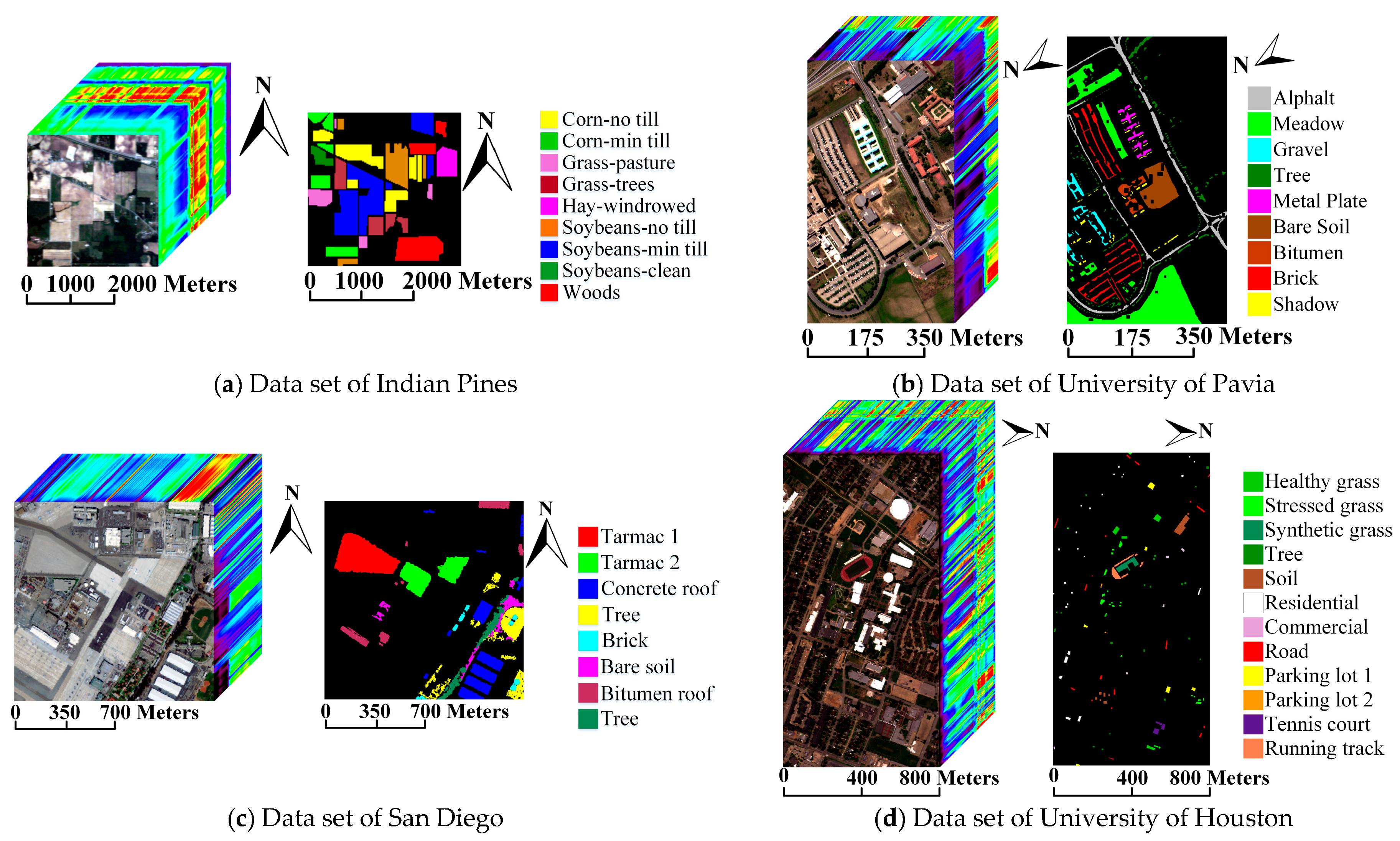
The first data set is the well-known scene taken in 1992 by the Airborne Visible Infrared Imaging Spectrometer (AVIRIS) sensor over the Indian Pines region in Northwestern Indiana. It has 144 × 144 pixels and 200 spectral bands with a pixel resolution of 20 m. Nine classes including different categories of crops have been labeled in the ground truth image.

(2)

The second data set was collected over the University of Pavia, Italy, by the Reflective Optics System Imaging Spectrometer (ROSIS) system. It consists of 103 spectral bands after removing the noisy bands, and 610 × 340 pixels for each band with a pixel resolution of 1.3 m. The ground truth image contains nine classes [37,38].

(3)

The third data set is a low-altitude AVIRIS HS image of a portion of the North Island of the U.S. Naval Air Station in San Diego, CA, USA. This HS image consists of 126 bands of size 400 × 400 pixels with a spatial resolution of 3.5 m per pixel after removing the noisy bands. The ground truth image has eight classes inside [39].

(4)

The last data set is provided by the 2013 Institute of Electrical and Electronics Engineers (IEEE) Geoscience and Remote Sensing Society (GRSS) Data Fusion Contest (DFC). It was acquired by the compact airborne spectrographic imager sensor (CASI) over the University of Houston campus and neighboring urban area, and consists of 144 bands with a spatial resolution of 2.5 m. A subset of size 640 × 320 is used, which contains 12 classes in the corresponding ground truth image. Figure 1 shows the experimental data sets.

2.2. Weighted Semi-Supervised Local Discriminant Analysis

Semi-supervised local discriminant analysis is a semi-supervised feature extraction method that has been applied in hyperspectral image classification. It combines the supervised FE method-local Fisher discriminant analysis and unsupervised FE method-neighborhood preserving embedding, and thus attempts to discover the local discriminative information of the data while preserving the local neighbor information [36]. Compared with other typical semi-supervised FE methods, SLDA focuses more on the exploration of local information, and gives a more accurate description of the distribution of samples. For better illustration, we first briefly review the feature extraction methods.

Let $x_i\in {ℝ}^d$ be a $d$-dimensional sample vector, and $\mathit{X}={\left\{x_i\right\}}_{i=1}^n$ be the matrix of $n$ samples. $\mathit{Z}={\mathit{T}}^{\mathcal{T}}X,\left(\mathit{Z}\in {ℝ}^{r\times n}\right)$ is the low-dimensional representation of the sample matrix, where $\mathit{T}\in {ℝ}^{d\times r}$ is the transformation matrix, $\mathcal{T}$ denotes the transpose.

Many dimensionality reduction techniques developed so far involve an optimization problem of the following form [40]:

$$\mathit{T}=\arg \underset{\mathit{T}}{\max }\left[\frac{\left|{\mathit{T}}^{\mathcal{T}}{\mathit{S}}^b\mathit{T}\right|}{\left|{\mathit{T}}^{\mathcal{T}}{\mathit{S}}^w\mathit{T}\right|}\right]$$

(1)

Generally speaking, ${\mathit{S}}^b$ (and ${\mathit{S}}^w$) corresponds to the quantity that we want to increase (and decrease), for example, between-class scatter (and within-class scatter). Equation (1) is equal to the solution of the following generalized eigenvalue problem:

$${\mathit{S}}^b\mathsf{\phi }=\mathsf{\lambda }{\mathit{S}}^w\mathsf{\phi }$$

(2)

where ${\left\{{\phi }_k\right\}}_{k=1}^d$ is the generalized eigenvectors associated with the generalized eigenvalues ${\left\{{\lambda }_k\right\}}_{k=1}^d ,\left({\lambda }_1>{\lambda }_2>\dots >{\lambda }_d\right).$ $\mathit{T}={\left\{{\phi }_k\right\}}_{k=1}^r$ is composed of the first $r$ eigenvectors corresponding to the largest eigenvalues ${\left\{{\lambda }_k\right\}}_{k=1}^r$. Particularly, when ${\mathit{S}}^b$ is the total scatter matrix of all samples, and ${\mathit{S}}^w={\mathit{I}}_{d\times d}$, where $\mathit{I}$ denotes the identity matrix. Equation (1) turns into the PCA method.

2.2.1. Local Fisher Discriminant Analysis (LFDA)

Suppose $y_i=c$, $c\in \left\{1,2,\dots , C\right\}$ is the associated class labels of the sample vector $x_i$. $C$ is the number of classes. $n_c$ is the number of samples in class $c$, then $\sum _{c=1}^C{n}_c=n$. Let ${\mathit{S}}^b$ and ${\mathit{S}}^w$ be the local between-class and within-class scatter matrices, respectively, defined by [41],

$$\begin{array}{c}{\mathit{S}}^b=\frac{1}{2}{\displaystyle {\displaystyle \sum }_{i=1}^n{\displaystyle \sum }_{j=1}^n}{\mathit{W}}_{i,j}^b\left(x_i-x_j\right){\left(x_i-x_j\right)}^{\mathcal{T}}\\ {\mathit{S}}^w=\frac{1}{2}{\displaystyle {\displaystyle \sum }_{i=1}^n{\displaystyle \sum }_{j=1}^n}{\mathit{W}}_{i,j}^w\left(x_i-x_j\right){\left(x_i-x_j\right)}^{\mathcal{T}}\end{array}$$

(3)

then Equation (2) turns into a local Fisher discriminant analysis problem, where ${\mathit{W}}^b$ and ${\mathit{W}}^w$ are $n\times n$ matrices,

$$\begin{array}{l}{\mathit{W}}_{\mathit{i},\mathit{j}}^{\mathit{b}}=\{\begin{array}{l}{\mathit{A}}_{i,j}\left(1/n-1/n_c\right),if y_i=y_j=c\hfill \\ 1/n, if y_i\ne y_j\hfill \end{array} \hfill \\ {\mathit{W}}_{i,j}^w=\{\begin{array}{l}{\mathit{A}}_{i,j}/n_c,if{y}_i=y_j=c\hfill \\ 0,if{y}_i\ne y_j\hfill \end{array}\hfill \end{array}$$

(4)

$A_{i,j}$ is the affinity value between $x_i$ and $x_j$. $A_{i,j}$ is large if the two samples are close, and vice versa. The definition of $A_{i,j}$ can be found in [42]. Note that we do not weight the values for the sample pairs in different classes. If $\forall i,j,{\mathit{A}}_{i,j}=1$, then LFDA degenerates into the classical Fisher discriminant analysis (FDA or linear discriminant analysis, LDA) [43]. Thus, LFDA can be regarded as a localized variant of FDA, which overcomes the weakness of LDA against within-class multimodality or outliers.

2.2.2. Neighborhood Preserving Embedding (NPE)

NPE is an unsupervised feature extraction method that seeks a projection that preserves neighboring data structure in the low-dimensional feature space [44]. It can characterize the local structural information of massive unlabeled samples. The first step of NPE is also to construct an adjacency graph, and then compute the weight matrix $\mathit{Q}$ by solving the following objective function,

$$\begin{array}{c}\min {\displaystyle {\displaystyle \sum }_i}{\displaystyle \Vert }{x}_i-{\displaystyle {\displaystyle \sum }_j}{\mathit{Q}}_{ij}{x}_j{{\displaystyle \Vert }}^2\\ s.t.{\displaystyle {\displaystyle \sum }_j}{\mathit{Q}}_{ij}=1\end{array}$$

(5)

In other words, for each sample, we use its K-nearest neighbors (KNN) to reconstruct it. Thus, the goal of NPE is to preserve this neighbor relationship in the projected low-dimensional space,

$$\begin{array}{c}\min {\displaystyle {\displaystyle \sum }_i}{\displaystyle \Vert }{z}_i-{\displaystyle {\displaystyle \sum }_j}{\mathit{Q}}_{ij}{z}_j{{\displaystyle \Vert }}^2\\ s.t.{\displaystyle {\displaystyle \sum }_j}{\mathit{Q}}_{ij}=1\end{array}$$

(6)

where $z_i={\mathit{T}}^{\mathcal{T}}{x}_i$. Then we have

$$\min trace\left[\mathit{Z}{\left(\mathit{I}-\mathit{Q}\right)}^{\mathcal{T}}\left(\mathit{I}-\mathit{Q}\right){\mathit{Z}}^{\mathcal{T}}\right]$$

(7)

By imposing the following constraint,

$${\displaystyle \sum }_i{z}_i{z}_i^{\mathcal{T}}=\mathit{I}⟹\mathit{Z}{\mathit{Z}}^{\mathcal{T}}=\mathit{I}.$$

(8)

the transformation matrix can be optimized by solving the following generalized eigenvalue problem,

$$\mathit{X}{\mathit{X}}^{\mathcal{T}}\phi =\lambda \mathit{X}\mathit{M}{\mathit{X}}^{\mathcal{T}}\phi$$

(9)

where $\phi$ denotes generalized eigenvectors, and $\mathit{M}={\left(\mathit{I}-\mathit{Q}\right)}^{\mathcal{T}}\left(\mathit{I}-\mathit{Q}\right)$.

2.2.3. Weighted SLDA

It has been demonstrated that the performance of LFDA (and all other supervised dimensionality reduction methods) tends to degrade if only a small number of labeled samples are available [40], while PCA or NPE (and other unsupervised feature extraction (FE) methods) will generally lose the discriminative information of labeled information. Thus, combining supervised and unsupervised FE methods [45] is believed to compensate for each other’s weaknesses. In this paper, we consider the combination of the aforementioned LFDA and NPE methods. As mentioned above, feature extraction techniques can be transformed into eigenvalue problems, thus, a possible way to combine LFDA and NPE is to merge the above generalized eigenvalue problems as follows [40],

$$\begin{array}{c}\begin{array}{c}\beta {\mathit{S}}^b\phi =\lambda \beta {\mathit{S}}^w\phi \\ \left(1-\beta \right)\mathit{X}{\mathit{X}}^{\mathcal{T}}\phi =\lambda \left(1-\beta \right)\mathit{X}\mathit{M}{\mathit{X}}^{\mathcal{T}}\phi \end{array}\\ \Downarrow \\ \begin{array}{c}\left[\beta {\mathit{S}}^b+\left(1-\beta \right)\mathit{X}{\mathit{X}}^{\mathcal{T}}\right]\phi \\ =\lambda \left[\beta {\mathit{S}}^w+\left(1-\beta \right)\mathit{X}\mathit{M}{\mathit{X}}^{\mathcal{T}}\right]\phi \end{array}\end{array}$$

(10)

where $\beta \in \left[0,1\right]$ is a trade-off parameter. Calculating the ${\mathit{S}}^b$ and ${\mathit{S}}^w$ of LFDA is time-consuming; an efficient implementation can be used according to [41]. Let ${\mathit{S}}^m$ denote the local mixture scatter matrix,

$${\mathit{S}}^m={\mathit{S}}^b+{\mathit{S}}^w=\frac{1}{2}{\displaystyle \sum }_{i=1}^n{\displaystyle \sum }_{j=1}^n{\mathit{W}}_{i,j}^m\left(x_i-x_j\right){\left(x_i-x_j\right)}^{\mathcal{T}}$$

(11)

where

$${\mathit{W}}^m={\mathit{W}}^b+{\mathit{W}}^w=\{\begin{array}{l}{\mathit{A}}_{i,j}/n,if{y}_i=y_j\hfill \\ 1/n,if{y}_i\ne y_j\hfill \end{array}$$

(12)

Since Equation (3) can be expressed as

$$\begin{array}{l}{\mathit{S}}^w={\displaystyle {\displaystyle \sum }_{i=1}^n{\displaystyle \sum }_{j=1}^n}{\mathit{W}}_{i,j}^w{x}_i{x}_i^{\mathcal{T}}-{\displaystyle {\displaystyle \sum }_{i=1}^n{\displaystyle \sum }_{j=1}^n}{\mathit{W}}_{i,j}^w{x}_i{x}_j^{\mathcal{T}}\hfill \\ =\mathit{X}\left({\mathit{D}}^w-{\mathit{W}}^w\right){\mathit{X}}^{\mathcal{T}}\hfill \end{array}$$

(13)

where ${\mathit{D}}^w$ is the $n$-dimensional diagonal matrix with ${\mathit{D}}_{i,i}^w={\sum }_{j=1}^n{\mathit{W}}_{i,j}^w$. Similarly, ${\mathit{S}}^m$ can be expressed as

$${\mathit{S}}^m=\mathit{X}\left({\mathit{D}}^m-{\mathit{W}}^m\right){\mathit{X}}^{\mathcal{T}}$$

(14)

where ${\mathit{D}}^m$ is the $n$-dimensional diagonal matrix with ${\mathit{D}}_{i,i}^m={\sum }_{j=1}^n{\mathit{W}}_{i,j}^m$. Therefore, the generalized eigenvalue problem of LFDA, namely Equation (2), can be rewritten as

$$\mathit{X}{\mathit{L}}^{\mathit{b}}{\mathit{X}}^{\mathcal{T}}\phi =\lambda \mathit{X}{\mathit{L}}^w{\mathit{X}}^{\mathcal{T}}\phi$$

(15)

where ${\mathit{L}}^w={\mathit{D}}^w-{\mathit{W}}^w$, ${\mathit{L}}^{\mathit{b}}=\left({\mathit{D}}^m-{\mathit{W}}^m\right)-\left({\mathit{D}}^w-{\mathit{W}}^w\right)$, from which we can see that the eigenvalue problem of LFDA has a similar form with NPE, i.e., Equation (9).

Suppose the training sample vectors are arranged by $\mathit{X}=\left[{\mathit{X}}^L,{\mathit{X}}^U\right]$, where ${\mathit{X}}^L={\left\{x_i^L\right\}}_{i=1}^{n_l}$ denotes the labeled samples, and ${\mathit{X}}^U={\left\{x_i^U\right\}}_{i=1}^{n_u}$ denotes the unlabeled samples, where $n=n_l+n_u$ is the total number of available samples. We can define the following matrices

$$\begin{gathered} {\mathit{P}}_{\mathbf{1}}=\left[\begin{array}{cc}{\mathit{L}}^{\mathit{b}}& {\mathbf{0}}_{n_l\times n_u}\\ {\mathbf{0}}_{n_u\times n_l}& {\mathbf{0}}_{n_u\times n_l}\end{array}\right],{\mathit{P}}_{\mathbf{2}}=\left[\begin{array}{cc}{\mathit{L}}^{\mathit{w}}& {\mathbf{0}}_{n_l\times n_u}\\ {\mathbf{0}}_{n_u\times n_l}& {\mathbf{0}}_{n_u\times n_u}\end{array}\right] \\ {\mathit{P}}_{\mathbf{3}}=\left[\begin{array}{cc}{\mathbf{0}}_{n_l\times n_l}& {\mathbf{0}}_{n_l\times n_u}\\ {\mathbf{0}}_{n_u\times n_l}& I_{n_u\times n_u}\end{array}\right],{\mathit{P}}_{\mathbf{4}}=\left[\begin{array}{cc}{\mathbf{0}}_{n_l\times n_l}& {\mathbf{0}}_{n_l\times n_u}\\ {\mathbf{0}}_{n_u\times n_l}& \mathit{M}\end{array}\right] \end{gathered}$$

(16)

Therefore, the weighted SLDA is equal to the solution of the following generalized eigenvalue problem

$$\begin{array}{c}\begin{array}{c}\beta \mathit{X}{\mathit{P}}_{\mathbf{1}}{\mathit{X}}^{\mathcal{T}}\phi =\lambda \beta \mathit{X}{\mathit{P}}_{\mathbf{2}}{\mathit{X}}^{\mathcal{T}}\phi \\ \left(1-\beta \right)\mathit{X}{\mathit{P}}_{\mathbf{3}}{\mathit{X}}^{\mathcal{T}}\phi =\lambda \left(1-\beta \right)\mathit{X}{\mathit{P}}_{\mathbf{4}}{\mathit{X}}^{\mathcal{T}}\phi \end{array}\\ \Downarrow \\ \begin{array}{c}{\mathit{S}}^{rb}=\mathit{X}\left[\beta {\mathit{P}}_{\mathbf{1}}+\left(1-\beta \right){\mathit{P}}_{\mathbf{3}}\right]{\mathit{X}}^{\mathcal{T}}\\ {\mathit{S}}^{rw}=\mathit{X}\left[\beta {\mathit{P}}_{\mathbf{2}}+\left(1-\beta \right){\mathit{P}}_{\mathbf{4}}\right]{\mathit{X}}^{\mathcal{T}}\\ \Downarrow \\ {\mathit{S}}^{rb}\phi =\lambda {\mathit{S}}^{rw}\phi \end{array}\end{array}$$

(17)

and $\beta$ is the trade-off parameter. In general, $0<\beta <1$ inherits the characteristics of both LFDA and NPE, and thus makes full use of both the class discriminative and local neighbor spatial information. In practice, searching for the optimal $\beta$ is time-consuming and sometimes impractical if there are insufficient labeled samples available for validation. Several research studies suggest that ensemble learning methods can be employed to avoid the huge effort of searching for the optimal parameters [46,47]. On the other hand, different parameters also lead to diversity among features or classifiers, which benefits the generalization performance of the ensembles. Hence, we present an EL method based on the idea of RoF and the weighted SLDA algorithm.

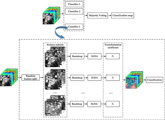
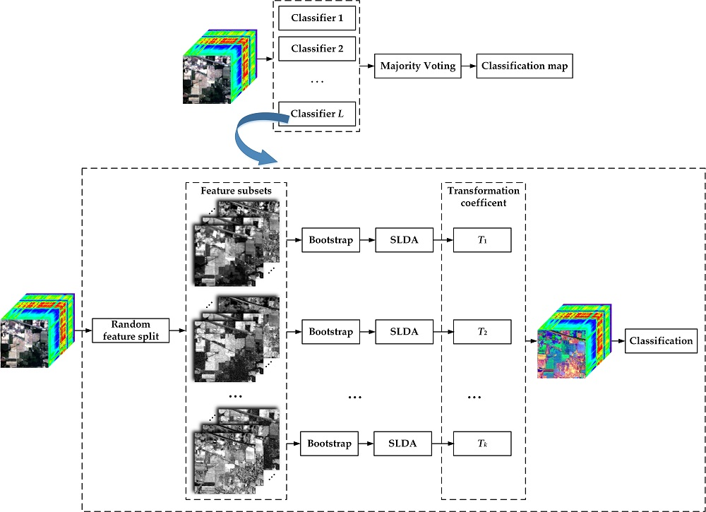
2.3. Proposed Semi-Supervised Rotation Forest

Rotation forest was developed from conventional random forest to building independent decision trees on different sets of features. It consists of splitting the feature set into several random disjoint subsets, running PCA separately on each subset, and reassembling the extracted features [30,48]. By applying different splits of the features, diverse classifiers are obtained. The main steps of RoF are briefly presented as follows:

• The original feature set is divided randomly into $K$ disjoint subsets with each subset containing $M$ features;
• Use the bootstrap approach to select a subset of the training samples for each feature subset (typically 75% of the total training samples);
• Run PCA on each feature subset and store the transformation coefficients;
• Reorder the coefficients to match the original features, rotate the samples using the obtained coefficients (i.e., feature extraction);
• Perform DT on the rotated training and testing samples;
• The process is repeated $L$ times to obtain multiple classifiers, followed by a majority voting rule to integrate the classification results.

By substituting SLDA for the PCA method, we propose the following SSRoF ensemble algorithm.

Apart from the different FE methods between Algorithm 1 and RoF, we use the different weights ($\beta$) to balance the discriminative information and structure information, thereby enhancing the diversity of features. Although the computation of the eigenvector matrix is repeated ten times (corresponding to different $\beta$) for each feature subset, it can be noticed that since the within-class and between-class scatter matrices are invariant for different weights, the computation cost is greatly reduced. Of course, the discrete values of $\beta$ can be set by different steps; we recommend the values above by considering both the diversity and computation time.

Algorithm 1: Procedures of SSRoF

Input: Training samples $X^L={\left\{x_i^L\right\}}_{i=1}^{n_l}$, testing samples $X^T={\left\{x_i^T\right\}}_{i=1}^{n_l}$, unlabeled samples $X^U={\left\{x_i^U\right\}}_{i=1}^{n_u}$, ensemble classifiers $L$, number of feature subsets $K$, ensemble $ℒ=\varnothing$ Output: Class labels of $X^T$ For $i=1:L$ 1. Randomly split the features into $K$ subsets; For $j=1:K$ 2.  Randomly select a subset of samples from $X^L$ and $X^U$, respectively, (typically 75% of samples) using bootstrap approach; 3.  Perform the weighted SLDA algorithm by the subset of $X^L$ and $X^U$ to obtain the pairs of between-class and within-class scatter matrices in Equation (17);  For $\beta =0.1:0.1:1$ 4.   Obtain the eigenvector matrix $T_{j,\beta }$ by solving Equation (17);  End for End for For $\beta =0.1:0.1:1$ 5.  Construct the transformation matrix $T_{\beta }=\left[T_{1,\beta },T_{2,\beta },\dots ,T_{K,\beta }\right]$ by merging the eigenvector matrices, and rearrange the columns of $T_{\beta }$ to match the order of original features; 6.  Build DT sub-classifier using $T_{\beta }^{\mathcal{T}}{X}^L$; 7. Perform classification for $T_{\beta }^{\mathcal{T}}{X}^T$ by using the sub-classifier; End for End for 8. Use a majority voting rule for the $L\times 10$ sub-classifiers to compute the confidence of $X^T$ and assign a class label for each testing sample;

3. Experimental Results and Discussion

In this section, we report the experiments on the four groups of hyperspectral images. First, the presented method is compared with several other EL algorithms to show the advantages. Then, we also introduce the performance evaluation of our method under different parameters.

3.1. Experimental Setup

In order to demonstrate the advantages of the proposed algorithm, we conducted the experiments under different numbers of training samples, and compared with several state-of-the-art ensemble learning methods, namely random forest (RF), semi-supervised feature extraction combined RF ensemble method (SSFE-RF) [22], rotation forest (RoF) [30], and rotation random forest-KPCA (RoRF-KPCA) [32]. For better comparison, the SLDA method was also used as a preprocessing step that combined with the original RoF method (we refer to it as SLDA-RoF). Finally, the LFDA and NPE methods were also used as rotation means like RoF method.

The numbers of trees were all set to $L=10$, and the classification and regression tree (CART) was adopted as the base classifier. The numbers of features in each subset were all set to $M=10$ for SSFE-RF, RoF, RoF-LFDA, RoF-NPE, and SSRoF. For RoRF-KPCA, Xia et al. [32] suggest that a small number of features per subset will increase the classification performance, as such, we set $M=5$. For RF, the number of features considered at each node was set as the square root of the used feature number. The numbers of extracted features were set equal to $M$ for RoF, RoRF-KPCA, RoF-LFDA, RoF-NPE, and SSRoF. For SLDA, the number of extracted features was set to half of the original features, and other parameters were set to the same as RoF. For RoRF-KPCA, it is quite difficult to select the optimal kernel parameters. Xia et al. [32] declares that parameter tuning is needed, but different kernel functions (linear, radial basis function, and Polynomial) provide very similar results, making this choice not critical in this context. Considering the performance enhancement and the computation cost, in our experiments, we use the polynomial kernels with the degree equals to two.

The performance is evaluated by the overall accuracy (OA), and Kappa coefficient. In all cases, we conduct ten independent Monte Carlo runs with respect to the labeled training set from the ground truth images. And the results are the average values of the 10 runs. The numbers of available samples are listed in

Table 1. Number of available samples in each data set.

Indian Pines		University of Pavia		San Diego		University of Houston
Class	Samples	Class	Samples	Class	Samples	Class	Samples
corn-no till	1434	asphalt	6304	tarmac1	7044	healthy grass	449
corn-min till	834	meadow	18146	tramac2	4721	stressed grass	454
grass-pasture	234	gravel	1815	concrete roof	5771	synthetic grass	505
grass-trees	497	tree	2912	tree	4851	tree	293
hay-windrowed	747	metal plate	1113	brick	873	soil	688
soybeans-no till	489	bare soil	4572	bare soil	1748	residential	26
soybeans-min till	968	bitumen	981	bitumen roof	2454	commercial	463
soybeans-clean	2468	brick	3364	tree	2135	road	112
woods	1294	shadow	795			parking lot 1	427
						parking lot 2	247
						tennis court	473
						running track	367

.

3.2. Performance Evaluation

The comparison of different EL algorithms is presented here. We randomly selected 1%, 2%, and 5% samples of each class as training samples for the first three data sets, and 5%, 10%, and 20% for the last data set. The remaining samples were used for testing purposes.

Table 2. The overall accuracies (%) and Kappa coefficients of different algorithms.

		RF	SSFE-RF	RoF	RoRF-KPCA	SLDA-RoF	RoF-LFDA	RoF-NPE	SSRoF
Indian	1%	58.35 0.5018	66.87 0.5995	71.48 0.6587	70.54 0.6491	63.88 0.5660	66.17 0.5943	69.39 0.6337	74.38 0.6918
	2%	64.55 0.5746	74.89 0.6971	75.80 0.7117	77.11 0.7272	70.22 0.6437	76.72 0.7214	76.45 0.7179	80.83 0.7710
	5%	70.79 0.6502	81.04 0.7728	82.97 0.7971	82.96 0.7971	77.58 0.7330	83.01 0.7978	82.66 0.7936	86.84 0.8429
Pavia	1%	79.65 0.7143	84.93 0.7879	87.13 0.8223	87.02 0.8205	81.20 0.7373	87.09 0.8214	86.67 0.8152	88.98 0.8484
	2%	82.38 0.7538	87.27 0.8220	89.54 0.8559	89.39 0.8537	84.34 0.7840	90.15 0.8645	89.61 0.8571	91.60 0.8846
	5%	85.82 0.8029	90.26 0.8648	92.28 0.8943	92.10 0.8919	86.82 0.8186	92.52 0.8978	91.77 0.8871	93.67 0.9137
San Diego	1%	86.08 0.8333	96.07 0.9529	95.28 0.9435	94.19 0.9305	93.25 0.9192	95.20 0.9426	95.55 0.9467	95.99 0.9520
	2%	90.10 0.8814	96.78 0.9615	96.40 0.9569	95.88 0.9507	94.86 0.9385	96.50 0.9582	96.56 0.9589	97.02 0.9644
	5%	93.10 0.9175	97.69 0.9724	97.64 0.9717	97.09 0.9652	96.40 0.9569	97.62 0.9716	97.61 0.9715	98.02 0.9764
Houston	5%	91.32 0.9034	95.97 0.9551	96.06 0.9561	96.08 0.9564	93.73 0.9302	96.06 0.9561	96.33 0.9591	97.43 0.9714
	10%	94.40 0.9376	96.59 0.9620	97.08 0.9676	97.60 0.9733	94.98 0.9441	96.96 0.9662	97.33 0.9703	98.09 0.9787
	20%	96.31 0.9590	98.03 0.9780	98.18 0.9798	98.42 0.9824	96.54 0.9615	98.22 0.9802	97.77 0.9752	98.60 0.9845

RF: random forest; SSFE-RF: semi-supervised feature extraction combined random forest; RoF: rotation forest; RoRF-KPCA: rotation random forest with kernel principal component analysis; SLDA-RoF: RoF with semi-supervised local discriminant analysis pre-processing; RoF with local Fisher discriminant analysis; RoF-NPE: RoF with neighborhood preserving embedding; SSRoF: semi-supervised rotation forest.

lists the classification results of the four algorithms under different numbers of samples. The upper line in each cell denotes the overall accuracies, and the lower line is the Kappa values. For clarity, the best results are shown in different colors.

From the table, it can be seen obviously that all the other methods yielded much higher accuracies than the conventional RF method. SSFE-RF achieved higher accuracies than RF due to the increment in the number of classifiers and the semi-supervised feature extraction method. Particularly, it had splendid performance on the San Diego data set. Moreover, except for the SLDA-RoF, all of the other RoF-based approaches also surpassed the RF-based methods in most cases, which demonstrates the promotion of diversity owing to the random feature extraction. RoRF-KPCA yielded similar results with RoF, although it considers the nonlinear characteristics of hyperspectral data, and would have constructed reliable rotation matrices to generate high precision classification results. A probable reason may be the selection of sub-optimal parameters for kernel functions. However, as we have mentioned, searching for the optimal parameters remains problematic, and RoRF-KPCA is not sensitive to the changes of the kernel function. A smaller value of $M$ may also affect the classification accuracy, although a smaller $M$ means a larger $K$, which leads to a higher computational complexity due to the construction of the kernel matrix. Regardless of the computation time, it can be expected that RoRF-KPCA can surpass RoF to some extent. It can also be seen that RoF-LFDA and RoF-NPE also produced similar results as RoF. RoF-LFDA sometimes performed better than RoF and RoF-NPE when more samples were available, since it only uses the discriminative information of the labeled samples. In fact, no matter which simple rotation method was used in RoF, it seems that the results were very close to each other on the whole. However, the SLDA combined RoF method has relatively lower accuracies compared with other RoF-based method, although it has been demonstrated to perform well for other conventional classifiers [36] (e.g., MLC, SVM). Thus, it seems to be not suitable for rotation forest algorithms.

By contrast, the proposed SSRoF outperformed the others clearly in most cases from both OA and Kappa values, especially on the Indian and Pavia data sets (4.35% and 1.45% higher than RoF for the Indian and Pavia data sets on average, respectively). Although the conventional RF and RoF-based algorithms performed well on the last data set, the proposed algorithm still showed slight superiority. The main reason why the proposed SSRoF method surpasses RoF-LFDA and RoF-NPE is that SSRoF uses a weighted form to better explore the discriminative information and structure information of the available samples, thus greatly promoting the diversity of features.

Particularly, aside from the number of ensembles $L$ and the number of features per subset ($M$), the proposed approach needs fewer additional parameters, which makes the approach much easier to implement.

3.3. Impact of Parameters

In this sub-section, we will discuss the impact of two basic parameters, i.e., the number of ensembles ($L$), and the number of features in each subset ($M$). For brevity, we simply show the results performed on the data sets of Indian Pines and University of Pavia by setting different number of trees, i.e., $L=$2, 5, 10, 20, and 30. Likewise, the experiments are conducted under different numbers of training samples. The results are shown in

Table 3. The classification results of SSRoF under different number of ensembles ($L$). OA: overall accuracy.

		$\mathit{L}=2$		$\mathit{L}=5$		$\mathit{L}=10$		$\mathit{L}=20$		$\mathit{L}=30$
		OA (%)	Kappa	OA (%)	Kappa	OA (%)	Kappa	OA (%)	Kappa	OA (%)	Kappa
Indian	1%	71.01	0.6516	74.16	0.6887	74.69	0.6955	74.65	0.6944	74.96	0.6978
	2%	77.91	0.7359	79.56	0.7545	80.03	0.7600	80.54	0.7660	80.95	0.7710
	5%	83.55	0.8039	85.63	0.8285	86.62	0.8403	86.87	0.8432	86.97	0.8443
	10%	86.51	0.8392	88.44	0.8622	88.87	0.8672	89.24	0.8716	89.26	0.8718
	20%	88.91	0.8682	90.71	0.8894	91.25	0.8958	91.67	0.9008	91.74	0.9016
Pavia	1%	87.71	0.8308	88.79	0.8456	89.13	0.8504	89.38	0.8538	89.45	0.8548
	2%	89.74	0.8592	91.20	0.8794	91.35	0.8814	91.65	0.8856	91.75	0.8869
	5%	92.13	0.8924	93.36	0.9094	93.70	0.9141	93.78	0.9151	93.86	0.9163
	10%	93.07	0.9053	94.10	0.9195	94.46	0.9245	94.59	0.9263	94.59	0.9262
	20%	94.48	0.9250	95.15	0.9341	95.31	0.9363	95.45	0.9382	95.46	0.9383

. In order to give an intuitive evaluation, OAs and Kappa values are shown in different colors.

From Table 3 we can see that, obviously, with the increment of ensemble number, the overall accuracy and Kappa coefficient grow continuously, for instance, from nearly 67% to 75% under 1% samples for the Indian Pines data set, which demonstrates the benefit of EL. An interesting factor is that when the number of trees increases to 10, the classification accuracy grows slower and tends to reach convergence. This makes our approach more promising, since we can use less ensembles to achieve a relatively stable result, thereby reducing the computational burden.

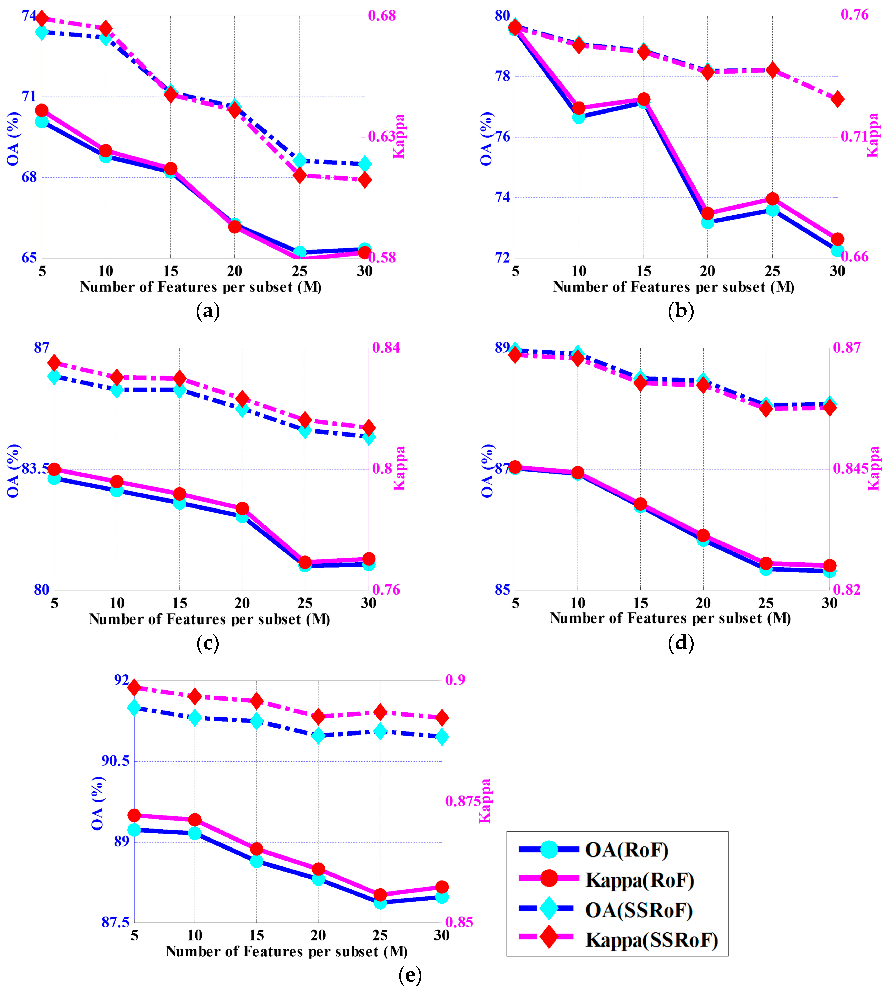
To investigate the impact of the number of features in each subset, we also performed tests on the Indian Pines data set regarding different feature divisions. For better comparison, the same process was also applied on RoF algorithm, and the results are shown in Figure 2, where the blue color denotes the OAs, and the magenta color denotes the Kappa values. The solid lines denote the RoF method, while the dot dash lines represent the SSRoF method. The figure indicates that when the number of features involved in each subset increases, i.e., the number of feature subsets ($K$) decreases, the classification results tend to degenerate for both RoF and SSRoF. In fact, this is also consistent with the conclusions of [32], and that is why we selected a small number of $M$ for the RoRF-KPCA method. Although when the training set increased, this problem seemed to be alleviated in a manner (for instance, in Figure 2e, 91.48% for $M=5$ and 90.94% for $M=30$ (SSRoF), when 20% of training samples were used), a small value of $M$ is usually preferred. However, on the other hand, a smaller M means a larger $K$, which means the rotation process will be executed more times, and this will lead to a huge computational cost. Apart from the above analysis, we can also see that the proposed approach seemed to be more stable than RoF with the increment in the number of features per subset.

4. Conclusions

Since existing rotation forest-based techniques fail to take account of the discriminative information of training samples during feature extraction, this paper proposed a semi-supervised rotation forest that uses the weighted semi-supervised local discriminant analysis method to jointly utilize the class discriminative information and local structural information provided by the labeled and unlabeled samples, respectively. The proposed algorithm aims to find the projection directions that provide better class separability, thus enhancing the performance of existing rotation forest algorithms. Furthermore, the proposed algorithm does not need additional parameters compared with the classical rotation forest method, which makes it easy to implement. Experiments have shown that the proposed algorithm outperforms several typical ensemble learning methods. Our future work will aim to reduce the computational time and assemble some other state-of-the-art machine learning algorithms.

References

- Ballanti, L.; Blesius, L.; Hines, E.; Kruse, B. Tree species classification using hyperspectral imagery: A comparison of two classifiers. Remote Sens. 2016, 8, 445. [Google Scholar] [CrossRef]
- Sami ul Haq, Q.; Tao, L.; Yang, S. Neural network based Adaboosting approach for hyperspectral data classication. In Proceedings of the 2011 International Conference on Computer Science and Network Technology (ICCSNT), Harbin, China, 24–26 December 2011. [Google Scholar]
- Melgani, F.; Bruzzone, L. Classification of hyperspectral remote sensing images with support vector machines. IEEE Trans. Geosci. Remote Sens. 2004, 42, 1778–1790. [Google Scholar] [CrossRef]
- Li, J.; Bioucas-Dias, J.; Plaza, A. Semisupervised hyperspectral image segmentation using multinomial logistic regression with active learning. IEEE Trans. Geosci. Remote Sens. 2010, 11, 4085–4098. [Google Scholar] [CrossRef]
- Persello, C.; Bruzzone, L. Active and semisupervised learning for the classification of remote sensing images. IEEE Trans. Geosci. Remote Sens. 2014, 52, 6937–6956. [Google Scholar] [CrossRef]
- Villa, A.; Chanussot, J.; Benediktsson, J.A.; Jutten, C. Spectral unmixing for the classification of hyperspectral images at a finer spatial resolution. IEEE J. Sel. Top. Signal Process. 2011, 5, 521–533. [Google Scholar] [CrossRef]
- Golipour, M.; Ghassemian, H.; Mirzapour, F. Integrating hierarchical segmentation maps with MRF prior for classification of hyperspectral images in a Bayesian framework. IEEE Trans. Geosci. Remote Sens. 2016, 54, 805–816. [Google Scholar] [CrossRef]
- Licciardi, G.; Pacifici, F.; Tuia, D.; Prasad, S.; West, T.; Giacco, F.; Thiel, C.; Inglada, J.; Christophe, E.; Chanussot, J.; et al. Decision fusion for the classification of hyperspectral data: Outcome of the 2008 GRSS data fusion contest. IEEE Trans. Geosci. Remote Sens. 2009, 47, 3857–3865. [Google Scholar] [CrossRef]
- Wozniak, M.; Graña, M.; Corchado, E. A survey of multiple classifier systems as hybrid systems. Inf. Fusion 2014, 16, 3–17. [Google Scholar] [CrossRef]
- Krawczyk, B.; Minku, L.L.; Gama, J.; Stefanowski, J.; Wozniak, M. Ensemble learning for data stream analysis: A survey. Inf. Fusion 2017, 37, 132–156. [Google Scholar] [CrossRef]
- Santos, A.B.; Araújo, A.A.; Menotti, D. Combining multiple classification methods for hyperspectral data interpretation. IEEE J. Sel. Top. Appl. Earth Obs. Remote Sens. 2013, 6, 1450–1459. [Google Scholar] [CrossRef]
- Waske, B.; Linden, S.V.D.; Benediktsson, J.A.; Rabe, A.; Hostert, P. Sensitivity of support vector machines to random feature selection in classification of hyperspectral data. IEEE Trans. Geosci. Remote Sens. 2010, 2880–2889. [Google Scholar] [CrossRef]
- Wang, S.; Yao, X. Relationships between diversity of classification ensembles and single-class performance measures. IEEE Trans. Knowl. Data Eng. 2013, 25, 206–219. [Google Scholar] [CrossRef]
- Galar, M.; Fernandez, A.; Barrenechea, E.; Bustince, H.; Herrera, F. A review on ensembles for the class imbalance problem: Bagging-, Boosting-, and hybrid-based approaches. IEEE Trans. Syst. Man Cybern.—Part C: Appl. Rev. 2012, 42, 463–484. [Google Scholar] [CrossRef]
- Friedman, J.H. Greedy function approximation: A gradient boosting machine. Ann. Stat. 2001, 29, 1189–1232. [Google Scholar] [CrossRef]
- Breiman, L. Bagging predictors. Mach. Learn. 1996, 24, 123–140. [Google Scholar] [CrossRef]
- Schapire, R.E. The strength of weak learn ability. Mach. Learn. 1990, 5, 197–227. [Google Scholar] [CrossRef]
- Schapire, R.E.; Singer, Y. Improved boosting algorithms using confidence-rated predictions. Mach. Learn. 1999, 37. [Google Scholar] [CrossRef]
- Ho, T.K. The random subspace method for constructing decision forests. IEEE Trans. Pattern. Anal. Mach. Intell. 1998, 20, 832–844. [Google Scholar] [CrossRef]
- Breiman, L. Random forests. Mach. Learn. 2001, 45, 5–32. [Google Scholar] [CrossRef]
- Ham, J.; Chen, Y.; Crawford, M.M.; Ghosh, J. Investigation of the random forest framework for classification of hyperspectral data. IEEE Trans. Geosci. Remote Sens. 2005, 43, 492–501. [Google Scholar] [CrossRef]
- Xia, J.; Liao, W.; Chanussot, J.; Du, P.; Song, G.; Philips, W. Improving random forest with ensemble of features and semisupervised feature extraction. IEEE Geosci. Remote Sens. Lett. 2015, 12, 1471–1475. [Google Scholar] [CrossRef]
- Chan, J.C.; Paelinckx, D. Evaluation of random forest and Adaboost tree-based ensemble classification and spectral band selection for ecotope mapping using airborne hyperspectral imagery. Remote Sens. Environ. 2008, 112, 2999–3011. [Google Scholar] [CrossRef]
- Rodriguez-Galianoa, V.F.; Ghimireb, B.; Roganb, J.; Chica-Olmoa, M.; Rigol-Sanchezc, J.P. An assessment of the effectiveness of a random forest classifier for land-cover classification. ISPRS J. Photogramm. Remote Sens. 2012, 67, 93–104. [Google Scholar] [CrossRef]
- Merentitis, A.; Debes, C.; Heremans, R. Ensemble learning in hyperspectral image classification: Toward selecting a favorable bias-variance tradeoff. IEEE J. Sel. Top. Appl. Earth Obs. Remote Sens. 2014, 7, 1089–1102. [Google Scholar] [CrossRef]
- Gurram, P.; Kwon, H. Sparse kernel-based ensemble learning with fully optimized kernel parameters for hyperspectral classification problems. IEEE Trans. Geosci. Remote Sens. 2013, 51, 787–802. [Google Scholar] [CrossRef]
- Samat, A.; Du, P.; Liu, S.; Li, J.; Cheng, L. E2LMs: Ensemble extreme learning machines for hyperspectral image classification. IEEE J. Sel. Top. Appl. Earth Obs. Remote Sens. 2014, 7, 1060–1069. [Google Scholar] [CrossRef]
- Guo, H.; Li, Y.; Jennifer, S.; Gu, M.; Huang, Y.; Gong, B. Learning from class-imbalanced data: Review of methods and applications. Expert Syst. Appl. 2017, 73, 220–239. [Google Scholar] [CrossRef]
- Merentitis, A.; Debes, C. Many hands make light work-on ensemble learning techniques for data fusion in remote sensing. IEEE Geosci. Remote Sens. Mag. 2015, 3, 86–99. [Google Scholar] [CrossRef]
- Rodriguez, J.J.; Kuncheva, L.I. Rotation forest: A new classifier ensemble method. IEEE Trans. Pattern Anal. Mach. Intell. 2006, 28, 1619–1630. [Google Scholar] [CrossRef] [PubMed]
- Ayerdi, B.; Romay, M.G. Hyperspectral image analysis by spectral-spatial processing and anticipative hybrid extreme rotation forest classification. IEEE Trans. Geosci. Remote Sens. 2016, 54, 2627–2639. [Google Scholar] [CrossRef]
- Xia, J.; Falco, N.; Benediktsson, J.A.; Du, P.; Chanussot, J. Hyperspectral image classification with rotation random forest via KPCA. IEEE J. Sel. Top. Appl. Earth Obs. Remote Sens. 2017, 10, 1601–1609. [Google Scholar] [CrossRef]
- Chen, J.; Xia, J.; Du, P.; Chanussot, J. Combining rotation forest and multiscale segmentation for the classification of hyperspectral data. IEEE J. Sel. Top. Appl. Earth Obs. Remote Sens. 2016, 9, 4060–4072. [Google Scholar] [CrossRef]
- Rahulamathavan, Y.; Phan, R.C.-W.; Chambers, J.A.; Parish, J.D. Facial expression recognition in the encrypted domain based on local Fisher discriminant analysis. IEEE Trans. Affect. Comput. 2013, 4, 83–92. [Google Scholar] [CrossRef]
- Belhumeur, P.N.; Hespanha, J.P.; Kriegman, D.J. Eigenfaces vs. Fisherfaces: Recognition using class specific linear projection. IEEE Trans. Pattern Anal. Mach. Intell. 1997, 19, 711–720. [Google Scholar] [CrossRef]
- Lu, X.; Zhang, J.; Li, T.; Zhang, G. Synergetic classification of long-wave infrared hyperspectral and visible images. IEEE J. Sel. Top. Appl. Earth Obs. Remote Sens. 2015, 8, 3546–3557. [Google Scholar] [CrossRef]
- Sun, B.; Kang, X.; Li, S.; Benediktsson, J.A. Random-walker-based collaborative learning for hyperspectral image classification. IEEE Trans. Geosci. Remote Sens. 2017, 55, 212–222. [Google Scholar] [CrossRef]
- Kang, X.; Li, S.; Benediktsson, J.A. Feature extraction of hyperspectral images with image fusion and recursive filtering. IEEE Trans. Geosci. Remote Sens. 2014, 52, 3742–3752. [Google Scholar] [CrossRef]
- Kang, X.; Zhang, X.; Li, S.; Li, K.; Li, J.; Benediktsson, J.A. Hperspectral anomaly detection with attribute and edge-preserving filters. IEEE Trans. Geosci. Remote Sens. 2017, 1–12. [Google Scholar] [CrossRef]
- Sugiyama, M.; Idé, T.; Nakajima, S.; Sese, J. Semi-supervised local Fisher discriminant analysis for dimensionality reduction. Mach. Learn. 2010, 78, 35–61. [Google Scholar] [CrossRef]
- Sugiyama, M. Dimensionality reduction of multimodal labeled data by local Fisher discriminant Analysis. J. Mach. Learn. Res. 2007, 8, 1027–1061. [Google Scholar] [CrossRef]
- He, X.; Niyogi, P. Locality preserving projections. In Advances in Neural Information Processing Systems; MIT Press: Cambridge, MA, USA, 2004; pp. 153–160. [Google Scholar]
- Martinez, M.; Kak, A.C. PCA versus LDA. IEEE Trans. Pattern Anal. Mach. Intell. 2001, 23, 228–233. [Google Scholar] [CrossRef]
- He, X.; Cai, D.; Yan, S.; Zhang, H. Neighborhood preserving embedding. In Proceedings of the Tenth IEEE International Conference on Computer Vision, Beijing, China, 17–20 October 2005; pp. 1208–1213. [Google Scholar]
- Liao, W.; Pi, Y. Feature extraction for hyperspectral images based on semi-supervised local discriminant analysis. In Proceedings of the 2011 Joint Urban Remote Sensing Event (JURSE), Munich, Germany, 11–13 April 2011; pp. 401–404. [Google Scholar]
- Bao, R.; Xia, J.; Mura, M.D.; Du, P.; Chanussot, J.; Ren, J. Combining morphological attribute profiles via an ensemble method for hyperspectral image classification. IEEE Geosci. Remote Sens. Lett. 2016, 13, 359–363. [Google Scholar] [CrossRef]
- Xia, J.; Mura, M.D.; Chanussot, J.; Du, P.; He, X. Random subspace ensembles for hyperspectral image classification with extended morphological attribute profiles. IEEE Trans. Geosci. Remote Sens. 2015, 53, 4768–4785. [Google Scholar] [CrossRef]
- Xia, J.; Du, P.; He, X.; Chanussot, J. Hyperspectral remote sensing image classification based on rotation forest. IEEE Geosci. Remote Sens. Lett. 2014, 11, 239–243. [Google Scholar] [CrossRef]
Figure 1.
Experimental hyperspectral and corresponding ground truth images.
Figure 2.
Impact of the number of features in each subset () under different numbers of training samples (1%, 2%, 5%, 10%, and 20% from (a–e), respectively).