Fast and Efficient Correction of Ground Moving Targets in a Synthetic Aperture Radar, Single-Look Complex Image


1
Nansen Environmental and Remote Sensing Center, 5006 Bergen, Norway
2
Department of Earth System Sciences, Yonsei University, Seoul 03722, South Korea
*
Author to whom correspondence should be addressed.
Remote Sens. 2017, 9(9), 926; https://doi.org/10.3390/rs9090926
Submission received: 1 August 2017
/
Revised: 18 August 2017
/
Accepted: 28 August 2017
/
Published: 6 September 2017
(This article belongs to the Special Issue Advances in SAR: Sensors, Methodologies, and Applications)
Abstract
:Ground moving targets distort normally-focused synthetic aperture radar (SAR) images. Since most high-resolution SAR data providers only offer single-look complex (SLC) data rather than raw signals to general users, they need to apply a simple and efficient residual SAR focusing to SLC data containing moving targets. This paper presents an efficient and effective SAR residual focusing method that is practically applicable to SLC data. The residual Doppler spectrum of the moving target is derived from a general SAR configuration and normal SAR focusing. The processing steps are simple and straightforward, with a limited size of the processing window, e.g., 64 × 64. Application results using simulation data and actual TerraSAR-X SLC data with a speed-controlled vehicle demonstrate the effectiveness of the method, which particularly improves the −3 dB width, integrated sidelobe ratio, and symmetry of the reconstructed signals. In particular, the azimuthal symmetry becomes seriously distorted when the target speed is higher than 8 m/s (or 28.8 km/h), and the symmetry is well recovered by the proposed method.
1. Introduction
The imaging characteristics of ground moving targets using synthetic aperture radar (SAR) have been well known since the early stages of SAR development [1,2]. Ground moving objects in SAR single-look complex (SLC) images are typically characterized by three features: target displacement in the azimuth dimension and range walking according to the range component of the ground target velocity, azimuth image blurring (mainly due to the azimuth component of velocity and the range component of acceleration), and residual Doppler centroid. While these features distort SAR images, they have been exploited as ground moving target indicators (GMTIs) to retrieve the target’s velocity [3]. Thus, the main concerns related to ground moving objects are twofold: the detection of a moving target within an SAR image, and the estimation of physical parameters such as velocity or original location. Numerous algorithms have been proposed for GMTI, and most of them are based on sensing the difference in Doppler parameters between the moving object [4,5,6,7,8] and the fixed clutter or on detection by focusing [9,10,11,12,13,14,15,16]. For more efficient detection of ground moving targets, the theory and systems for the along-track interferometry (ATI) also have been extensively researched [13,17,18,19,20,21,22,23,24,25]. Bistatic ATI SAR systems have recently gained growing popularity [26,27,28].
While the SAR imaging characteristics are exploited for the GMTI, precise focusing remains an important issue, especially as the resolution of SAR images becomes ever higher. Various focusing methods for SAR have previously been developed, but most of them are based on raw signal processing [9,12], and recently, many have involved the keystone transformation [29,30,31]. Although several SAR focusing algorithms have been developed for ground moving targets, raw signals rather than single-look complex (SLC) data are required in most cases. However, it is not practical for general users to process raw signals because the raw signal data acquired by most current high-resolution SAR systems are not provided to users, mainly because of their complexity. Thus, it is necessary for general users to apply a residual focusing to SLC data rather than the raw signals. This study proposes a simple and straightforward method of residual focusing for ground moving targets that is practically applicable to SLC data by general users. Generally, there are two types of ground moving targets: targets moving in groups such as ocean currents and waves, and isolated small but fast-moving targets such as moving ships or cars. The proposed method is particularly applicable for the latter type, based on the point-target spectrum in the 2D frequency domain. The residual Doppler phase in the normally-focused SLC data is to be elaborately formulated and discussed. This paper presents formulae related to the residual Doppler spectrum caused by ground moving targets after azimuth and range compression, and proposes a simple and straightforward method for residual focusing of SLC images based on the derived formulae. The derived residual Doppler spectrum accounts for target distortion by the asymmetry of the compressed signals as well as image blurring. For evaluation and demonstration of the performance, the algorithm is applied to simulated data and TerraSAR-X SLC data in which a speed-controlled vehicle is imaged.
The advantages of the proposed method are twofold. First, the residual focusing is based on the derived formulae of the Doppler spectrum after image formation, which implies that targets can be precisely reconstructed in terms of main-to-sidelobe ratio and symmetry. Second, the method is simple and practical because only SLC data of high-resolution SAR systems (rather than raw signal data) are normally provided to general users. A processing window for each ground moving target is relatively small (few tens of pixels) because the image is already focused. This maximizes the computational efficiency and minimizes the distortion of neighboring stationary objects. In this paper, Section 2 and Section 3 describe the derivation of the residual Doppler spectrum after azimuth and range compression and the processing tactics. Section 4 presents the application results that demonstrate the efficiency and effectiveness of the residual focusing in terms of the −3 dB width, integrated sidelobe ratio, and symmetry of the focused signals. Finally, the discussion and conclusions follow in Section 5 and Section 6, respectively.
2. Correction Formula for SAR SLC data
2.1. Phase Effects of a Moving Target in 2D Frequency Domain
The received signal from a ground point target in a monostatic SAR configuration after demodulation is as follows [32]:
where is the transmitted signal, is the slant range distance, is the carrier frequency, is the speed of light, is the length of full aperture time, and and are the range time (or fast-time) and azimuth time (or slow-time), respectively. In general the amplitude modulation is described by two-way antenna pattern; however, since our interest here is the phase component of the returned signal, the amplitude component in Equation (1) is neglected without losing generality. The point-target spectrum of a stationary ground object in the 2D frequency domain is as follows [32,33]:
where is the Fourier transform of , is the range distance at the closest approach, is the effective antenna velocity along the azimuth direction, is the full aperture bandwidth, and and are the range frequency and azimuth (or Doppler) frequency, respectively.
Let us consider a ground moving object now. Figure 1 shows an imaging geometry of SAR to a ground object with a Cartesian coordinate . , , and axes are with the azimuth direction, the zero-Doppler ground range direction, and the normal to the earth at the antenna position, respectively. For a space-borne imaging scenario, the use of earth ellipsoid model is more appropriate. However for describing the time-varying distance of a moving object during short observation time (less than 1 second for the stripmap mode), the real imaging geometry can be approximated by plane-earth geometry. The time-varying distance, , from a ground target located in at to the antenna, changing with a velocity of and an acceleration of , is given as follows:
where , , , is the wavelength, is the altitude of antenna, and in the given imaging geometry. Thus, the returned signal from a ground moving target in signal space is
The point target spectrum in the range frequency-azimuth time domain is given by
The range walk due to the moving target is expressed by the last phase component in Equation (5) and a modification of the relative antenna velocity, , in of the first phase component, which in turn affects the Doppler slope. Then, the moving target in the 2D frequency domain can be obtained from Equation (2) by replacing the Doppler frequency, , with and the effective velocity, , with :
where
Applying Taylor expansion of by up to second order results in a simplified form as follows:
where . Compared with the stationary target case in Equation (2), the terms with and that are involved distort the point target spectrum of a ground moving target. It is necessary to compensate these terms when fine-tuning the SAR image of each ground moving target.
2.2. The Residual Phase Removal in the SAR SLC Image
Since the SAR SLC image, rather than raw signals, is usually provided to general users, it is practical to consider phase compensation in SLC data. The SAR SLC data is formed by a series of processing steps, including range-curvature-migration correction (RCMC), azimuth compression, and the secondary range compression. These three processing steps for a point target can be modeled as multiplication by the complex conjugate of the following function [33]:
where . The first term represents the transfer function of the azimuth chirp, the second that of the RCMC, and the last that of the secondary range compression [33,34]. Then, the compressed point target spectrum after compensating Equation (9) from Equation (6) in the 2D point target spectrum is given by
where
when the high-order terms are neglected. The first residual phase, , stands for the residual azimuth chirp,
The second residual phase, , is for the range shift and a coupling between the two frequencies, and ,
Finally, the third residual phase, , is for the residual range compression that is usually very small unless the target’s velocity is very high:
Among the three residual phases in Equations (12)–(14), the second term, , is the most complicated and has not been well reviewed while the first term, , has the biggest effect. in Equation (13) is composed of two terms: a slight range-time shift due to as in Equation (3) and a coupling term between Doppler frequency, , and range frequency, .
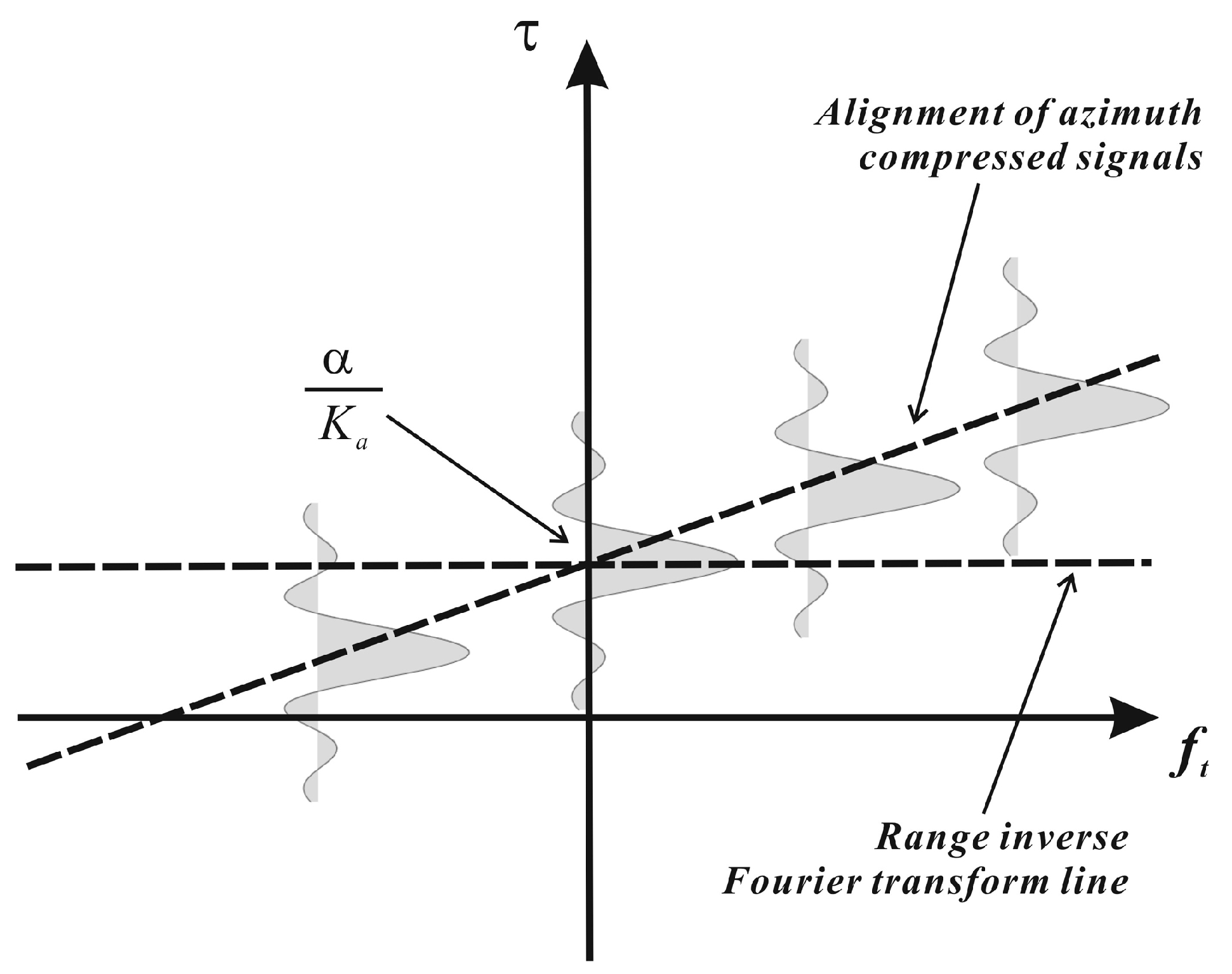
The effect of the latter is particularly significant. The coupling between the two frequencies in Equation (13) projects the azimuth-compressed signals on a slanted line rather than a horizontal line in the range frequency-azimuth time domain, as shown in Figure 2.
The inverse Fourier transform along the horizontal range frequency results in asymmetric compressed signals in both the azimuth and range dimensions, as well as dispersion of the signal power to some extent. The steeper the slope is, the more serious the distortion of the compressed signal is. The slope largely depends on (or ); consequently, the ground object with large range speed suffers a significant distortion. After removal of the three residual phases, the refocused 2D point target spectrum in Equation (10) becomes as follows:
where , which is called the Doppler slope. The point target spectrum in the range frequency-azimuth time domain after inverse Fourier transformation of the Doppler frequency is given by
It is necessary to remove the last term in the range frequency-azimuth time domain by multiplying with the complex conjugate of following term:
This process can also be achieved by applying the Keystone transform [35,36,37]. This transform is very effective if applied to raw or range-compressed signals [29,30,31,38], but this process is not a computationally efficient method. Instead of raw signals, here we consider the SLC data with which both azimuth and range compression are already performed, and unlike the rectangular function in Equation (1), the extension of the sinc function in the azimuth dimension in Equation (16) is very limited. Thus, the simple multiplication of Equation (17) would be sufficient to remove the coupling of the azimuth and range frequencies in the SLC data. After inverse-Fourier transformation () of the range frequency, the fine-tuned SLC image finally becomes as follows:
Now, the resulting effect of a ground moving target is an azimuthal shift by and a linear phase of in the fine-tuned SLC image. Recall that is a function of the range velocity of the target, the incidence angle, and the wavelength.
3. Residual Focusing of SAR SLC Data
A fine-tuning of the not fully focused ground moving targets in an SLC image can be achieved by removing the three phases in Equations (12)–(14) in the 2D frequency domain, followed by applying Equation (17) in the range frequency-azimuth time domain. Since the detection of moving targets is beyond the scope of this paper, detection tactics are not discussed herein. To apply the residual focusing, it is necessary to estimate the velocity and acceleration components of an individual target. To retrieve velocity and acceleration components for isolated fast moving targets in SLC data, it is necessary to estimate Doppler parameters from a single range bin, or at most, a few range bins. There are already a wide variety of detection and Doppler parameter estimation techniques, and therefore a short review of prevalent techniques is presented.
Classical approaches assume that the Doppler shift of a moving target is directly observable in the returned SAR signals [1]. Space-borne SAR configuration needs to consider additional factors including Earth curvature and rotation [39]. For SAR data from the single-channel system, Doppler filtering must be used first to reduce contributions from clutter [40]. A Doppler-filtering method that requires a pulse-repetition frequency (PRF) four times larger than the clutter bandwidth was proposed [10]. The amplitude and phase modulations of the returned signal in the Fourier domain can be utilized to detect and resolve multiple moving targets, and the skew of the received signal in the 2D frequency domain was also discussed to resolve an aliased range velocity component [5]. Exploiting the image-blurring effect caused by the along-track velocity component, a Doppler rate detector was proposed and its performance was compared with that of the two-channel ATI and the DCPA method in [7]. Among the various approaches, the joint time-frequency analysis (JTFA) has been popularly applied to measure object motion directly from a chirp signal and was successful in retrieving the velocity by estimating the Doppler frequency rate of a moving object in the time-frequency domain [40,41,42]. The JTFA demonstrated the potential to extract a time sequence of motion parameters [43,44]. It is possible to measure the velocity of a ground moving vehicle with an error of less than 5% for a velocity higher than 3 m/s [45]. When the target contains prominent high backscatters, an iterative approach for searching maximum image contrast can be used [46,47].
In addition to the problem of a low signal-to-clutter ratio, the fundamental limitation of single-channel SAR is that the Doppler shift must be greater than the clutter Doppler spectrum width, which can be achieved using a high pulse-repetition frequency (PRF) [11]. To overcome the shortcomings of single-channel SAR systems, multi-channel SAR systems using two or more antenna displaced in the along-track direction have become popular. In multi-channel approaches, moving target detection and motion parameter estimation can be achieved by adopting so-called clutter cancellation techniques. The main classes include the displaced phase center antenna (DPCA) [48,49,50], the ATI method [48,49,51], and raw data-based methods such as space-time adaptive processing (STAP) [50,52,53]. The DPCA algorithm directly subtracts the complex signals received at two different phase centers, while the ATI computes the phase difference of the two channels by exploiting interferometric techniques. In both approaches, clutter signals are cancelled out to remain signals contributed by moving objects. In STAP, instead of subtracting two signals on each range-azimuth pixel dimension, statistical approaches are used in order to suppress the clutter and noise. In general, STAP is the superior scheme when raw data are available, since it has additional processing gain (maximizing SNR) over optimized SAR processing. The acceleration component can also cause significant bias on the estimation of along-track velocity [54], including acceleration as an additional unknown parameter, leading to insufficient degrees of freedom to solve for the other parameters in a two-channel SAR system. However, its influence in the case of a space-borne SAR geometry is usually very small when compared with the case of an airborne SAR geometry, such that the target’s motion is assumed to be constant in most cases of the SAR-GMTI problem.
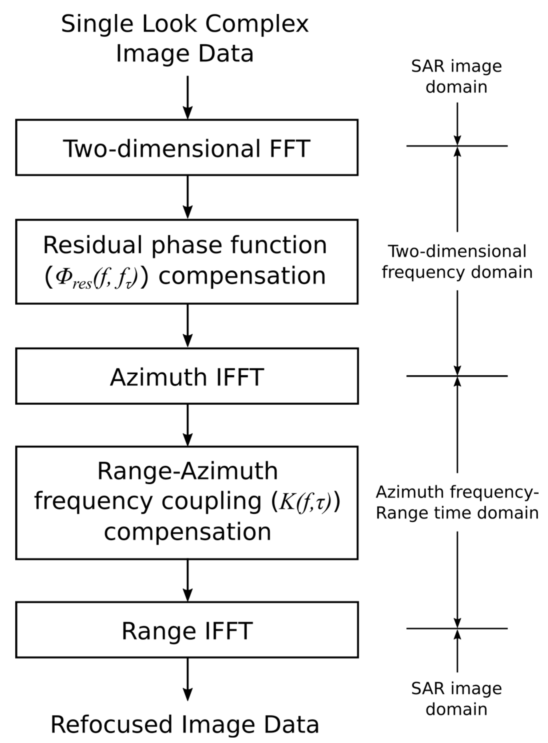
In summary, there is a wide variety of approaches for Doppler parameter estimation. Since the efficiency of each method largely depends on the system parameters and configuration, one should carefully examine the properties of a given system and data. Once the Doppler parameters and velocity are retrieved from a given SAR SLC data, the next step is to apply the residual focusing. As described in the previous section, the proposed algorithm consists of two phase-multiplications in two different domains. Figure 3 shows the entire operations in the proposed correction scheme. Note that the residual phase, , and the range-azimuth frequency coupling, , in Figure 3 correspond to the Equations (11) and (17), respectively. Since the data has already been azimuth and range compressed, and the signal bandwidth of the moving target remains unchanged after taking a subset in the time domain, it would be sufficient to use a limited window size for the processing. From various tests, a sub-window of 64 × 64 is large enough for high-resolution, X-band SLC data from space-borne SAR such as TerraSAR-X and COSMO-SkyMed.
4. Simulation and Application Results
4.1. Simulation Results
Simulation tests have been carried out as follows using the system parameters of the TerraSAR-X stripmap mode (Table 1). First, SAR raw signals were simulated with a point target which moved at 45° oblique to the azimuth and range directions with various velocities ranging from −30 m/s to +30 m/s with 1 m/s interval. The motion of the point target was assumed to be constant, i.e., without acceleration for simplicity, as the effect of acceleration is often insignificant in the case of the space-born SAR stripmap mode, which has a relatively short azimuth integration time (for instance, less than 0.6 s for TerraSAR-X). The simulated raw signals were then focused into standard SLC images using a chirp-scaling algorithm [32]. After detection and Doppler parameter estimation of each moving target, a sub window of 64 × 64 centered on the moving target was extracted and then corrected by applying the proposed method. To evaluate the performance of the method, we substituted the exact motion parameters into the fine-tuning filter, which means that there was no error in the detection and Doppler parameter estimation scheme. Finally, various quality parameters were measured from both the original and fine-tuned SLC images in order to evaluate the improvement achieved by the proposed refocusing method. Three parameters are typically used for SAR point target quality assessment: −3 dB width, integrated sidelobe ratio (ISLR), and symmetry. The −3 dB width is commonly used for spatial resolution estimation. Since the reconstructed signal from a moving point target is asymmetrical and the side lobe is difficult to determine, ISLR is used instead of the peak sidelobe ratio (PSLR). Figure 4a,b show −3 dB widths of both directions with varying moving speeds for the point target. Before applying the fine-tuning, the spatial resolution in the azimuth direction degrades rapidly as the target speed increases, while that in the range direction shows no significant changes. After applying the fine-tuning process, the spatial resolution in the azimuth direction is significantly improved. There is a small amount of residual broadening in the azimuth direction, which is proportional to the target speed. The ISLR in Figure 4c,d display the ISLR in both the azimuth and range directions. The azimuth ISLR increases steeply as the target speed increases up to −3 dB, while the range ISLR is almost unaffected by the target’s motion. The improvement in the azimuth direction is significant particularly up to about 8 m/s (or 28.8 km/h).
Symmetry is a measure of the energy balance of the compressed signal. In order to measure this quantity, we decomposed the power of the compressed signal into symmetric and antisymmetric parts as follows:
where is a cell number along range or azimuth, axis centered at 0, which ranges between and where is the size of fine-tuning filter. Note that and are essentially symmetric and anti-symmetric, respectively. Then, the symmetry can be measured from vector norms () as follows:
which ranges from 0 (fully anti-symmetric) to 1 (fully symmetric). Figure 5 displays the changes of symmetry in both azimuth and range. As expected, the symmetry also becomes worse as the target’s speed increases. Unlike the former two measures, the symmetry relies on range velocity. The simulation with varying speed only in the azimuth component showed no changes in symmetry. This is based on the fact that the range migration of a scatterer moving in the range direction is asymmetrical to the closest range distance, while that of a scatterer moving in the azimuth direction is fully symmetric in a zero-Doppler geometry. It may be of interest to note that all three parameters change abruptly when the target moves at around 8 m/s. This is nearly coincident with the moment when the peak power of a focused range cell migrates into the next range cell. This range walk effect is abrupt and discrete. Since we set the range center of the fine-tuning window to where we observe the maximum energy of the blurred target in units of integer number, the change in range cell number leads to inaccurate selection of the range distance, which is required for generating a proper filter. Consequently, the apparent performance of the algorithm, based on the quality parameters, seems to be gradually reduced; however, the overall achievement by the fine-tuning filter is sufficiently high to retrieve the target’s true nature. The maximum error of post-correction in our simulation in the 30 m/s case was comparable to that of pre-correction at 3 m/s or less.
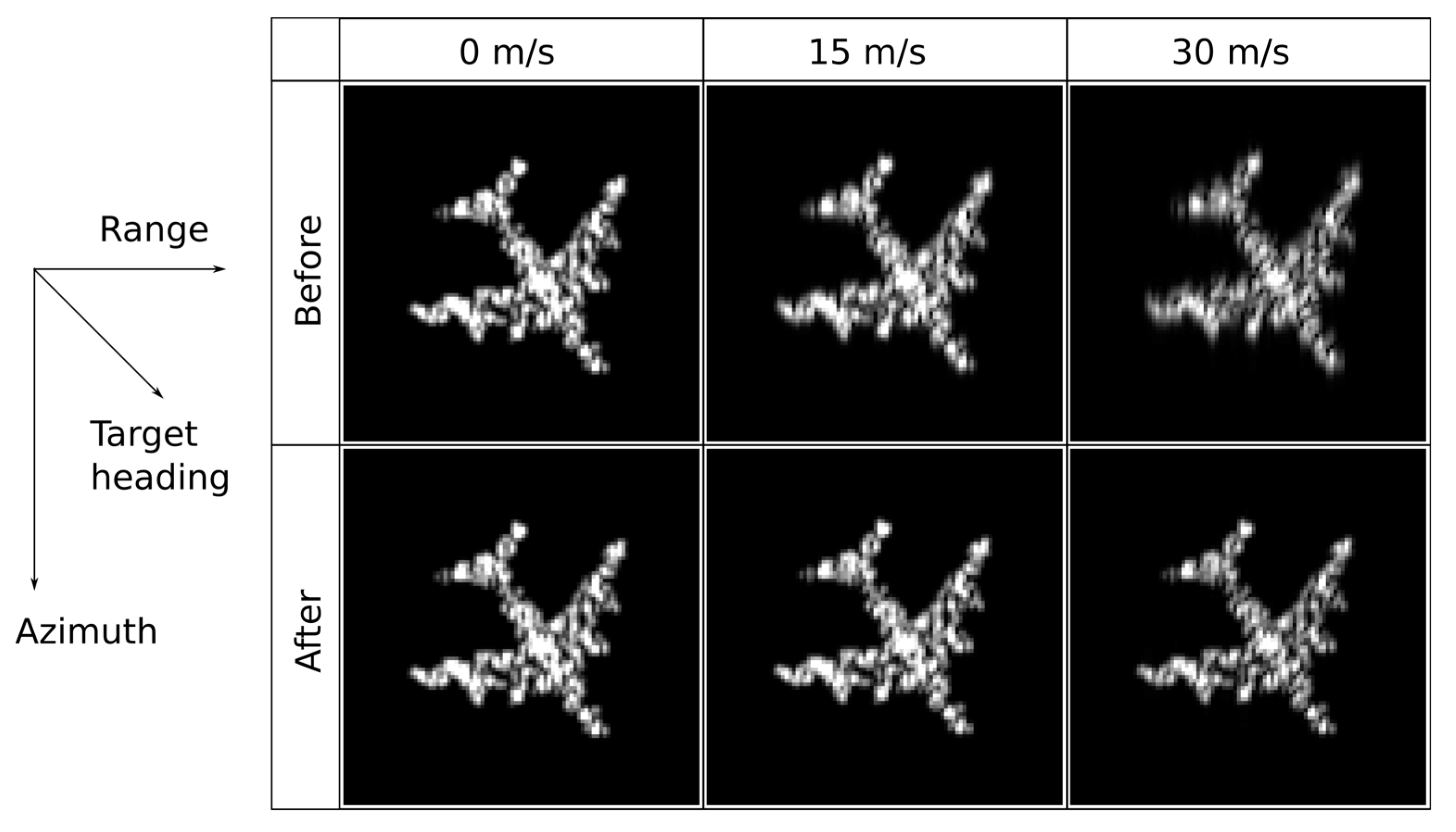
Although the quantitative performance evaluation was carried out using a point target simulation, a visual interpretation of the correction result for an extended target helps to convey how the image is restored. Figure 6 shows a simulated aircraft taxiing on the ground. The upper panels show the normally focused images, and the lower panels show the corresponding fine-tuned images. The correction results are not only well focused but also shifted a bit in the range direction because of the correction for the range walk.
4.2. Example of Application to TerraSAR-X Data
Test data were obtained by TerraSAR-X from a speed-controlled vehicle moving on the road with velocities of −6.6 and −13.8 m/s (or −23.8 and −49.6 km/h, respectively) in the azimuth and range directions, respectively. The speed of the vehicle was precisely measured by GPS as well as speedometer, and was retrieved from the TerrSAR-X data itself by Doppler frequency analysis. The details of the data used in the test and velocity retrieval process are given in [45]. The application result is shown in Figure 7 and Figure 8, which demonstrate the effectiveness of the proposed fine-tuning tactics for high-resolution SAR SLC data.
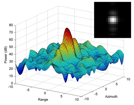
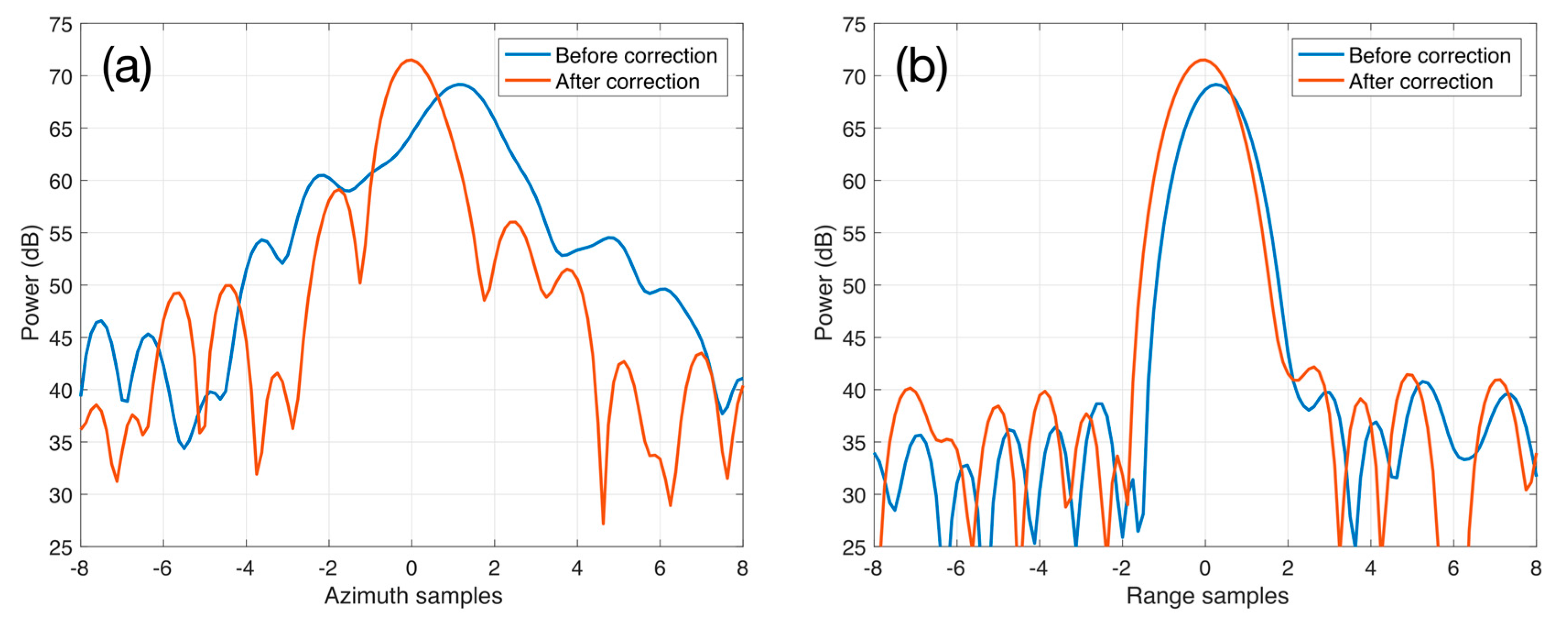
As seen in Figure 7 and Figure 8, the target movement caused significant energy dispersion (or image blurring) in the azimuth and range directions, losing the symmetry of the typical sinc function, and causing a slight shift of peak locations along both the azimuth and range. Image blurring in the azimuth (see Figure 7a and Figure 9a) has been previously well known, and the improvement of the peak sidelobe ratio is about 4 dB in this example. In addition to image blurring, asymmetry of the compressed signal in the azimuth direction is significant, as in Figure 8a. The symmetry value of 0.92 in the azimuth of the original SLC data is improved to 0.94 after fine-tuning. Also, this resulted in distortion removal of the target shape. Slight shifts in the peak locations by about 1.1 samples (or 2.13 m) and 0.3 samples (or 0.65 m) in the azimuth and ground range directions are also noted. The residual range compression by Equation (14) is, however, not significant in this example because the value of is relatively small compared with those of and .
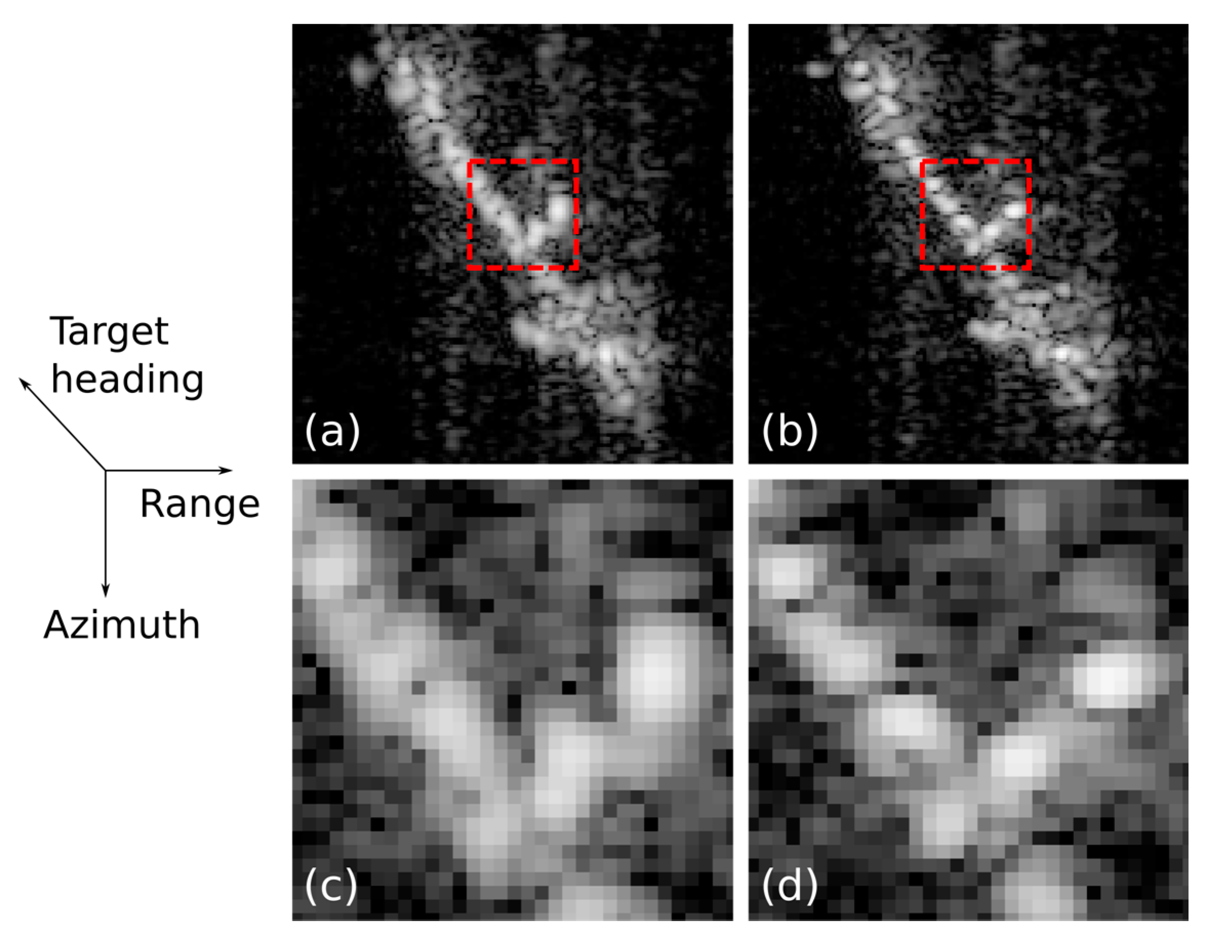
Besides the speed-controlled target, there were several other moving objects in the same test image. As an example of the extended target, Figure 9 shows a large ship moving along an oblique to the azimuth and range direction. Although an in-situ measurement for the movement was not available, the joint time-frequency analysis [45] was used for the velocity estimation. The estimated velocity was −5.6 and −5.1 m/s (or −20.1 and 18.4 km/h) in the azimuth and range directions, respectively. Although the simulation results showed in the previous section indicates that the distortion would not be serious compared to the case with velocities higher than 8 m/s, the original image and the corresponding fine-tuned image in Figure 9a,b have notable differences.
Unlike the small object in Figure 7, this target is extended to few tens of pixels, and the radar reflectivities along the ship orientation look not much changing in the scaled image in Figure 9c. However, the fine-tuned image in Figure 9d indicates that the ship body actually has a structure with countable prominent points.
5. Discussion
Both simulation and TerraSAR-X results demonstrated the capability of the proposed method to improve the signal compression of ground moving objects. The improvement is a function of the target speed and monotonically is increased with the target speed up to 20 m/s. When the target speed was 7 m/s, the simulated signal in the azimuth direction was improved by 134% and 196% in −3 dB width and ISLR, respectively. The application to the TerraSAR-X also showed similar results with an improvement of 193% in −3 dB width for the vehicle whose speed was controlled at an azimuth velocity of 6.6 m/s. It should also be noted that the improvement of the compression ratio and peak sidelobe ratio was by about 4 dB. The refocused object was also shifted to the true position by about 1.1 and 0.3 samples in the azimuth and range direction, respectively. Symmetry of the compressed signal is also important to characterize the target, and the proposed method improved the symmetry by up to 0.94. Various SAR focusing methods have derived from raw radar signals [9,12], but they are neither computationally efficient nor practically applicable because of the data distribution policy of most high resolution SAR data. Among recent publications, the methods in [46,47] deal with a similar topic of ground moving target imaging. The method in [46] adopted the Stolt interpolation in the 2D frequency domain. Although the compression ratio of the method was very competitive, the asymmetric sidelobes were not fully suppressed [47]. A symmetry of 0.94 achieved from the TerraSAR-X results of this study in Figure 8 showed the superior performance of the proposed method. An improved method was also proposed by [47], which exploits the parameter sparse representation method and iteration. Image entropy and symmetry of compressed signals were significantly improved by the method in [47]. As far as the performance of refocusing is concerned, the method in [47] is superior to [46] at the cost of computational efficiency. The method in [47] reached the state of convergence after about one hundred iterations which significantly increased computation time.
As discussed before, the main advantages of the proposed method are twofold. First, the proposed residual focusing is based on the derived formulae of the Doppler spectrum after conventional image formation. Second, the method is simple and practically applicable to SLC data of high-resolution SAR systems. Although the proposed method demonstrated the competitive ability of residual focusing, it does have some limitations. First, the correction formulae in Equations (12)–(14) are approximated to the second-order terms, and consequently the effects of high-order terms remain to be further accounted. Second, the final quality of the residual focused SAR image depends on the accuracy of the Doppler parameters used for processing. The Doppler parameters can be obtained by parameter estimation from SLC data, which is beyond the scope of this paper. A number of approaches for Doppler parameter estimation have been developed and typical examples are referred to in [43,44,45]. One should carefully examine the properties of a given system and data before Doppler parameter estimation because the efficiency of each method largely depends on the system parameters and configuration. Third, the coupling of the azimuth and range frequencies in the SLC data described in Equation (16) and Figure 2 is sensitive to the slope which is a function of the range velocity of the target, the incidence angle, and the wavelength. A more sophisticated approach than the simple phase compensation by Equation (17) might be necessary if a further refinement in range dimension is required. For this purpose, raw SAR signals rather than SLC data should be involved in the processing.
6. Conclusions
Theoretical formulae were derived for the fine-tuning of ground moving targets in SAR SLC data and processing tactics were proposed. The proposed fine-tuning significantly improved the image quality in three aspects: residual compression, the symmetry of the compressed signal in both the azimuth and range directions, and the slight shift of the peak positions. While various focusing methods for SAR raw signals have been developed previously, a general approach for SAR SLC data has not been well investigated. The proposed method is practical for post-processing of SAR SLC data by general users. The importance of the method lies in the fact that most SAR data provided to general users are SLC data rather than raw signals. The residual focusing is simple and straightforward, based on an elaborately derived residual Doppler spectrum with a relatively small processing window. Simulation results support that the target’s motion deteriorates image quality particularly in azimuth in terms of the −3 dB width, ISLR, and asymmetry, and the proposed fine-tuning efficiently restores the image quality. It may be of interest to note that all three parameters (−3 dB width, ISLR and asymmetry) change abruptly when the target moves faster than 8 m/s. The application results using TerraSAR-X and a speed-controlled ground moving vehicle demonstrate the effectiveness of the method without a heavy computational burden. The residual focusing ideally reconstructs ground moving targets with particular improvements of the compression ratio and symmetry.
Acknowledgments
This work was supported by the National Space Lab program through the Korea Science and Engineering Foundation funded by the Ministry of Science, ICT and Future Planning (2013M1A3A3A02042314. The TerraSAR-X data were provided to J.-S. Won as a part of TerraSAR-X Science Team Project (PI No. COA0047).
Author Contributions
J.-S. Won conceived the main idea; J.-W. Park and J.H. Kim performed the experiments; J.-W. Park and J.-S. Won analyzed the data and wrote the paper.
Conflicts of Interest
The authors declare no conflict of interest.
References
- Raney, R.K. Synthetic aperture imaging radar and moving targets. IEEE Trans. Aerosp. Electron. Syst. 1971, 7, 499–505. [Google Scholar] [CrossRef]
- Werness, S.; Carrara, W.; Joyce, L.; Franczak, D. Moving target imaging algorithm for SAR data. IEEE Trans. Aerosp. Electron. Syst. 1990, 26, 57–67. [Google Scholar] [CrossRef]
- Kirscht, M. Detection and imaging or arbitrarily moving targets with single-channel SAR. In Proceedings of the 2002 International Radar Conference, Edinburgh, UK, 15–17 October 2002. [Google Scholar] [CrossRef]
- Linnehan, R.; Perlovsky, L.; Mutz, I.C.; Rangaswamy, M.; Schindler, J. Detecting multiple slow-moving targets in SAR images. In Proceedings of the Sensor Array and Multichannel Signal Processing Workshop, Barcelona, Spain, 18–21 July 2004; pp. 643–647. [Google Scholar]
- Marques, P.A.C.; Dias, J.M.B. Velocity estimation of fast moving targets using a single SAR sensor. IEEE Trans. Aerosp. Electron. Syst. 2005, 41, 75–89. [Google Scholar] [CrossRef]
- Weihing, D.; Hinz, S.; Meyer, F.; Laika, A.; Bamler, R. Detection of along-track ground moving targets in high resolution spaceborn SAR images. In Proceedings of the ISPRS Commission VII Symposium, Enschede, The Netherlands, 8–11 May 2006; pp. 81–85. [Google Scholar]
- Meyer, F.; Hinz, S.; Laika, A.; Suchandt, S.; Bamler, R. Performance analysis of space-borne SAR vehicle detection and velocity estimation. In Proceedings of the ISPRS Commission III Symposium, Born, Germany, 20–22 September 2006. [Google Scholar]
- Baumgartner, S.V.; Krieger, G. Fast GMTI algorithm for traffic monitoring based on a priori knowledge. IEEE Trans. Geosci. Remote Sens. 2012, 50, 4626–4641. [Google Scholar] [CrossRef] [Green Version]
- Chen, C.C.; Andrews, H.C. Target motion induced radar imaging. IEEE Trans. Aerosp. Electron. Syst. 1980, 16, 2–14. [Google Scholar] [CrossRef]
- Freeman, A.; Currie, A. Synthetic aperture radar (SAR) images of moving targets. GEC J. Res. 1987, 5, 106–115. [Google Scholar]
- Moreira, J.R.; Keydel, W. A new MTI-SAR approach using the reflectivity displacement method. IEEE Trans. Geosci. Remote Sens. 1995, 33, 1238–1244. [Google Scholar] [CrossRef]
- Fienup, J.P. Detecting moving targets in SAR imagery by focusing. IEEE Trans. Aerosp. Electron. Syst. 2001, 37, 749–809. [Google Scholar]
- Pettersson, M. Extraction of moving ground targets by a bistatic ultra-wideband SAR. IEE Proc. Radar Sonar Navig. 2001, 148, 35–49. [Google Scholar] [CrossRef]
- Dias, J.M.B.; Marques, P.A.C. Multiple moving target detection and trajectory estimation using a single SAR sensor. IEEE Trans. Aerosp. Electron. Syst. 2003, 39, 604–624. [Google Scholar] [CrossRef]
- Sparr, T. Moving target motion estimation and focusing in SAR images. In Proceedings of the IEEE Radar Conference, Arlington, VA, USA, 9–12 May 2005; pp. 290–294. [Google Scholar]
- Chapman, R.D.; Hawes, C.M.; Nord, M.E. Target motion ambiguities in single-aperture synthetic aperture radar. IEEE Trans. Aerosp. Electron. Syst. 2010, 46, 459–468. [Google Scholar] [CrossRef]
- Goldstein, R.; Zebker, H. Interferometric radar measurements of ocean surface currents. Nature 1987, 328, 707–709. [Google Scholar] [CrossRef]
- Rodriguez, E.; Martin, J.M. Theory and design of interferometric synthetic aperture radars. IEE Proc. F Radar Signal Process. 1992, 139, 147–159. [Google Scholar] [CrossRef]
- Ainsworth, T.; Chubb, S.; Fusina, R.; Goldstein, R.; Jansen, R.; Lee, J.; Valenzuela, G. InSAR imagery of surface currents, wave fields, and fronts. IEEE Trans. Geosci. Remote Sens. 1995, 33, 1117–1123. [Google Scholar] [CrossRef]
- Soumekh, M. Moving target detection in foliage using along track monopulse synthetic aperture radar imaging. IEEE Trans. Image Process. 1997, 6, 1148–1163. [Google Scholar] [CrossRef] [PubMed]
- Romeiser, R.; Thompson, D.R. Numerical study on the along-track interferometric radar imaging mechanism of oceanic surface currents. IEEE Trans. Geosci. Remote Sens. 2000, 38, 446–458. [Google Scholar] [CrossRef]
- Rosen, P.; Hensley, S.; Joughin, I.; Li, F.; Madsen, S.; Rodriguez, E.; Goldstein, R. Synthetic aperture radar interferometry. Proc. IEEE 2000, 88, 333–382. [Google Scholar] [CrossRef]
- Moccia, A.; Rufino, G. Spaceborne along-track SAR interferometry: performance analysis and mission scenarios. IEEE Trans. Aerosp. Electron. Syst. 2001, 37, 199–213. [Google Scholar] [CrossRef]
- Chen, C.W. Performance assessment of along-track interferometry for detecting ground moving targets. In Proceedings of the IEEE Radar Conference, Philadelphia, PA, USA, 26–29 April 2004; pp. 99–104. [Google Scholar]
- Chiu, S.; Livingstone, C.E. A comparison of displaced phase centre antenna and along-track interferometry techniques for RADARSAT-2 ground moving target indication. Can. J. Remote Sens. 2005, 31, 37–51. [Google Scholar] [CrossRef]
- Gierull, C.H.; Cerutti-Maori, D.; Ender, J.H.G. Ground moving target indication with tandem satellite constellations. IEEE Geosci. Remote Sens. Lett. 2008, 5, 710–714. [Google Scholar] [CrossRef]
- Yang, L.; Wang, T.; Bao, Z. Ground moving target indication using an InSAR system with a hybrid baseline. IEEE Geosci. Remote Sens. Lett. 2008, 5, 373–377. [Google Scholar] [CrossRef]
- Cerutti-Maori, D.; Gierull, C.H.; Ender, J.H.G. Experimental verification of SAR-GMTI improvement through antenna switching. IEEE Trans. Geosci. Remote Sens. 2010, 48, 2066–2075. [Google Scholar] [CrossRef]
- Kirkland, D. Imaging moving targets using the second-order keystone transform. IET Radar Sonar Navig. 2011, 5, 902–910. [Google Scholar] [CrossRef]
- Sun, G.; Xing, M.; Xia, X.-G.; Wu, Y.; Bao, Z. Robust ground moving-target imaging using deramp-keystone processing. IEEE Trans. Geosci. Remote Sens. 2013, 51, 966–982. [Google Scholar] [CrossRef]
- Yang, J.; Liu, C.; Wang, Y. Imaging and parameter estimation of fast-moving targets with single-antenna SAR. IEEE Geosci. Remote Sens. Lett. 2014, 11, 529–533. [Google Scholar] [CrossRef]
- Raney, R.K.; Runge, H.; Bamler, R.; Cumming, I.G.; Wong, F.H. Precision SAR processing using chirp scaling. IEEE Trans. Geosci. Remote Sens. 1994, 32, 786–799. [Google Scholar] [CrossRef]
- Bamler, R. A comparison of range-Doppler and wavenumber domain SAR focusing algorithms. IEEE Trans. Geosci. Remote Sens. 1992, 30, 706–713. [Google Scholar] [CrossRef]
- Moreira, A.; Mittermayer, J.; Scheiber, R. Extended chirp scaling algorithm for air- and spaceborne SAR data processing in stripmap and ScanSAR imaging modes. IEEE Trans. Geosci. Remote Sens. 1996, 34, 1123–1136. [Google Scholar] [CrossRef]
- Perry, P.R.; DiPietro, R.C.; Fante, R. SAR imaging of moving targets. IEEE Trans. Aerosp. Electron. Syst. 1999, 35, 188–200. [Google Scholar] [CrossRef]
- Zhou, F.; Wu, R.; Xing, M.; Bao, Z. Approach for single channel SAR ground moving target imaging and motion parameter estimation. IET Radar Sonar Navig. 2007, 1, 59–66. [Google Scholar] [CrossRef]
- Kirkland, D. Using the keystone transform for detection of moving targets. In Proceedings of the EUSAR, Aachen, Germany, 7–10 June 2010; pp. 305–308. [Google Scholar]
- Kirkland, D.M. An alternative range migration correction algorithm for focusing moving targets. Prog. Electromagn. Res. 2012, 131, 227–241. [Google Scholar] [CrossRef]
- Raney, R.K. Considerations for SAR image quantification unique to orbital systems. IEEE Trans. Geosci. Remote Sens. 1991, 29, 754–760. [Google Scholar] [CrossRef]
- Barbarossa, S.; Farina, A. Space-time-frequency processing of synthetic aperture radar signals. IEEE Trans. Aerosp. Electron. Syst. 1994, 30, 341–358. [Google Scholar] [CrossRef]
- Barbarossa, S. Detection and imaging of moving objects with synthetic aperture radar. Part 1. Optimal detection and parameter estimation theory. IEE Proc. F Radar Signal Process. 1992, 139, 79–88. [Google Scholar] [CrossRef]
- Barbarossa, S.; Farina, A. Detection and imaging of moving objects with synthetic aperture radar. Part 2: Joint time-frequency analysis by Wigner-Ville distribution. IEE Proc. F Radar Signal Process. 1992, 139, 89–97. [Google Scholar] [CrossRef]
- Kersten, P.R.; Janse, R.W.; Luc, K.; Ainsworth, T.L. Motion analysis in SAR images of unfocused objects using time-frequency methods. IEEE Trans. Geosci. Remote Sens. Lett. 2007, 4, 527–531. [Google Scholar] [CrossRef]
- Kersten, P.R.; Topokov, J.V.; Ainsworth, T.L.; Sletten, M.A.; Jansen, R.W. Estimating surface water speeds with a single-phase center SAR versus an along-track interferometric SAR. IEEE Trans. Geosci. Remote Sens. 2010, 48, 3638–3646. [Google Scholar] [CrossRef]
- Park, J.-W.; Won, J.-S. An efficient method of Doppler parameter estimation in the time-frequency domain for a moving object from TerraSAR-X data. IEEE Trans. Geosci. Remote Sens. 2011, 49, 4771–4787. [Google Scholar] [CrossRef]
- Zhang, Y.; Sun, J.; Lei, P.; Li, G.; Hong, W. High-resolution SAR-based ground moving target imaging with defocused ROI data. IEEE Trans. Geosci. Remote Sens. 2016, 54, 1062–1073. [Google Scholar] [CrossRef]
- Chen, Y.; Li, G.; Zhang, Q.; Sun, J. Refocusing of Moving Targets in SAR Images via Parametric Sparse Representation. Remote Sens. 2017, 9, 795. [Google Scholar] [CrossRef]
- Livingstone, C.; Sikaneta, I.; Gierull, C.H.; Chiu, S.; Beaudoin, A.; Campbell, J.; Beaudoin, J.; Gong, S.; Knight, T. An airborne SAR experiment to support RADARSAT-2 GMTI. Can. J. Remote Sens. 2002, 28, 1–20. [Google Scholar] [CrossRef]
- Gierull, C.H. Ground moving target parameter estimation for two-channel SAR. IEE Proc. Radar Sonar Navig. 2006, 153, 224–233. [Google Scholar] [CrossRef]
- Cerutti-Maori, D.; Sikaneta, I. Generalization of DPCA processing for multichannel SAR/GMTI radars. IEEE Trans. Geosci. Remote Sens. 2013, 51, 560–572. [Google Scholar] [CrossRef]
- Suchandt, S.; Runge, H.; Breit, H.; Steinbrecher, U.; Kotenkov, A.; Balss, U. Automatic extraction of traffic flows using TerraSAR-X along-track interferometry. IEEE Trans. Geosci. Remote Sens. 2010, 48, 807–819. [Google Scholar] [CrossRef]
- Ender, J.H.G. Space-time processing for multichannel synthetic aperture radar. Electron. Commun. Eng. J. 1999, 11, 29–38. [Google Scholar] [CrossRef]
- Melvin, W.L. A STAP overview. IEEE Aerosp. Electron. Syst. Mag. 2004, 19, 19–35. [Google Scholar] [CrossRef]
- Sharma, J.; Gierull, C.H.; Collins, M.J. The influence of target acceleration on velocity estimation in dual-channel SAR-GMTI. IEEE Trans. Geosci. Remote Sens. 2006, 44, 134–147. [Google Scholar] [CrossRef]
Figure 1.
A stripmap synthetic aperture radar (SAR) observation geometry for a ground moving object.
Figure 1.
A stripmap synthetic aperture radar (SAR) observation geometry for a ground moving object.
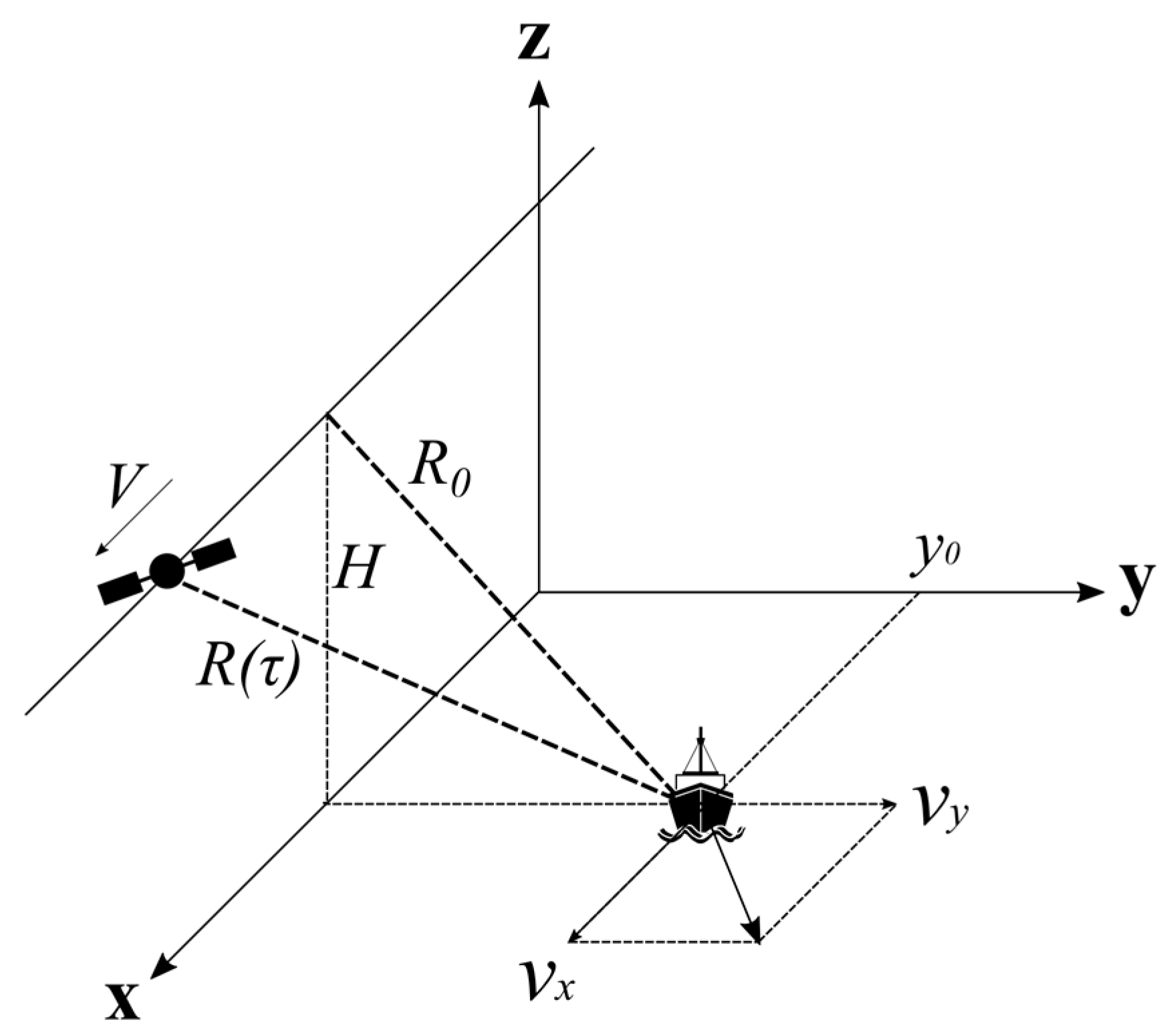
Figure 2.
Schematic of the effect of residual phase in the range frequency-azimuth time domain. The coupling between the range and azimuth frequencies projects the azimuth-compressed signals on a slanted line rather than a horizontal line in the range frequency-azimuth time domain. The slope largely depends on (or ); consequently, the ground object with large range speed suffers a significant distortion.

Figure 3.
The operations in the proposed correction algorithm, which consists of two phase-multiplications in two different domains.
Figure 3.
The operations in the proposed correction algorithm, which consists of two phase-multiplications in two different domains.

Figure 4.
Simulation results of the −3 dB width and the integrated sidelobe ratio (ISLR) in the (a,c) azimuth and (b,d) range directions, respectively. The simulation was carried out using system parameters of the TerraSAR-X stripmap mode (see Table 1). The improvement in the azimuth direction is significant particularly up to about 8 m/s (or 28.8 km/h).
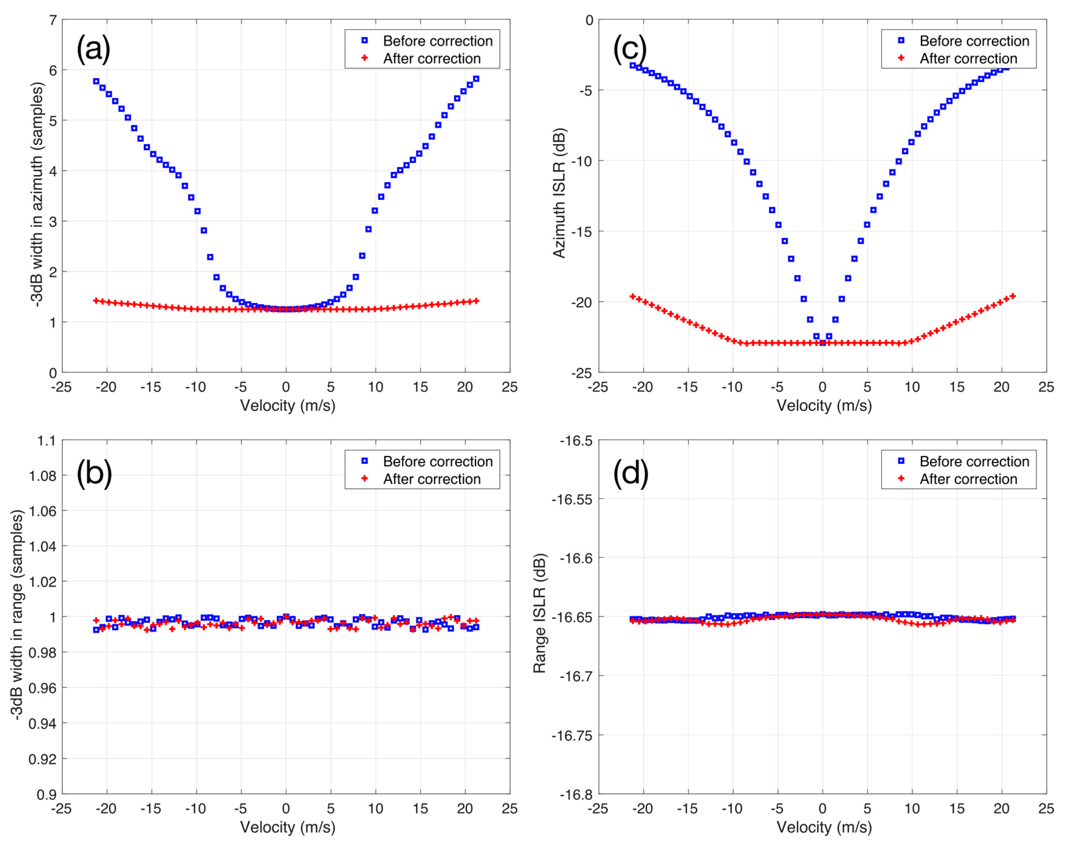
Figure 5.
Simulation results of (a) azimuth and (b) range symmetry of the reconstructed signals. While the range symmetry was not seriously affected by the target’s moving speed, the azimuthal symmetry deteriorated when the moving speed was higher than 8 m/s. The azimuthal symmetry is well recovered by the proposed method as in (a).
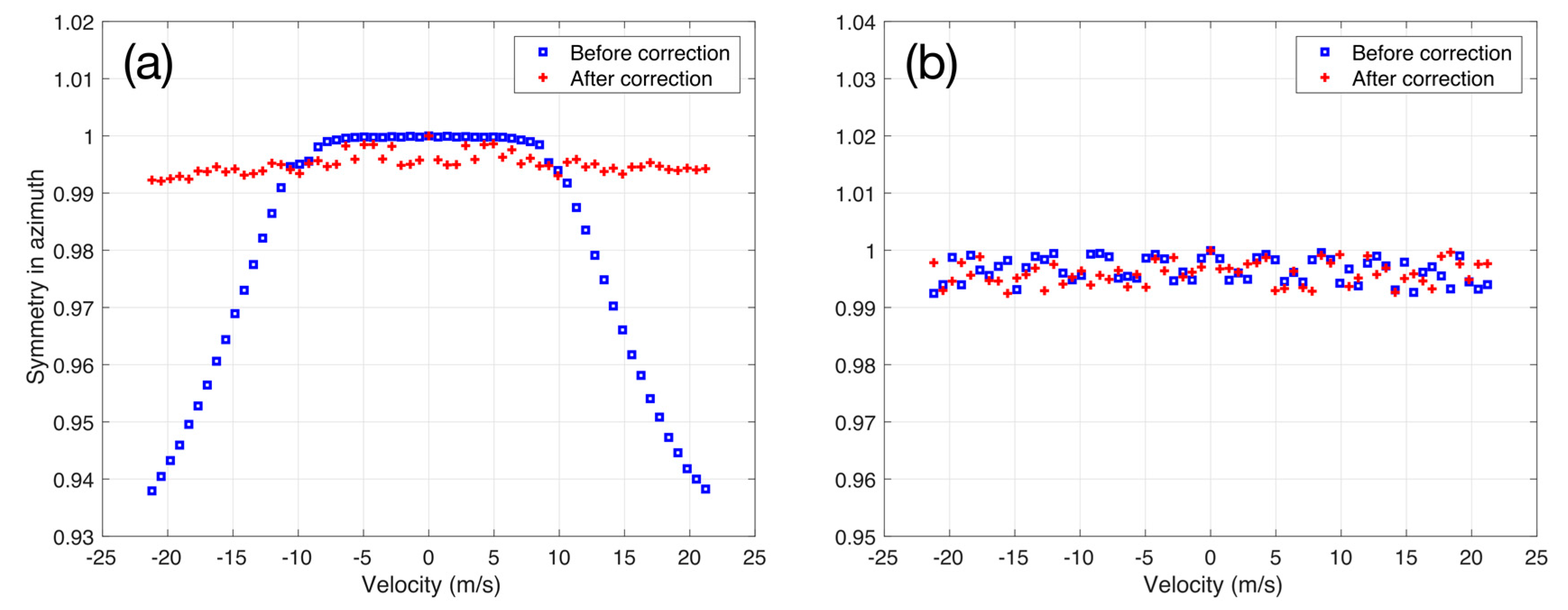
Figure 6.
Simulation results of an extended target with varying velocities. The upper panels are for the single-look complex (SLC) sub-images processed by a standard synthetic aperture radar (SAR) focusing, and the lower panels for the fine-tuned images processed by the proposed algorithm. The fine-tuned images are not only well focused but also shifted a bit in the range direction because of the correction for the range walk.

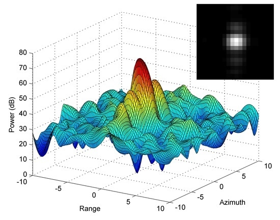
Figure 7.
Sub-window image and power distribution of (a) the original SLC data and (b) the data after removing the residual phase. (c) The test was carried out using a speed-controlled vehicle moved with velocities of −6.6 and −13.8 m/s (or −23.8 and −49.6 km/h, respectively) in the azimuth and range directions, respectively [45]. Note the improvement of symmetry around the target as well as improvement of the compression ratio and peak sidelobe ratio by about 4 dB.
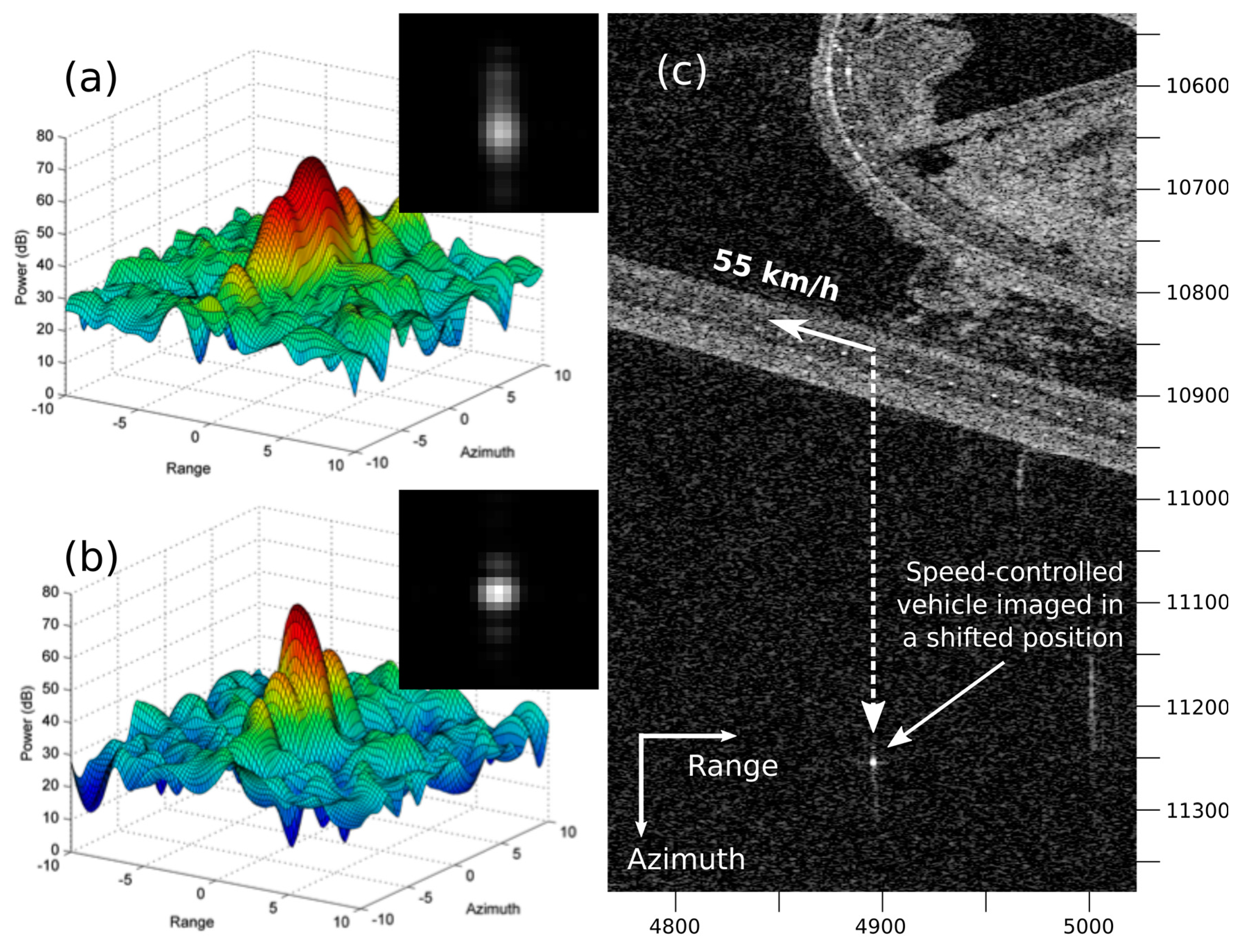
Figure 8.
Power profiles crossing the center of the ground moving vehicle along the (a) azimuth and (b) range directions in Figure 7. Note the improvement in the peak sidelobe ratio by about 4 dB and that in the symmetry from 0.92 to 0.94 in the azimuth dimension, as in (a). In addition, the refocused object shifted by about 1.1 and 0.3 samples in azimuth and range direction, respectively.

Figure 9.
A moving ship observed in (a) the original SLC data and (b) the data after removing the residual phase. The original image size here is 64 by 64 pixels, however, the image was interpolated by a factor of two in order to show the details. The estimated velocity by using the joint time-frequency analysis [45] was −5.6 and −5.1 m/s (or −20.1 and −18.4 km/h, respectively) in the azimuth and range directions, respectively. Although the target speed is low considering the image distortion rapidly increases with speed higher than 8 m/s as noted in the simulation test, the scaled images, (c,d) show clear improvement in image focusing.

Table 1.
Summary of sensor model parameters used for simulation
| Parameter | Value |
|---|---|
| Chirp length | 47.17 μm |
| Range sampling rate | 109.88 MHz |
| Chirp bandwidth | 100 MHz |
| Carrier frequency | 9.65 GHz |
| Antenna length | 4.8 m |
| Effective velocity | 7371.1 m/s |
| Pulse repetition frequency | 3815.49 Hz |
| Slant range to scene center | 650.79 km |
| Indicence angle at scene center | 39.24° |
| Doppler centroid | 0 Hz |
| Sensor height | 513.08 km |
© 2017 by the authors. Licensee MDPI, Basel, Switzerland. This article is an open access article distributed under the terms and conditions of the Creative Commons Attribution (CC BY) license (http://creativecommons.org/licenses/by/4.0/).
Share and Cite
MDPI and ACS Style
Park, J.-W.; Kim, J.H.; Won, J.-S. Fast and Efficient Correction of Ground Moving Targets in a Synthetic Aperture Radar, Single-Look Complex Image. Remote Sens. 2017, 9, 926. https://doi.org/10.3390/rs9090926
AMA Style
Park J-W, Kim JH, Won J-S. Fast and Efficient Correction of Ground Moving Targets in a Synthetic Aperture Radar, Single-Look Complex Image. Remote Sensing. 2017; 9(9):926. https://doi.org/10.3390/rs9090926
Chicago/Turabian StylePark, Jeong-Won, Jae Hun Kim, and Joong-Sun Won. 2017. "Fast and Efficient Correction of Ground Moving Targets in a Synthetic Aperture Radar, Single-Look Complex Image" Remote Sensing 9, no. 9: 926. https://doi.org/10.3390/rs9090926
Note that from the first issue of 2016, this journal uses article numbers instead of page numbers. See further details here.