Detecting Drought-Induced Tree Mortality in Sierra Nevada Forests with Time Series of Satellite Data

Department of Land, Air and Water Resources, University of California, Davis, CA 95616-8627, USA
*
Author to whom correspondence should be addressed.
Remote Sens. 2017, 9(9), 929; https://doi.org/10.3390/rs9090929
Submission received: 22 July 2017
/
Revised: 15 August 2017
/
Accepted: 31 August 2017
/
Published: 8 September 2017
(This article belongs to the Section Forest Remote Sensing)
Abstract
:A five-year drought in California led to a significant increase in tree mortality in the Sierra Nevada forests from 2012 to 2016. Landscape level monitoring of forest health and tree dieback is critical for vegetation and disaster management strategies. We examined the capability of multispectral imagery from the Moderate Resolution Imaging Spectroradiometer (MODIS) in detecting and explaining the impacts of the recent severe drought in Sierra Nevada forests. Remote sensing metrics were developed to represent baseline forest health conditions and drought stress using time series of MODIS vegetation indices (VIs) and a water index. We used Random Forest algorithms, trained with forest aerial detection surveys data, to detect tree mortality based on the remote sensing metrics and topographical variables. Map estimates of tree mortality demonstrated that our two-stage Random Forest models were capable of detecting the spatial patterns and severity of tree mortality, with an overall producer’s accuracy of 96.3% for the classification Random Forest (CRF) and a RMSE of 7.19 dead trees per acre for the regression Random Forest (RRF). The overall omission errors of the CRF ranged from 19% for the severe mortality class to 27% for the low mortality class. Interpretations of the models revealed that forests with higher productivity preceding the onset of drought were more vulnerable to drought stress and, consequently, more likely to experience tree mortality. This method highlights the importance of incorporating baseline forest health data and measurements of drought stress in understanding forest response to severe drought.
1. Introduction
Sierra Nevada (SN) forests provide critical environmental, social, and economic services throughout California [1,2,3,4]. However, a warmer and drier climate and decades of active land management have changed forest compositions and functions notably, affecting forest resilience to extreme climatic events and potentially their long term sustainability [1,5,6,7,8]. This region experienced five consecutive years of severe drought starting in 2012, due to persistent lower-than-normal precipitation and hotter temperatures. A state emergency of drought was declared in 2014 until the record-breaking precipitation events of 2017 [1,7,9]. The prolonged drought has resulted in more than 100 million dead trees in California since 2010, with more than 35 million trees having died in the summer of 2016 [4]. The growing extent of dead and dying trees poses immediate threats to public safety and creates flammable fuel for potential large and intense wildfires. Cascading effects of this massive die-off are profound and long lasting, including changes in water availability and quality, fire regimes, forest composition, species shifts, and feedback to atmospheric and climatic processes [3,8,10,11,12,13].
Typical drivers of regional tree mortality include extreme climate variability, wildfire, insect outbreaks, and carbon starvation following hydraulic failure [5,8,14,15,16,17]. Drought conditions exacerbate the impacts of these disturbances, increasing the extent and severity of forest mortality events [3,18,19]. The underlying mechanisms of drought-induced tree mortality can be direct or indirect. Hydraulic failure from moisture deficits limits the photosynthetic capacity of trees and impedes growth, weakening trees and disrupting their normal phenology [20]. Weakened trees can succumb to mortality through carbon starvation or greater exposure to drought-related disturbances including biotic attacks from insects and pathogens [3,15,21]. Less severe winter temperatures allow the populations of insects, such as bark beetles, to flourish [6,22]. Denser forests from a history of fire suppression ease the dispersal of these populations, increasing rates of defoliation, desiccation, browning, and mortality [3,23,24,25]. In a changing climate, it is expected that regional precipitation will become more variable and temperatures will rise, leading to more frequent and long-lasting “hotter droughts” [6,10,26]. Forests will likely become more vulnerable to drought-related disturbances during these sustained periods of low precipitation and high temperatures [5,15,16,17].
Routine monitoring of the timing, location, and magnitude of mortality across various spatial scales is critical for local communities, land managers, and state and federal agencies in their efforts to rapidly respond to forest disturbances and risk of further mortality. Consistent mapping of tree mortality is also needed to diagnose its association with forest structure, condition, and weather at a landscape level. An improved understanding of the key environmental drivers of tree mortality is of particular importance for future drought preparedness and the development and implementation of effective forest management strategies toward resilient forests in a changing climate [8,13]. The Tree Mortality Task Force of California, for example, has been relying mainly upon annual aerial detection surveys (ADS) performed by the United States Forest Service (USFS) typically in summer when damage signatures are most visible [25,27]. The forest damage or mortality estimates are based on the surveyor’s visual interpretation of canopy conditions and expert knowledge, and are thus subjective to some degree [28,29,30]. The labor intensive surveys are also costly to implement for regular and more frequent monitoring, and often do not have complete spatial coverage or known accuracy from ground-truthing [27,28,29].
Satellite remote sensing, on the other hand, provides consistent, spatially extensive measurements covering the visible and infrared spectrum, and thus has great potential for forest health and mortality monitoring [1,20,23,30,31,32,33]. Remotely sensed data has been used to monitor the impacts of drought on canopy water loss, ecosystem carbon dynamics, and water use efficiency in California [1,7]. A recent empirical analysis indicated that the changes of vegetation indices between 2015 and 2011, from Landsat satellite observations, matched the spatial patterns of tree mortality observed by the survey data [34]. Various methods have been developed to map forest disturbances such as insect infestation and area burned using a range of satellite sensors [35,36,37]. Single-date multispectral imagery from high resolution satellites such as IKONOS at 4 m resolution and multi-date imagery from Landsat sensors at 30 m have been shown to detect insect outbreaks reasonably well [31,37,38,39]). The Ecosystem Disturbance and Recovery Tracker (eDaRT) system, for example, is being developed by the USFS in California to map forest disturbance with Landsat imagery [40]. These methods can detect high- and moderate-magnitude disturbances at a relatively high spatial resolution, such as fire burns, clear-cuts or severe mortality [41,42]. However, most of these studies have often focused on smaller areas and individual, abrupt disturbance types. It remains challenging to reliably track the temporal evolution of stress and identify areas with tree mortality in a timely fashion at large regional scales [43].
The Moderate Resolution Imaging Spectroradiometer (MODIS) sensors have daily revisit times, moderate spatial resolutions, and global coverage from early 2000 to the present. Seven spectral channels are designated for terrestrial ecosystem studies. A few studies have utilized the higher temporal resolution of MODIS imagery to mostly map insect defoliation or drought impact on biomass over longer periods of time [30,33,44,45,46]. The USFS has started to integrate MODIS time series data into their Early Warning System [44].
Our goal was to evaluate the capability of time series of MODIS multispectral imagery to track forest health and to detect, quantify, and explain forest mortality at a regional scale. This study focused on the Southern and Central Sierra Nevada region, where the highest level of drought-induced tree mortality in California has occurred [2]. We incorporated ADS observations, topographic data, and remote sensing metrics in a random forest analysis. Specifically, we aimed to: (1) produce ecologically-meaningful metrics from remote sensing data to quantify departures from baseline forest conditions; (2) develop a machine learning based algorithm to detect the occurrence and severity of tree mortality in SN forests and examine model performance; and (3) identify important factors driving tree mortality during droughts. The results will further our understanding of the forest vulnerability to severe drought and identify forest compositions that are more resilient to multi-year drought stress.
2. Materials and Methods
2.1. Study Area
We focus on Central and Southern Sierra Nevada as our study area, encompassing 10 ecoregions, including Southern Sierra Upper Montane Forests, Mid-Montane Forests, Lower Montane Forest and Woodland, and Foothills [47,48]. A five kilometer buffer around the outer boundary was then applied to include forested areas bordering the ecoregions (Figure 1). This area covers approximately four million hectares across a large elevation gradient. Foothills in the lower elevations of the study region are dominated by grasses, oak-woodlands, chaparral, and conifers, transitioning to denser mixed conifer forests with many species of pines and firs in the mid to high elevations until the tree line is reached around 3200 m in the north and 3400 m in the south [48,49]. Many tree species in the Sierra Nevada are drought tolerant, including ponderosa pine (Pinus ponderosa), Jeffrey pine (P. jeffryi), lodgepole pine (P. contorta), black oak (Quercus kelloggii), and incense cedar (Calocedrus decurrens) [50,51]. In modern forests, the pines and oak are often dominant on more xeric slopes due to their ability to withstand moisture deficits, whereas less drought tolerant species (e.g., firs) often dominate forests on more mesic slopes [21]. Tree density varies by species and elevation, with a mean value of ~80 per acre over the region, and can reach beyond 120 per acre [3].
The region has a typical Mediterranean climate with high annual and inter-annual variability in precipitation [12,21]. Most precipitation occurs in the winter and is stored as snowpack at higher, colder elevations. This snowpack becomes a critical source of moisture for lower elevation forests during the late summer (July to September), when trees are most susceptible to drought stress [12,52]. Soil moisture diminishes throughout the warm, dry summers as winter snowpack melts and evaporative demand increases [53]. After years of severe, sustained drought, warmer temperatures further amplified soil moisture deficits, exposing forests to more stress during periods of low precipitation [10,12,17,21,54].
2.2. Aerial Detection Surveys
We used the annual USFS ADS spatial datasets as the reference for tree mortality [2]. Trained specialists perform survey flights over forested areas and use Digital Aerial Sketch Mapping (DASM) to map all visible standing dead trees that have died since the previous survey [27,55]. Surveyors identify and delineate regions with evident tree mortality as polygon features, and then record attribute data such as the estimated number of dead trees per acre (TPA), affected host tree species, and inferred damage agents [15,27,29,55,56,57]. The survey is typically conducted in late summer, but earlier flights may occur as needed. ADS aircraft attempted to cover all forests within administrative forest boundaries and on private land in the Sierra Nevada range, but coverage can be limited by poor visibility or flight conditions from weather or wildfire [2,27]. We extracted the data from 2011 to 2016 over the study region (Figure 2), and rasterized the vector layer to a gridded map of TPA values at 250 m resolution for each year, to match the MODIS VI base map. Areas that were not flown were excluded from the analysis as no tree mortality observations were recorded outside the surveyed area.
We refer to the number of dead trees per acre (TPA) as a measure of tree mortality severity, and use this attribute to distinguish background mortality, the normal rate of tree mortality in a forested region, from areas with significant tree mortality. The USFS classifies TPA values less than 1 as the background mortality, while other studies consider background mortality to include up to three dead trees per acre [19]. Here, we classified TPA values less than 5 as the background mortality rate due to the moderate spatial resolution of our analysis (See supplementary materials). For the categorical mapping of mortality severity, we grouped the TPA into four classes of tree mortality severity: background mortality (TPA < 5), Low mortality (5 ≤ TPA < 15), High mortality (15 ≤ TPA < 40), and Severe mortality (40 ≤ TPA).
Progressively more severe tree mortality has been observed from 2011 to 2016 throughout the Sierra Nevada range [2,56] (Figure 3). According to ADS estimates, tree mortality was relatively low throughout 2011–2014, with mortality observed over approximately 1–2% of the flown area (Figure S1, Table S1). Tree mortality then rapidly elevated in both extent and severity in 2015 and 2016, affecting approximately 20% of the flown area (Figures S1 and S2 and Table S1). The median size of the 2015–2016 polygons was approximately 57 acres (Figure S2). Dominant dead tree species included ponderosa pine, Jeffrey pine, and white fir (Abies concolor) (Figure S3). The majority of these affected areas were subject to infestations of fir engraver beetles (Scolytus ventralis), western pine beetles (Dendroctonus brevicomis), and Jeffrey pine beetles (D. jeffryi) (Figure S4). Outbreaks of these beetles typically occur in conjunction with weakened trees, and the severe drought likely contributed to the elevated mortality from infestations in 2015 and 2016 [15,18,58,59].
2.3. Remote Sensing Data and Preprocessing
We obtained the nadir bidirectional reflectance distribution function (BRDF) adjusted reflectance (NBAR) product from the combined MODIS Terra and Aqua observations (MCD43A4, collection 5) in the study region for each eight day time period from 2000 to 2016 (October 2000–September 2016) [60]. MODIS acquires daily reflectance, for each of seven spectral bands designated for land studies at a resolution ranging from 250 m to 500 m. To reduce the directional effects from changing sun and satellite geometry on the temporal dynamics of the spectral signatures, this product models the reflectance values as if they were taken from nadir view and at local solar noon. The BRDF models were fitted every eight days with 16 days of MODIS daily reflectance data. The accompanying Quality Assurance (QA) product (MCD43A2) stored the information about the quality of the NBAR product, related to the input data and the BRDF inversion.
We mosaicked three MODIS tiles to cover the Central and Southern Sierra study area and resampled the data from 500 m to 250 m resolution. Three well-documented vegetation indices (VI) were then derived from NBAR, including Normalized Difference Vegetation Index (NDVI), Enhanced Vegetation Index (EVI), and Normalized Difference Water Index (NDWI). NDVI is a proxy for photosynthetic activity and primary production from vegetation biomass and is a common index for monitoring vegetation health [30,61,62,63,64]. EVI, similar to NDVI, is less sensitive to noise from background soil and atmospheric conditions and less saturated in high-biomass areas [62]. NDWI is based on the contrast of reflectances in the near-infrared (841–876 μm) and shortwave infrared (1230–1250 μm) bands to measure canopy leaf-water content, and has been used to monitor vegetation moisture stress [28,65,66].
We inspected the QA product at first, removed the reflectance data with low quality, and retained data with “good quality, according to the “BRDF-Albedo_Quality” layer, for further processing (See supplementary materials). We applied a modified Savitzky-Golay filter to each VI time series to smooth out the erroneous fluctuations from atmospheric noise, i.e., cloud contamination, and then interpolate across missing data gaps [67] (Figure S5). These continuous VI time series with 46 eight-day values in each water year, the annual period during which precipitation is measured (October to September in California) were used to calculate the baseline and change metrics of forest health for tree mortality detection. We designated 2001–2011 as our baseline time period and 2012–2016 as the drought period, based on Palmer Drought Severity Index measurements from meteorological Parameter-elevation Regressions on Independent Slopes Model (PRISM) data [68,69]. After an exploratory analysis, we focused on late summer months when soil moisture is at its lowest and the drought impacts on vegetation are more pronounced [30,54]. For each year, summer VI was calculated as an average over July, August, and September for each pixel. The senescence of grasses and deciduous shrubs typically starts before or during June, and thus will not confound the interannual change of spectral signatures in late summer. Imagery acquired during the summer is also less affected by clouds and snow, and thus typically has higher quality.
Baseline VI metrics were then calculated as the long-term mean of summer VI during the 2001–2011 water years, when California experienced normal interannual fluctuations in precipitation before the onset of hotter drought conditions in 2012 [7,19]. For each of the recent four drought years (2013–2016), we quantified the departures of summer VIs from normal conditions using summer z-scores:
where VIbase and σbase represent pre-drought mean and standard deviation of a particular VI, and VIyear for a given year [7,45]. The z-score of any year’s VI represents the number of standard deviations above or below the baseline VI.
Trend metrics were also derived to measure the rate of change (β) in VI over three time periods: all years (2001–detection year), baseline years (2001–2011), and drought years (2012–detection year), respectively. We used the slope of the linear least squares regression of the summer VI values against years to quantify β for each pixel [61]. The sign of β indicates whether the VI is increasing (positive) or decreasing (negative) over time, and quantifies the temporal trend and thus consistent progression of VI.
2.4. Ancillary Geospatial Data
We used Digital Elevation Models (DEM) from the United States Geological Survey at 30 meter resolution to create three topography layers (elevation, slope, aspect) as potential inputs for the detection model. The topography layers were resampled to 250 m using bilinear interpolation. Temperature typically decreases with increasing elevation, while slope and aspect are known to be local controls on available soil moisture and potentially important factors for tree mortality during drought [70].
Our study region has experienced a trend of increasing annual burned area and larger and more severe fires over the last few decade [71,72]. We used fire perimeter data from the Fire and Resource Assessment Program (FRAP) to identify and exclude the areas burned from 1980 to 2015, in order to remove the mortality caused by wildfires and the confounding effects of post-fire vegetation recovery [73]. Wildfires typically result in abrupt removal of vegetation at a larger spatial scale, and thus are relatively easier to detect. Our focus here is on the drought-induced tree mortality, due to hydraulic failure or insect outbreaks, resulting from a more gradual process. The fire polygons were converted to a gridded mask at the same 250 m spatial resolution and projection as all of the other layers.
2.5. Random Forest Mortality Detection Models
We tested the ability of the Random Forest (RF) machine learning algorithm to detect categorical tree mortality with a classification approach, and to detect the number of dead trees per acre with a regression approach, respectively. Tree mortality was heavily skewed towards non- or background mortality in the study region, e.g., 94% grid units with 0 TPA as a response variable aggregated during 2013–2016. A two-stage RF modeling strategy was thus adopted to address the issue of zero-inflation in the mortality data. We hypothesized that areas with greater numbers of observed dead trees have different spectral signatures and/or larger changes in vegetation indices from those with stable background mortality rates. For comparison, we also created models without accounting for the zero-inflation issue, hereafter called one-stage models.
2.5.1. Random Forest Algorithm
Random Forest is a robust machine learning algorithm designed to model a classified or continuous variable given a large number of interacting explanatory variables [74,75,76]. In ecological applications, such as land cover classification or burned area mapping, RFs often produce more accurate and interpretable results than linear or additive models [18,36,77].
RF uses bootstrap sampling and variable bagging to construct an ensemble of independent decision trees. The ensemble enables the RF to generate a more stable and accurate ruleset than any one decision tree [76,77,78]. Variable bagging, in which a random subset of independent variables are considered at each node split, is used in the design of each decision tree to create the best split between classes (classification) or to minimize residual sum of squares (regression) [18,77,78]. Classification or regression of the dependent variable is determined by a majority vote or average estimate, respectively, from the ruleset generated by the RF [77]. The algorithm also produces useful information about variable importance and partial dependence. We used variable importance to reduce the number of input variables and create simpler models with the most significant variables to estimate tree mortality. Partial dependence plots of each input variable helped the interpretation of the relationships between tree mortality and the input variables within the Random Forest.
2.5.2. Random Forest Implementation
We created classification (CRF) and regression Random Forest (RRF) models using the “randomForest” package from R [79], to predict the categorical severity of mortality and the continuous TPA at 250 m as described in Section 2.2. All models randomly selected 70% of the available data to train the RF, and withheld 30% of the data for independent validation. We used a subset of six predictor variables to grow each tree and constructed all RF models with 500 trees. All pixels that fell within the burn perimeter of any wildfire in 1980–2015 were excluded in this study. The remaining pixels within each individual year’s ADS flown area were then used for our analysis, and a total of 18 attributes were then extracted and explored as explanatory variables, including: (1) summer z-scores of NDVI, EVI, and NDWI for a given year; (2) baseline NDVI, EVI, and NDWI; (3) trend metrics for NDVI, EVI, and NDWI, during all years, baseline years, and drought years; and (4) topographical variables (elevation, aspect, and slope). All these data were co-registered at 250 m resolution.
Classification Random Forest (CRF) and Regression Random Forest (RRF) models were generated using the aggregated data from the early drought in 2013 to the height of the drought in 2016. Multi-year data were chosen to train the models because this increased the quantity and diversity of the training data, i.e., from ADS observations of minimal tree mortality in 2013 to progressively more extensive mortality in 2016. All pixels from 2013–2016 were pooled together - for each pixel, we paired the mortality response variables with the corresponding remote sensing metrics for that particular year. This resulted in a total of ~1.5 million data points, 70% of which were used for training.
To reduce the zero-inflation problem, we first built a binary (presence vs. absence) CRF to better differentiate background tree mortality (<5 TPA) from significant mortality (≥5 TPA). At the second stage, mortality-only CRFs were generated to detect three severity classes of tree mortality (Low, High, and Severe, as described in Section 2.2), using pixels with the significant mortality based on the ADS survey; and similarly RRFs were generated to estimate the TPA values. Finally, results from the stage-one binary map were combined with stage-two maps from the mortality-only CRF and RRF to create final maps of four mortality classes including the background class, and continuous mortality severity including 0s, respectively. Specifically, pixels classified as having significant mortality by the binary CRF were assigned one of the significant mortality classes from the mortality-only CRF results, or a TPA estimate from the mortality-only RRF results.
Each model established a relationship between the independent variables and the observed tree mortality associated with each pixel. We further examined individual relationships and their relative importance in predicting tree mortality using partial dependence plots and variable importance measurements. We used this information to remove redundant or less significant variables and create reduced comprehensive models with performances similar to the full models. The selected variables for the final reduced models included elevation, Summer Baseline NDVI, Summer Baseline EVI, Summer Baseline NDWI, Summer NDVI z-score, Summer EVI z-score, Summer NDWI z-score, βbaseline of NDWI, and βdrought of EVI. We used these variables and the RF models to create a 250 m tree mortality map product.
2.6. Model Accuracy Assessment
We evaluated the model accuracy by comparing the estimates of tree mortality from each model to the ADS observations in the independent validation subset. We used confusion matrices to evaluate the ability of CRF models to classify pixels into each tree mortality class. The root mean squared error (RMSE) statistic was used to compare RRF model estimates of TPA in the validation dataset with their observed TPA values. Model performance was also spatially assessed with a map-to-map comparison between observed and modeled maps for 2016 that contains the most varied patterns and levels of tree mortality. Spatial and statistical assessments were performed on each RF model and the various ensembles of independent variables used to construct them.
3. Results
3.1. Forest Health Metrics
3.1.1. Illustration by Selected Pixels with and without Mortality
VIs captured the seasonal and inter-annual dynamics of vegetation condition within individual pixels. To illustrate these dynamics, we selected two pixels to represent and compare the temporal signals exhibited by areas with or without tree mortality in the southern Sierra (Figure 2). Both pixels were dominated by Ponderosa pine trees, a common species in the study region. They were in close horizontal and vertical proximity, and thus the topographic impacts on signals were minimal. We also referred to high resolution National Agriculture Imagery Program (NAIP) imagery from 2016 to confirm the presence or absence of tree mortality in both pixels. We examined the full VI time series of each pixel and found that the mortality pixel exhibited a strong response of decreasing VI during the drought, while the control pixel exhibited relatively little change.
The mean seasonal curve of NDVI averaged during 2001–2011 of the mortality pixel, for example, showed that NDVI was around 0.66 ± 0.03 in October, increased gradually in March or April, peaked in late May with a value of 0.73 ± 0.01, and then started to decline afterwards with the drawdown of soil moisture. During the drought years, NDVI followed a similar seasonal cycle, and the peak NDVI did not drop significantly until 2015 (Figure 4a). Summer and fall NDVI, however, decreased consistently as drought progressed since 2012, and started to fall below two standard deviations from the baseline NDVI curve in 2014. By 2016, NDVI was much lower than the baseline curve throughout the seasonal cycle. This pixel was identified by the ADS dataset as having been infested with western pine beetle (Dendroctonus brevicomis) in 2016, within an area where 41,805 trees (25 TPA across 1672 acres) were killed according to the 2016 ADS survey (Figure 2 insert). In a nearby pixel with the same tree species where no tree mortality was recorded, similar seasonal and inter-annual variability were observed by the NDVI time series, but, despite a consistent decline during June to September from 2013–2015, NDVI was still within ±2 standard deviations of the baseline (Figure 4c).
We chose annual late summer VIs averaged during July, August and September as one of the key metrics for mortality detection since VI dynamics were confounded by many other factors in other seasons. Time series of summer VIs were able to track the interannual evolution of vegetation condition with the progressing drought and resulting mortality of individual pixels (Figure 4b,d). In the infested Ponderosa pine pixel with tree mortality in Figure 4b, the late summer NDVI was approximately 0.67 ± 0.03 during the baseline years; it fluctuated from year to year, with the biggest drop from 0.70 in 2003 to 0.63 in 2004, and then started to increase since 2008. NDVI peaked at 0.72 in 2011 and then began to drop consistently since 2012, reaching a minimum of 0.55 in 2016. The summer z-scores clearly captured this drought impact (Figure 4b). The z-score was −4.04 in 2016, indicating that the summer NDVI was more than 4 standard deviations lower than that of the baseline NDVI. The gradually increasing magnitude of the negative z-scores indicated the intensifying reduction in the photosynthetic activity, an impact of the prolonged drought.
A nearby control pixel of the same forest type, but without observed tree mortality, exhibited similar interannual variation in summer NDVI, e.g., with minimum and maximum values occurring in 2004 and 2011 during the baseline years (Figure 4d). Its late summer NDVI was 0.59 ± 0.03 in the baseline years, slightly lower than that of the mortality-affected pixel, and also began to decline since 2012 as the drought progressed. However, its summer NDVI was 0.53 by 2015, which was higher than the minimum NDVI of 0.52 which occurred in 2004 before the recent drought. Summer z-scores of NDVI during 2012–2016 were all negative but the magnitudes were less than 2, indicating that NDVI values were not significantly different from those before the drought when considering the pixel’s normal interannual variability (Figure 4d). While summertime photosynthetic activity decreased consistently in this area during the drought, it was not as severe as the pixel with observed tree mortality.
The trend metrics (β) were also able to capture the progressive impacts of drought by quantifying the inter-annual stability of late summer NDVI. The βbaseline for both the mortality and non-mortality pixel was very small, less than 0.004, suggesting that late summer NDVI was relatively stable throughout 2001–2011. The mortality pixel had a negative trend of summer NDVI during 2012–2016, with a βdrought of −0.031, which differs from its βbaseline and was most likely due to decreasing photosynthetic activity with the drought progression. The βdrought metric for the non-mortality pixel also exhibited an overall negative NDVI trend (−0.014), but was not as pronounced as that of the mortality pixel. The negative overall trend during all years, −0.005 and −0.002 for mortality and non-mortality pixels, also indicated the widespread reduction in forest health as a consequence of multi-year drought throughout the study period. Similar results were found in β metrics of EVI, and β metrics of NDWI also indicated decreasing trends of canopy water content.
3.1.2. Regional Statistics
We further examined the relationships between the remote sensing metrics and tree mortality for the whole study region, by overlaying ADS tree mortality data from 2016 when drought-induced tree mortality was most extensive (Figure 5). The median and mean values of 2016 summer z-scores of NDVI, summarized over all the pixels with TPA greater than or equal to 5, were –2.76 and –3.29, much higher in magnitude than those of pixels with fewer than five dead trees per acre (a mean of −0.74) (Figure 5a). We also found that mortality-affected pixels in general had higher summer VI values during the baseline years (Figure 5b).
Severe tree mortality was also typically associated with more negative z-scores and higher baseline VI values in late summer, e.g., an average NDVI of 0.66 for the most severe tree mortality class versus 0.36 for the background mortality class. The βdrought metrics for EVI and NDWI corresponded well with the mortality (Figure S6). Mean βdrought EVI was most negative for areas with severe tree mortality (−0.011) and more gradual for areas with background mortality (−0.0011) (Figure 5c). In many of the trend metrics it is difficult to distinguish between the classes of severity, but we found tree mortality to be related to βdrought EVI and βbaseline NDWI (Figure 5c,d). Pixels with more severe tree mortality were found to have more significant increasing trends in summer NDWI before the drought.
3.2. Model Validation
We quantified the statistical accuracy of each RF model by evaluating their predictions of tree mortality using the reserved validation dataset. The classification of pixels into background versus significant mortality categories from the stage-one binary classification had an overall accuracy of 95.5%. The binary CRF modeled the background mortality very well, with an overall producer’s classification accuracy of 96%, while the producer’s accuracy of the significant mortality class was 41% (Table 1). The omission error of the significant mortality class was relatively high, likely due to the relatively coarse spatial resolution and the dominance of the background mortality pixels in the study region. At the second stage, when only focusing on the pixels with significant mortality as recorded by ADS, the mortality-only CRF had an overall accuracy of 75%, and producer’s accuracy of the three mortality classes of 79%, 76%, and 68% (Table 2). According to the confusion matrix, pixels with high or severe mortality are more likely to be classified into the lower mortality class. The omission errors for the mortality classes, however, were reduced significantly compared with that of the binary CRF in the first stage.
For the final overall two-stage CRF assessment, we compared the predicted 2016 tree mortality map against the ADS map and found an overall producer’s accuracy of 96.3% (Table 3). Weighted by the known map proportions of each tree mortality class, the overall accuracy was 96.2% [80,81]. The omission errors ranged from 27% for the low mortality class to 19% for high severity class. When classifying all four mortality classes all at once using the one-stage CRF, the overall validation accuracy was 94.89% and the model was more likely to misclassify pixels into the background mortality class in the map (Tables S2 and S3, Figure 6).
The two-stage RRF used a mortality-only RRF to assign values of dead trees per acre (TPA) to pixels determined to have significant mortality by the stage-one binary CRF. The mortality-only RRF was found to make modest predictions by underestimating very low (<15) and very high (>40) TPA values while overestimating intermediate TPA values in the validation dataset (Figure 7a). The two-stage RRF from the combined binary CRF and mortality-only RRF predicted a map of 2016 tree mortality with a RMSE of 7.2 TPA. The one-stage RRF mode tended to overestimate the low TPA values significantly and had a RMSE of 6.6 TPA for the validation data and a RMSE of 7.0 TPA from its 2016 map predictions.
3.3. Map Assessments
The Random Forests, with both the categorical and continuous response variables, were able to capture the spatial distribution of tree mortality and severity. Both one and two-stage CRFs showed that the majority of mortality was concentrated in the Western Sierra around 900–2100 m in 2016, as seen in the reference map (Figure 8). Parcels of tree mortality classes from the two-stage CRF followed similar severity patterns with the ADS map, although they were less homogeneous and contained more background mortality pixels than those in the reference (Figure 8, zoomed extents 1 and 2). The one-stage CRF also reproduced the general pattern of tree mortality in the whole region, but at a smaller scale was likely to be less coherent, e.g., misclassifying pixels as background mortality, especially at more fragmented mortality parcels, as shown in Extent 2. According to the bar plot of 2016 class frequencies, the distribution of the modeled mortality classes from the two-stage CRF was closer to that of the reference data (Figure 6). The one-stage CRF overestimated the background mortality class while underestimating the number of pixels that belonged to the significant mortality classes. Both modeled mortality maps were more likely to disagree with the reference map at the edges of mortality parcels (Figure S7). The boundaries drawn by surveyors are somewhat subjective, and the edges of parcels may not accurately represent the transitions between tree mortality classes across the landscape [27].
The two-stage RRF predicted well the spatial pattern of observed magnitude of tree mortality in the low and mid-elevations (Figure 9). The modeled map also captured the transitional boundaries from background or smaller to larger number of dead trees to parcels shown in the reference map. RRFs in general produced more heterogeneous parcels of tree mortality due to the continuous TPA values of the training data compared to the mortality classes used to train the CRFs. The TPA estimates within parcels from the two-stage RRF were comparable to the observed TPA, whereas the one-stage RRF further underestimated TPA in areas with severe mortality. Additionally, the one-stage RRF predicted a more continuous landscape of mortality by overestimating the number of dead trees over areas with background or low TPA (<10), as illustrated in the zoomed Extent 1 and Extent 2, while the two-stage RRF provided a closer fit. Both modeled maps were more likely to agree with the reference map at the center of larger mortality parcels, and disagreed near the edges of mortality parcels (Figure S8).
3.4. Variable Importance
We focused on variable importance metrics from the binary CRF first as this model was used in both two-stage CRF and RRF models (Figure 10a). Importance was measured by the Gini Index, a value that represents how well a model performs when a variable is permuted, with higher values indicating that a variable is more important in predicting an accurate output [75,76,77]. Of the included variables, summer baseline NDVI was the most important in detecting the presence or absence of tree mortality, followed by NDVI z-score and βdrought EVI. Among areas with mortality presence, elevation, summer baseline EVI, z-scores of EVI and NDVI, baseline trend in NDWI, and trend in EVI during drought were found to be the most significant variables for the severity of mortality (Figure 10b).
Regional statistics in Section 3.1 revealed the general relationships between VI metrics and tree mortality, but were less clear for elevation (Figure S6). A partial dependence plot (PDP) from the mortality-only RRF displayed the relationship between elevation and TPA when all other model variables were averaged out [82] (Figure 11). The mortality map and PDP show that TPA was highest at lower elevations (250–1000 m), and then gradually decreased with rising elevation. TPA dropped off at 2400 m, where forest composition transitions to dominance by fir and other tree species that were not heavily impacted by beetle mortality during our study period.
4. Discussion
4.1. Random Forests with Zero-Inflated Sampling
We hypothesized that the VI metrics from a time series of multispectral remote sensing observations and topography variables, trained with reference data from ADS tree mortality observations in a Random Forest, can adequately estimate and explain spatial patterns of drought-induced forest mortality. Our study found that one-stage RF models tended to overestimate low tree mortality while underestimating medium to severe mortality, for mapping either four-class categorical or continuous dead trees per acre, mostly due to the dominance of background mortality pixels in the study area. However, the binary CRF detected areas with significant mortality (TPA ≥ 5) reasonably well. At the second stage, within those identified areas of mortality, the mortality-only CRF was able to further distinguish three classes of tree mortality (Low, High, and Severe), and similarly the mortality-only RRF was able to estimate TPA with higher accuracy when compared to the results from the RRF with background mortality data included. Overall, the inclusion of a binary CRF reduced bias in the training dataset from an over-representation of background mortality data. The combination of a binary CRF and a second RF to further differentiate the mortality level within the identified mortality areas revealed more spatial detail in the fragmented patterns of tree mortality in the ADS data. This study demonstrated the advantages of a two-stage RF model to reduce the zero-inflation issue, a typical phenomenon in modeling disturbance events.
The two-stage RRF was able to map parcels of significant tree mortality amongst surrounding background mortality and makes reasonable estimates of TPA within mortality parcels. Unlike the reference ADS sketch maps, the estimates of tree mortality were not uniform within each parcel, which, in fact, may be more representative of actual mortality patterns, especially in the variable terrain of the Sierra Nevada. The ADS mapping typically assigns one TPA value to each individual polygon identified with a particular mortality event, while the number of dead trees may vary at the local scale within a relatively large polygon [15,28,29,44].
4.2. Ecological Vulnerability
Hotter drought conditions have several avenues for decreasing vegetation productivity, thus enhancing disturbances such as insects or fire, and potentially mortality. Our analysis found that summer baseline NDVI or EVI was one of the key variables to differentiate significant tree mortality (Figure 10) and areas identified with tree mortality appeared to have higher values of baseline NDVI in summer (Figure 5b). This suggested that the previous ecosystem structures and conditions, as represented by remote sensing variables before the drought, exposed forests to various degrees of drought stress. Forests with higher baseline NDVI or EVI were probably denser or had higher biomass, resulting in more competition for less-available water during the prolonged drought, and were thus more vulnerable to stressors and mortality. Trees need moisture to ward off infestations from insects, thus intensified drought stress makes trees more vulnerable to insect attacks. Bark beetle (Scolytinae) populations, for example, are found to be more successful in denser, drought-stressed forests where they can disperse easily and kill weakened trees [15,17,18,19,59,83].
The models also revealed that elevation played an important role in the vulnerability of Sierra Nevada forests to survive in drought conditions. Elevation influences local climate and water availability, and thus affects the distribution and drought-tolerance of forest types [12,50,52]. The estimates of dead trees per acre were highest at lower elevations as shown by the partial dependence plot (Figure 11). The ADS maps also show that the greatest rates of tree mortality have occurred in low- to mid-elevation forests in the Western Sierra where ponderosa pine and white fir, the tree species most affected by acres of mortality, are dominant (Figures S1 and S3) [50]. Hotter drought has a greater impact on lower-elevation forest types whose growth is more often limited by water availability, especially in the late summer. Although many low-elevation tree species are accustomed to periodic soil moisture deficits in summer, greater forest density and associated competition for scarce water may make these species more susceptible to stress after a few years of extreme drought conditions [14,50].
Higher-elevation forests were likely buffered against drought stress by lower temperatures and longer-lasting moisture from spring snowmelt, but just as importantly, the prey species (primarily ponderosa pine) of the principal bark beetle outbreaks are not found at these higher elevations. However, if temperatures continue to rise throughout the region, these forests may also experience greater mortality as warmer temperatures allow insects and pathogens to thrive, as bark beetles in large numbers can attack and kill previously healthy trees [14,58,84]. Firs engraver populations, which devastated red fir in the Eastern Sierra in 2014–2015, have recently started to attack white fir trees (Figures S3 and S4), and Jeffrey pine trees are beginning to succumb to infestations of Ips beetles. The other two topographic variables, slope and aspect, were not found to be significant variables for tree mortality detection, probably due to the moderate spatial resolution of this analysis.
4.3. Temporal Trajectories of Forest Health Indicators
Z-scores of vegetation indices, such as NDVI, were shown to be another critical variable for detecting mortality by tracking the gradual reduction in vegetation productivity as the drought progressed (Figure 4). By normalizing with the standard deviation of VI during the baseline years, the z-score factored in the natural vegetation variability in response to the normal climate variability and thus provided a statistically meaningful measure of the deviation of current vegetation activity from the average baseline conditions. Compared to baseline VI metrics, z-scores provide a more universal measure of health across species, regions, and potentially seasons, indicating z-scores are of particular value in monitoring forest health over time and across landscapes. The NDVI z-score at a particular year represented the cumulative impacts of drought on vegetation activity, while z-score of NDWI indicating the water content departure.
Beyond a certain threshold, mortality occurred at the stand level. Although the threshold depends on the spatial scale, and may be region- and species-specific, the magnitude of negative z-scores, its temporal trend, together with the trend of VI, such as βdrought EVI metric, provided a mechanism for early warning about the declining forest health conditions. The single-date moderate resolution imagery from MODIS and VIIRS is limited for forest health monitoring and mortality detection, especially at finer scale, but their higher temporal frequency, e.g., daily coverage, is a great advantage for forest health monitoring and potential forecasting capability across large landscapes. Similar metrics of forest health may be developed for other regions with large scale drought-related tree mortality, such as the Southern Australia and Southwestern USA [6,13,15,30,38,54]. An important next step would be to examine the variable importance for broader regions and during other time periods.
Further studies are needed to examine the similarity and differences of the forest health indicators among various types of tree species. Some previous studies found that the density of host tree species has much less predictive power than the overall tree density for western pine beetle-caused tree mortality in California, and areas with highest tree density experienced highest levels of mortality, both absolutely (dead trees per acre) and proportionally (percent of trees that die off) [59,83]. When a tree density map is available for the region, it would also be interesting to derive the relative mortality and test the capability of RF to quantify tree mortality on a proportion basis.
5. Conclusions
We have developed a systematic strategy driven by remotely sensed data to track changes in forest health and identify tree mortality during recent multi-year severe drought. The Random Forest algorithm, in both classification and regression mode, was applied to detect the presence and severity of tree mortality in Central and Southern Sierra Nevada using time series of MODIS multispectral satellite observations. The temporal trajectories of various vegetation indices tracked well the progression of increased water stress and weakened forest health during the prolonged drought. We quantified baseline forest conditions and changes from these remote sensing metrics, and then used topography information along with ADS tree mortality training data to construct RF models. Our two-stage RF approach was able to detect the presence of tree mortality and estimate its severity, with an overall producer’s accuracy of 96.3% for the CRF and a RMSE of 7.19 dead trees per acre for the RRF. The CRF omission errors ranged from 19% for the severe mortality class to 27% for the low mortality class, mostly due to the relatively coarse spatial resolution of the MODIS data. We evaluated the models and results to explain the spatial distribution of tree mortality during hotter droughts or “global-change-type droughts”, which are characterized by abnormally dry conditions magnified by increasing temperatures and are expected to occur more frequently [6]. Our analysis showed that higher levels of tree mortality occurred in areas with higher baseline NDVI and at lower elevations, suggesting that dense, water-limited forests are more vulnerable to drought-related mortality mechanisms.
There were limitations in using the ADS mortality data to train the RF models, although they performed reasonably well. One way to improve the quality and consistency of the training data is to build a tree- or stand-level mortality training set by interpretation or classification of meter-scale, high resolution imagery such as those from the National Agriculture Imagery Program (NAIP) and commercial WorldView satellites, and then aggregate to the spatial scale of other satellite sensors. The spatial resolutions of MODIS observations in visible to near infrared wavelengths range from 250 m to 500 m and makes the detection of mortality challenging especially at early stages when there are few dead trees per acre. There is great potential to map tree mortality by using or fusing observations from Landsat at 30 m every 16 days and Sentinel-2 at 10 m to 20 m resolution every five days. In this study, our main purpose was to test the capability of analyzing time series of remote sensing data for forest health monitoring and mortality detection. Our next step will be to include layers of seasonal climate variables, e.g., climate water deficit to improve detection and develop forecasting capability.
Supplementary Materials
The following are available online at www.mdpi.com/2072-4292/9/9/929/s1. Table S1. Total flown areas and areas with observed tree mortality during each annual Aerial Detection Survey (ADS) from 2011 to 2016. Table S2. Confusion matrix for the one-stage CRF based on the validation data. Table S3. Confusion matrix for the one-stage CRF based on the 2016 map data. Figure S1. Expanding tree mortality (red) within ADS flight extents (yellow) over time as the drought progressed from 2011 to 2016. Figure S2. Distribution of tree mortality polygon sizes from the Aerial Detection Survey (ADS) dataset during 2011–2016. Figure S3. Cumulative areas in acres and numbers of observed mortality polygons dominated by various host tree species. Figure S4. Cumulative areas in acres and number of polygons by various mortality agents. Figure S5. NDVI time series displaying the QA/QC and smoothing process. Figure S6. Boxplots showing regional statistics of individual variables summarized over each mortality class based on the ADS records. Figure S7. Maps of differences between CRF model classification and the reference. Figure S8. Maps of TPA differences between RRF model estimates and the reference data.
Acknowledgments
This study was partly supported by the National Institute of Food and Agriculture (CA-D-LAW-2296-H). We thank Dr. Hugh Safford for his valuable comments. We are also grateful to three anonymous reviewers for their constructive comments.
Author Contributions
Y.J. conceived and designed the research; S.B. performed the satellite data analysis and implemented random forest algorithm; S.B. and Y.J. analyzed the results and wrote the paper.
Conflicts of Interest
The authors declare no conflict of interest.
References
- Asner, G.P.; Brodrick, P.G.; Anderson, C.B.; Vaughn, N.; Knapp, D.E.; Martin, R.E. Progressive forest canopy water loss during the 2012–2015 California drought. Proc. Natl. Acad. Sci. USA 2016, 113, E249–E255. [Google Scholar] [CrossRef] [PubMed]
- Moore, J.; Woods, M.; Ellis, A.; Moran, B. 2016 Aerial Survey Results: California; USDA Forest Service Pacific Southwest Region, Ed.; Forest Health Monitoring Program: Davis, CA, USA, 2017.
- McIntyre, P.J.; Thorne, J.H.; Dolanc, C.R.; Flint, A.L.; Flint, L.E.; Kelly, M.; Ackerly, D.D. Twentieth-century shifts in forest structure in California: Denser forests, smaller trees, and increased dominance of oaks. Proc. Natl. Acad. Sci. USA 2015, 112, 1458–1463. [Google Scholar] [CrossRef] [PubMed]
- USDA. New Aerial Survey Identifies More Than 100 Million Dead Trees in California; USDA: Vallejo, CA, USA, 2016.
- Williams, A.P.; Allen, C.D.; Millar, C.I.; Swetnam, T.W.; Michaelsen, J.; Still, C.J.; Leavitt, S.W. Forest responses to increasing aridity and warmth in the southwestern United States. Proc. Natl. Acad. Sci. USA 2010, 107, 21289–21294. [Google Scholar] [CrossRef] [PubMed]
- Breshears, D.D.; Cobb, N.S.; Rich, P.M.; Price, K.P.; Allen, C.D.; Balice, R.G.; Romme, W.H.; Kastens, J.H.; Floyd, M.L.; Belnap, J. Regional vegetation die-off in response to global-change-type drought. Proc. Natl. Acad. Sci. USA 2005, 102, 15144–15148. [Google Scholar] [CrossRef] [PubMed]
- Malone, S.L.; Tulbure, M.G.; Pérez-Luque, A.J.; Assal, T.J.; Bremer, L.L.; Drucker, D.P.; Hillis, V.; Varela, S.; Goulden, M.L. Drought resistance across California ecosystems: Evaluating changes in carbon dynamics using satellite imagery. Ecosphere 2016, 7, e01561. [Google Scholar] [CrossRef]
- Neumann, M.; Mues, V.; Moreno, A.; Hasenauer, H.; Seidl, R. Climate variability drives recent tree mortality in Europe. Glob. Chang. Biol. 2017. [Google Scholar] [CrossRef] [PubMed]
- Brown, E., Jr. Governor Brown Declares Drought State of Emergency; Brown, G., Jr., Ed.; Office of Governor Edmund: Sacramento, CA, USA, 2014.
- Allen, C.D.; Breshears, D.D.; McDowell, N.G. On underestimation of global vulnerability to tree mortality and forest die-off from hotter drought in the Anthropocene. Ecosphere 2015, 6, 1–55. [Google Scholar] [CrossRef]
- McDowell, N.; Pockman, W.T.; Allen, C.D.; Breshears, D.D.; Cobb, N.; Kolb, T.; Plaut, J.; Sperry, J.; West, A.; Williams, D.G. Mechanisms of plant survival and mortality during drought: Why do some plants survive while others succumb to drought? New Phytol. 2008, 178, 719–739. [Google Scholar] [CrossRef] [PubMed]
- Van Mantgem, P.J.; Stephenson, N.L. Apparent climatically induced increase of tree mortality rates in a temperate forest. Ecol. Lett. 2007, 10, 909–916. [Google Scholar] [CrossRef] [PubMed]
- Martínez-Vilalta, J.; Lloret, F.; Breshears, D.D. Drought-induced forest decline: Causes, scope and implications. Biol. Lett. 2012, 8, 689–691. [Google Scholar] [CrossRef] [PubMed]
- Das, A.J.; Stephenson, N.L.; Flint, A.; Das, T.; Van Mantgem, P.J. Climatic correlates of tree mortality in water-and energy-limited forests. PLoS ONE 2013, 8, e69917. [Google Scholar] [CrossRef] [PubMed]
- Hicke, J.A.; Meddens, A.J.; Kolden, C.A. Recent tree mortality in the western United States from bark beetles and forest fires. For. Sci. 2016, 62, 141–153. [Google Scholar] [CrossRef]
- McDowell, N.G. Mechanisms linking drought, hydraulics, carbon metabolism, and vegetation mortality. Plant Physiol. 2011, 155, 1051–1059. [Google Scholar] [CrossRef] [PubMed]
- Millar, C.I.; Stephenson, N.L.; Stephens, S.L. Climate change and forests of the future: Managing in the face of uncertainty. Ecol. Appl. 2007, 17, 2145–2151. [Google Scholar] [CrossRef] [PubMed]
- Clark, J.S.; Iverson, L.; Woodall, C.W.; Allen, C.D.; Bell, D.M.; Bragg, D.C.; D’amato, A.W.; Davis, F.W.; Hersh, M.H.; Ibanez, I. The impacts of increasing drought on forest dynamics, structure, and biodiversity in the United States. Glob. Chang. Biol. 2016, 22, 2329–2352. [Google Scholar] [CrossRef] [PubMed]
- Young, D.J.; Stevens, J.T.; Earles, J.M.; Moore, J.; Ellis, A.; Jirka, A.L.; Latimer, A.M. Long-term climate and competition explain forest mortality patterns under extreme drought. Ecol. Lett. 2017, 20, 78–86. [Google Scholar] [CrossRef] [PubMed]
- Anderegg, W.R.; Flint, A.; Huang, C.-Y.; Flint, L.; Berry, J.A.; Davis, F.W.; Sperry, J.S.; Field, C.B. Tree mortality predicted from drought-induced vascular damage. Nat. Geosci. 2015, 8, 367–371. [Google Scholar] [CrossRef]
- Guarín, A.; Taylor, A.H. Drought triggered tree mortality in mixed conifer forests in Yosemite National Park, California, USA. For. Ecol. Manag. 2005, 218, 229–244. [Google Scholar] [CrossRef]
- Clark, M.L.; Aide, T.M.; Grau, H.R.; Riner, G. A scalable approach to mapping annual land cover at 250 m using MODIS time series data: A case study in the Dry Chaco ecoregion of South America. Remote Sens. Environ. 2010, 114, 2816–2832. [Google Scholar] [CrossRef]
- Berdanier, A.B.; Clark, J.S. Multiyear drought-induced morbidity preceding tree death in southeastern US forests. Ecol. Appl. 2016, 26, 17–23. [Google Scholar] [CrossRef] [PubMed]
- Stephenson, N.L.; Van Mantgem, P.J.; Bunn, A.G.; Bruner, H.; Harmon, M.E.; O’Connell, K.B.; Urban, D.L.; Franklin, J.F. Causes and implications of the correlation between forest productivity and tree mortality rates. Ecol. Monogr. 2011, 81, 527–555. [Google Scholar] [CrossRef] [Green Version]
- Council, C.F.P. 2016 California Forest Pest Conditions; U.S. Forest Service Pacific Southwest Region: Vallejo, CA, USA, 2016.
- Cayan, D.R.; Maurer, E.P.; Dettinger, M.D.; Tyree, M.; Hayhoe, K. Climate change scenarios for the California region. Clim. Chang. 2008, 87, 21–42. [Google Scholar] [CrossRef]
- McConnell, T.; Johnson, E.; Burns, B. A Guide To Conducting Aerial Sketchmap Surveys; U.S. Department of Agriculture, Forest Service, Forest Health Technology Enterprise Team: Fort Collins, CO, USA, 2000.
- De Beurs, K.; Townsend, P. Estimating the effect of gypsy moth defoliation using MODIS. Remote Sens. Environ. 2008, 112, 3983–3990. [Google Scholar] [CrossRef]
- Johnson, E.W.; Ross, J. Quantifying error in aerial survey data. Aust. For. 2008, 71, 216–222. [Google Scholar] [CrossRef]
- Verbesselt, J.; Robinson, A.; Stone, C.; Culvenor, D. Forecasting tree mortality using change metrics derived from MODIS satellite data. For. Ecol. Manag. 2009, 258, 1166–1173. [Google Scholar] [CrossRef]
- Cohen, W.B.; Yang, Z.; Stehman, S.V.; Schroeder, T.A.; Bell, D.M.; Masek, J.G.; Huang, C.; Meigs, G.W. Forest disturbance across the conterminous United States from 1985–2012: The emerging dominance of forest decline. For. Ecol. Manag. 2016, 360, 242–252. [Google Scholar] [CrossRef]
- McDowell, N.G.; Beerling, D.J.; Breshears, D.D.; Fisher, R.A.; Raffa, K.F.; Stitt, M. The interdependence of mechanisms underlying climate-driven vegetation mortality. Trends Ecol. Evol. 2011, 26, 523–532. [Google Scholar] [CrossRef] [PubMed]
- Verbesselt, J.; Hyndman, R.; Newnham, G.; Culvenor, D. Detecting trend and seasonal changes in satellite image time series. Remote Sens. Environ. 2010, 114, 106–115. [Google Scholar] [CrossRef]
- Potter, C. Landsat image analysis of tree mortality in the southern Sierra Nevada region of California during the 2013–2015 drought. J. Earth Sci. Clim. Chang. 2016, 7, 1000342. [Google Scholar] [CrossRef]
- Goetz, S.J.; Bunn, A.G.; Fiske, G.J.; Houghton, R. Satellite-observed photosynthetic trends across boreal North America associated with climate and fire disturbance. Proc. Natl. Acad. Sci. USA 2005, 102, 13521–13525. [Google Scholar] [CrossRef] [PubMed]
- Faivre, N.; Jin, Y.; Goulden, M.; Randerson, J. Spatial patterns and controls on burned area for two contrasting fire regimes in Southern California. Ecosphere 2016, 7, e01210. [Google Scholar] [CrossRef]
- Meddens, A.J.; Hicke, J.A.; Vierling, L.A. Evaluating the potential of multispectral imagery to map multiple stages of tree mortality. Remote Sens. Environ. 2011, 115, 1632–1642. [Google Scholar] [CrossRef]
- Meddens, A.J.; Hicke, J.A.; Vierling, L.A.; Hudak, A.T. Evaluating methods to detect bark beetle-caused tree mortality using single-date and multi-date Landsat imagery. Remote Sens. Environ. 2013, 132, 49–58. [Google Scholar] [CrossRef]
- White, J.C.; Wulder, M.A.; Brooks, D.; Reich, R.; Wheate, R.D. Detection of red attack stage mountain pine beetle infestation with high spatial resolution satellite imagery. Remote Sens. Environ. 2005, 96, 340–351. [Google Scholar] [CrossRef]
- Slaton, M.; Koltunov, A.; Ramirez, C. Application of the Ecosystem Disturbance and Recovery Tracker in Detection of Forest Health Departure from Desired Conditions in Sierra Nevada National Forests. 2016. Available online: http://adsabs.harvard.edu/abs/2016AGUFM.B53A0508S (accessed on 8 September 2017).
- Wulder, M.A.; White, J.C.; Coops, N.C.; Buston, C.R. Multi-temporal analysis of high spatial resolution imagery for disturbance monitoring. Remote Sens. Environ. 2008, 112, 2729–2740. [Google Scholar] [CrossRef]
- Wulder, M.A.; White, J.C.; Coops, N.C.; Butson, C.R. Surveying mountain pine beetle damage of forests: A review of remote sensing opportunities. For. Ecol. Manag. 2006, 221, 27–41. [Google Scholar] [CrossRef]
- Cohen, W.B.; Healey, S.P.; Yang, Z.; Stehman, S.V.; Brewer, C.K.; Brooks, E.B.; Gorelick, N.; Huang, C.; Hughes, M.J.; Kennedy, R.E. How Similar Are Forest Disturbance Maps Derived from Different Landsat Time Series Algorithms? Forests 2017, 8, 98. [Google Scholar] [CrossRef]
- Spruce, J.P.; Sader, S.; Ryan, R.E.; Smoot, J.; Kuper, P.; Ross, K.; Prados, D.; Russell, J.; Gasser, G.; McKellip, R. Assessment of MODIS NDVI time series data products for detecting forest defoliation by gypsy moth outbreaks. Remote Sens. Environ. 2011, 115, 427–437. [Google Scholar] [CrossRef]
- Caccamo, G.; Chisholm, L.; Bradstock, R.A.; Puotinen, M. Assessing the sensitivity of MODIS to monitor drought in high biomass ecosystems. Remote Sens. Environ. 2011, 115, 2626–2639. [Google Scholar] [CrossRef]
- Eklundh, L.; Johansson, T.; Solberg, S. Mapping insect defoliation in Scots pine with MODIS time-series data. Remote Sens. Environ. 2009, 113, 1566–1573. [Google Scholar] [CrossRef]
- Omernik, J.M. Ecoregions of the conterminous United States. Ann. Assoc. Am. Geogr. 1987, 77, 118–125. [Google Scholar] [CrossRef]
- Griffith, G.; Omernik, J.; Smith, D.; Cook, T.; Tallyn, E.; Moseley, K.; Johnson, C. Ecoregions of California; Open-File Report 2016-1021; U.S. Geological Survey, Western Ecological Research Center: Menlo Park, CA, USA, 2016.
- Bailey, R. Description of the Ecoregions of the United States; USDA, Forest Service, Intermountain Region: Ogden, UT, USA, 1978.
- North, M.P.; Collins, B.; Safford, H.; Stephenson, S. Montane Forests. In Ecosystems of California; Mooney, H., Zavaleta, E., Eds.; University of California Press: Oakland, CA, USA, 2016; Chapter 27; pp. 553–578. [Google Scholar]
- Safford, H.; Stevens, J. Natural Range of Variation (NRV) for Yellow Pine and Mixed Conifer Forests in the Sierra Nevada, Southern Cascades, and Modoc and Inyo National Forests; USDA Forest Service, Pacific Southwest Research Station: Albany, CA, USA, 2016.
- Goulden, M.; Anderson, R.; Bales, R.; Kelly, A.; Meadows, M.; Winston, G. Evapotranspiration along an elevation gradient in California’s Sierra Nevada. J. Geophys. Res. 2012, 117, 1–13. [Google Scholar] [CrossRef]
- Liu, H.; Williams, A.P.; Allen, C.D.; Guo, D.; Wu, X.; Anenkhonov, O.A.; Liang, E.; Sandanov, D.V.; Yin, Y.; Qi, Z. Rapid warming accelerates tree growth decline in semi-arid forests of Inner Asia. Glob. Chang. Biol. 2013, 19, 2500–2510. [Google Scholar] [CrossRef] [PubMed]
- Williams, A.P.; Allen, C.D.; Macalady, A.K.; Griffin, D.; Woodhouse, C.A.; Meko, D.M.; Swetnam, T.W.; Rauscher, S.A.; Seager, R.; Grissino-Mayer, H.D. Temperature as a potent driver of regional forest drought stress and tree mortality. Nat. Clim. Chang. 2013, 3, 292–297. [Google Scholar] [CrossRef]
- Program, F.H.M. Aerial Survey Standards; USDA Forest Service, Ed.; State and Private Forestry Forest Health Protection: Fort Collins, CO, USA, 1999.
- Moore, J.; Woods, M.; Ellis, A. 2015 Aerial Survey Results: California; USDA Forest Service Pacific Southwest Region, Ed.; Forest Health Monitoring Program: Davis, CA, USA, 2016.
- Johnson, E.; Wittwer, D. Aerial detection surveys in the United States. Aust. For. 2008, 71, 212–215. [Google Scholar] [CrossRef]
- Egan, J.M.; Sloughter, J.M.; Cardoso, T.; Trainor, P.; Wu, K.; Safford, H.; Fournier, D. Multi-temporal ecological analysis of Jeffrey pine beetle outbreak dynamics within the Lake Tahoe Basin. Popul. Ecol. 2016, 58, 441–462. [Google Scholar] [CrossRef]
- Hayes, C.J.; Fettig, C.J.; Merrill, L.D. Evaluation of multiple funnel traps and stand characteristics for estimating western pine beetle-caused tree mortality. J. Econ. Entomol. 2009, 102, 2170–2182. [Google Scholar] [CrossRef] [PubMed]
- Schaaf, C. MCD43A4 MODIS/Terra+ Aqua BRDF/Albedo Nadir BRDF Adjusted RefDaily L3 Global 500 m V006. NASA EOSDIS Land Processes DAAC. 2015. Available online: https://doi.org/10.5067/modis/mcd43a4.006 (accessed on 7 September 2017).
- Forkel, M.; Carvalhais, N.; Verbesselt, J.; Mahecha, M.D.; Neigh, C.S.; Reichstein, M. Trend change detection in NDVI time series: Effects of inter-annual variability and methodology. Remote Sens. 2013, 5, 2113–2144. [Google Scholar] [CrossRef]
- Huete, A.; Didan, K. MODIS seasonal and inter-annual responses of semiarid ecosystems to drought in the Southwest USA. In Proceedings of the 2004 IEEE International on Geoscience and Remote Sensing Symposium, Anchorage, AK, USA, 20–24 September 2004. [Google Scholar]
- Huete, A.; Didan, K.; Miura, T.; Rodriguez, E.P.; Gao, X.; Ferreira, L.G. Overview of the radiometric and biophysical performance of the MODIS vegetation indices. Remote Sens. Environ. 2002, 83, 195–213. [Google Scholar] [CrossRef]
- Ogaya, R.; Barbeta, A.; Başnou, C.; Peñuelas, J. Satellite data as indicators of tree biomass growth and forest dieback in a Mediterranean holm oak forest. Ann. For. Sci. 2015, 72, 135–144. [Google Scholar] [CrossRef]
- Gao, B.-C. NDWI—A normalized difference water index for remote sensing of vegetation liquid water from space. Remote Sens. Environ. 1996, 58, 257–266. [Google Scholar] [CrossRef]
- Zhang, Y.; Peng, C.; Li, W.; Fang, X.; Zhang, T.; Zhu, Q.; Chen, H.; Zhao, P. Monitoring and estimating drought-induced impacts on forest structure, growth, function, and ecosystem services using remote-sensing data: Recent progress and future challenges. Environ. Rev. 2013, 21, 103–115. [Google Scholar] [CrossRef]
- Chen, J.; Jönsson, P.; Tamura, M.; Gu, Z.; Matsushita, B.; Eklundh, L. A simple method for reconstructing a high-quality NDVI time-series data set based on the Savitzky–Golay filter. Remote Sens. Environ. 2004, 91, 332–344. [Google Scholar] [CrossRef]
- Williams, A.P.; Seager, R.; Abatzoglou, J.T.; Cook, B.I.; Smerdon, J.E.; Cook, E.R. Contribution of anthropogenic warming to California drought during 2012–2014. Geophys. Res. Lett. 2015, 42, 6819–6828. [Google Scholar] [CrossRef]
- Abatzoglou, J.T.; McEvoy, D.J.; Redmond, K.T. The West Wide Drought Tracker: Drought Monitoring at Fine Spatial Scales. Bull. Am. Meteorol. Soc. 2017. [Google Scholar] [CrossRef]
- Stephenson, N.L. Climatic control of vegetation distribution: The role of the water balance. Am. Nat. 1990, 135, 649–670. [Google Scholar] [CrossRef]
- Mallek, C.; Safford, H.; Viers, J.; Miller, J. Modern departures in fire severity and area vary by forest type, Sierra Nevada and southern Cascades, California, USA. Ecosphere 2013, 4, 1–28. [Google Scholar] [CrossRef]
- Miller, J.D.; Safford, H. Trends in wildfire severity: 1984 to 2010 in the Sierra Nevada, Modoc Plateau, and southern Cascades, California, USA. Fire Ecol. 2012, 8, 41–57. [Google Scholar] [CrossRef]
- FRAP, C.F. Fire Perimeters; California Department of Forestry and Fire Protection, Ed.; CAL FIRE: Sacramento, CA, USA, 2016.
- Genuer, R.; Poggi, J.-M.; Tuleau-Malot, C. Variable selection using random forests. Pattern Recognit. Lett. 2010, 31, 2225–2236. [Google Scholar] [CrossRef]
- Liaw, A.; Wiener, M. Classification and regression by randomForest. R News 2002, 2, 18–22. [Google Scholar]
- Strobl, C.; Boulesteix, A.-L.; Kneib, T.; Augustin, T.; Zeileis, A. Conditional variable importance for random forests. BMC Bioinform. 2008, 9, 307. [Google Scholar] [CrossRef] [PubMed] [Green Version]
- Rodriguez-Galiano, V.F.; Ghimire, B.; Rogan, J.; Chica-Olmo, M.; Rigol-Sanchez, J.P. An assessment of the effectiveness of a random forest classifier for land-cover classification. ISPRS J. Photogramm. Remote Sens. 2012, 67, 93–104. [Google Scholar] [CrossRef]
- Breiman, L. Random forests. Mach. Learn. 2001, 45, 5–32. [Google Scholar] [CrossRef]
- R Development Core Team. R Foundation for Statistical Computing; R Development Core Team: Vienna, Austria, 2010. [Google Scholar]
- Card, D. Using known map category marginal frequencies to improve estimates of thematic map accuracy. Photogramm. Eng. Remote Sens. 1982, 48, 431–439. [Google Scholar]
- Seto, K.C.; Woodcock, C.; Song, C.; Huang, X.; Lu, J.; Kaufmann, R. Monitoring land-use change in the Pearl River Delta using Landsat TM. Int. J. Remote Sens. 2002, 23, 1985–2004. [Google Scholar] [CrossRef]
- Breiman, L. Statistical modeling: The two cultures (with comments and a rejoinder by the author). Stat. Sci. 2001, 16, 199–231. [Google Scholar] [CrossRef]
- Fettig, C. Forest Health and Bark Beetles. 2016. Available online: https://www.researchgate.net/profile/Patricia_Manley/publication/270891579_North_M_and_P_Manley_2012_Chapter_6_Managing_forests_for_wildlife_communities_Pp_73-80_in_M_North_ed_Managing_Sierra_Nevada_Forests_USDA_Forest_Service_General_Technical_Report_PSW-GTR-237_Pacific_Sou/links/54b80cf20cf28faced620217/North-M-and-P-Manley-2012-Chapter-6-Managing-forests-for-wildlife-communities-Pp-73-80-in-M-North-ed-Managing-Sierra-Nevada-Forests-USDA-Forest-Service-General-Technical-Report-PSW-GTR-237-Pacific-S.pdf#page=23 (accessed on 7 September 2017).
- Raffa, K.F.; Aukema, B.H.; Bentz, B.J.; Carroll, A.L.; Hicke, J.A.; Turner, M.G.; Romme, W.H. Cross-scale drivers of natural disturbances prone to anthropogenic amplification: the dynamics of bark beetle eruptions. AIBS Bull. 2008, 58, 501–517. [Google Scholar] [CrossRef]
Figure 1.
Central and Southern Sierra Nevada study region: (a) elevation, (b) general vegetation types from Cal Fire FRAP, and (c) multi-year mean summer NDVI averaged from 2001 to 2011. Also shown are boundaries of national forests (N.F.) and parks (N.P.) in (c).
Figure 1.
Central and Southern Sierra Nevada study region: (a) elevation, (b) general vegetation types from Cal Fire FRAP, and (c) multi-year mean summer NDVI averaged from 2001 to 2011. Also shown are boundaries of national forests (N.F.) and parks (N.P.) in (c).
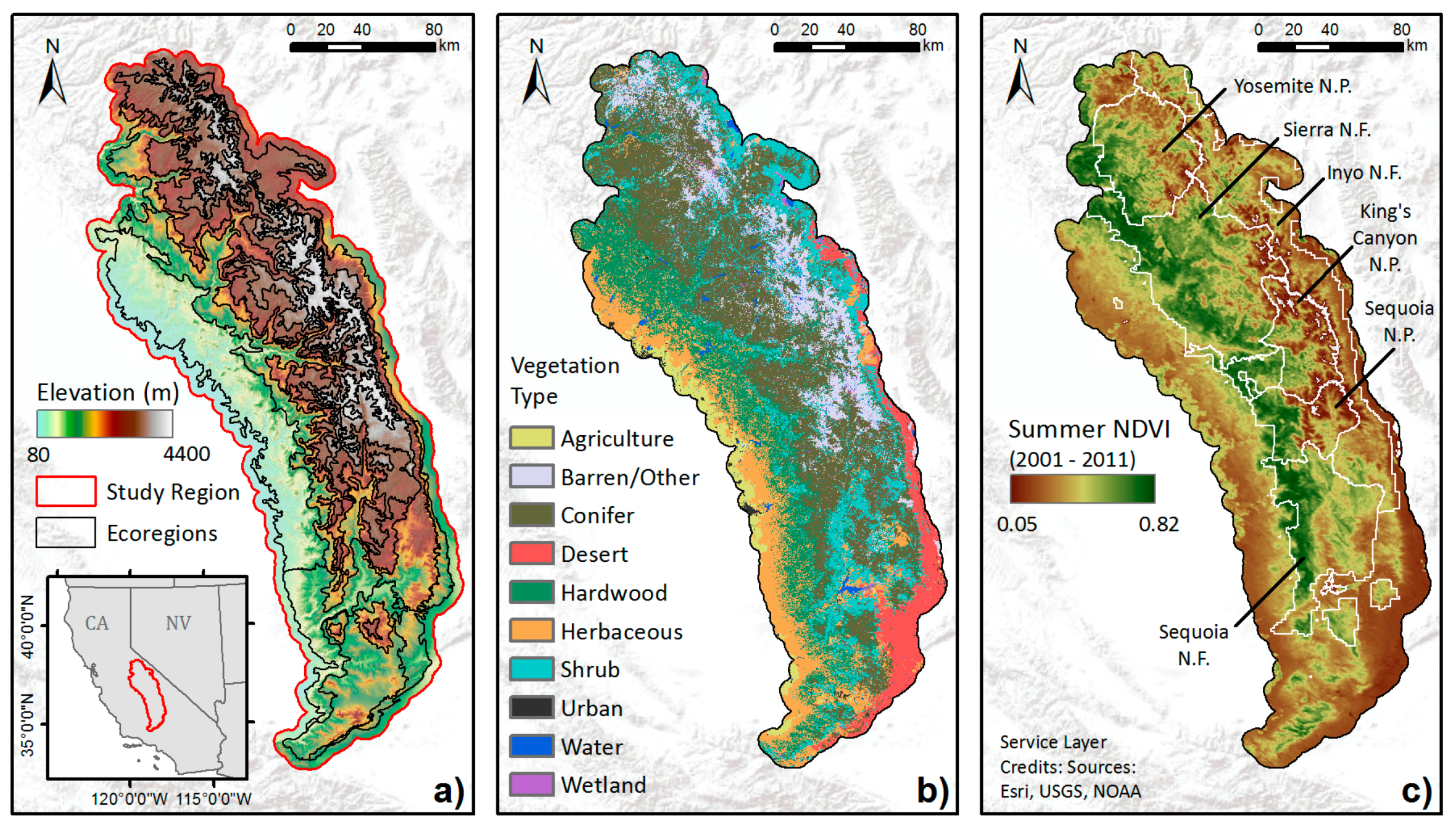
Figure 2.
Cumulative observations of tree mortality parcels with ≥1 dead tree per acre in Central and Southern Sierra Nevada from 2011 to 2016. The inset shows the location of example pixels with different levels of tree mortality as described in Section 3.1.1: one with observed mortality according to the ADS (25 dead trees per acre), the other with no observed mortality that serves as a control sample.
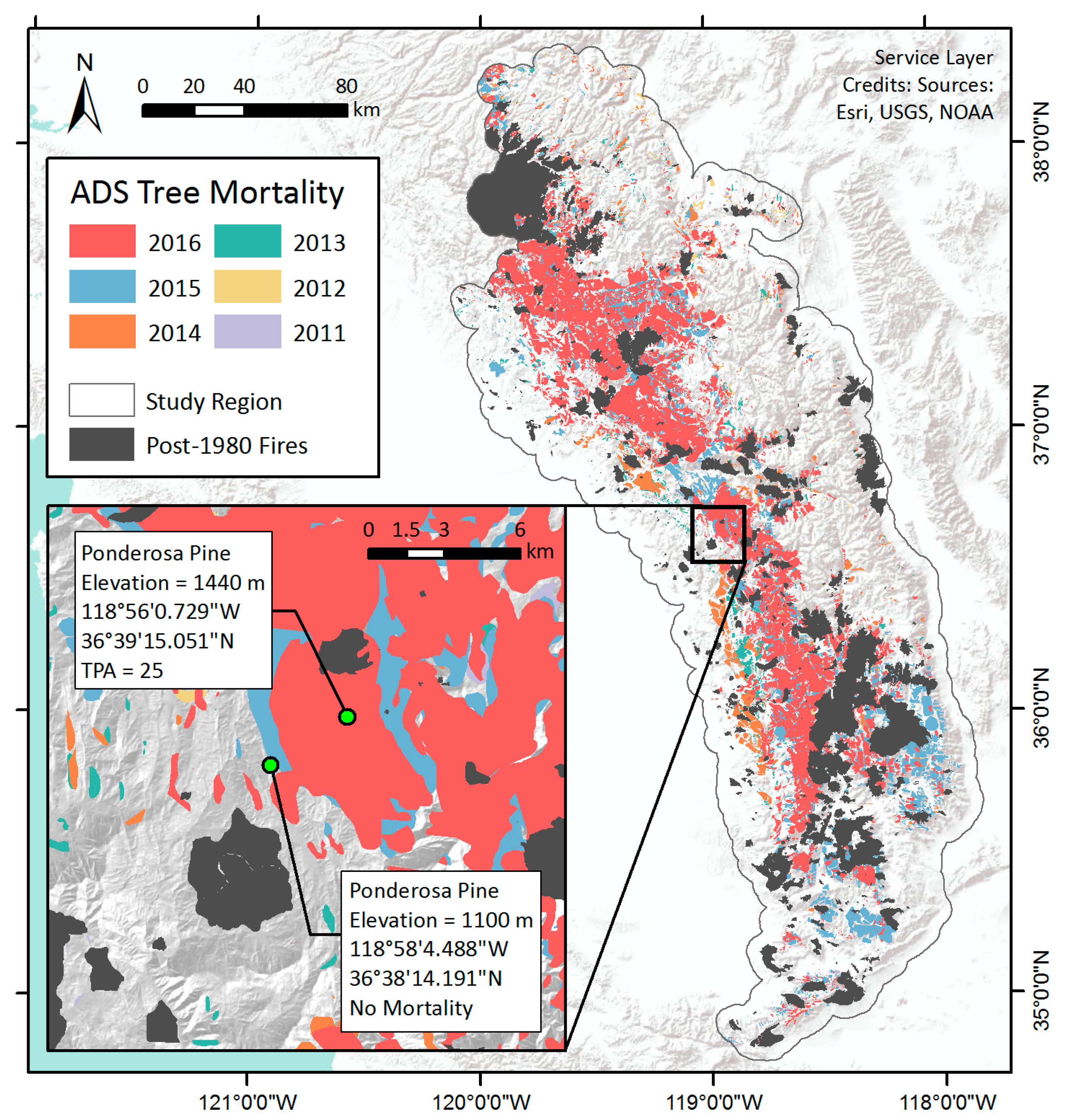
Figure 3.
Progression of tree mortality in the study region, as shown by annual areas of observed tree mortality by severity class, based on the number of dead trees per acre (TPA) in the ADS data. Total flown areas were similar across years, ranging from 6.5 million acres in 2015 to 7.9 million acres in 2016.
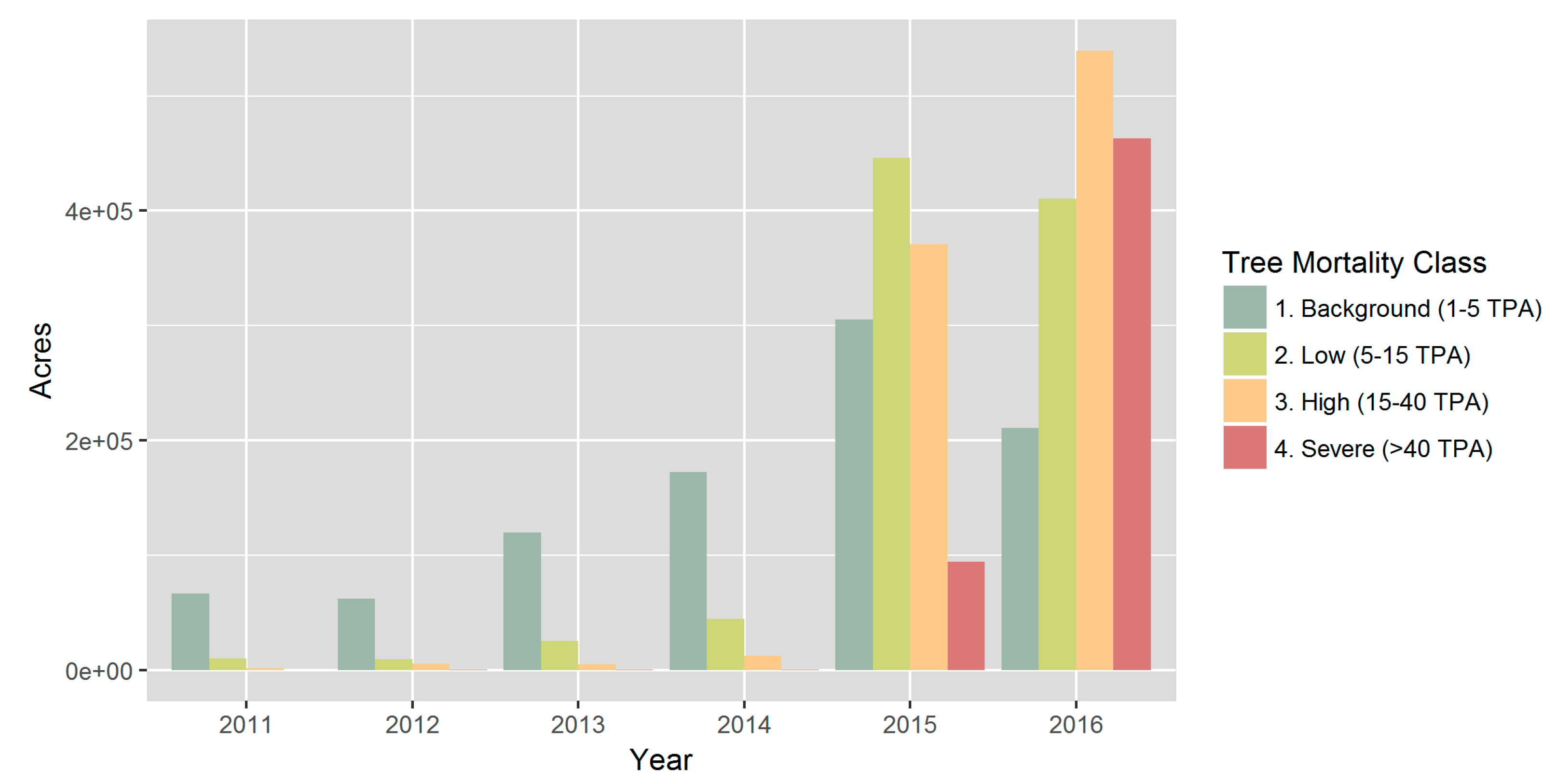
Figure 4.
Temporal dynamics of NDVI over two example Ponderosa Pine pixels, as shown in Figure 2, one with severe mortality (a,b) and the other without mortality (c,d) according to the 2016 ADS survey. In the left panel (a,c), Multi-year mean phenology of NDVI from 2001–2011 is shown in black, with ±2 standard deviations shaded in gray, and annual NDVI time series for each individual drought year from 2013 to 2016 shown in colors. Right panel (b,d) shows interannual variation of late summer NDVI in black, with corresponding z-score on the right vertical axis; Also shown are baseline late summer NDVI (dashed) with ±2 standard deviation (shaded) and NDVI trends over three time periods: β baseline (2001–2011); β drought (2012–2016); β all year (2001–2016).

Figure 5.
Regional 2016 class statistics of (a) summer NDVI z-score, (b) baseline NDVI, (c) EVI trend during the drought period (βdrought), and (d) NDWI trend during the baseline period (βbaseline), summarized for each tree mortality severity class based on the 2016 ADS map of dead trees per acre (TPA). Median values for each class are marked by the central horizontal black line, and mean values are marked by the horizontal dashed line. The end of each whisker marks the upper and lower 10th quantile of each class.

Figure 6.
Distributions of tree mortality severity classes based on the 2016 map of dead trees per acre (TPA) from Reference ADS data (green), and from the one-stage CRF (red) and two-stage CRF predictions (blue).
Figure 6.
Distributions of tree mortality severity classes based on the 2016 map of dead trees per acre (TPA) from Reference ADS data (green), and from the one-stage CRF (red) and two-stage CRF predictions (blue).

Figure 7.
Histogram distributions of dead trees per acre (TPA) within the validation datasets for (a) the mortality-only RRF TPA estimates (blue) vs. reference TPA ≥ 5 (green), and (b) the one-stage RRF TPA estimates.
Figure 7.
Histogram distributions of dead trees per acre (TPA) within the validation datasets for (a) the mortality-only RRF TPA estimates (blue) vs. reference TPA ≥ 5 (green), and (b) the one-stage RRF TPA estimates.

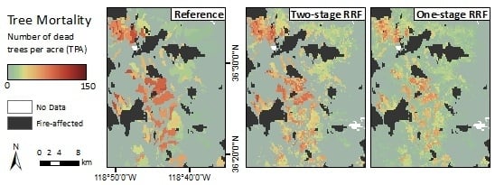
Figure 8.
Mapped 2016 tree mortality classes from the Reference ADS layer (left), two-stage CRF (middle), and one-stage CRF (right) across the whole study region and within two zoomed extents. The modeled maps have missing data in the highest elevations and over water bodies where remote sensing-derived metrics were not available due to the QA process.

Figure 9.
Maps of dead trees per acre from the Reference ADS layer (left), two-stage RRF (middle), and one-stage RRF (right) across the whole study region and within two zoomed extents.
Figure 9.
Maps of dead trees per acre from the Reference ADS layer (left), two-stage RRF (middle), and one-stage RRF (right) across the whole study region and within two zoomed extents.
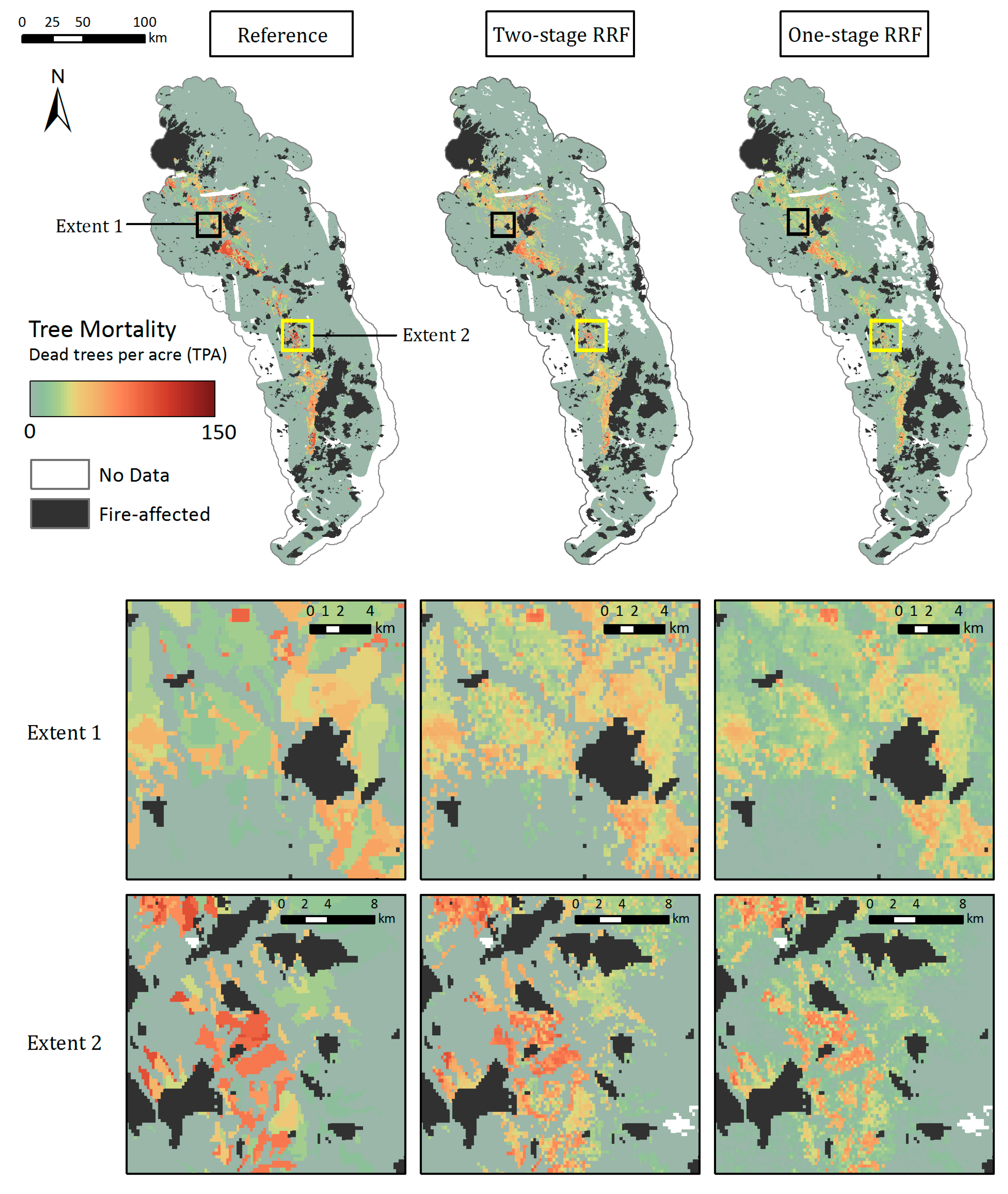
Figure 10.
Variable importance plots from the Binary CRF (a) and Mortality-only CRF (b). Variables further to the left (a greater decrease in Gini Index) are considered more important for minimizing classification error.
Figure 10.
Variable importance plots from the Binary CRF (a) and Mortality-only CRF (b). Variables further to the left (a greater decrease in Gini Index) are considered more important for minimizing classification error.
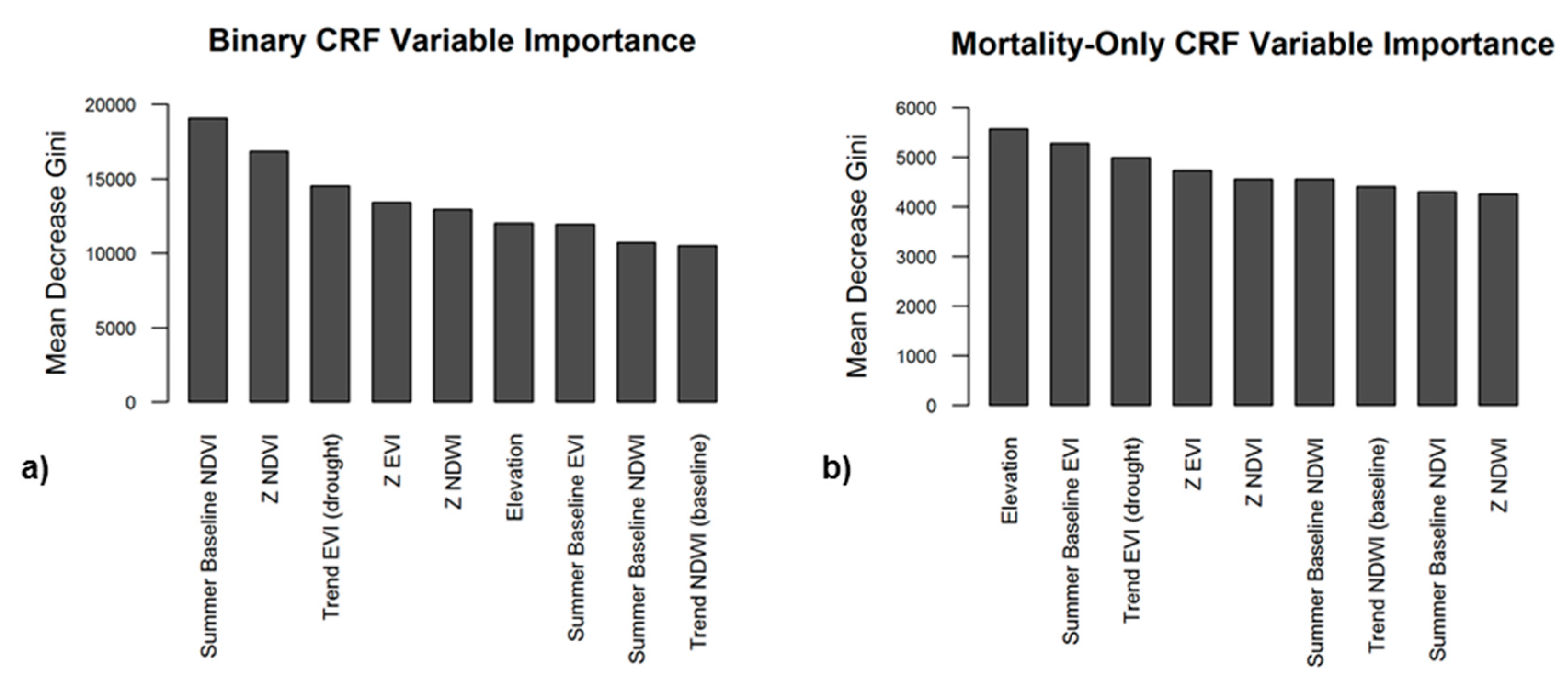
Figure 11.
Partial dependence of dead trees per acre on elevation from the mortality-only RRF model.
Figure 11.
Partial dependence of dead trees per acre on elevation from the mortality-only RRF model.
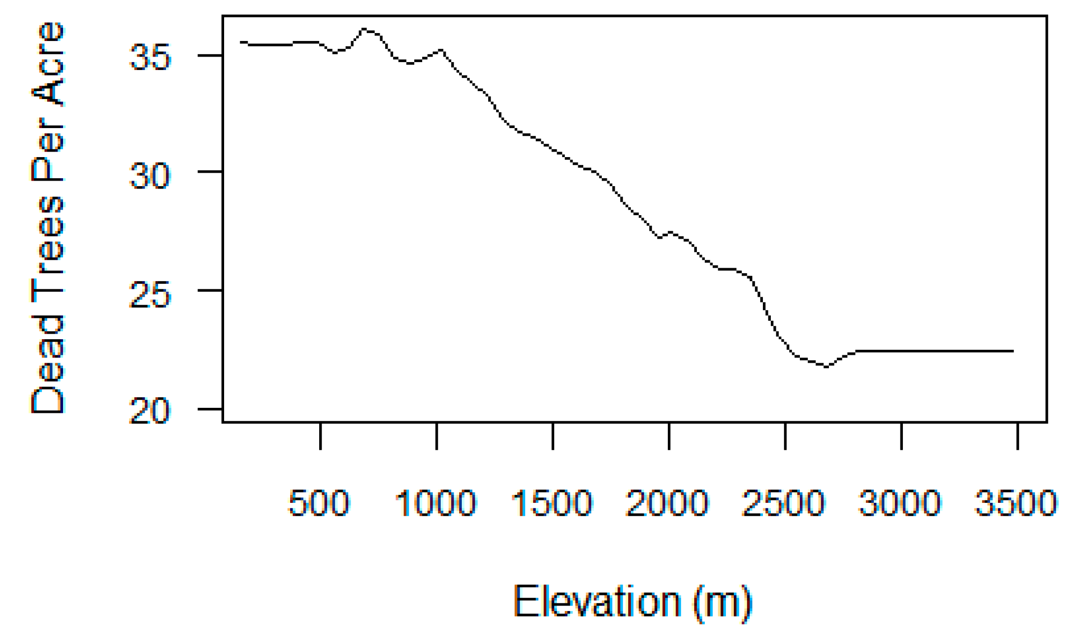

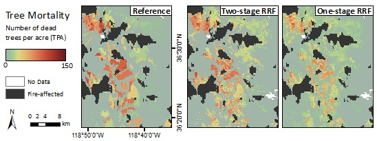
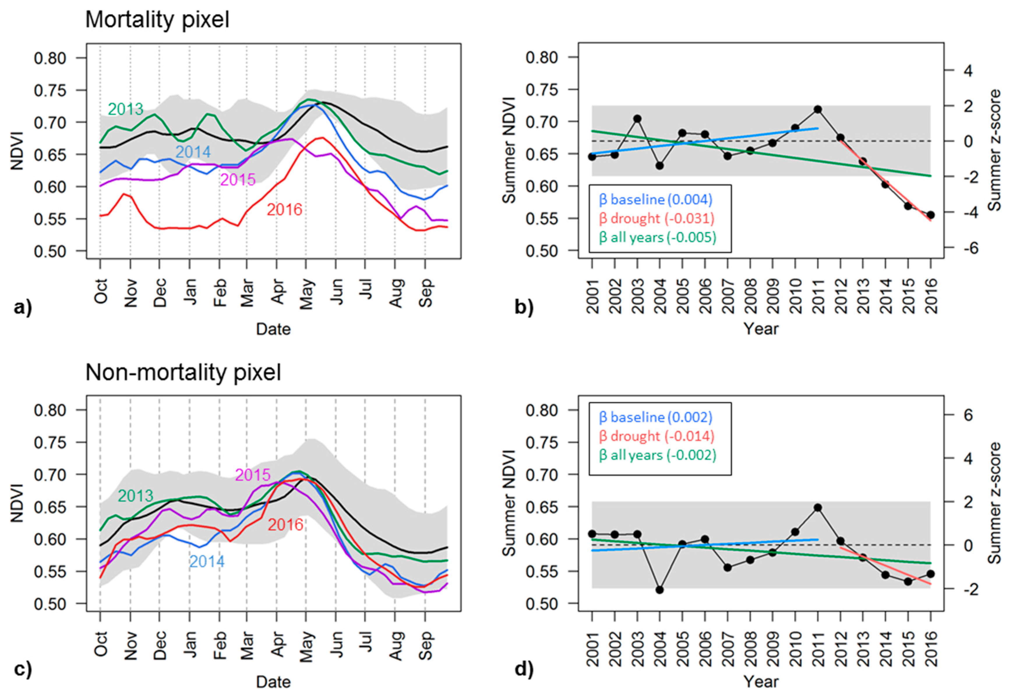
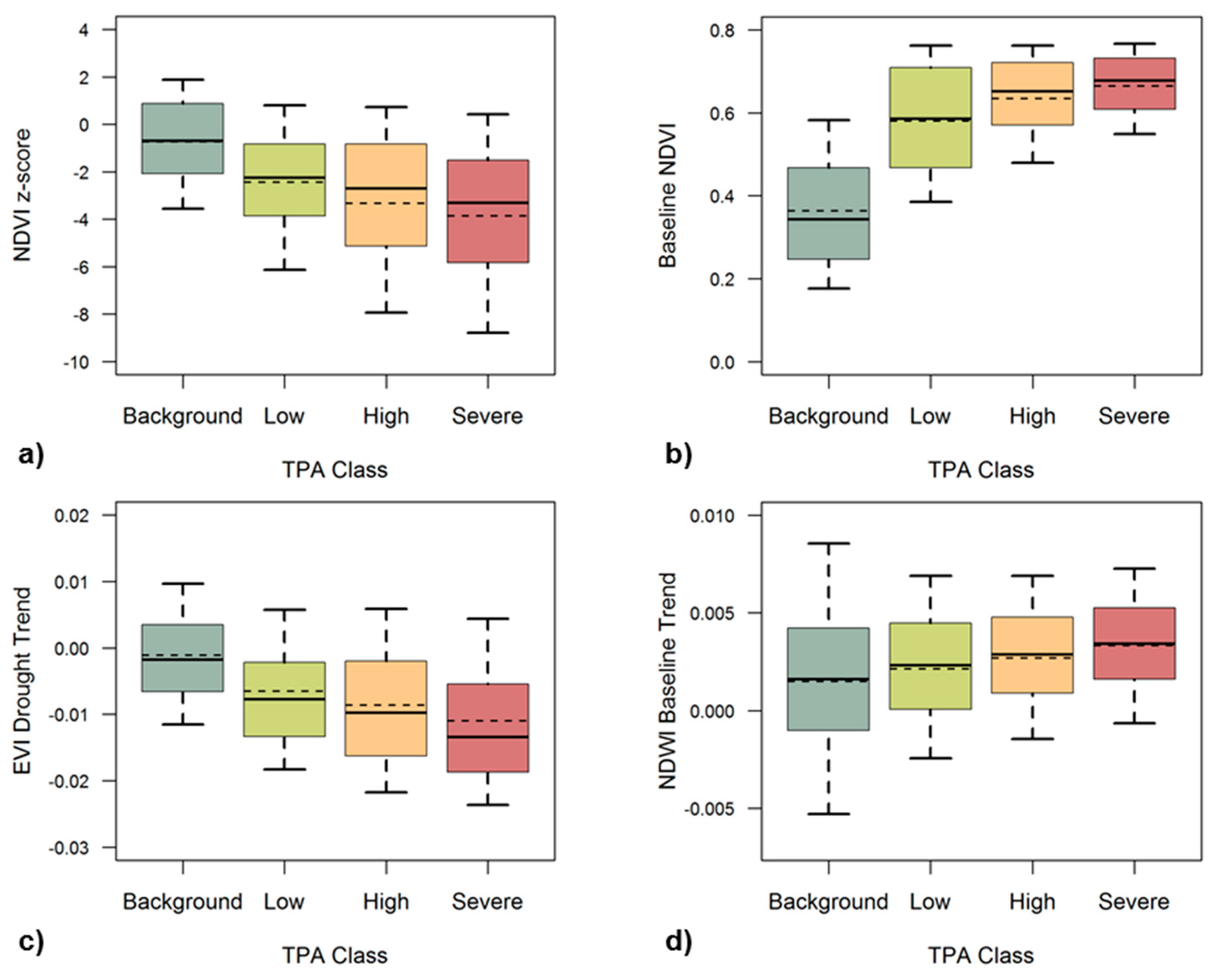
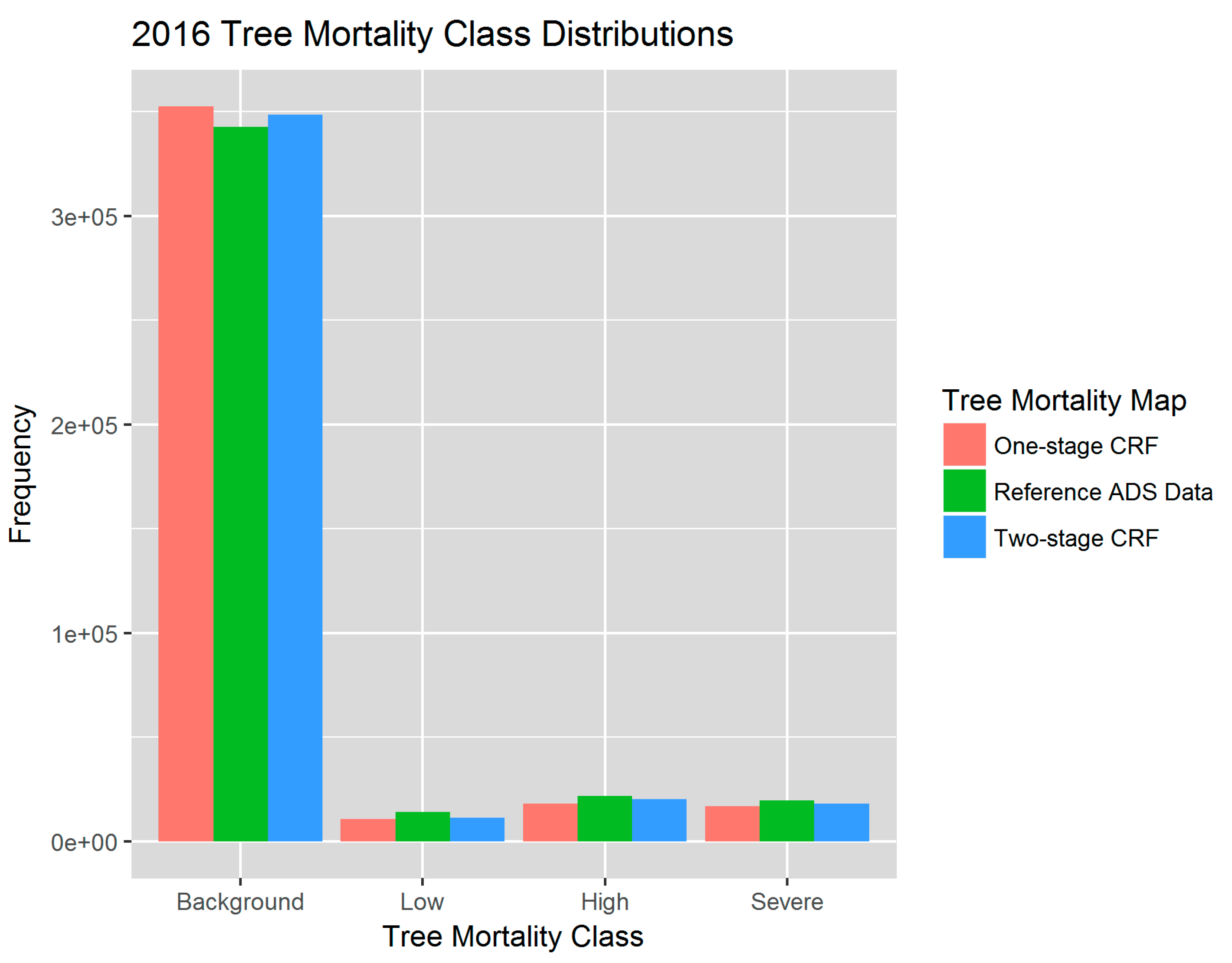
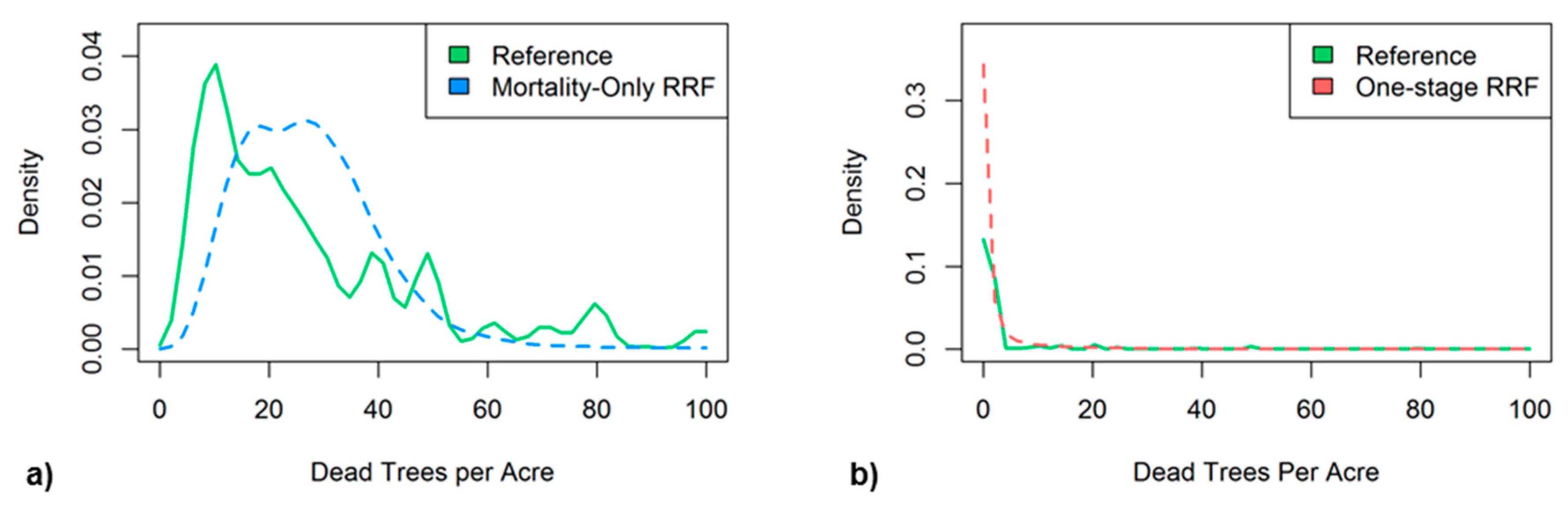
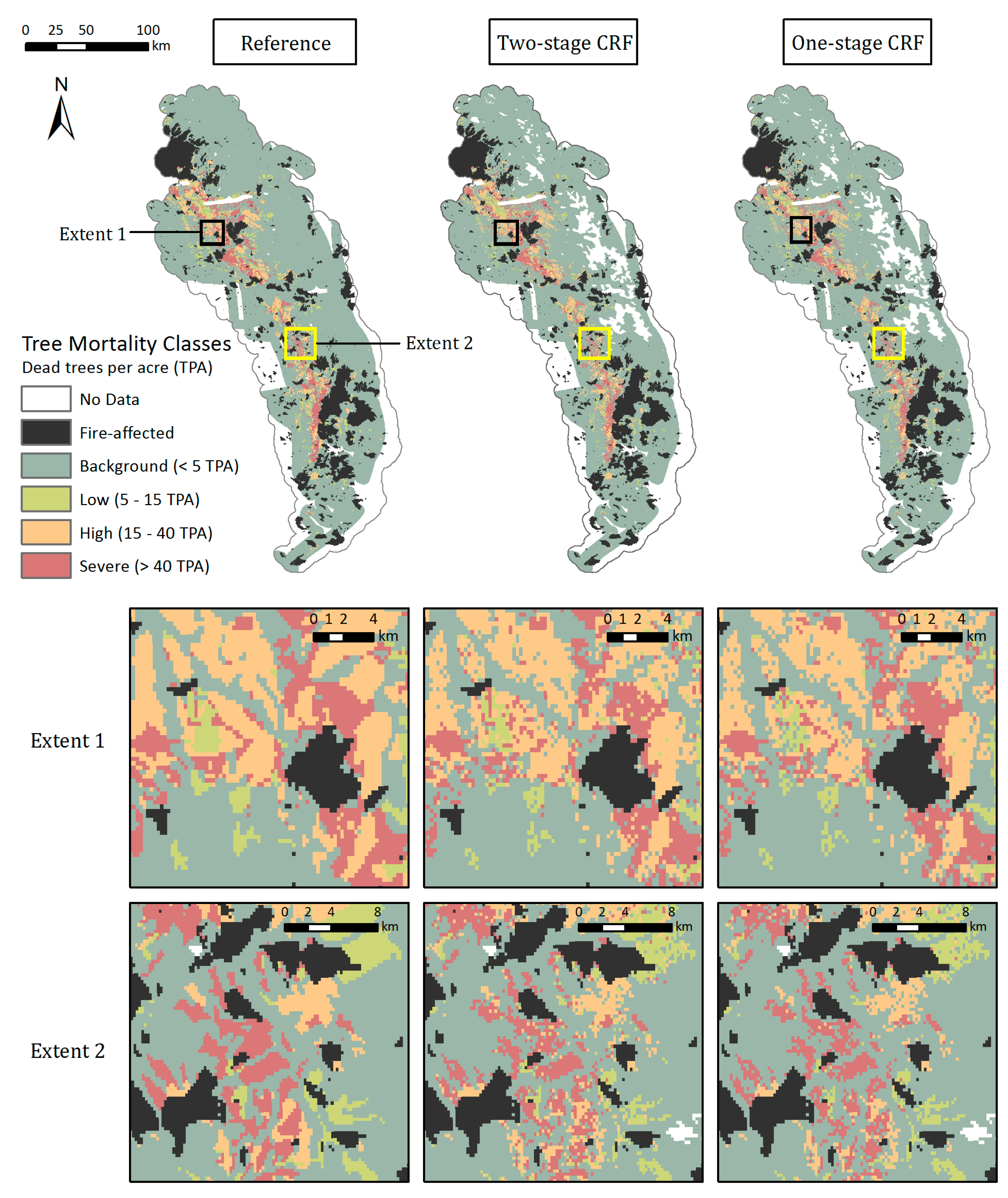
Table 1.
Confusion matrix for the binary classification random forest (CRF) based on the validation data, showing the number and percentage of correctly classified pixels into the background or significant tree mortality classes.
Table 1.
Confusion matrix for the binary classification random forest (CRF) based on the validation data, showing the number and percentage of correctly classified pixels into the background or significant tree mortality classes.
| Predicted Mortality | Reference Mortality | Consumer’s Accuracy (%) | Comission Error (%) | |
|---|---|---|---|---|
| Background | Significant | |||
| Background | 411,746 | 16,266 | 96.2 | 3.8 |
| Significant | 3635 | 11,520 | 76.0 | 24.0 |
| Producer’s Accuracy (%) | 99.1 | 41.5 | ||
| Omission Error (%) | 0.9 | 58.5 | ||
| Overall Accuracy (%) | 95.5 | |||
Table 2.
Confusion matrix for the mortality-only classification random forest (CRF) based on the validation data, showing the number and percentage of correctly classified pixels into the low, high, or severe mortality classes.
Table 2.
Confusion matrix for the mortality-only classification random forest (CRF) based on the validation data, showing the number and percentage of correctly classified pixels into the low, high, or severe mortality classes.
| Predicted Mortality | Reference Mortality | Consumer’s Accuracy (%) | Commission Error (%) | ||
|---|---|---|---|---|---|
| Low | High | Severe | |||
| Low | 7708 | 1558 | 619 | 78.0 | 22.0 |
| High | 1429 | 8317 | 1673 | 72.8 | 27.2 |
| Severe | 589 | 1067 | 4929 | 74.9 | 25.1 |
| Producer’s Accuracy (%) | 79.3 | 76.0 | 68.3 | ||
| Omission Error (%) | 20.7 | 24.0 | 31.7 | ||
| Overall Accuracy (%) | 75.1 | ||||
Table 3.
Confusion matrix for the final two-stage CRF based on the 2016 map data, showing the number and percentage of correctly classified pixels into each tree mortality class, with the area weighted overall accuracy.
Table 3.
Confusion matrix for the final two-stage CRF based on the 2016 map data, showing the number and percentage of correctly classified pixels into each tree mortality class, with the area weighted overall accuracy.
| Predicted Mortality Class | Reference Mortality Class | Consumer’s Accuracy (%) | Commission Error (%) | |||
|---|---|---|---|---|---|---|
| Background | Low | High | Severe | |||
| Background | 340,419 | 2824 | 3042 | 2275 | 97.7 | 2.3 |
| Low | 245 | 10,282 | 567 | 359 | 89.8 | 10.2 |
| High | 1167 | 691 | 17,269 | 1227 | 84.8 | 15.2 |
| Severe | 641 | 383 | 847 | 15,958 | 88.0 | 12.0 |
| Producer’s Accuracy (%) | 99.3 | 72.5 | 79.5 | 80.5 | ||
| Omission Error (%) | 0.7 | 27.5 | 20.5 | 19.5 | ||
| Overall Accuracy (%) | 96.3 | |||||
| Area Weighted Overall Accuracy (%) | 96.2 | |||||
© 2017 by the authors. Licensee MDPI, Basel, Switzerland. This article is an open access article distributed under the terms and conditions of the Creative Commons Attribution (CC BY) license (http://creativecommons.org/licenses/by/4.0/).
Share and Cite
MDPI and ACS Style
Byer, S.; Jin, Y. Detecting Drought-Induced Tree Mortality in Sierra Nevada Forests with Time Series of Satellite Data. Remote Sens. 2017, 9, 929. https://doi.org/10.3390/rs9090929
AMA Style
Byer S, Jin Y. Detecting Drought-Induced Tree Mortality in Sierra Nevada Forests with Time Series of Satellite Data. Remote Sensing. 2017; 9(9):929. https://doi.org/10.3390/rs9090929
Chicago/Turabian StyleByer, Sarah, and Yufang Jin. 2017. "Detecting Drought-Induced Tree Mortality in Sierra Nevada Forests with Time Series of Satellite Data" Remote Sensing 9, no. 9: 929. https://doi.org/10.3390/rs9090929
Note that from the first issue of 2016, this journal uses article numbers instead of page numbers. See further details here.