Hindcasting and Forecasting of Surface Flow Fields through Assimilating High Frequency Remotely Sensing Radar Data


1
Department of Civil Engineering, National University of Ireland Galway, H91 TK33 Galway, Ireland
2
Ryan Institute, H91 TK33 Galway, Ireland
*
Author to whom correspondence should be addressed.
Remote Sens. 2017, 9(9), 932; https://doi.org/10.3390/rs9090932
Submission received: 4 July 2017
/
Revised: 24 August 2017
/
Accepted: 6 September 2017
/
Published: 8 September 2017
(This article belongs to the Special Issue Radar Remote Sensing of Oceans and Coastal Areas)
Abstract
:In order to improve the forecasting ability of numerical models, a sequential data assimilation scheme, nudging, was applied to blend remotely sensing high-frequency (HF) radar surface currents with results from a three-dimensional numerical, EFDC (Environmental Fluid Dynamics Code) model. For the first time, this research presents the most appropriate nudging parameters, which were determined from sensitivity experiments. To examine the influence of data assimilation cycle lengths on forecasts and to extend forecasting improvements, the duration of data assimilation cycles was studied through assimilating linearly interpolated temporal radar data. Data assimilation nudging parameters have not been previously analyzed. Assimilation of HF radar measurements at each model computational timestep outperformed those assimilation models using longer data assimilation cycle lengths; root-mean-square error (RMSE) values of both surface velocity components during a 12 h model forecasting period indicated that surface flow fields were significantly improved when implementing nudging assimilation at each model computational timestep. The Data Assimilation Skill Score (DASS) technique was used to quantitatively evaluate forecast improvements. The averaged values of DASS over the data assimilation domain were 26% and 33% for east–west and north–south velocity components, respectively, over the half-day forecasting period. Correlation of Averaged Kinetic Energy (AKE) was improved by more than 10% in the best data assimilation model. Time series of velocity components and surface flow fields were presented to illustrate the improvement resulting from data assimilation application over time.
Keywords:
remote sensing; nudging; data assimilation; surface currents; CODAR; forecasting; hindcasting; Galway Bay; radars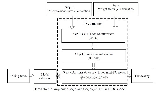
1. Introduction
Accurate forecasting of surface currents in coastal areas is of great importance for operations such as search and rescue, fishing, and pollution monitoring. There are generally three main approaches to determine dynamic processes of coastal waters: observations, scaled physical modelling, and numerical modelling. Each of these provides meaningful information to analyze dynamic processes of relevant phenomena. However, each approach has its own constraints and shortcomings. Observations based on remote sensing are a desirable way to obtain data of real states, but they are usually expensive. Moreover, observation biases from observers or measurement tools can reduce the reliability of recorded data. Scaled physical experimentation is a useful way to investigate variations of dynamic processes, but such experiments are usually time-consuming and expensive to perform. In addition, limitations exist when extrapolating data obtained from a scaled model to a prototype, such as scaling, friction, and viscosity; experimental errors are also inevitable. Accurate definition of initial conditions, boundary conditions, constitutive relations, and external forcing, among others, is not easy in numerical modelling. Since changing processes of dynamics of interest in nature are continuous and complex, the artificial definition of temporal and spatial resolution overly simplifies internal processes in numerical models. Some assumptions and approximations can also cause significant errors in numerical models. With the development of advanced measuring techniques, such as radar and satellite, based on remote sensing technologies, significant hydrodynamic data can now be obtained for coastal waters. Although accurate numerical modelling is difficult to set up, it is an efficient and powerful tool to inform about dynamic processes due to its low cost and easy operation, compared with observations and scaled physical experiments. Additionally, numerical models can produce forecast information at a relatively low cost, once a model is established.
In order to best utilize the above methods for improved simulation (both hindcasting and forecasting), a blending of useful and reliable information from measurements, and physical experiments with numerical model results, has been broadly developed. This blending process, called data assimilation, has been applied in atmospheric modelling for a few decades, and currently is becoming more widely used in oceanography, due to increased monitoring of oceanic data in space and time. There are two main types of data assimilation schemes: sequential and variational [1,2]. The analysis equation of a sequential data assimilation scheme is obtained by a linear combination of measurement states and model background states, such as nudging, optimum interpolation (OI) and Ensemble Kalman Filter (EnKF) [3,4,5]. The analysis equation of a variational data assimilation scheme is derived by minimizing a cost function, which is made up of two terms: one is the distance between the analysis states and the model background states; the other is the distance between the analysis states and the observation states [6]. Three-dimensional variational (3D-VAR) data assimilation and four-dimensional variational (4D-VAR) data assimilation are examples of advanced variational data assimilation solvers [7,8,9,10,11].
Sequential data assimilation algorithms, such as nudging and OI, are now being employed in oceanography to synthesize measurements into models. A number of researchers previously assimilated HF radar data to improve the surface currents model forecasts using sequential data assimilation schemes. Paduan and Shulman [12] assimilated HF radar data into a model of Monterey Bay via correcting wind forcing based on physical principle, i.e., conservation of energy or Ekman theory. They found that a significant improvement in the correction between the model and observed subsurface current was achieved when an Ekman-layer projection of the correction was included. Ren et al. [13] also used a similar data assimilation approach to correct the wind stress in a three-dimensional model for Galway Bay using the HF radar surface currents. Results indicated that both velocity components were considerably improved during the forecasting period. Their results showed that improvements of root-mean-square error (RMSE) for direction of surface flow fields were significant. Barth et al. [14] assimilated HF radar currents in a West Florida Shelf (WFS) model based on the Regional Ocean Model System (ROMS) using Kalman Filter theory. Error covariances were estimated from an ensemble simulation of the WFS model results, using different wind forcing. Results of the WFS model assimilating HF radar currents showed an improvement of the model current results, not only at the surface but also at depth. Breivik and Satra [15] developed a real-time system assimilating HF radar currents into their model with an improved OI scheme. Spatial covariance, derived from their ocean model, was used instead of simplified mathematical formulations. Results showed that both analyses and forecasts outperformed results from a model not using data assimilation (“free run”). However, the six-hour forecast from the assimilation model was only marginally better than the “free run”. They also found that the relatively weak cross-correlations observed between modelled results and the hydrography discouraged the use of an OI approach.
Weighting factors in nudging algorithms are analytically prescribed, rather than obtained from covariances; model background error covariance and measure error covariance are not required. Hence, the nudging data assimilation technique is becoming a popular approach in assimilating oceanic measurements into models, due to its easy implementation and low computational cost.
Fan et al. [16] assimilated drifter and satellite data into a circulation model with a nudging algorithm for the Northeastern Gulf of Mexico. They compared the results from models with and without data assimilation. Comparisons of the modeled currents with moored data on the West Florida Shelf showed that data assimilation improved modelling performance. Fan, Oey, and Hamilton [16], found that drifter position errors ranged from 30 to 80 km with a mean of about 60 km over 10-day periods, which were comparable to errors obtained by Castellari et al. [17].
Lin et al. [18] also applied a nudging data assimilation scheme to quantify the accuracy of currents in an eddy-rich ocean environment, using altimetry sea-surface height anomaly (SSHA) and surface drifter data. Their results showed that combined altimetry SSHA and drifter analysis consistently outperformed analyses in which altimetry sea-surface height anomaly alone was assimilated. In particular, they found that assimilation of drifter data can generate small-scale eddies that were generally not resolved by satellite data. Additionally, employment of data assimilation techniques for shelf study over the deep ocean region can result in better boundary conditions for shelf hydrodynamic models.
Gopalakrishnan and Blumberg [5] also assimilated HF radar data into an estuarine and coastal ocean circulation model using a nudging data assimilation algorithm. They introduced a nudging parameter into the equations of motion which affected the model dynamics. The HF radar data were imparted to neighboring grid points via model dynamics. The impacts of the data assimilation undertaken were analyzed by running models, with and without data assimilation. Data Assimilation Skill Score (DASS) based on mean-square error (MSE) was computed to assess the improvement of forecasting with nudging data assimilation algorithm in their research. Their results showed that the nudging data assimilation scheme was robust and efficient for assimilating the HF radar data into a three-dimensional operational forecasting model. The value of DASS was 18% and 7% for east–west and north–south surface velocity components, respectively, during a one-day forecasting period. This indicated that assimilation of HF radar data with a nudging scheme significantly enhanced both velocity components during the forecasting period, and was a simple yet promising approach to improve model performance.
Available observation data are an essential component when establishing a data assimilation system. A Coastal Ocean Dynamics Applications Radar (CODAR) system has been deployed in Galway Bay located at the west coast of Ireland, since 2011. High density surface currents in this area are captured hourly by this system. Variations in surface currents in Galway Bay area are mainly wind-induced [19,20]. Consistent offshore wind records are difficult to obtain, and model errors for this area mainly result from inaccurate wind forcing data.
In this paper, in order to investigate the surface flow fields for the wind-dominated domain and to improve modelling capability for both hindcasting and forecasting, the nudging data assimilation algorithm was applied to combine HF radar surface velocity components within a three-dimensional numerical model. Nudging data assimilation relies on a few empirical parameters, and no research has been performed to date investigating changes in the nudging parameters on the sensitivity of data assimilation results. This was investigated here, and was an important and novel contribution. Firstly, nudging parameters were examined through assimilating hourly radar data into models. Appropriate nudging parameters were selected based on obtaining minimum RMSE values of surface velocity component(s) between model analysis states and radar observations. Secondly, sensitivity tests on data assimilation cycle length were performed to improve modelling accuracy based on properties of radar data. Results of data assimilation models with different cycle lengths were compared and assessed based on skill scores: DASS, Averaged Kinetic Energy (AKE), visual display of time series, and surface flow fields. The best data assimilation model using nudging algorithm for Galway Bay, was then chosen based on a comprehensive assessment.
An outline of the reminder of this paper is: Section 2 gives a brief description about the Galway Bay HF radar system, the numerical model developed, and the nudging data assimilation algorithm. Sensitivity experiments of nudging parameters and data assimilation cycle lengths are described in detail in Section 3, followed by results from the nudging data assimilation models in Section 4. A discussion is presented in Section 5, and conclusions are presented in Section 6.
2. Methodologies
2.1. High Frequency Radar System
Remote sensing is a technology to obtain information about objects or areas from a distance, usually based on radars, aircraft, or satellites. Remote sensing observations have a wide range of coastal applications, such as monitor ocean circulation and current systems, sea ice tracking, and mapping of coastal features. Ocean data collected by remote sensing can be used to better understand the oceans, to provide knowledge to best manage ocean resources, and to provide useful, accurate information for commercial and recreational applications. CODAR is a land-based HF remotely sensing radar system which measures the near-surface ocean currents in a coastal area with fine temporal and spatial resolutions. One such system, consisting of two radar masts, was deployed on Galway Bay (see Figure 1) in 2011. This system is capable of monitoring the surface currents and wave parameters over most of inner Galway Bay. Measurements obtained from the CODAR system are in near real time. When a radar signal scatters off a wave whose wave length is exactly equal to half of the transmitted signal wavelength, the radar signal can return measurement information to the radar receiver [21,22,23]. A single HF radar station determines radial components of surface currents toward and away from that station. Total surface currents are computed and displayed as vector fields, by combining the radial surface current velocity components from two or more different masts [24,25].
Shulman and Paduan [26] assimilated 33-h low-pass-filtered radar data and unfiltered radar data into a model for the Monterey Bay area using OI; they found good agreement with moored current observations. Moreover, they assimilated radial and total surface currents separately. Results indicated that assimilation of radial surface currents extended the range of influence of the data into regions covered by only one HF radar site. Since the authors focused on enhancing the surface flow fields in the whole inner Galway Bay area, the unfiltered total vector fields with larger spatial coverage were employed to build a data assimilation forecasting system using nudging data assimilation technique in this work.
The CODAR system provides rich datasets in time and space. They can be used to explore the dynamical process of surface currents, to implement data assimilation and to validate numerical models [27,28,29]. The temporal and spatial resolutions of surface currents in the Galway Bay domain are sixty minutes and 300 m, respectively. The operating frequency of both radar stations in Galway Bay at C1 and C2, as shown in Figure 1, is 25 MHz. Advantages of remote sensing CODAR system over the conventional techniques include: synoptic coverage, repeated observations and high temporal and spatial resolution.
Although data transfer delay usually exists when processing radar results, it is less than one hour in the case of the Galway Bay CODAR system. In addition, radar data were not assimilated into models during forecasting periods. Once the data assimilation model was developed, the model can be employed to produce actual forecasts.
2.2. Numerical Model
The numerical model, EFDC, was used to simulate the hydrodynamic circulation of Galway Bay. EFDC was developed at the Virginia Institute of Marine Science by the U.S. Environmental Protection Agency (EPA). It comprises four linked modules: hydrodynamic, water quality and eutrophication, sediment transport, and toxic chemical transport and fate. Only the hydrodynamic module was used during this research. This module solves the three-dimensional, vertically hydrostatic, free surface, turbulent averaged equations of motion for a variable density fluid. The hydrodynamic component of EFDC uses a semi-implicit, conservative finite volume solution scheme for the hydrostatic primitive equations, with either two or three level timestepping [30,31,32]. The model uses a sigma vertical coordinate system, and either regular, or curvilinear orthogonal horizontal coordinates. The model had been applied to a variety of modelling studies of rivers, lakes, estuaries, and coastal regions [33,34,35].
The dynamics within Galway Bay are dominated by oceanic flows into the bay from the Atlantic shelf and wind driven currents. Oceanic flows enter and exit the bay mainly through the sounds around the Aran Islands. Meteorological parameters are strongly affected by the Atlantic weather system [36]. The main wind direction in this area is southwest [37]. In this research, a barotropic model of Galway Bay (see Figure 1) was developed using a regular grid coordinate system; a 150 m horizontal spatial resolution was employed, yielding 380 × 241 grid cells. Variable vertical layer thicknesses were used in the model, with a thinner layer at the top and bottom of the water column, and thicker layers in the middle, thereby ensuring that wind forcing was not overly-damped by tidal forcing. A detailed description on setting up vertical layer structure for the Galway Bay can be found in the study by Ren et al. [38]. The meteorological forcing data (wind, pressure, rain, solar radiation, and relative humidity) were obtained at one minute intervals from the Informatics Research Unit for Sustainable Engineering (IRUSE) weather station located at the campus of National University of Ireland, Galway. Records of the River Corrib inflows, which enter Galway Bay close to the north of point C1 in Figure 1, were obtained from the Irish Office of Public Works (OPW). Tidal water elevation time series generated from Oregon State University Tidal Inversion Software (OTIS) were used to define the tidal forcing on the western and southern open boundaries (see Figure 1) in the model [39,40].
The simulation period was from Julian Day 211 to 230 in 2013; this period was subdivided as follows: (i) spin-up period, Julian Day 211–220; (ii) data assimilation period, Julian Day 220–228 01:00; (iii) forecasting period, after Julian Day 228 01:00. During this simulation period, the measured radar data have high density in time and space.
2.3. Data Assimilation
Nudging is a sequential data assimilation algorithm that combines model background states with measurement states in a linear formula. Model background states were calculated from surface velocity components from the EFDC model. A nudging term was introduced into the equations of motion using the difference between model background states and observation states [5]. The analysis equation has been conceptually expressed as [41]:
where is the model background states; is the observation states from radars; is the nudging parameter; (physics) denotes the physical process mathematically described in the numerical model.
The nudging parameter is defined in the following empirical equation [41]:
where is the distance between model grid point and the observation data location; is the difference between assimilation and observation time; is an assimilation timescale, which determines the strength of the nudging parameter; is a damping time scale for the nudging term; is a nudging length scale; is the exponential decay parameter, which controls the depth of influence of the nudging parameter; is the water depth (m); is the depth of influence (m).
Nudging algorithms are approximations of the OI data assimilation scheme; the main differences lie in that the Kalman gain used in the OI algorithm is substituted by the nudging parameter.
In this research, surface currents measured by the HF radar system were assimilated into the EFDC model using the nudging data assimilation algorithm. Houser et al. [42] found that better results were obtained through nudging towards a gridded analysis using spatially interpolated precipitation data into a hydrologic model, compared to others. Rusu and Guedes Soares [43] found that the accuracy of predictions was enhanced as the amount of the data assimilated increased. Moreover, in order to ensure consistency between model background states and measurements in space during the data assimilation process, nudging towards a gridded analysis presented by Stauffer and Seaman [44] was applied in this research through spatially bilinearly interpolating radar data onto model grid points. Because the spatially interpolated HF radar measurements were collocated with the model grid point and were linearly interpolated over time to every assimilation timestep, and . indicated that the model grid and the observational location remained the same, and indicated that there was no time-lag between the model simulation and measurements. Thus, the nudging parameter can be simplified to:
The nudging parameter was set to zero at all grid points where HF radar observations were not available. The above expression of nudging parameter, , was used by Gopalakrishnan and Blumberg [5].
2.4. Implementation of Data Assimilation
A complete data assimilation system is comprised of three parts: a numerical model, a data assimilation algorithm, and observational data sets. Since the authors focused on simulating the surface currents in Galway Bay, in this research, a subroutine including a nudging data assimilation algorithm was encoded and combined into the EFDC model.
Since surface current vectors are the parameters of primary interest, an overview of the procedure for calculating surface currents in EFDC is shown in Figure 2.
updating of surface flow fields via assimilating radar data using nudging data assimilation was carried out during the process of solving the hydrodynamic equations. HDMT.FOR is the main routine in EFDC used to calculate surface currents, so the assimilation process of radar measurements was incorporated into this routine. However, the hydrodynamic computation within EFDC is quite complex. In order to better show the updating of the surface velocity vectors via assimilating the radar data in the model, the hydrodynamic and mass transport calculation processes in the HDMT.FOR routine was extended and details are presented in Figure 3.
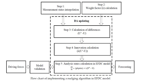
Figure 3 shows general computing process for simulating surface velocity vector in the main program HDTM.FOR. To assimilate the measured surface current data into the model, the shaded subroutine, as shown in Figure 3, was added. Implementation of the data assimilation procedure is presented in Figure 4.
Interpolation of radar data (step 1) and calculation of weight factor () (step 2) were conducted before undertaking data assimilation. Updating of model background states was carried out at each assimilation timestep.
3. Sensitivity Experiments
In order to develop a good data assimilation forecasting model for the Galway Bay domain using the HF radar data, the procedure can be described as a twofold process: firstly, appropriate nudging parameters (assimilation time scale and the depth of influence ) were examined, and appropriate values defined based on RMSE values between surface currents and HF radar data during the hindcasting period. Secondly, sensitivity tests of model forecasts of data assimilation cycle lengths’ influence were undertaken. The authors are not aware of any other such sensitivity analyses that had been carried out to improve model forecasts using nudging data assimilation technique.
3.1. Tests of Nudging Parameters
In order to produce satisfactory results when measurements were assimilated into models using the nudging algorithm, different researchers have used different values of the nudging parameters. For example, Fan et al. [16] set the assimilation scale and the depth of influence of data assimilation as when assimilating drift and satellite data. Lin et al. [18] used the same values of nudging parameters as Fan et al. [16] in their data assimilation system; Gopalakrishnan and Blumberg [5] set values at 1800 s and 2 m, respectively. In this research, assimilation scale and depth of influence were optimized based on more than twenty representative numerical experiments, as presented in Table 1. This was the first time sensitivity analysis had been performed on the parameters of a nudging data assimilation algorithm using radar data. Twenty versions of data assimilation models were run using different values for the nudging parameters. The radar surface currents were assimilated hourly into these test models. Model NDA0, the “free run” with no data assimilated into this model, was used as a benchmark for comparisons.
RMSE between the radar data and the model results were calculated using Equations (4) and (6). RMSE of surface velocity east–west components (u) was firstly calculated with Equations (4) and (5), which average the values of RMSE in space and time; the same equations were used for north–south surface velocity components (v); and the total was finally computed using Equation (6). was used to assess the degree of agreement between modeled results and the HF radar data.
where is the CODAR HF radar measured surface velocity east–west component (cm/s); is the modelled surface velocity east–west component (cm/s); ) is the RMSE of east–west velocity component in space covered by the high frequency radar system at timestep (cm/s); is the number of times using Equation (4); is the number of calculation points at timestep ; is the averaged value of east–west velocity component in space during the data assimilation period (cm/s).
Values of , and over the data assimilation period are presented in Table 1.
Typical variations of the RMSE values in models are presented in Table 1. Other models were examined by the authors as well, but the difference of RMSE values was very small when was greater than 4 m. Averaged between the nudging data assimilation test models, and the HF radar measurements over the data assimilation period, as shown in Table 1, indicated that model results were more sensitive to depth of influence , than the assimilation time scale . Table 1 shows that model NDA10, having the minimum of 10.39 cm/s, generated the best forecast results. It was assumed that good agreements between measurements and modeled results during assimilation period had positive impacts on forecasting. Thus, data assimilation scale and depth of influence of data assimilation as were taken as the best nudging parameters.
To examine the performance of models using the nudging data assimilation algorithm, surface flow fields over the data assimilation period from four representative assimilation models presented in Table 1 were compared with model NDA0 and the radar data in Figure 5.
Figure 5 shows that results from a representative model NDA9 (see Figure 5b) significantly deviated from the HF radar observations; similar deviation occurred when is less than 3 m. This indicated that inappropriate nudging parameters lead to model deviation or even instability. Patterns of surface flow fields in model NDA0, NDA11, and NDA12 were quite similar. Based on averaged surface flow fields during assimilation period, model NDA10 (Figure 5c) can yield closer results to radar data (Figure 5f). In the following studies, the values and were used in nudging data assimilation models.
3.2. Tests of Data Assimilation Cycle Lengths
The temporal resolution of HF radar measurements for Galway Bay domain is sixty minutes. To study the influences of variations in data assimilation cycle lengths on forecasts, and to implement shorter updating of model background states, HF radar data were temporally linearly interpolated onto intervals less than sixty minutes. The reasons for using temporally interpolated radar data are, firstly, Sun [45] suggested that it was desirable to have rapid update cycles to capture the temporal change and to obtain useful information from the model background states. The radar data were not regarded as a single snap-shot by Sun [45], but each point in the three-dimensional data volume was assimilated at the timestep closest to the measurement time in a sequential scan. Secondly, in operational data assimilation forecasting systems, measurements from different resources at different timesteps can be assimilated into models. Thus, assimilation intervals in these models do not have to be at regular time intervals. Application of the temporally interpolated radar measurements is similar to a real forecasting data assimilation case using measurements from different sources. Thirdly, frequent updating using temporally interpolated radar data examines whether or not the three-dimensional coastal EFDC model is sufficiently robust for developing an operational data assimilation model forecasting system. Finally, since hourly output of surface current vectors were obtained by averaging/merging data over a specified time period in the CODAR radar monitoring system, temporal linear interpolation of the output data was somewhat analogous to an inverse process, which conveyed the averaged information to successive timesteps over the measurement period [46]. Linearly interpolated surface velocity data over short periods were assumed to more accurately describe the dynamics of the surface currents.
Since the ultimate goal of using data assimilation techniques was to enhance model performance through optimizing the integration of the measured data, the idea of using linearly interpolated measurements in time, to frequently update the model background states, was a numerical experiment designed to assess the accuracy of forecasted states. Additionally, Ren et al. [47] used constant pseudo measurements to test the influence of data assimilation cycle lengths in the same domain. The results showed that improved surface current forecasting resulted from the assimilation model using shorter updating intervals. It was the first time that linearly interpolated coastal HF surface currents were assimilated into a model to examine modelling performance. Temporal interpolation of radar data was implemented at each observational point where two successive hourly radar measurements were available. Here, five versions of the nudging data assimilation model were developed to assimilate temporally interpolated radar data with different data assimilation cycle lengths: (a) each model computational timestep (MS), (b) one minute, (c) five minutes, (d) fifteen minutes, and (e) sixty minutes. RMSE values were computed and averaged during the +12 h forecasting period (02:00–13:00 Julian Day 228) using Equations (4) and (6). Detailed description of these nudging data assimilation models is given in Table 2. All of the cycle length test models had the same initial and boundary conditions as model NDA10.
Table 2 shows that model NDA21, which updated the model background states at each model computational timestep using the temporally interpolated radar data, showed significant improvements during forecasting period compared with results from model NDA0. Meanwhile, other models updating model background states with longer data assimilation cycle lengths did not change much with respect to forecasting performance in models. Values of RMSE for both surface velocity components in model NDA21 were less than other models with longer data assimilation cycle length. Improvement of averaged RMSE was 10% and 15% for east–west and north–south velocity components separately during a 12-h forecasting period, in comparison with model NDA0.
4. Forecast Assessments of Assimilation Cycle Lengths
The above tests showed that assimilating HF radar data at each model computational timestep can improve surface flow fields using a nudging algorithm. In order to quantitatively and qualitatively compare and assess assimilation model results with the “free run” and radar data, mean surface flow fields from assimilation cycle length test models, “free run” and radar data are presented in Section 4.1. A statistical assessment method, namely DASS, of each surface flow field during a six-hour forecasting period based on MSE, is computed and presented in Section 4.2. Section 4.3 presents an analysis of the correlation of AKE between model results and radar data over a two-day forecasting period. Time series of both surface velocity components’ forecasts from models at one assimilation point are also compared with radar data in Section 4.4.
4.1. Assessment of Mean Surface Flow Fields
An implicit assumption when using data assimilation techniques in numerical models was that a combination of measured data with model background states will improve modelling performance, especially during forecasting periods. In this work, we were interested in enhancing the forecasting of surface flow fields in Galway Bay through assimilating the radar data. In order to explore improvements using a nudging data assimilation algorithm over the domain during a forecast period, averaged surface flow fields during a +12 h forecasting period (start from Julian Day 228, 2013 02:00) were calculated. All nudging data assimilation models had the same conditions, except data assimilation cycle lengths as presented in Table 2. The results are presented in Figure 6, comparing different forecasts against radar data.
Averaged surface flow fields over the half-day forecasting period Julian Day 228 02:00–13:00 show visually that model NDA21 (Figure 6b), updating at each model computational timestep, produced closer surface flow fields to the HF radar data (see Figure 6g). Other nudging models (NDA10, NDA22-NDA24) using longer data assimilation cycle lengths did not show significant improvements compared with model NDA0 and the radar data. RMSE values of averaged velocity components over the half-day forecasting between the radar data and the nudging data assimilation models were calculated. RMSE from model NDA21 was smaller than model NDA0. RMSE values were 7.36 cm/s and 5.21 cm/s for the east–west and north–south velocity component of model NDA21, respectively. Improvement of averaged total RMSE (u, v) was 12% during the half-day forecasting, in comparison with the model NDA0. However, there were no distinct improvements from the other nudging data assimilation models using longer assimilation cycle lengths.
In summary, averaged surface flow fields and values of RMSE showed that model NDA21 used to update model background states at each model computational timestep significantly improved the model forecasting. Thus, temporal linear interpolation was significant and useful in this context.
4.2. Data Assimilation Skill Score Assessment
In order to quantitatively and concisely assess the improvements of using nudging data assimilation, a DASS based on MSE was firstly calculated over time at every HF radar measurement point, and then averaged across the data assimilation domain to evaluate modelling performance. The DASS for the north–south component of surface currents can be expressed as [48,49]:
where and are the north–south velocity component from the model with and without data assimilation, respectively; is the measured north–south velocity component from the HF radar system.
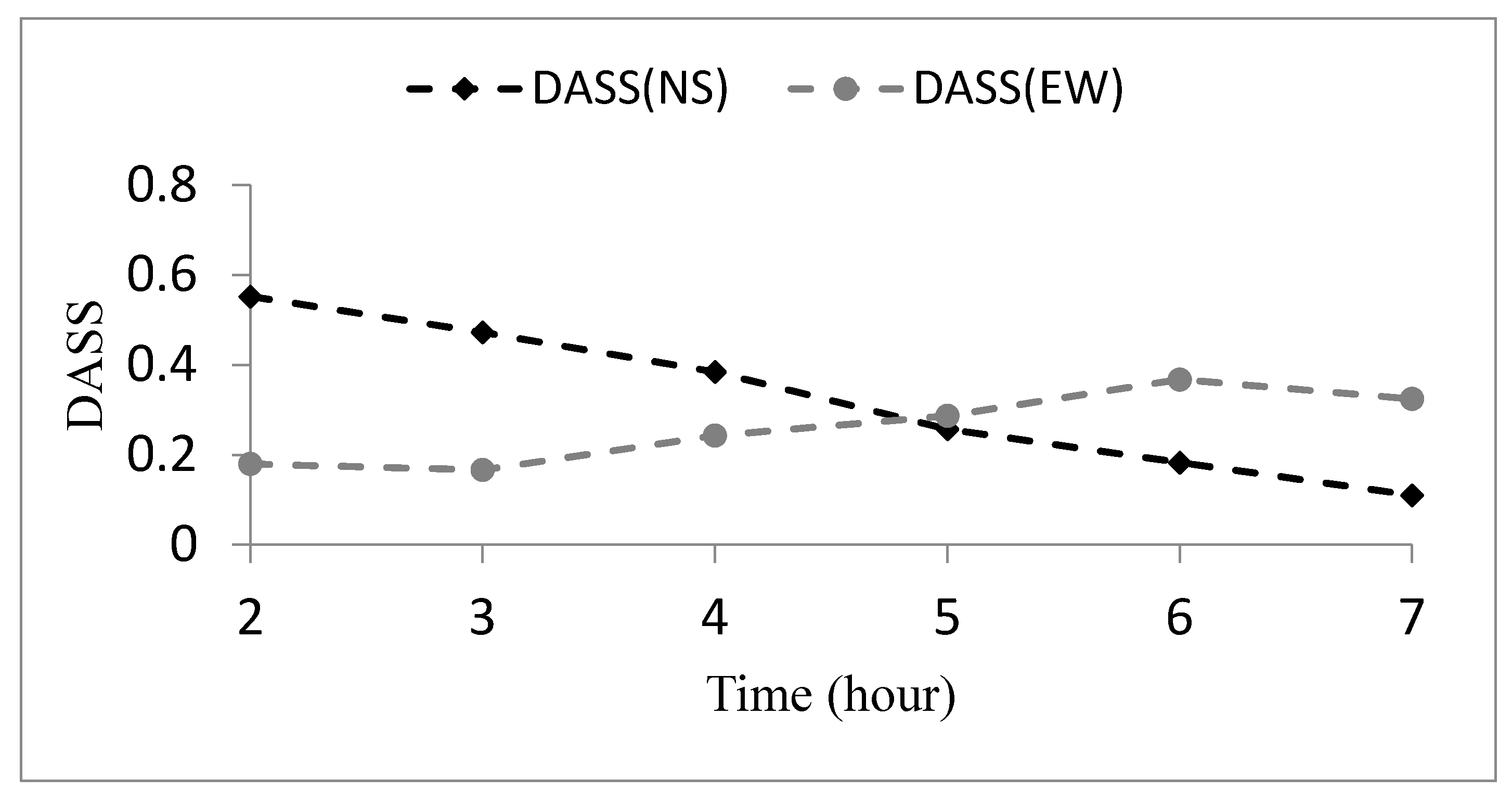
An analogous version of Equation (7) was also used to calculate for surface east–west velocity component. If DASS is greater than zero, then it indicates that the data assimilation model improved the forecasting compared with model NDA0. If DASS is less than zero, then it means the data assimilation contaminated the basic dynamic processes in the model resulting in deterioration in model accuracy. The time series of DASS for both surface current components are shown in Figure 7.
Figure 7 shows that the DASS values for both surface current components were greater than zero over a six-hour forecasting period. This indicated that the application of nudging data assimilation to combine radar data into EFDC model had positive influences on forecasting. During the first three hours (02:00–04:00), values were larger than . This indicated that data assimilation improved the performance of north–south surface velocity component better than east–west surface velocity component. However, during the final three hours (05:00–07:00), improvement of east–west surface velocity component exceed north–south surface velocity component. In general, the range of was larger than that of ; magnitudes of decreased over time, while magnitudes of increased over the first six hours, and then decreased. This was due to that model adaptability in computing east–west surface velocity component after implementing data assimilation procedure was different from that of north–south surface velocity component. A similar trend of skill score to the was obtained when assessing performance of a sea-ice model after implementing data assimilation by Levy, et al. [50]. Moreover, a similar trend of weighted skill score existed in a global weather data assimilation system by Clayton et al. [9]. Averaged in the data assimilation domain during the +6 h forecast was 26%; the averaged was 33%. The analysis indicates that both surface velocity components were significantly improved during the +6 h forecasting when using the nudging data assimilation algorithm to update the model background states at each model computational timestep.
So, although counterintuitive, it is not unusual for DASS to increase with time during certain forecasts. In this case, it is likely that the increase in DASS is due to the relative changes in wind and tidal forcing functions.
4.3. Averaaged Kinetic Energy Assessment
Assessment of model results based on AKE values is a convenient way to determine fundamental correlation between assimilation model results and observations. Breivik and Satra [15], and Xu et al. [51], previously applied AKE to assess model results. The spatially averaged AKE () across the study domain was calculated to assess improvements when using nudging data assimilation. was calculated as follows [15,49,52]:
where is the domain covered by the CODAR system; ds is the integral cell area; is total surface speed.
Water density is assumed constant, and therefore, it is omitted from Equation (8).
The AKE from models and observations was computed in the data assimilation domain at each model forecasting timestep. Hourly data comprised of 48 points from each dataset over a 2-day forecasting period (start from Julian Day 228 02:00) were used for this analysis, which was sufficient to ensure the analysis is meaningful. Time series of AKE values were calculated using Equation (8). Correlation of AKE between model NDA21 and radar data was improved by 12% in comparison with the model NDA0.
4.4. Assessment of Surface Velocity Components
To further compare the improvements among models and radar data in time, time series of surface velocity components at location A (see Figure 1) from six representative nudging data assimilation models are respectively shown in Figure 8 and Figure 9.
Figure 8 and Figure 9 show significant improvements over time of both velocity components appeared in the best data assimilation model NDA21 compared with model NDA0 at point A. Other nudging data assimilation models (NDA10, NDA22–NDA24), with longer data assimilation cycle lengths, had quite a similar trend to model NDA0 during the forecasting period. Although the trend of the north–south velocity component from model NDA21 was different from the radar data (shown in Figure 9), its trend was closer to the radar data than results from the other models. Moreover, the magnitudes of the north–south velocity component were quite small during the analysis period. Because the north–south velocity component was mainly affected by wind forces, using constant wind data in time and space in the model may lead to errors.
4.5. Assessment of Forecasted Surface Flow Fields
Although the above mean surface flow fields showed surface flow patterns during a half-day period, surface flow fields at a representative forecasting time, 03:00 Julian Day 228, are presented in Figure 10, to further illustrate model performance after implementing data assimilation.
The east–west trend of surface currents was stronger in model NDA21 than model NDA0. The general trend in model NDA21 was closer to the radar measured flow field. Improvements of vector direction of surface currents over the data assimilation domain in model NDA21 were 20% compared with model NDA0 at 3:00. This further demonstrated that updating the model background states at each model computational timestep, using nudging assimilation algorithm, significantly enhanced forecasting of surface flows.
5. Discussion
As the difference between observations and model results was weighted using the factor in the nudging data assimilation technique, and then used to update model background states, the complex definition of observation error covariance and model error covariance used in OI and 4D-VAR techniques was not required. Thus, the application of the nudging algorithm is simpler and more efficient than others, such as OI and 4D-VAR data assimilation schemes. This is of great importance for a real-time operational data assimilation forecasting model, which requires timely prediction information for practical operations, such as search and rescue, and oil spill response. Selection of the most appropriate data assimilation algorithm is important when exploring the potential for using HF radar data to improve model performance.
According to a DASS forecast skill score, improvement of velocity component prediction from a nudging data assimilation model updating at each model computational timestep, was more significant than the assimilation model by Ren et al. [13], which indirectly corrected wind stress using HF radar data for the same research domain. Averaged DASS values over six-hour forecasts obtained by Ren et al. [13] were 1% and 23% for east–west and north–south velocity components, respectively; DASS of 26% and 33% were obtained for velocity east–west and north–south components, respectively, in this work, during the same prediction period. Although indirect data assimilation via correcting wind stress using HF radar data significantly improved forecasting of velocity of the north–south component, the influence of data assimilation on velocity of the east–west component was not as good as using a nudging algorithm. This indicated that the approach proposed in this work was more suitable for producing accurate patterns of surface flow fields for the Galway Bay area. Additionally, Gopalakrishnan and Blumberg [5] used a similar nudging data assimilation scheme to combine HF radar data with model background states; improvements of forecasted velocity east–west (or north–south) components in this work were more significant than their assimilation model results based on DASS values. DASS in Galway Bay for velocity east–west (or north–south) component was 26% (33%), in comparison with their values at 18% (7%). This was because the data assimilation cycle length was small, i.e., at each model computational timestep in this work. In short, frequent updating of model background states using a nudging algorithm positively constrains circulation of surface flow fields during the forecasting period, than those assimilation models with longer data assimilation cycle lengths.
The best data assimilation model (NDA21) had a much smaller RMSE value than RMSE values (range 10~20 cm/s) obtained by Zhao et al. [53] using quasi-ensemble Kalman filter with Canadian quick covariance. This may be because hourly radar data were assimilated into models in their work, but a shorter data assimilation cycle length was applied herein. It also showed that application of quasi-ensemble Kalman filter for assimilating radar data was more challenging than using a nudging data assimilation algorithm.
According to the AKE assessment criteria, improvement of AKE over a 2-day forecasting period of 12% in the best nudging data assimilation model in this work, was comparable to the AKE value of 16% over a 2-h forecast obtained by Breivik and Satra [15]. However, at 4-h and 6-h forecasts, correlation of AKE between radar data and assimilation model significantly decreased from 0.58 to 0.38 in Breivik and Satra [15]. Multiple assessment criteria showed that developed nudging data assimilation updating at each model computational timestep using radar data produced comparable, or better results than others. In addition, sensitivity experiments on nudging parameters presented in Table 1 indicated that hindcasting results were more sensitive to the influence depth than the assimilation time scale. Water depths of the assimilation domain covered by CODAR system ranged from ~5–35 m. To examine model performance at spatial locations with different water depths, relationships between depth of influence and the value of are presented in Table 3.
Table 3 shows that the nudging weighing factor, λ, is equal to 1 when water depth is 30 m. Magnitudes of the nudging weighing factor, λ, had the same trend as water depth varies. Significant deviations in Figure 5b existed at some points, due to incorrectly assimilating the increment to model background states using Equation (1). Exploration of the sensitivity of influence depth over a domain needs to be carried out in future research.
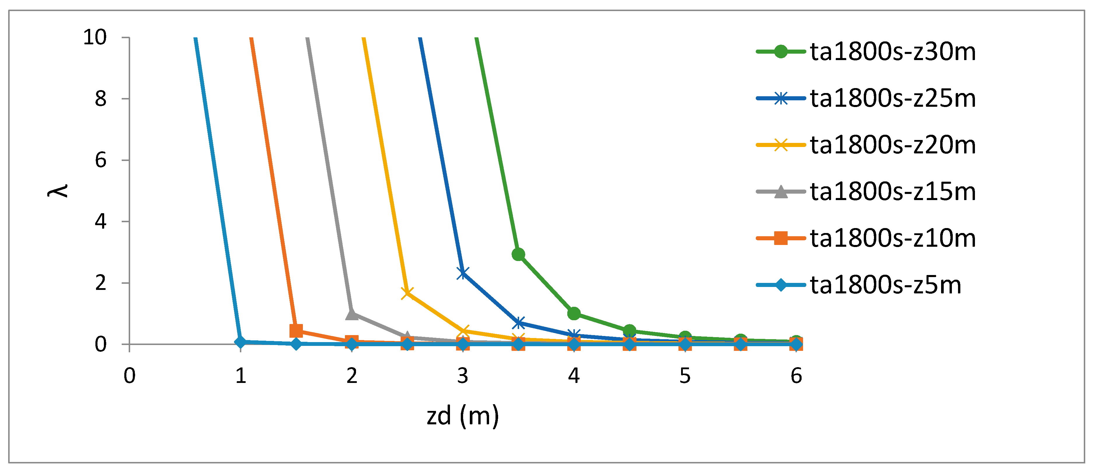
As presented in Table 2, value of the nudging parameter λ, determined by , , and , was different at each model grid. The nudging parameter λ had similar trends relative to and , when was set different values. In order to further investigate relationships among them, an example as is shown in Figure 11. To clearly show the main variation range of λ relative to , and , only parts of plots were shown in Figure 11. The larger the value of z, then the larger λ was, given a fixed value of . It indicated that those points with deeper water depth were nudging to a larger extent. This lead to significant deviation of analysis states from radar data. Use of varying in space can deal with overly nudging at those points, with deeper water depth Moreover, amount of λ, whose value was greater than 10, increased as decreased. It indicated that needed to be large enough, such as 4 m, as in this work. This can ensure that model background states at fewer points were overly nudged than those when was smaller. Thus, presented sensitivity experiments in this work were a must for other cases when using similar nudging data assimilation algorithms.
In addition, models using the same parameters as in model NDA9, NDA11, and NDA12, were performed to assimilate the interpolated radar data at each model computational timestep. On the basis of computation and comparison of RMSE values between assimilation model results and radar data during a 12 h forecasting period, the model using the same nudging parameters as in model NDA9 to assimilate radar data at each model computational timestep overly nudged the analysis states, leading to model instability, and forecasting was significantly larger than radar data. Models using the same nudging parameters as in model NDA11 and NDA12 were developed to assimilate the interpolated radar data at each model computational timestep, respectively. Results from these models were quite similar to outputs from the best model NDA21, but model NDA21 was slightly better than others, in terms of RMSE values between model outputs and radar data during a 12 h forecasting period. Experiments performed in this work indicated that the same nudging parameters can be used to develop nudging data assimilation models with different cycle lengths.
6. Conclusions
Real-time remotely sensing HF radar measurements were blended into a numerical model EFDC using a nudging data assimilation algorithm. The most appropriate nudging parameters were determined based on obtaining minimum RMSE values between modeled results and radar data during a data assimilation period with hourly assimilation. Assimilation of the remotely sensing radar data at each model computational timestep resulted in a good forecasting performance compared with a “free run” model and models with longer data assimilation cycle lengths. The main conclusions from the research are:
- (1)
- Sensitivity tests performed on the nudging data assimilation parameters suggest that an influence depth of 4 m and an assimilation timescale of 1800 s were the suitable values for developing the data assimilation system for Galway Bay based on RMSE analysis during a hindcasting period. Further analysis indicated that surface flow fields were more sensitive to the depth of influence than the assimilation time scale. This is the first study that has investigated the effects of the system parameters on results, and to provide guidance for future application of this algorithm.
- (2)
- The research showed that modelling performance was also quite sensitive to data assimilation cycle lengths. Assimilation of radar data at each model computational timestep significantly improved model forecasting in comparison with using longer data assimilation cycle lengths. The RMSE of the averaged velocity components over a half-day forecasting period between the radar data and the best nudging data assimilation model was smaller than model forecasts using longer cycle lengths. The averaged east–west and north–south velocity components from the best model (NDA21) were improved by 10% and 15%, compared with the “free run”, respectively. However, there were no distinct improvements in RMSE between the other models with longer data assimilation cycle lengths. The results presented herein demonstrated better performance than all other published results in investigating this area. Additionally, results indicated that the same nudging assimilation parameters can be used for models with different cycle lengths.
- (3)
- The calculation of surface flow fields were enhanced during the forecasting period when data assimilation was employed at each model computational timestep. Surface flow fields from other assimilation models with longer cycle lengths did not significantly improve compared with model NDA0. This was the first time such a sensitivity analysis was performed.
- (4)
- The values of DASS generated during this research proved that model NDA21 improved model performance by 26% and 33% for east–west and north–south velocity components, respectively, during a +6 h forecasting period for Galway Bay; these were significant improvements.
- (5)
- Analysis of AKE further proved that updating model background states at each model computational timestep resulted in forecasting improvements. Correlation of AKE between the best nudging data assimilation model NDA21 and the radar data was improved by 12% compared with model NDA0 over a two-day forecasting. The improvement, herein, was comparable with other studies.
- (6)
- Time series graphs at a location within Galway Bay showed that implementation of data assimilation at each model step using interpolated radar data greatly enhanced both surface velocity components during forecasting period, especially for the north–south surface velocity component. Results from other assimilation models with longer data assimilation cycle lengths did not generate distinct improvements on the model forecasts; they followed the same trend as the “free run”.
- (7)
- Surface flow fields at a representative measurement timestep, 03:00 Julian Day 228, show that the best assimilation model produced significantly better surface flow circulation through the domain than the “free run” did. Improvements of vector directions in the domain were in the order of 20% at this time, compared with the “free run”.
In summary, the assimilation of remotely sensed HF radar data using a nudging algorithm is a powerful tool for improving model performance. For the first time, this research presented evidence of the effects of changes in nudging parameters and data assimilation cycle lengths on hydrodynamic forecasting, when applying this algorithm. The nudging algorithm has been shown to be particularly useful when updating is applied at each model computational timestep. Significant improvements in forecasting can last more than six hours after data assimilation; these forecasts can provide useful information for a variety of applications, such as search and rescue and oil spill operations. Sensitivity analysis, as described above, should be carried out for site specific models when using remotely sensed data. In order to explore effects of assimilation with high temporal model updating and to further enhance modelling performance, non-linear interpolated temporal radar data will be conducted in future work.
Acknowledgments
This research was supported by China Scholarship Council (CSC) and National University of Ireland, Galway (NUIG). We would like to thank Informatics Research Unit for Sustainable Engineering (IRUSE) for providing the weather data, Oregon State University (OSU) for providing the OTIS tide software, and Ireland’s High-Performance Computing Centre (ICHEC) for providing computation service.
Author Contributions
Lei Ren and Michael Hartnett conceived and ran models; Lei Ren and Michael Hartnett wrote this paper.
Conflicts of Interest
The authors declare no conflict of interest. The founding sponsors had no role in the design of the study; in the collection, analyses, or interpretation of data; in the writing of the manuscript, and in the decision to publish the results.
References
- Robert, C.L.; Blayo, E.; Verron, J. Comparison of reduced-order, sequential and variational data assimilation methods in the tropical Pacific Ocean. Ocean Dyn. 2006, 56, 624–633. [Google Scholar] [CrossRef]
- Ide, K.; Courtier, P.; Ghil, M.; Lorenc, A.C. Unified notation for data assimilation operational, sequential and variational. J. Meteorol. Soc. Jpn. 1997, 75, 181–189. [Google Scholar] [CrossRef]
- Madsen, H.; Hartnack, J.; Sørensen, J.V.T. Data assimilation in a flood modelling system using the Ensemble Kalman filter. In Proceedings of the XVI International Conference on Computational Methods in Water Resources, Copenhagen, Denmark, 19–22 June 2006. [Google Scholar]
- Evensen, G. The Ensemble Kalman Filter: Theoretical formulation and practical implementation. Ocean Dyn. 2003, 53, 343–367. [Google Scholar] [CrossRef]
- Gopalakrishnan, G.; Blumberg, A.F. Assimilation of HF radar-derived surface currents on tidal-timescales. J. Oper. Oceanogr. 2012, 5, 75–87. [Google Scholar] [CrossRef]
- Isern-Fontanet, J.; Ballabrera-Poy, J.; Turiel, A.; Garcia-Ladona, E. Retrieval and assimilation of velocities at the ocean surface. Nonlinear Process. Geophys. 2017, 1–37. [Google Scholar] [CrossRef]
- Moore, A.M.; Arango, H.G.; Broquet, G.; Powell, B.S.; Weaver, A.T.; Zavala-Garay, J. The Regional Ocean Modeling System (ROMS) 4-dimensional variational data assimilation systems: Part I—System overview and formulation. Prog. Oceanogr. 2011, 91, 34–49. [Google Scholar] [CrossRef]
- Hoteit, I.; Cornuelle, B.; Kim, S.Y.; Forget, G.; Köhl, A.; Terrill, E. Assessing 4D-VAR for dynamical mapping of coastal high-frequency radar in San Diego. Dyn. Atmos. Oceans 2009, 48, 175–197. [Google Scholar] [CrossRef]
- Clayton, A.M.; Lorenc, A.C.; Barker, D.M. Operational implementation of a hybrid ensemble/4D-Var global data assimilation system at the Met Office. Q. J. R. Meteorol. Soc. 2013, 139, 1445–1461. [Google Scholar] [CrossRef]
- Ngodock, H.; Carrier, M. A 4DVAR system for the Navy Coastal Ocean Model. Part I: System description and assimilation of synthetic observations in Monterey Bay. Mon. Weather Rev. 2014, 142, 2085–2107. [Google Scholar] [CrossRef]
- Powell, B.S.; Arango, H.G.; Moore, A.M.; Di Lorenzo, E.; Milliff, R.F.; Foley, D. 4DVAR data assimilation in the Intra-Americas Sea with the Regional Ocean Modeling System (ROMS). Ocean Model. 2008, 25, 173–188. [Google Scholar] [CrossRef]
- Paduan, J.D.; Shulman, I. HF radar data assimilation in the Monterey Bay area. J. Geophys. Res. 2004, 109, 434–446. [Google Scholar] [CrossRef]
- Ren, L.; Nash, S.; Hartnett, M. Forecasting of surface currents via correcting wind stress with assimilation of high-frequency radar data in a three-dimensional model. Adv. Meteorol. 2016, 2016, 1–12. [Google Scholar] [CrossRef]
- Barth, A.; Alvera-Azcarate, A.; Weisberg, R.H. Assimilation of high-frequency radar currents in a nested model of the West Florida Shelf. J. Geophys. Res. 2008, 113, 1–15. [Google Scholar] [CrossRef]
- Breivik, O.; Satra, O. Real time assimilation of HF radar currents into a coastal ocean model. J. Mar. Syst. 2001, 28, 161–182. [Google Scholar] [CrossRef]
- Fan, S.; Oey, L.Y.; Hamilton, P. Assimilation of drifter and satellite data in a model of the Northeastern Gulf of Mexico. Cont. Shelf Res. 2004, 24, 1001–1013. [Google Scholar] [CrossRef]
- Castellari, S.; Griffa, A.; Ozgokmen, T.M.; Poulain, P.M. Prediction of particle trajectories in the Adriatic sea using Lagrangian data assimilation. J. Mar. Syst. 2001, 29, 33–50. [Google Scholar] [CrossRef]
- Lin, X.H.; Oey, L.Y.; Wang, D.P. Altimetry and drifter data assimilations of loop current and eddies. J. Geophys. Res. 2007, 112. [Google Scholar] [CrossRef]
- Dabrowski, T. A Flushing Study Analysis of Selected Irish Waterbodies. Ph.D. Thesis, National University of Ireland Galway, Galway, Ireland, 2005. [Google Scholar]
- O’Donncha, F.; Hartnett, M.; Nash, S.; Ren, L.; Ragnoli, E. Characterizing observed circulation patterns within a bay using HF radar and numerical model simulations. J. Mar. Syst. 2014, 142, 96–110. [Google Scholar] [CrossRef]
- Wang, J.; Dizaji, R.; Ponsford, A.M. Analysis of clutter distribution in bistatic high frequency surface wave radar. In Proceedings of the 2004 Canadian Conference on Electrical and Computer Engineering, Niagara Falls, ON, Canada, 2–5 May 2004; pp. 1301–1304. [Google Scholar]
- Haus, B.K.; Wang, J.D.; Rivera, J.; Martinez-Pedraja, J.; Smith, N. Remote radar measurement of shelf currents off key largo, Florida, U.S.A. Estuar. Coast. Shelf Sci. 2000, 51, 553–569. [Google Scholar] [CrossRef]
- Ojo, T.O.; Bonner, J.S.; Page, C.A. Simulation of constituent transport using a reduced 3D constituent transport model (CTM) driven by HF Radar: Model application and error analysis. Environ. Model. Softw. 2007, 22, 488–501. [Google Scholar] [CrossRef]
- Lipa, B.; Barrick, D.; Alonso-Martirena, A.; Fernandes, M.; Ferrer, M.; Nyden, B. Brahan project high frequency radar ocean measurements: Currents, winds, waves and their interactions. Remote Sens. 2014, 6, 12094–12117. [Google Scholar] [CrossRef]
- Lipa, B.; Whelan, C.; Rector, B.; Nyden, B. HF radar bistatic measurement of surface current velocities: drifter comparisons and radar consistency checks. Remote Sens. 2009, 1, 1190–1211. [Google Scholar] [CrossRef]
- Shulman, I.; Paduan, J.D. Assimilation of HF radar-derived radials and total currents in the Monterey Bay area. Deep Sea Res. Part II Top. Stud. Oceanogr. 2009, 56, 149–160. [Google Scholar] [CrossRef] [Green Version]
- Paduan, J.D.; Washburn, L. High-frequency radar observations of ocean surface currents. Ann. Rev. Mar. Sci. 2013, 5, 115–136. [Google Scholar] [CrossRef] [PubMed]
- Emery, B.M.; Washburn, L.; Harlan, J.A. Evaluating radial current measurements from CODAR high-frequency radars with moored current meters. J. Atmos. Ocean. Technol. 2003, 21, 1259–1271. [Google Scholar] [CrossRef]
- Liu, Y.; Weisberg, R.H.; Merz, C.R.; Lichtenwalner, S.; Kirkpatrick, G.J. HF Radar performance in a low-energy environment: CODAR SeaSonde experience on the West Florida Shelf. J. Atmos. Ocean. Technol. 2010, 27, 1689–1710. [Google Scholar] [CrossRef]
- Hamrick, J.M. EFDC Technical Memorandum; US Environmental Protection: Fairfax, VA, USA, 2006.
- TetraTech. The Environmental Fluid Dynamics Code Theory and Computation Volume 1: Hydrodynamics and Mass Transport; Tetra Tech, Inc.: Virginia Beach, VA, USA, 2007; p. 60. [Google Scholar]
- Hamrick, J.M. A Three-Dimensional Environmental Fluid Dynamics Computer Code: Therotical and Computatonal Aspects; Virginia Institute of Marine Science: Gloucester Point, VA, USA, 1992. [Google Scholar]
- Zou, R.; Carter, S.; Shoemaker, L.; Parker, A.; Henry, T. An integrated hydrodynamic and water quality modeling system to support nutrient TMDL development for Wissahickon Creek. J. Environ. Eng. 2006, 132, 555–566. [Google Scholar] [CrossRef]
- Jin, K.R.; Ji, Z.G. Case Study: Modeling of sediment transport and wind-wave impact in Lake Okeechobee. J. Hydraul. Eng. 2004, 130, 1055–1067. [Google Scholar] [CrossRef]
- O’Donncha, F.; Hartnett, M.; Nash, S. Physical and numerical investigation of the hydrodynamic implications of aquaculture farms. Aquac. Eng. 2013, 52, 14–26. [Google Scholar] [CrossRef]
- Wen, L. Three-Dimensional Hydrodynamic Modelling in Galway Bay; University College Galway: Galway, Ireland, 1995. [Google Scholar]
- Nagle, D. Modelling and Observation of Wind-Driven Circulation in Galway Bay; National University of Ireland Galway: Galway, Ireland, 2013. [Google Scholar]
- Ren, L.; Nash, S.; Hartnett, M. Observation and modeling of tide- and wind-induced surface currents at Galway Bay. Water Sci. Eng. 2015, 8, 345–352. [Google Scholar] [CrossRef]
- Egbert, G.D.; Erofeeva, S.Y. Efficient inverse modeling of barotropic ocean tides. J. Atmos. Ocean. Technol. 2002, 19, 183. [Google Scholar] [CrossRef]
- Padman, L. A barotropic inverse tidal model for the Arctic Ocean. Geophys. Res. Lett. 2004, 31, 1–4. [Google Scholar] [CrossRef]
- Gopalakrishnan, G. Surface Current Observations Using High Frequency Radar and Its Assimilation into the New York Harbor Observing and Prediction System. Ph.D. Thesis, Stevens Institute of Technology, Hoboken, NJ, USA, 2008. [Google Scholar]
- Houser, P.R.; Shuttleworth, W.J.; Famiglietti, J.S.; Gupta, H.V.; Syed, K.H.; Goodrich, D.C. Integration of soil moisture remote sensing and hydrologic modeling using data assimilation. Water Resour. Res. 1998, 34, 3405–3420. [Google Scholar] [CrossRef]
- Rusu, L.; Guedes Soares, C. Impact of assimilating altimeter data on wave predictions in the western Iberian coast. Ocean Model. 2015, 96, 126–135. [Google Scholar] [CrossRef]
- Stauffer, D.R.; Seaman, N.L. Use of four-dimensional data assimilation in a limited-area mesoscale model. Part I: Experiments with synoptic-scale data. Mon. Weather Rev. 1990, 118, 1250–1277. [Google Scholar] [CrossRef]
- Sun, J. Convective-scale assimilation of radar data: Progress and challenges. Q. J. R. Meteorol. Soc. 2005, 131, 3439–3463. [Google Scholar] [CrossRef]
- Agostinho, P.; Gil, A.; Galeano, J.C. N.U.I Galway CODAR SeaSonde HF Radar System; Qualitas Remos: Galway, Ireland, 2012. [Google Scholar]
- Ren, L.; Nash, S.; Hartnett, M. Renewable energies offshore. In Chapter 24 Data Assimilation with High-Frequency (HF) Radar Surface Currents at a Marine Renewable Energy Test Site; Soares, C.G., Ed.; CRC Press: London, UK, 2015. [Google Scholar]
- Toba, Y. Local balance in the air-sea boundary processes. J. Oceanogr. Soc. Jpn. 1973, 29, 209–220. [Google Scholar] [CrossRef]
- Ren, L.; Hartnett, M.; Nash, S. Assessment methods of data assimilation in oceanographic model forecasting. In Proceedings of the 36th IAHR World Congress, Delft, The Netherlands, 28 June–3 July 2015; pp. 1–10. [Google Scholar]
- Levy, G.; Coon, M.; Nguyen, G.; Sulsky, D. Physically-based data assimilation. Geosci. Model Dev. 2010, 3, 669–677. [Google Scholar] [CrossRef] [Green Version]
- Xu, J.; Huang, J.; Gao, S.; Cao, Y. Assimilation of high frequency radar data into a shelf sea circulation model. J. Ocean Univ. China 2014, 13, 572–578. [Google Scholar] [CrossRef]
- Thiebaux, H.J. Anisotropic correction functions for objective analysis. Mon. Weather Rev. 1976, 104, 994–1002. [Google Scholar] [CrossRef]
- Zhao, J.; Chen, X.; Xu, J.; Hu, W.; Chen, J.; Pohlmann, T. Assimilation of surface currents into a regional model over Qingdao coastal waters of China. Acta Oceanol. Sin. 2013, 32, 21–28. [Google Scholar] [CrossRef]
Figure 1.
Deployment of HF radar system in Galway Bay (C1 indicates the HF radar on Mutton Island; C2 indicates the HF radar located near Spiddal; A indicates a reference point for analysis).
Figure 1.
Deployment of HF radar system in Galway Bay (C1 indicates the HF radar on Mutton Island; C2 indicates the HF radar located near Spiddal; A indicates a reference point for analysis).
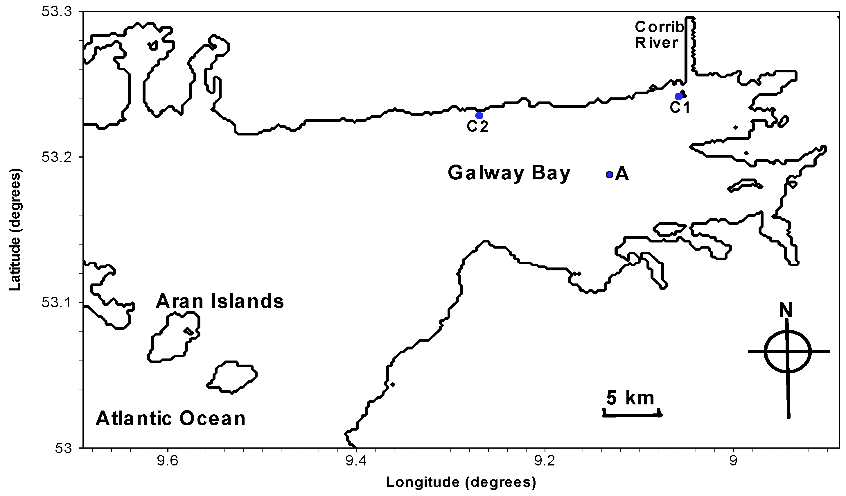
Figure 2.
Flowchart of EFDC model (shaded boxes indicate the calculation process for the hydrodynamic variables of interest for data assimilation).
Figure 2.
Flowchart of EFDC model (shaded boxes indicate the calculation process for the hydrodynamic variables of interest for data assimilation).

Figure 3.
Flowchart of data assimilation in main program HDMT.FOR of EFDC (shaded part indicates new subroutine for data assimilation).
Figure 3.
Flowchart of data assimilation in main program HDMT.FOR of EFDC (shaded part indicates new subroutine for data assimilation).
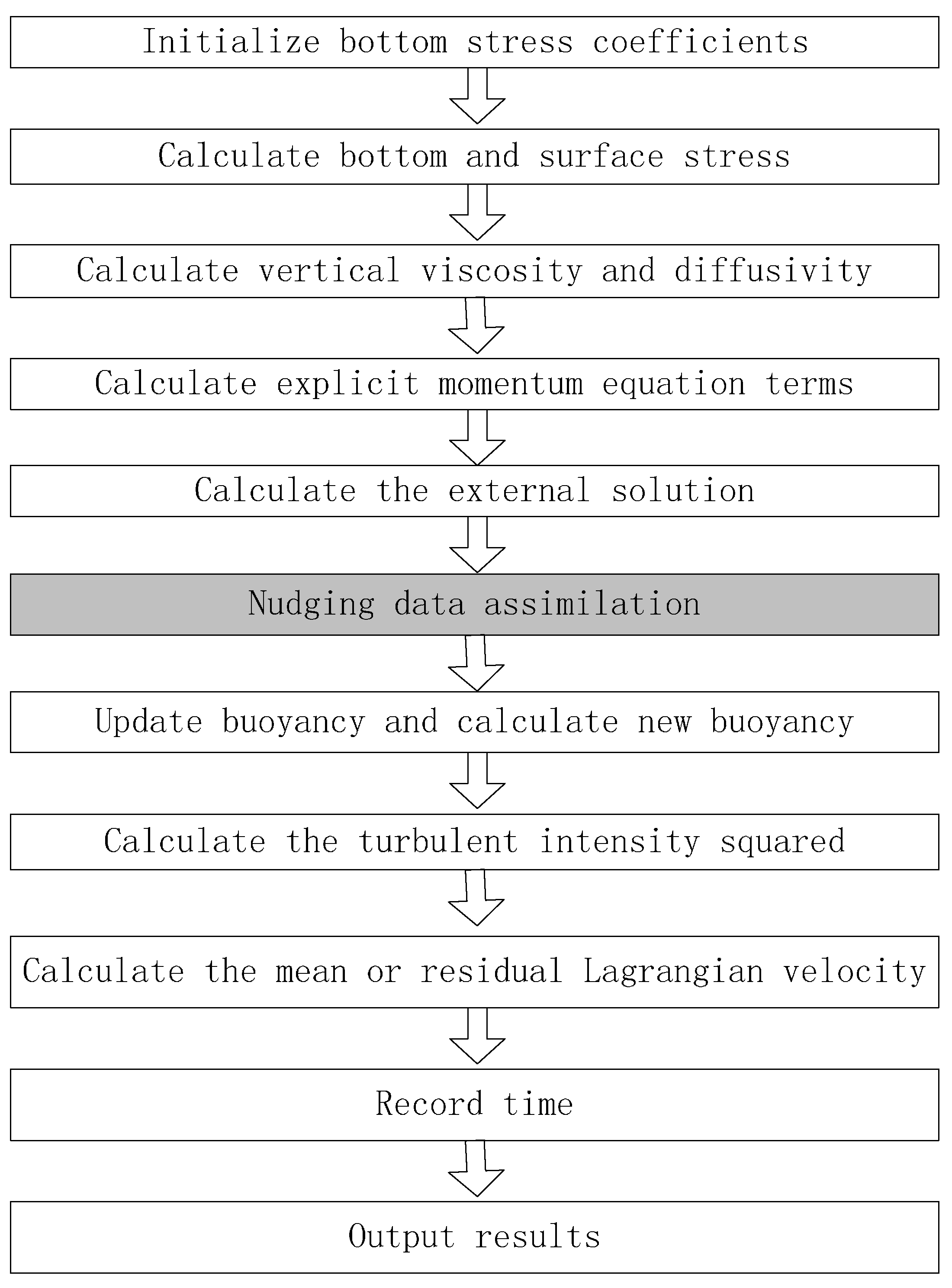
Figure 4.
Flow chart of implementing a nudging algorithm in EFDC model.
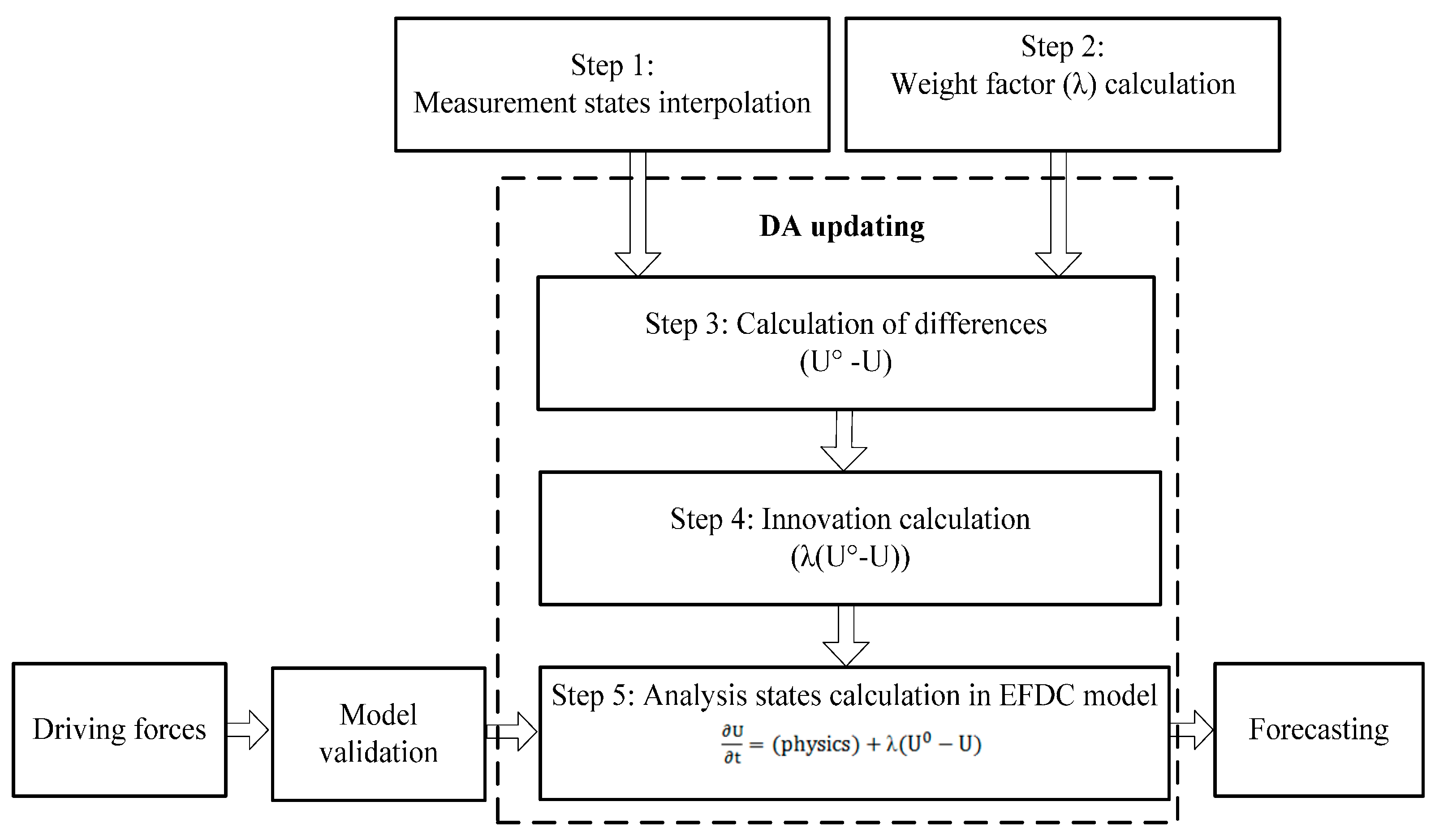
Figure 5.
Mean surface flow fields during Julian Day 220–228 01:00 ((a) is averaged flow field from model NDA0, (b–e) are averaged flow fields from model NDA9-NDA12, respectively; (f) is averaged flow field of radar data).
Figure 5.
Mean surface flow fields during Julian Day 220–228 01:00 ((a) is averaged flow field from model NDA0, (b–e) are averaged flow fields from model NDA9-NDA12, respectively; (f) is averaged flow field of radar data).
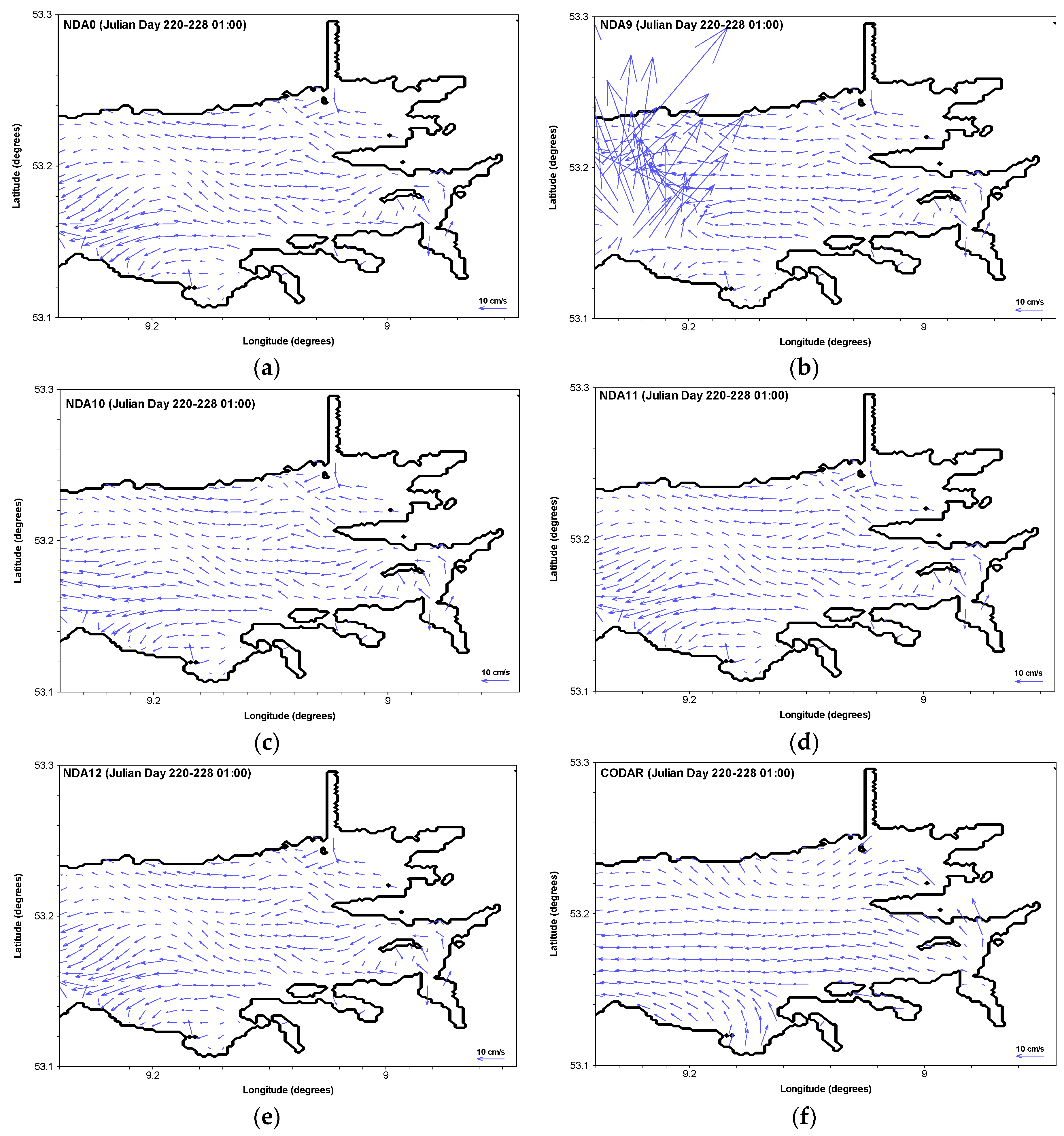
Figure 6.
Mean surface flow fields ((a) results from model NDA0; (b–e) results from model NDA21-NDA24, respectively; (f) results from model NDA10; (g) radar data).
Figure 6.
Mean surface flow fields ((a) results from model NDA0; (b–e) results from model NDA21-NDA24, respectively; (f) results from model NDA10; (g) radar data).
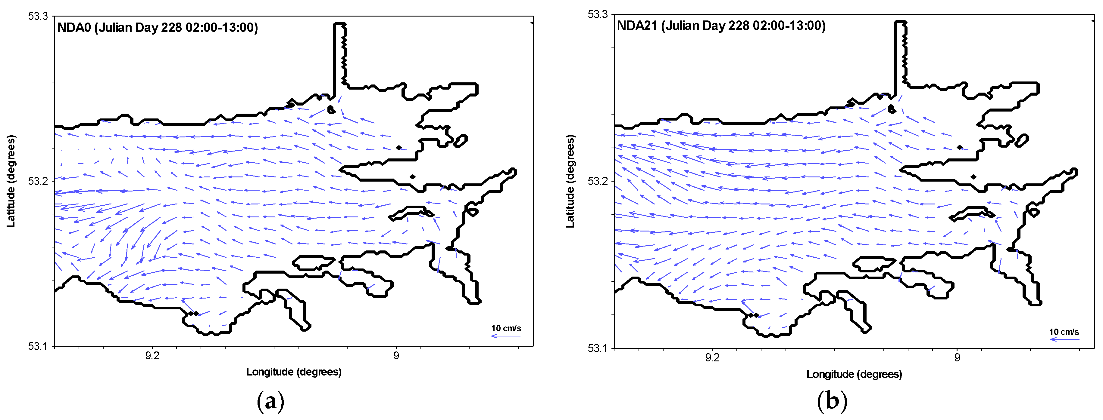
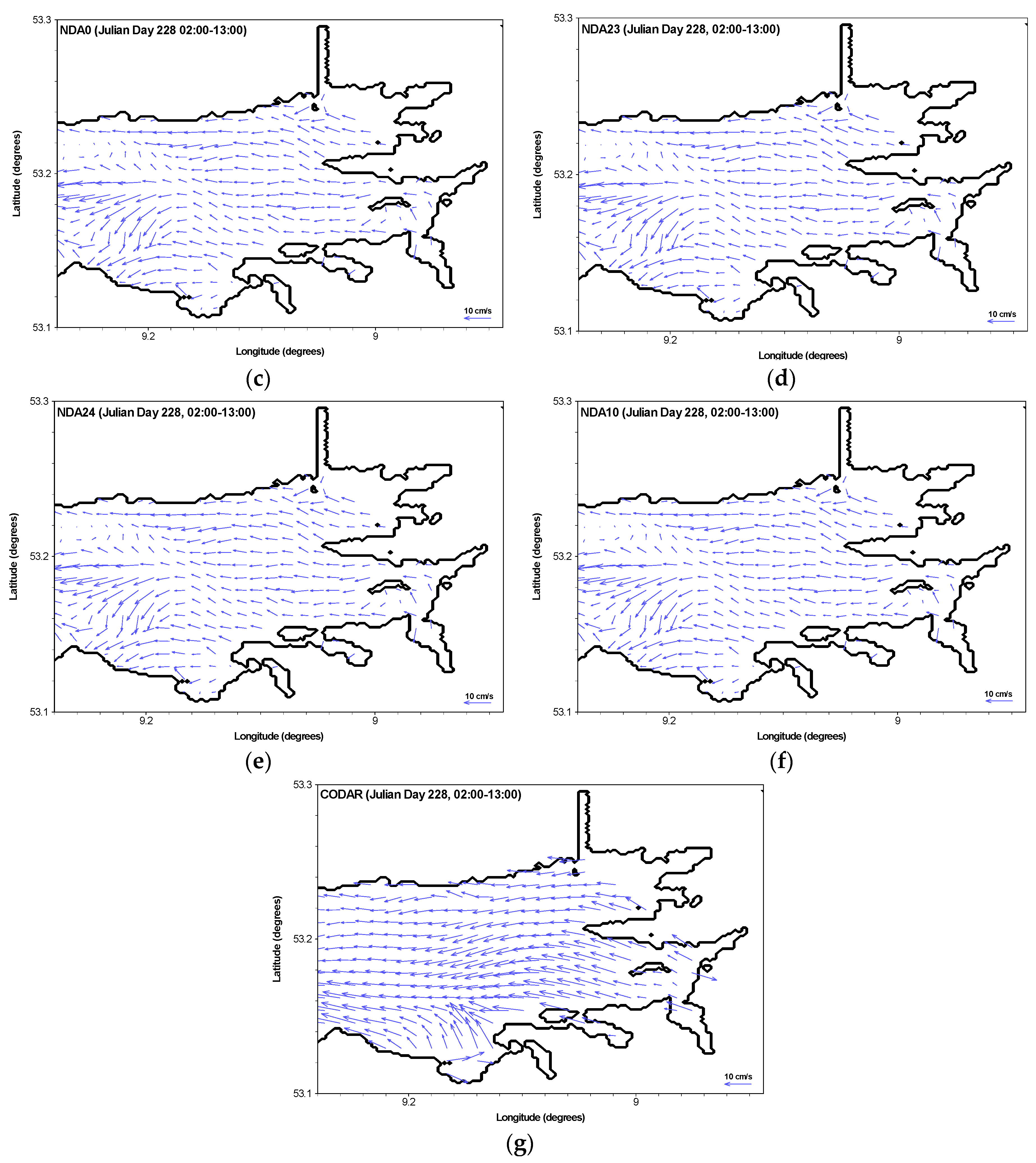
Figure 7.
DASS of model NDA21 during 02:00–07:00 Julian Day 228.

Figure 8.
Time series of east–west velocity component.
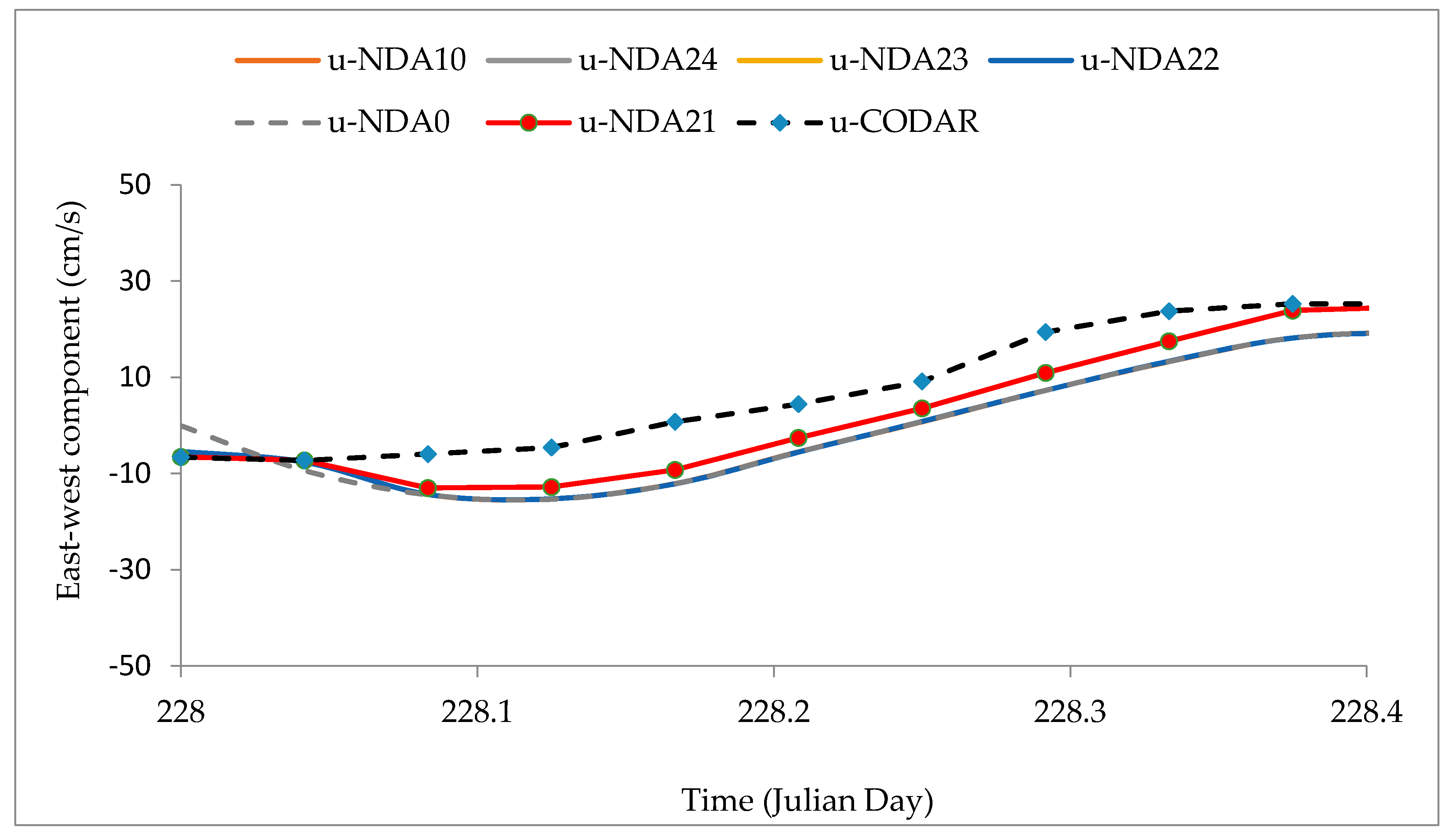
Figure 9.
Time series of north–south velocity component.
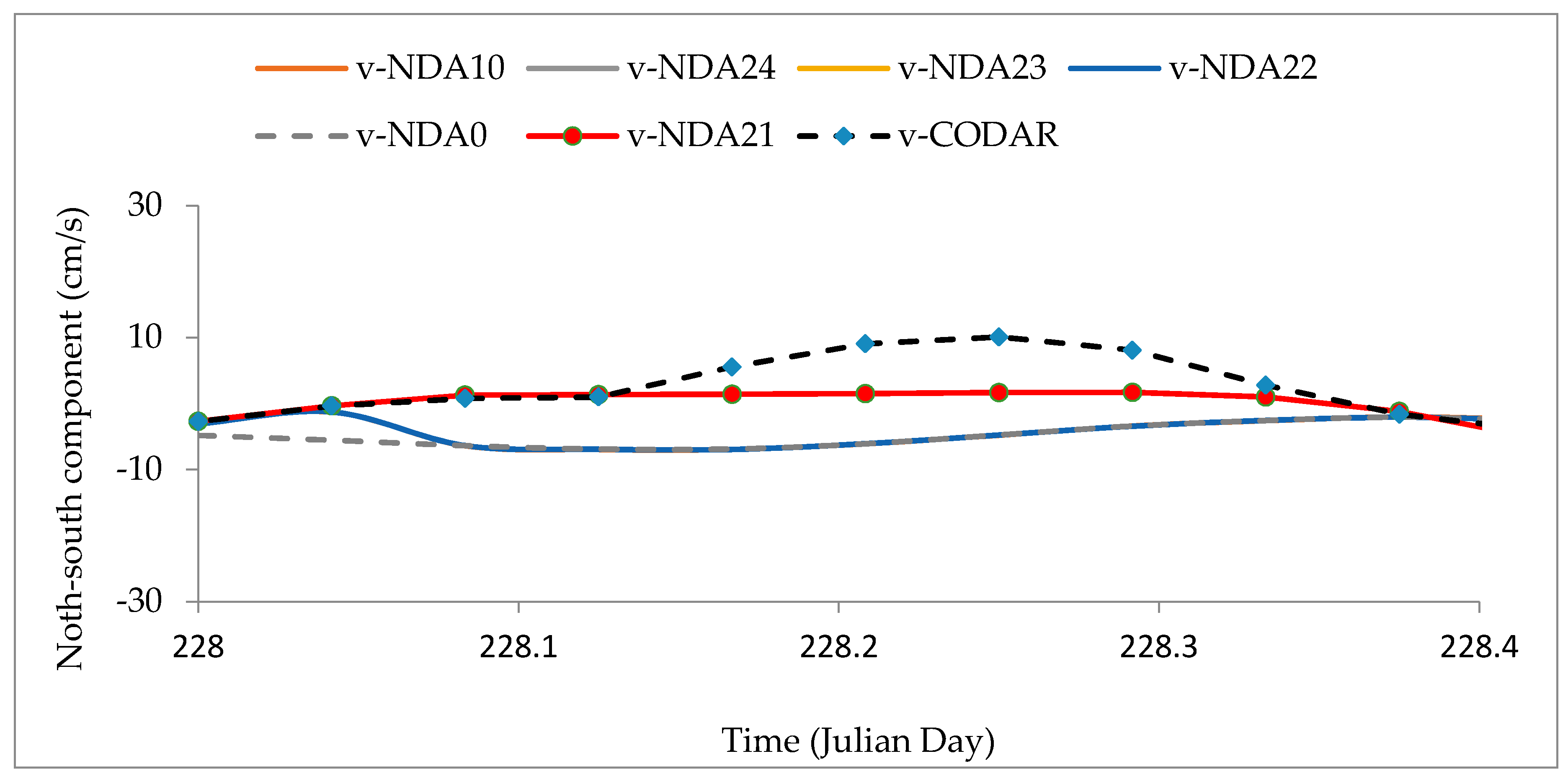
Figure 10.
Surface flow fields at 03:00 Julian Day 228 ((a) forecast from the model NDA0; (b) radar data; (c) forecast from the model NDA21).
Figure 10.
Surface flow fields at 03:00 Julian Day 228 ((a) forecast from the model NDA0; (b) radar data; (c) forecast from the model NDA21).
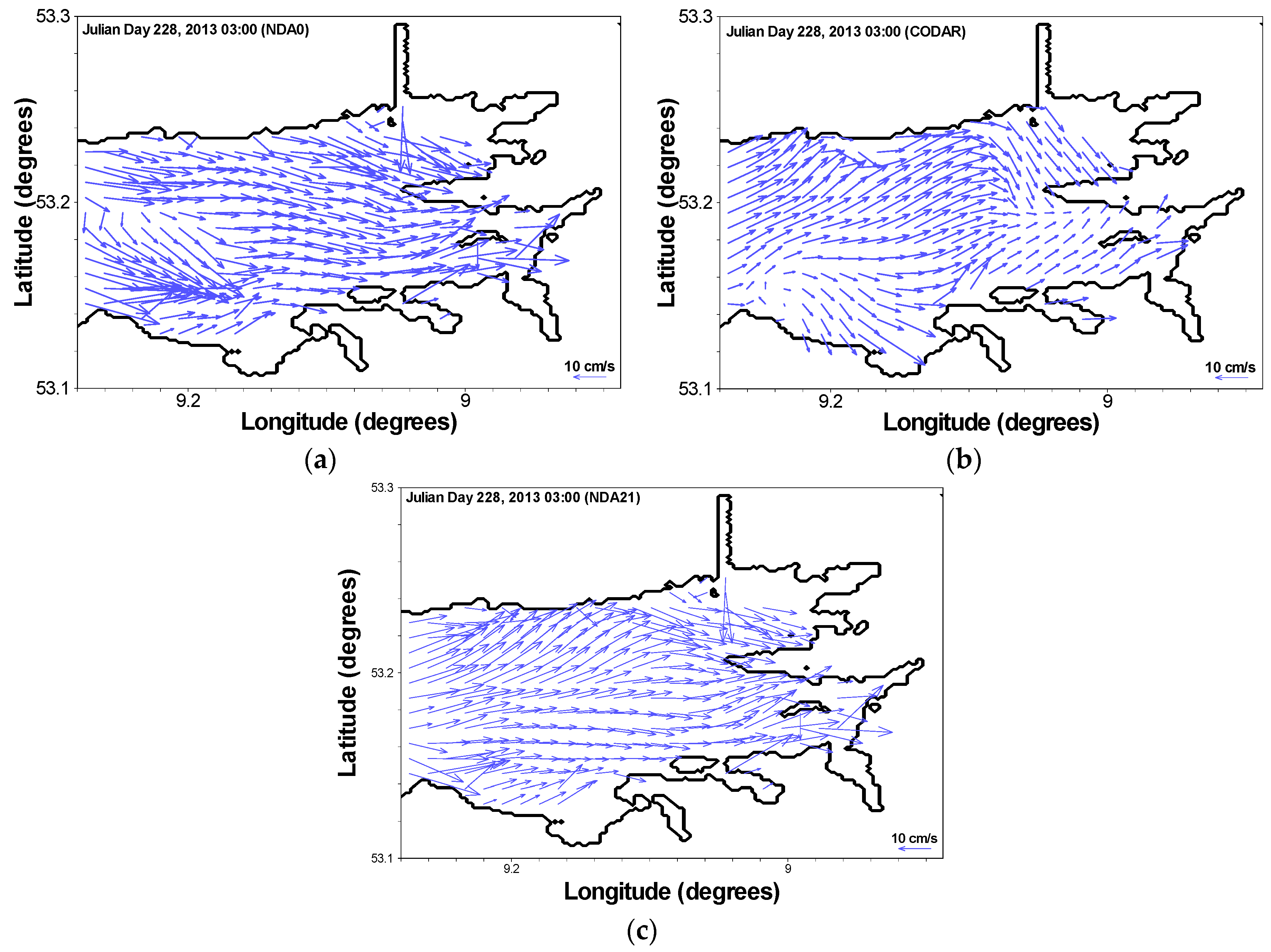
Figure 11.
Relationship among nudging parameters.


Table 1.
Nudging Data Assimilation Test Models.
| Model | Zd (m) | Ta (s) | RMSE (u, cm/s) | RMSE (v, cm/s) | RMSE (u, v, cm/s) |
|---|---|---|---|---|---|
| NDA0 | - | - | 8.71 | 7.70 | 11.62 |
| NDA1 | 3 | 1200 | 79.61 | 67.79 | 104.56 |
| NDA2 | 4 | 1200 | 8.13 | 7.13 | 10.81 |
| NDA3 | 5 | 1200 | 8.11 | 7.15 | 10.81 |
| NDA4 | 6 | 1200 | 8.44 | 7.45 | 11.26 |
| NDA5 | 3 | 1500 | 63.26 | 53.93 | 83.13 |
| NDA6 | 4 | 1500 | 7.88 | 6.92 | 10.48 |
| NDA7 | 5 | 1500 | 8.22 | 7.25 | 10.96 |
| NDA8 | 6 | 1500 | 8.50 | 7.50 | 11.33 |
| NDA9 | 3 | 1800 | 52.43 | 44.69 | 68.89 |
| NDA10 | 4 | 1800 | 7.80 | 6.86 | 10.39 |
| NDA11 | 5 | 1800 | 8.29 | 7.31 | 11.06 |
| NDA12 | 6 | 1800 | 8.53 | 7.53 | 11.38 |
| NDA13 | 3 | 2100 | 44.71 | 38.14 | 58.77 |
| NDA14 | 4 | 2100 | 7.81 | 6.86 | 10.40 |
| NDA15 | 5 | 2100 | 8.35 | 7.37 | 11.14 |
| NDA16 | 6 | 2100 | 8.55 | 7.56 | 11.41 |
| NDA17 | 3 | 2400 | 38.97 | 33.26 | 51.24 |
| NDA18 | 4 | 2400 | 7.84 | 6.90 | 10.44 |
| NDA19 | 5 | 2400 | 9.39 | 7.40 | 11.96 |
| NDA20 | 6 | 2400 | 8.57 | 7.57 | 11.43 |
indicates depth of influence; is assimilation scale.
Table 2.
Nudging Cycle Length Test Models (+12 h forecasting).
| Model | NDA0 | NDA21 | DA22 | NDA23 | NDA24 | NDA10 |
|---|---|---|---|---|---|---|
| Cycle Length (minutes) | - | MS * | 1 | 5 | 15 | 60 |
| RMSE (u, cm/s) | 8.2131 | 7.3618 | 8.2189 | 8.2087 | 8.2138 | 8.2054 |
| RMSE (v, cm/s) | 6.0902 | 5.2062 | 6.1026 | 6.093 | 6.0938 | 6.0956 |
| RMSE (u, v, cm/s) | 10.2247 | 9.0167 | 10.2368 | 10.2229 | 10.2275 | 10.2218 |
* Note that MS indicates assimilation was performed at each model computational timestep.
Table 3.
Relationship between z and λ (zd = 4 m, ta = 1800 s).
| Z (m) | (z/zd) | Exp (z/zd) | λ |
|---|---|---|---|
| 5 | 1.25 | 3.49 | 0.00 |
| 15 | 3.75 | 42.52 | 0.02 |
| 20 | 5.00 | 148.41 | 0.08 |
| 25 | 6.25 | 518.01 | 0.29 |
| 30 | 7.50 | 1808.04 | 1.00 |
| 35 | 8.75 | 6310.69 | 3.51 |
© 2017 by the authors. Licensee MDPI, Basel, Switzerland. This article is an open access article distributed under the terms and conditions of the Creative Commons Attribution (CC BY) license (http://creativecommons.org/licenses/by/4.0/).
Share and Cite
MDPI and ACS Style
Ren, L.; Hartnett, M. Hindcasting and Forecasting of Surface Flow Fields through Assimilating High Frequency Remotely Sensing Radar Data. Remote Sens. 2017, 9, 932. https://doi.org/10.3390/rs9090932
AMA Style
Ren L, Hartnett M. Hindcasting and Forecasting of Surface Flow Fields through Assimilating High Frequency Remotely Sensing Radar Data. Remote Sensing. 2017; 9(9):932. https://doi.org/10.3390/rs9090932
Chicago/Turabian StyleRen, Lei, and Michael Hartnett. 2017. "Hindcasting and Forecasting of Surface Flow Fields through Assimilating High Frequency Remotely Sensing Radar Data" Remote Sensing 9, no. 9: 932. https://doi.org/10.3390/rs9090932
Note that from the first issue of 2016, this journal uses article numbers instead of page numbers. See further details here.