
A Convolutional Neural Network-Based 3D Semantic Labeling Method for ALS Point Clouds


State Key Laboratory of Information Engineering in Surveying, Mapping and Remote Sensing, Wuhan University, Wuhan 430000, Hubei, China
*
Author to whom correspondence should be addressed.
Remote Sens. 2017, 9(9), 936; https://doi.org/10.3390/rs9090936
Submission received: 1 August 2017
/
Revised: 23 August 2017
/
Accepted: 8 September 2017
/
Published: 10 September 2017
(This article belongs to the Special Issue Remote Sensing for 3D Urban Morphology)
Abstract
:3D semantic labeling is a fundamental task in airborne laser scanning (ALS) point clouds processing. The complexity of observed scenes and the irregularity of point distributions make this task quite challenging. Existing methods rely on a large number of features for the LiDAR points and the interaction of neighboring points, but cannot exploit the potential of them. In this paper, a convolutional neural network (CNN) based method that extracts the high-level representation of features is used. A point-based feature image-generation method is proposed that transforms the 3D neighborhood features of a point into a 2D image. First, for each point in the ALS data, the local geometric features, global geometric features and full-waveform features of its neighboring points within a window are extracted and transformed into an image. Then, the feature images are treated as the input of a CNN model for a 3D semantic labeling task. Finally, to allow performance comparisons with existing approaches, we evaluate our framework on the publicly available datasets provided by the International Society for Photogrammetry and Remote Sensing Working Groups II/4 (ISPRS WG II/4) benchmark tests on 3D labeling. The experiment results achieve 82.3% overall accuracy, which is the best among all considered methods.
1. Introduction
The classification of 3D point clouds has generated great attention in the fields of computer vision, remote sensing, and photogrammetry. In recent decades, airborne laser scanning (ALS) has become important in acquiring 3D point clouds. The ALS point clouds allow an automated analysis of large areas in terms of assigning a (semantic) class label to each point of the considered 3D point cloud. Researchers have mainly focused on using supervised statistical methods to classify the data because these methods are more flexible for handling variations in the appearance of objects compared to model-based approaches. In addition to generative classifiers to model the joint distribution of the data and labels [1], modern discriminative methods such as Adaboost [2], Support Vector Machine (SVM) [3] and Random Forest (RF) [4,5] are used. For example, Chehata [6] applied the RF to classify full-waveform LiDAR data. Various multi-echo and full-waveform LiDAR features can be processed and Random Forests are used since they provide an accurate classification and run efficiently on large datasets. Mallet [7] used a point-based multi-class SVM for urban area LiDAR data classification. A support vector machine classifier was used to label the point cloud according to various scenarios based on the rank of the features. He also used the SVM [8] to study the potential of full-waveform data through the automatic classification of urban areas in building, ground, and vegetation points. Weinmann [9] used 10 different supervised classifiers accompanied by 7 neighborhood definitions, 21 geometric features and 7 approaches for feature selection to classify the 3D scene. The end-users would not only observe the performance of single classifiers but also see a comprehensive comparison. However, both methods classify each point independently without considering the labels of its neighborhood.
Thus, spatial regularization tools are added into the classification period. Spatial dependencies between the object classes can be trained to improve the results using methods such as Markov random fields (MRF) [10] and conditional random fields (CRF) [11]. Anguelov [12] used a subclass of the MRF to classify a terrestrial point cloud into four object classes. The MRF models incorporate a large set of diverse features and enforce the preference that neighboring points have the same classification label. Shapovalov [13] used non-associative Markov networks for the point cloud classification and showed how to perform a tractable MAP inference in a network with non-attractive pairwise potentials to obtain better results. By defining classes of 3D geometric surfaces and making use of the CRF, Rusu [14] classified the 3D point clouds. Niemeyer [15] used the CRF for urban scene classification with full waveform LiDAR data. A Random Forest classifier was integrated into a CRF framework, showing that considering the context and using a large number of features is beneficial.
Although the existing methods have performed well in ALS point clouds classification, further development is still needed to increase the potential of point-based features. We want to utilize fully the limited features that are extracted from neighboring points around the labeled point, and apply these features to train a deep neural network that will be used for the future use of unlabeled point clouds. Deep convolutional neural networks (CNNs) [16,17,18,19] play an important role in deep learning theory for their ability to extract high-level representations through compositions of low-level features [20]. Boulch [21] applied CNNs to point cloud labeling. He picked several suitable snapshots of the point cloud, generated the red–green–blue and geometric composite images, and then performed a pixel-wise labeling of each pair of 2D snapshots using convolutional neural networks. Finally, a fast back-projection of the label predictions was performed in 3D space to label every point. This method obtained the best results on the semantic-8 [22] dataset. The points were scanned statically with state-of-the-art equipment and contain very fine details, giving a point density that is much higher than most of the ALS point clouds. An appropriate way that was proposed for handling this was when Hu [23] used the CNN to generate the digital terrain model (DTM) for the ALS point clouds. A point-to-image framework was built such that for every point with spatial context, the neighboring points within a window are extracted and transformed into an image. Then, the classification of a point can be treated as the classification of an image. Using these images to train a CNN model, this method achieved a satisfactory performance in the DTM-generation task, which is a binary classification problem. However, there are still some problems in Hu’s method when facing additional object classes of interest.
In the present study, we improve Hu’s method in the image-generation procedure. We obtain training samples from the labeled ALS point clouds. Unlike Hu’s method, we propose a single point-based method to generate the feature image. For each point in the ALS data, the image is generated from its neighboring points using their local geometric features, global geometric features and full-waveform features. Then, we train the CNN model using the labeled data and use the model for the final semantic labeling task.
2. Methodology
The workflow of our method is shown in Figure 1. First, we transfer the classification of a point to the classification of its corresponding feature image. Then, we train a CNN model with the feature images of the labeled points. Finally, we use the trained model to classify the unlabeled data.
2.1. Convolutional Neural Network
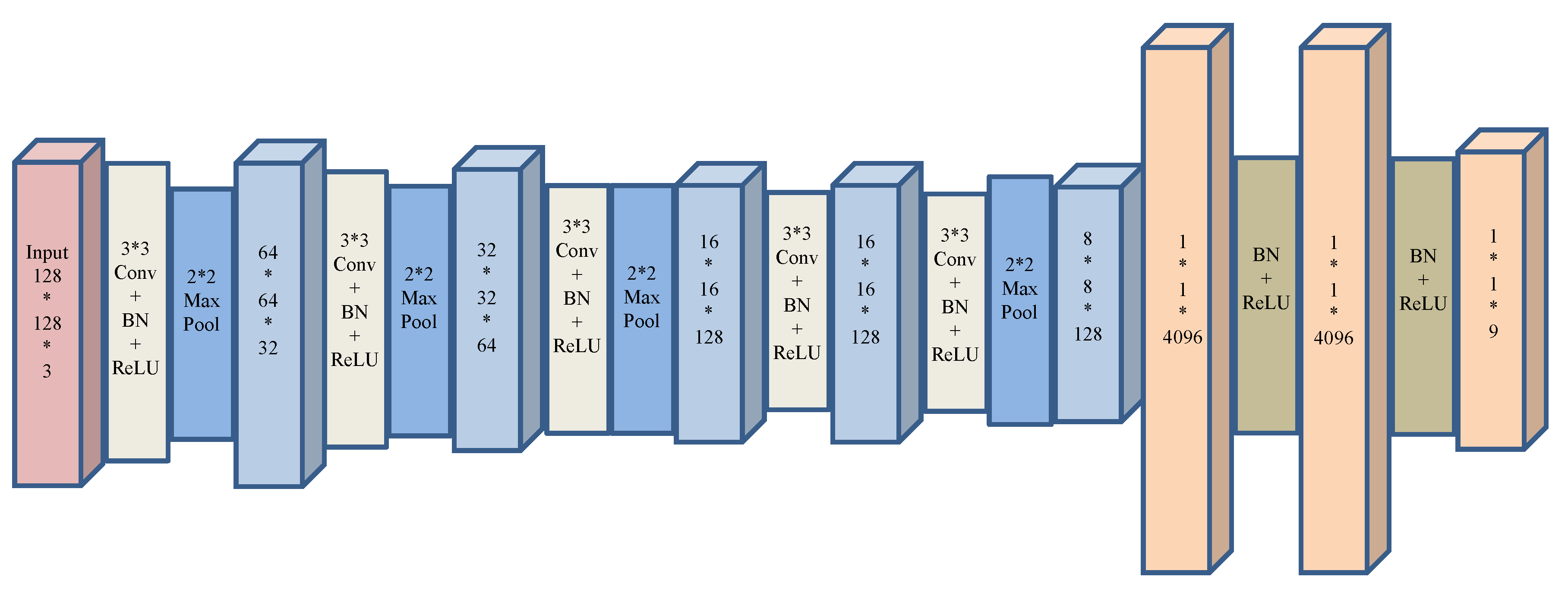
The architecture of the used CNN model is shown in Figure 2. We implemented the CNN using Caffe deep learning networks [24]. A CNN is usually composed of convolutional layers and pooling layers (denoted as Conv and pool here). These layers can help the network extract hierarchical features from the original inputs, followed by several fully connected layers (denoted as FC here) to perform the classification.
Considering a CNN with K layers, we denote the kth output layer as , where and the input data are denoted as . In each layer, there are two parts of the parameters for us to train, of which the weight matrix connects the previous layer with and the bias vector .
As shown in Figure 2, the input data is usually followed with the convolution layer. The convolution layer first performs a convolution operation with the kernels . Then, we add the bias vector with the resulting feature maps. After obtaining the features, a pointwise non-linear activation operation is usually performed subsequently. The size of the convolution kernels in our model is 3 × 3. A pooling layer (e.g., taking the average or maximum of adjacent locations) is followed, which uses the non-overlapping square windows per feature map to select the dominant features. The pooling layer can reduce the number of network parameters and improve the robustness of the translation. This layer offers invariance by reducing the resolution of the feature maps, and each pooling layer corresponds to the previous convolutional layer. The neuron in the pooling layer combines a small N × 1 patch of the convolution layer. The most common pooling operation is max pooling, which we chose for our experiments. The entire process can be formulated as
denotes the convolution operator and pool denotes the pooling operator.
The hierarchical feature extraction architecture is formed by stacking several convolution layers and pooling layers one by one. Then, we combine the resultant features with the 1D features using the FC layer. A fully connected layer takes all neurons in the previous layer and connects them to every single neuron contained in the layer. It first processes its inputs with a linear transformation by the weight and the bias vector , and then, the pointwise non-linear activation is performed as follows:
For the non-linear activation operation , we use rectified linear units. Unlike binary units, the rectified linear units (ReLU) [25] preserve information about the relative intensities as information travels through multiple layers of features detectors. It uses a fast approximation where the sampled value of the rectified linear unit is not constrained to be an integer. The function can be written as
Training deep neural networks is complicated by the distribution of each layer’s inputs during the training. Batch Normalization (BN) [26] allows us to use much higher learning rates, to be less careful about initialization, and to prevent overfitting. Consider a mini-batch B of size m . The BN transform is performed as follows:
and are parameters to be learned and is a constant added for numerical stability.
The last classification layer is always a softmax layer, with the number of neurons equaling the number of classes to be classified. Using a logistic regression layer with one neuron to perform binary classification, the activation value represents the probability that the input belongs to the positive class. The softmax layer guarantees that the output is a probability distribution, as the value for each label is between 0 and 1 and all the values add up to 1. The multi-label problem is then seen as a regression on the desired output label vectors.
If there is a set T of all possible classes, for the n training samples , the loss function L quantifies the misclassification by comparing the target label vectors and the predicted label vectors . We use the common cross-entropy loss in this work, which is defined as
The cross-entropy loss is numerically stable when coupled with the softmax normalization [27] and has a fast convergence rates when training neural networks.
When the loss function is defined, the model parameters that minimize the loss should be solved. The model parameters are composed by the weights and the biases . The back propagation algorithm is widely used to optimize these parameters. It propagates the prediction error from the last layer to the first layer and optimize the parameters according to the propagated error at each layer. The derivative of the parameters W and b can be described as and , respectively. The loss function can be optimized from the gradient of the parameters.
2.2. Feature Image Generation
To match the CNN with our ALS data, a feature image-generation method was proposed. In Hu’s method, each point Pk and its surrounding points within a “square window” were divided into 128 × 128 cells. The height relations among all the points within the cell are obtained and used to generate images which are then used to train the CNN model. This area-based feature image-generation method performed well in the DTM-generation task. However, the method may have problems when facing the multi-objects semantic labeling task. Objects such as trees and roofs are difficult to distinguish, so we proposed a single point-based feature image-generation method.
Like Hu’s method, we set up a square window for each ALS point (coordinates are , and ) and divide the window into 128 × 128 cells. Based on the ALS dataset we choose the width of the cell to be . For each cell, instead of using the height relations between all points, we choose a unique point and calculate the point based features. To find this unique point, we first need to calculate the center coordinate of the cell. The coordinates , and are calculated as follows:
i denotes the row number, j denotes the column number and is the width of the cell.
The unique point is the nearest point from the center. We calculate three types of features based on this point, which are the local geometric features, global geometric features and full-waveform LiDAR features as follows:
- (1)
- We calculate the local geometric features. All the features are extracted in a sphere of radius r. For a point , based on its n neighboring points, we obtain a center of gravity . We then calculate the vector . The variance–covariance matrix is written as
- (2)
Chehata [6] confirmed that is the most important eigenvalue. The planar objects such as roofs and roads have low values in , while non-planar objects have high values. Therefore in planar objects, the planarity is represented with high values. In contrast, the sphericity gives high values for an isotropically distributed 3D neighborhood. These two features help to distinguish planar objects such as roofs, façades, and roads easily from objects such as vegetation and cars.
The planarity of the local neighborhood is also the local geometric feature that will help discriminate buildings from vegetation. The local plane ΠP is estimated using a robust M-estimator with norm [29]. For each point, we obtain a normal vector from the plane. Then, the angle between the normal vector and the vertical direction can be calculated. We can obtain several angles from the neighboring points within a sphere of radius r. Using the variance of these angles helps us to discriminate planar surfaces such as roads from vegetation.
- (1)
- We extract the global geometric features. We generate the DTM for the feature height above DTM based on robust filtering [30], which is implemented in the commercial software package SCOP++. The height above DTM represents the global distribution for a point and helps to classify the data. Based on the analysis by Niemeyer [15], this feature is by far the most important since it is the strongest and most discernible feature for all the classes and relations. For instance, this feature has the capability to distinguish between a relation of points on a roof or on a road level.
- (2)
After calculating the features from the point , we then transfer these features into three integers from 0 to 255 as follows:
and are normalized between 0 and 1 and are the eigenvalue-based features, is normalized between 0 and 1 and is the variance of the normal vector angle from the vertical direction, is the normalized height above DTM between 0 and 1, and Intensity is the echo intensity value normalized between 0 and 255.
For each cell, the RED, GREEN and BLUE are mapped to a pixel with red, blue and green colors. Then, the square window can be transferred to a 128 × 128 image. The steps of the feature image generation are shown in Figure 3.
The spatial context of the point is successfully transferred into an image by the distribution of point and its three types of features. The CNN model extracts the high-level representations through these limited low-level feature images and performs well in the ALS point clouds semantic labeling task.
2.3. Accuracy Evaluation
According to the benchmark rules, the overall accuracy and F1 score are used to assess the performance of our resulting values. In the benchmark, the tp, fp and fn are true positive, false positive and false negative, respectively, and can be calculated using pixel-based confusion matrices per tile or an accumulated confusion matrix. In each class, we compute the precision and recall as follows:
Then, the F1 score is calculated as
The overall accuracy is the normalization of the trace from the confusion matrix.
3. Experimental Result
3.1. Dataset
We evaluate the proposed method on the ISPRS 3D semantic labeling contest [32], which is an open benchmark dataset. The dataset that we use is acquired with the Leica ALS50 system over Vaihigen, a small village in Germany [33]. This dataset has been presented in the scope of the ISPRS Test Project on Urban Classification and 3D Building Reconstruction and simultaneously serves as the benchmark dataset for the ISPRS benchmarks on 2D and 3D semantic labeling. The ALS50 system has a mean flying height of 500 m above ground and a 45 degrees field of view. The point density in the test area is approximately 8 points/m2. For the 3D semantic labeling, nine classes have been defined and each point in the dataset is labeled accordingly. The reference labels are provided by the authors of [15].
The given area is subdivided into two parts. The first area is treated as a training set and has 753,876 labeled points. Nine semantic classes have been defined for the Vaihingen dataset, which are the power-line, low vegetation, impervious surfaces, car, fence/hedge, roof, façade, shrub, and tree. The second area is treated as the testing set and has 411,722 unlabeled points. The training set is visualized in Figure 4a and contains the spatial XYZ-coordinates, intensity values, the number of returns, and the reference labels. The test set is shown in Figure 4b, and only the spatial XYZ-coordinates, intensity values and the number of returns are provided. More detailed information is shown in Table 1.
3.2. Experiments
The experiments focus on using the presented local geometric features, global geometric features and full-waveform features (Section 2.2) to generate the feature images. Then, these feature images serve as the input for a CNN to perform the 3D semantic task (Section 2.1).
The unbalanced distribution of the training examples per class cloud have a detrimental effect on the training process [34]. As a result, we use a class re-balancing method by randomly sampling the training example to obtain the final training set. As shown in Table 1, we reduce the values of any point numbers of the classes that are larger than 15,000. Classes such as the Powerline and Car have point numbers of less than 15,000, so those values remain unmodified.
The batch gradient descent with a batch size of 128 examples, base learning rate of 0.01, momentum of 0.9, and weight decay of 0.0005 to estimate the CNN parameters is used for training. The training of the CNN model is performed on a PC with an NVIDIA Tesla K20c.
We first use the five features that were discussed in Section 2.2 and set the width of cell 0.05 m. Then, we consider the influence of the radius for the spherical neighborhood:
- R0.5 indicates a radius of 0.5 m;
- R0.75 indicates a radius of 0.75 m;
- R1.0 indicates a radius of 1.0 m;
- R2.0 indicates a radius of 2.0 m;
The result for the influence of the radius is shown in Table 2.
Then we use the five features and set the neighborhood radius to 1 m to determine the influence of the cell width:
- W0.025 indicates a cell width of 0.025 m;
- W0.05 indicates a cell width of 0.05 m;
- W0.075 indicates a cell width of 0.075 m;
- W0.1 indicates a cell width of 0.1 m;
- W0.2 indicates a cell width of 0.2 m.
The result for the influence of the cell width is shown in Table 3.
Finally, we set the neighborhood radius to 1 m and the cell width to 0.05 m to discuss the influence of the selected feature:
- In the CNN_DEIV, we use all five features that were discussed in Section 2.2, D represents using the feature height above DTM , E represents using the two eigenvalue-based features and , I represents using the feature , and V represents using the feature variance of normal vector angle from vertical direction .
- In the CNN_GEIV, all the features we use are the same as the CNN_DEIV except for the feature height above DTM . G indicates that we add some Gaussian noise to the DTM.
- In the CNN_LEIV, all the features we use are the same as the CNN_DEIV except for the feature height above DTM . L indicates that we use the low accuracy DTM to replace the DTM in the CNN_DEIV.
- In the CNN_DEI, all the features we use are the same as the CNN_DEIV except for the feature variance of normal vector angle from vertical direction , which is removed from the Equation (10).
- In the CNN_EI, all the features we use are the same as the CNN_DEI except for the feature height above DTM , which is removed from the Equation (10) and replaced with the relative height difference. This feature is calculated from the difference between the height of a point and the average height value in its neighborhood.
- In the CNN_E, all the features we use are the same as the CNN_EI except for the feature , which is removed from the Equation (10) and replaced with the integer 255.
The result of influence of the different features is shown in Table 4, and the visualization of our best result CNN_DEIV is shown in Figure 5.
We use all five features and set the neighborhood radius to 1 m, set the cell width to 0.05 m, and then change the training samples:
- Sall uses all the samples to train the CNN model;
- Sreb uses re-balanced samples shown in Table 1;
- Srep repeats the sparser classes in Sreb that makes all the classes have 15,000 samples.
The results are shown in Table 5.
3.3. ISPRS Benchmark Testing Results
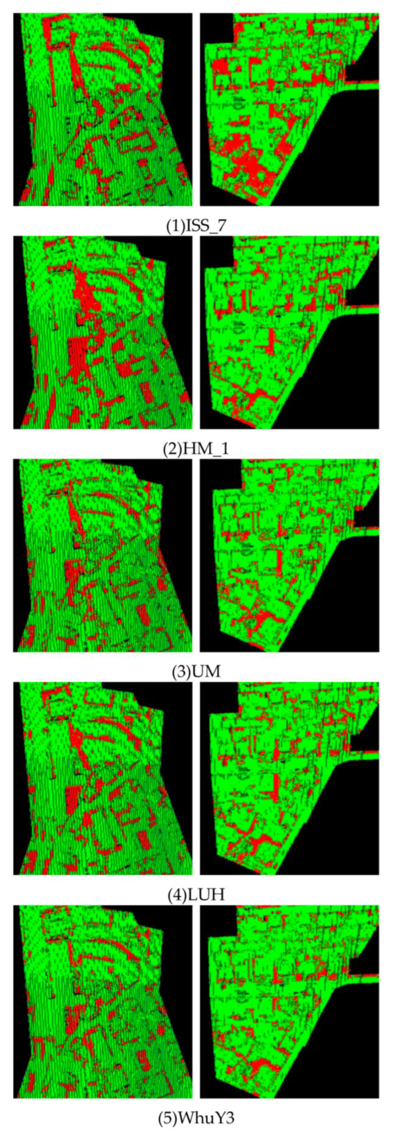
We submitted the CNN_DEIV result on the unlabeled test data to the ISPRS organizers for evaluation. As shown in Table 6, we provided the precision for five main classes, recall and F1 values accompanied with the overall accuracy of all nine classes. These five classes occupy 89% of the test set and are the key factor affecting the overall accuracy. Our method is WhuY3 (identical to CNN_DEIV). The ISS_7 [35] uses supervoxels-based segmentation to segment the point cloud data and uses a machine-learning algorithm to label the points. The HM_1 [36] uses conditional random fields (CRF) to perform the semantic analysis of the ALS data. The UM [37] uses a genetic algorithm based on the features extracted from the LiDAR point-attributes, textural analysis, and geometric attributes for the 3D semantic labeling. The LUH [38] uses hierarchical conditional random fields (HCRF) for the classification. The visual performance among the related methods is shown in Figure 6.
4. Discussion
There are three main parameters in our work: the neighborhood radius, the cell width, and the feature selection. To determine the impact of the parameters on the classification result, we perform three successive experiments in which we treat each parameter independently and show its influence on all nine classes.
For the radius selection (Table 2), we choose four different radii from 0.5 m to 2.0 m. In general, the overall accuracy and the average F1 have the highest value when the radius is 1 m. More specifically, since the point density of each class is different, as the radius increases, the recall value of the power line reduces, the recall values of the façade and shrub increase, and the recall values of the other classes increase initially and then decrease. Although the radius of the neighborhoods does have some influence on the classification, the overall accuracy and the average F1 of all radii show a relatively good performance at approximately 81 and 61. This is because our method uses the features from the point itself and the features from its surrounding cells. This neighborhood information may somehow reduce the importance of the radius selection. Taking the overall accuracy and the average F1 into consideration, we choose the radius of 1 m in the following experiments.
For the cell width selection (Table 3), we choose five different widths from 0.025 m to 0.2 m. Since our method reconstructs the feature distribution around a point to an image, the width of the cell is an important parameter in our framework. When the width is short, some objects, such as power line, fence/hedge and shrubs, appear to have a higher recall value. In the meantime, the recall values of the low vegetation, impervious surfaces and roof are lower. When the width is long, the roof recall value has the best performance, but leads to significant loss in the tree and shrub values. Taking the overall accuracy and the average F1 into consideration, we choose a width of 0.05 m in the following experiments.
We replace or reduce the features in the CNN_DEIV to determine the influence of each feature (Table 4). When some Gaussian noise is added to our DTM, indicated by CNN_GEIV, the overall accuracy and the average F1 are slightly reduced. Therefore, our method has the ability to handle noise in the DTM to some extent due to the point-based feature image generation. However, when the accuracy of the DTM is low, as shown in CNN_LEIV, the results are not satisfactory. The recall values of the low vegetation, impervious surface and roof all reduce. This may be due to ambiguities, since these objects have a similar planar behavior. The same results appear when comparing the CNN_DEI with the CNN_EI. Thus, we may state that the performance of the proposed method depends significantly on the quality of the DTM. The overall accuracy and the average F1 are relatively low in CNN_E. It is difficult to solve the misclassification of low vegetation and impervious surface using only the eigenvalue-based features and , so we add the feature as indicated by CNN_EI. In this case, the recall value of the low vegetation and impervious surface improves sharply. Although the CNN_DEI performs well enough, the recall value of the cars (47.5%) is still relatively low. Therefore, we add the feature variance of normal vector angle from vertical direction which successfully solves the problem (+21.8%). After these experiments, we find the proper values of the three parameters, showing that the end results of our method CNN_DEIV perform well on overall accuracy (82.3%) and average F1 (61.6%).
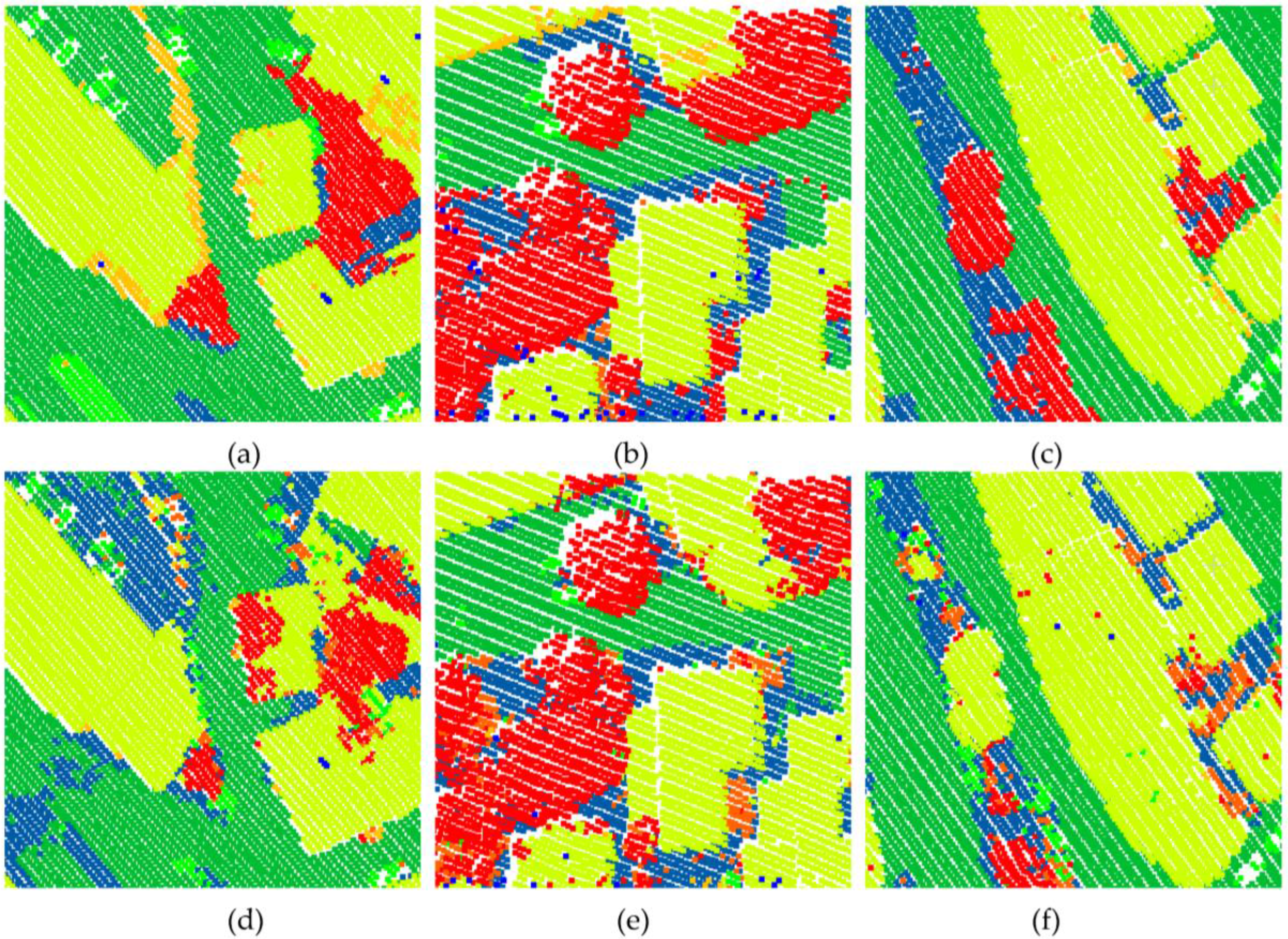
Our method has a satisfactory performance when compared with all the participants on the ISPRS WG II/4 Vaihingen 3D Semantic Labeling task. The overall accuracy of our method is ranked 1st, and the average F1 of the five main categories is ranked 2nd, for all the participants. Since the overall accuracy is high, our method has the lowest proportion of red in Figure 6. It should be noted that only five features are used in our final experiment, and the existing methods rely on several features for the LiDAR points and the interaction of the neighboring points. For example, in the LUH [38], Niemeyer used 35 elements in his feature vector. The convolutional networks exploit the potential of the selected features as we expected. At the same time, the low quantities of the features may lead to some misclassifications. Some objects, such as the powerline, fence/hedge and shrubs have relatively low F1 scores. There also some faults in five main categories. We compare our method with the ground truth, and Figure 7 shows some failure classification from our method. In these areas, roofs are yellow, trees are red, impervious surfaces are green, low vegetation is blue, and the cars are lime. We can see that some trees and roofs are difficult to distinguish, some cars are wrongly classified as low vegetation, and some impervious and low vegetation are mixed together. The unusual distribution of points and the point density cause these misclassifications. Choosing the features, such as height variance, echo features, point density and hierarchical features, that other methods used during our image-generation process may improve the accuracy in similar cases. In addition, using the eigen-entropy maximization in the neighborhood selection portion as Weinmann [9] did, may also improve the results.
In our framework, each point in the data is transferred into an image. Some points are close enough to have the same feature images. Although we have taken the point spatial correlation into consideration, there are still a few noisy points in our labeling result (Figure 7). In addition, generating the feature image for each point can be resource-intensive and time-consuming, and the computational effort in the CNN is high with a long training period (Table 5). We can use a pre-segmentation technique, as Guninard [39] did, to reduce the computation burden. This process divides the point clouds into smaller, connected subsets with sizes determined by the local complexity. This helps to cope with the labeling noise and to reduce the number of feature images, which may help to address our problems.
5. Conclusions
In this paper, we propose a point-based feature image-generation method used by a CNN model for ALS data semantic labeling. For each point in the ALS data, we generate the image based on the features of its neighboring points. Then, a deep CNN model is used to train and classify the feature images. Each point can be classified into nine categories by the deep CNN model. Experiments on the ISPRS dataset confirm the capabilities of the proposed method compared with state-of-the-art methods. As shown in Table 6, the overall accuracy ranks 1st and the average F1 ranks 2nd compared with the other considered approaches.
Our method still has the potential for improvement given that only five features are used in our final experiment. There is a lot of work to do on the feature image-generation process, such as using different kinds of features and choosing the optimal neighborhood. In future work, we will take elements such as the height variance, echo features, point density, and hierarchical features into consideration, and use a more robust optimal neighborhood, to further improve the performance and to apply a segment-based method into our framework in order to reduce the computational burden and time. In addition, we will also try to apply our model to more complex 3D segmentation tasks.
Acknowledgments
The labeled data was provided by Joachim Niemeyer, Institute of Photogrammetry and GeoInformation, Leibniz Universität Hannover, Nienburger Str. 1, D-30167 Hannover, Germany. The partial evaluations of results were provided by Markus Gerke, Utwente/ITC/EOS.
Author Contributions
Zhishuang Yang and Wanshou Jiang contributed to the study design and manuscript writing; Zhishuang Yang and Bo Xu conceived and designed the experiments; Zhishuang Yang performed the experiments; Quansheng Zhu and San Jiang contributed to the initial data and the analysis tools; and Wei Huang contributed to partial codes of the algorithm.
Conflicts of Interest
The authors declare no conflict of interest.
References
- Bishop, C.M. Pattern Recognition and Machine Learning (Information Science and Statistics); Springer: New York, NY, USA, 2006; p. 049901. [Google Scholar]
- Chan, C.W.; Paelinckx, D. Evaluation of random forest and adaboost tree-based ensemble classification and spectral band selection for ecotope mapping using airborne hyperspectral imagery. Remote Sens. Environ. 2008, 112, 2999–3011. [Google Scholar] [CrossRef]
- Mountrakis, G.; Im, J.; Ogole, C. Support vector machines in remote sensing: A review. ISPRS J. Photogramm. Remote Sens. 2011, 66, 247–259. [Google Scholar] [CrossRef]
- Breiman, L. Random forests. Mach. Learn. 2001, 45, 5–32. [Google Scholar] [CrossRef]
- Gislason, P.O.; Benediktsson, J.A.; Sveinsson, J.R. Random forests for land cover classification. Pattern Recognit. Lett. 2003, 27, 294–300. [Google Scholar] [CrossRef]
- Chehata, N.; Li, G.; Mallet, C. Airborne LiDAR feature selection for urban classification using random forests. Geomat. Inf. Sci. Wuhan Univ. 2009, 38, 207–212. [Google Scholar]
- Mallet, C. Analysis of Full-Waveform LiDAR Data for Urban Area Mapping. Ph.D Thesis, Télécom ParisTech, Paris, France, 2010. [Google Scholar]
- Mallet, C.; Bretar, F.; Roux, M.; Soergel, U.; Heipke, C. Relevance assessment of full-waveform LiDAR data for urban area classification. ISPRS J. Photogramm. Remote Sens. 2011, 66, S71–S84. [Google Scholar] [CrossRef]
- Weinmann, M.; Jutzi, B.; Hinz, S.; Mallet, C. Semantic point cloud interpretation based on optimal neighborhoods, relevant features and efficient classifiers. ISPRS J. Photogramm. Remote Sens. 2015, 105, 286–304. [Google Scholar] [CrossRef]
- Geman, S.; Geman, D. Stochastic relaxation, Gibbs distributions, and the Bayesian restoration of images. IEEE Trans. Pattern Anal. Mach. Intell. 1984, 6, 721–741. [Google Scholar] [CrossRef] [PubMed]
- Kumar, S.; Hebert, M. Discriminative random fields. Int. J. Comput. Vis. 2006, 68, 179–201. [Google Scholar] [CrossRef]
- Anguelov, D.; Taskarf, B.; Chatalbashev, V.; Koller, D.; Gupta, D.; Heitz, G.; Ng, A. In discriminative learning of Markov random fields for segmentation of 3D scan data. In Proceedings of the Computer Vision and Pattern Recognition, San Diego, CA, USA, 20–25 June 2005. [Google Scholar]
- Shapovalov, R.; Velizhev, A.; Barinova, O. Non-associative Markov networks for 3D point cloud classification. Int. Arch. Photogramm. Remote Sens. Spat. Inf. Sci. 2010, XXXVIII, 103–108. [Google Scholar]
- Rusu, R.B.; Holzbach, A.; Blodow, N.; Beetz, M. Fast geometric point labeling using conditional random fields. In Proceedings of the Intelligent Robots and Systems, St. Louis, MO, USA, 10–15 October 2009. [Google Scholar]
- Niemeyer, J.; Rottensteiner, F.; Soergel, U. Contextual classification of LiDAR data and building object detection in urban areas. ISPRS J. Photogramm. Remote Sens. 2014, 87, 152–165. [Google Scholar] [CrossRef]
- LeCun, Y.; Boser, B.; Denker, J.S.; Henderson, D.; Howard, R.E.; Hubbard, W.; Jackel, L.D. Backpropagation applied to handwritten zip code recognition. Neural Comput. 1989, 1, 541–551. [Google Scholar] [CrossRef]
- Krizhevsky, A.; Sutskever, I.; Hinton, G.E. Imagenet classification with deep convolutional neural networks. In Proceedings of the Neural Information Processing Systems Conference, Lake Tahoe, NV, USA, 3–8 December 2012. [Google Scholar]
- Simonyan, K.; Zisserman, A. Very Deep Convolutional Networks for Large-Scale Image Recognition. Available online: https://arxiv.org/abs/1409.1556 (accessed on 8 September 2017).
- Szegedy, C.; Liu, W.; Jia, Y.; Sermanet, P. Going deeper with convolutions. In Proceedings of the IEEE Conference on Computer Vision and Pattern Recognition, Boston, MA, USA, 8–10 June 2015. [Google Scholar]
- Girshick, R.; Donahue, J.; Darrell, T.; Malik, J. Rich feature hierarchies for accurate object detection and semantic segmentation. In Proceedings of the IEEE Conference on Computer Vision and Pattern Recognition, Columbus, OH, USA, 24–27 June 2014. [Google Scholar]
- Boulch, A.; Saux, B.L.; Audebert, N. Unstructured point cloud semantic labeling using deep segmentation networks. In Eurographics Workshop on 3D Object Retrieval; The Eurographics Association: Geneva, Switzerland, 2017. [Google Scholar] [CrossRef]
- Hackel, T.; Wegner, J.D.; Schindler, K. Fast semantic segmentation of 3D point clouds with strongly varying density. ISPRS Ann. Photogramm. Remote Sens. Spat. Inf. Sci. 2016, 3, 177–187. [Google Scholar] [CrossRef]
- Hu, X.; Yuan, Y. Deep-learning-based classification for DTM extraction from ALS point cloud. Remote Sens. 2016, 8, 730. [Google Scholar] [CrossRef]
- Jia, Y.; Shelhamer, E.; Donahue, J.; Karayev, S.; Long, J.; Girshick, R.; Guadarrama, S.; Darrell, T. Caffe: Convolutional architecture for fast feature embedding. In Proceedings of the 22nd ACM International Conference on Multimedia, Orlando, FL, USA, 3–7 November 2014. [Google Scholar]
- Nair, V.; Hinton, G.E. Rectified linear units improve restricted boltzmann machines. In Proceedings of the 27th International Conference on Machine Learning, Haifa, Israel, 21–24 June 2010. [Google Scholar]
- Ioffe, S.; Szegedy, C. Batch normalization: Accelerating deep network training by reducing internal covariate shift. In Proceedings of the 32nd International Conference on Machine Learning, Lile, France, 6–11 July 2015. [Google Scholar]
- Bishop, C.M. Neural Networks for Pattern Recognition; Oxford University Press: Oxford, UK, 1995. [Google Scholar]
- Demantké, J.; Mallet, C.; David, N.; Vallet, B. Dimensionality based scale selection in 3D LiDAR point clouds. ISPRS Int. Arch. Photogramm. Remote Sens. Spat. Inf. Sci. 2011, 38, W12. [Google Scholar] [CrossRef]
- Xu, G.; Zhang, Z. Epipolar geometry in stereo, motion and object recognition. Comput. Imaging Vis. 1996, 6. [Google Scholar] [CrossRef]
- Kraus, K.; Pfeifer, N. Determination of terrain models in wooded areas with airborne laser scanner data. ISPRS J. Photogramm. Remote Sens. 1998, 53, 193–203. [Google Scholar] [CrossRef]
- Wagner, W.; Ullrich, A.; Ducic, V.; Melzer, T.; Studnicka, N. Gaussian decomposition and calibration of a novel small-footprint full-waveform digitising airborne laser scanner. ISPRS J. Photogramm. Remote Sens. 2006, 60, 100–112. [Google Scholar] [CrossRef]
- International Society for Photogrammetry and Remote Sensing. 3D Semantic Labeling Contest. Available online: http://www2.isprs.org/commissions/comm3/wg4/3d-semantic-labeling.html (accessed on 8 September 2017).
- Cramer, M. The DGPF-test on digital airborne camera evaluation—Overview and test design. Photogramm. Fernerkund. Geoinf. 2010, 2010, 73–82. [Google Scholar] [CrossRef] [PubMed]
- Chen, C.; Breiman, L. Using Random Forest to Learn Imbalanced Data; 666; University of California, Berkeley: Berkeley, CA, USA, 2004. [Google Scholar]
- Ramiya, A.M.; Nidamanuri, R.R.; Ramakrishnan, K. A supervoxel-based spectro-spatial approach for 3d urban point cloud labelling. Int. J. Remote Sens. 2016, 37, 4172–4200. [Google Scholar] [CrossRef]
- Steinsiek, M.; Polewski, P.; Yao, W.; Krzystek, P. Semantische analyse von ALS- und MLS-daten in urbanen gebieten mittels conditional random fields. In Proceedings of the 37. Wissenschaftlich-Technische Jahrestagung der DGPF, Würzburg, Germany, 8–10 March 2017. [Google Scholar]
- Horvat, D.; Žalik, B.; Mongus, D. Context-dependent detection of non-linearly distributed points for vegetation classification in airborne lidar. ISPRS J. Photogramm. Remote Sens. 2016, 116, 1–14. [Google Scholar] [CrossRef]
- Niemeyer, J.; Rottensteiner, F.; Soergel, U.; Heipke, C. Hierarchical higher order crf for the classification of airborne lidar point clouds in urban areas. ISPRS Int. Arch. Photogramm. Remote Sens. Spat. Inf. Sci. 2016, XLI-B3, 655–662. [Google Scholar] [CrossRef]
- Guinard, S.; Landrieu, L. Weakly supervised segmentation-aided classification of urban scenes from 3D lidar point clouds. In Proceedings of the ISPRS Workshop 2017, Hannover, Germany, 6–9 June 2017. [Google Scholar]
Figure 1.
The workflow of the proposed method.
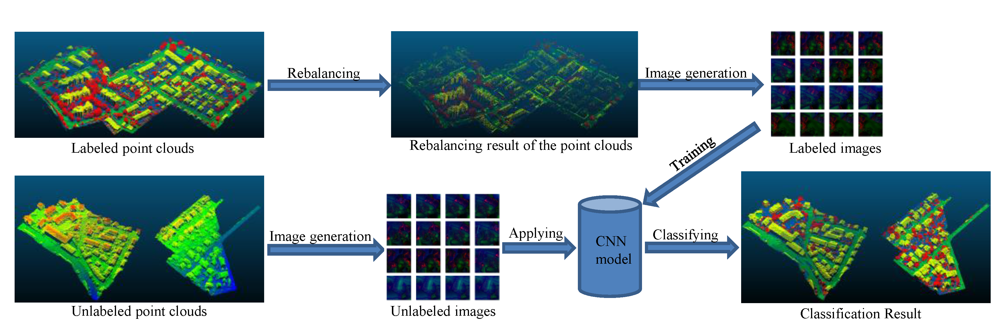
Figure 2.
The architecture of the deep CNN used.

Figure 3.
Steps of the feature image generation.
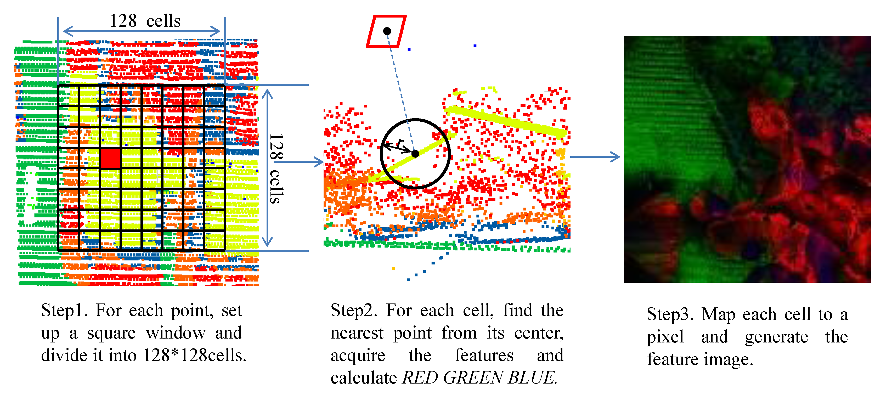
Figure 4.
(a) The training set: the color encoding shows the assigned semantic class labels (Powerline: blue; Low Vegetation: Navy; Impervious Surfaces: green; Car: lime; Fence/Hedge: lawngreen; Roof: yellow; Façade: gold; Shrub: orange; Tree: red). (b) The testing set: The colors blue to red represent the z values of the points.
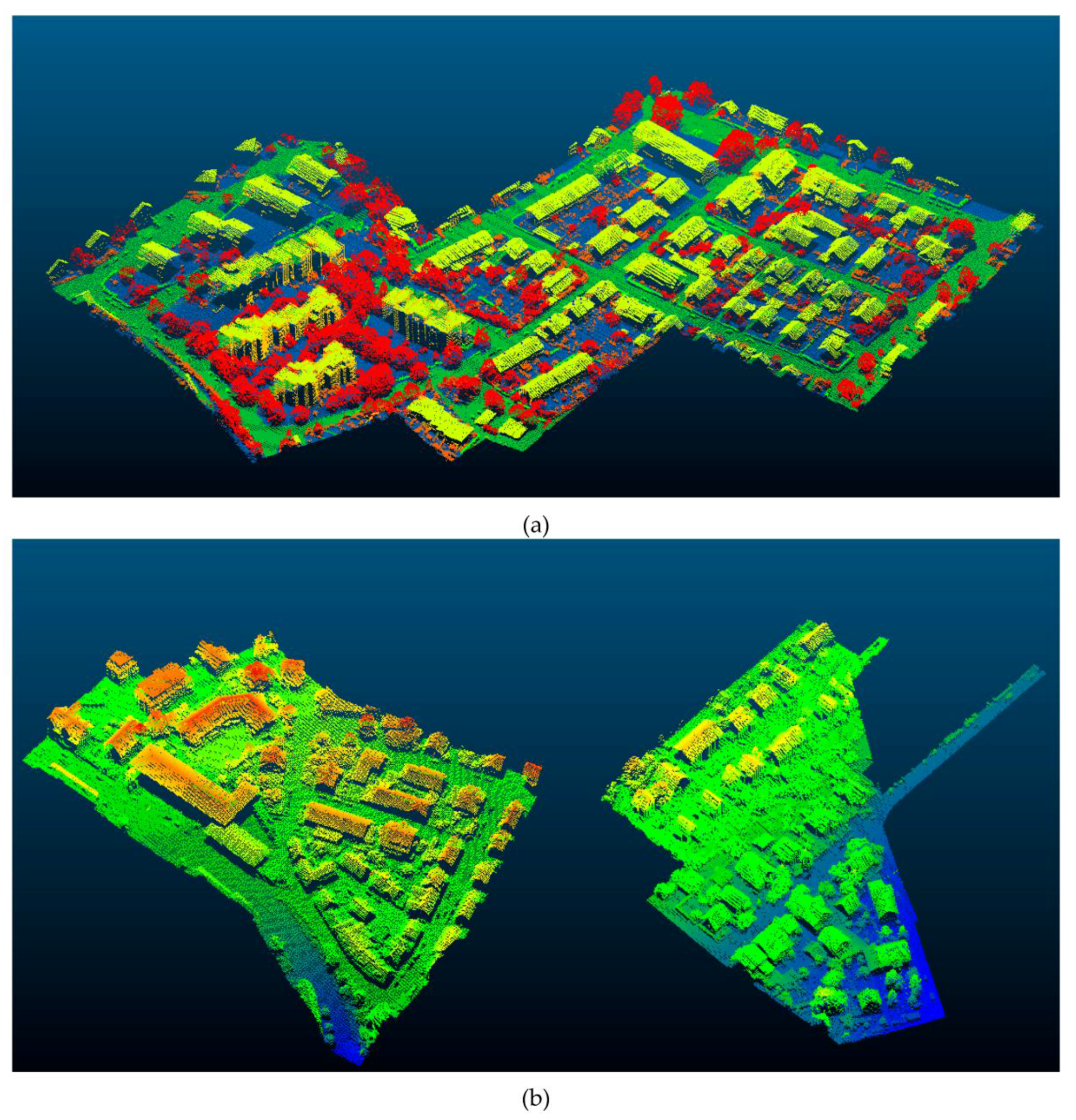
Figure 5.
The classification result of the CNN_DEIV.
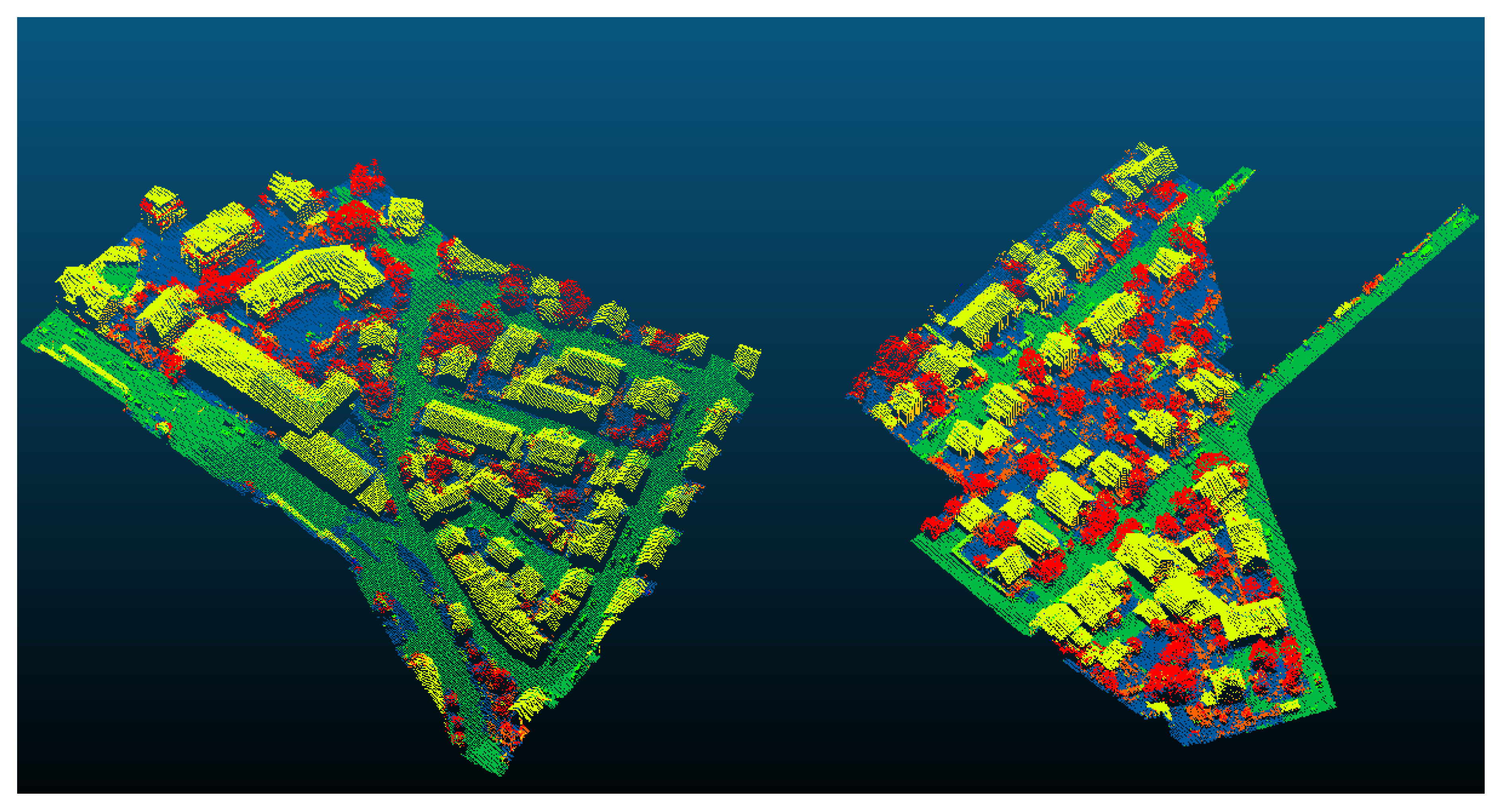
Figure 6.
Visual performance among related methods. Green represents the true classification results, and red represents the false classification results.
Figure 6.
Visual performance among related methods. Green represents the true classification results, and red represents the false classification results.

Figure 7.
Failure classification. (a–c) are the ground results, while (d–f) are the corresponding WhuY3 result.
Figure 7.
Failure classification. (a–c) are the ground results, while (d–f) are the corresponding WhuY3 result.

Table 1.
Number of 3D points per class.
| Class | Training Set | Training Set Used | Test Set |
|---|---|---|---|
| Powerline | 546 | 546 | N/A |
| Low Vegetation | 180,850 | 18,005 | N/A |
| Impervious Surfaces | 193,723 | 19,516 | N/A |
| Car | 4614 | 4614 | N/A |
| Fence/Hedge | 12,070 | 12,070 | N/A |
| Roof | 152,045 | 15,235 | N/A |
| Façade | 27,250 | 13,731 | N/A |
| Shrub | 47,605 | 11,850 | N/A |
| Tree | 135,173 | 13,492 | N/A |
| ∑ | 753,876 | 109,059 | 411,722 |
Table 2.
The recall value, the overall accuracy of each class and average F1 value for different neighborhood radii in (%). Bold numbers show the highest values within the different radii.
Table 2.
The recall value, the overall accuracy of each class and average F1 value for different neighborhood radii in (%). Bold numbers show the highest values within the different radii.
| Class | R0.5 | R0.75 | R1.0 | R2.0 |
|---|---|---|---|---|
| Power | 31.3 | 26.1 | 24.7 | 20.3 |
| Low Vegetation | 80.2 | 80.9 | 81.8 | 81.2 |
| Impervious Surfaces | 87.8 | 90.2 | 91.9 | 89.2 |
| Car | 59.3 | 71.2 | 69.3 | 64.2 |
| Fence/Hedge | 11.2 | 12.7 | 14.7 | 13.6 |
| Roof | 93.1 | 94.4 | 95.4 | 94.9 |
| Façade | 34.1 | 38.1 | 40.9 | 41.7 |
| Shrub | 36.4 | 37.7 | 38.2 | 38.3 |
| Tree | 77.5 | 77.9 | 78.5 | 78.1 |
| Overall Accuracy | 79.7 | 81.2 | 82.3 | 81.3 |
| Average F1 | 60.5 | 61.3 | 61.6 | 60.7 |
Table 3.
The recall value, the overall accuracy of each class and the average F1 value for different cell widths in (%). Bold numbers show the highest values within different features.
Table 3.
The recall value, the overall accuracy of each class and the average F1 value for different cell widths in (%). Bold numbers show the highest values within different features.
| Class | W0.025 | W0.05 | W0.075 | W0.1 | W0.2 |
|---|---|---|---|---|---|
| Power | 28.4 | 24.7 | 22.1 | 19.3 | 15.1 |
| Low Vegetation | 78.6 | 81.8 | 81.9 | 81.7 | 80.4 |
| Impervious Surfaces | 90.2 | 91.9 | 90.4 | 88.6 | 83.6 |
| Car | 66.7 | 69.3 | 62.1 | 59.3 | 53.2 |
| Fence/Hedge | 18.3 | 14.7 | 14.3 | 10.9 | 9.5 |
| Roof | 93.1 | 95.4 | 95.5 | 95.8 | 96.3 |
| Façade | 40.2 | 40.9 | 35.9 | 36.3 | 39.3 |
| Shrub | 39.1 | 38.2 | 35.7 | 30.4 | 20.1 |
| Tree | 76.6 | 78.5 | 78.9 | 69.3 | 66.8 |
| Overall Accuracy | 80.4 | 82.3 | 81.7 | 79.6 | 77.2 |
| Average F1 | 62.4 | 61.6 | 61.2 | 60.1 | 57.3 |
Table 4.
The recall value, the overall accuracy of each class and the average F1 value for different feature selections in (%). Bold numbers show the highest value within the different features.
Table 4.
The recall value, the overall accuracy of each class and the average F1 value for different feature selections in (%). Bold numbers show the highest value within the different features.
| Class | CNN_DEIV | CNN_GEIV | CNN_LEIV | CNN_DEI | CNN_EI | CNN_E |
|---|---|---|---|---|---|---|
| Power | 24.7 | 24.3 | 22.7 | 20.5 | 17.2 | 23.0 |
| Low Vegetation | 81.8 | 81.9 | 78.3 | 82.0 | 75.4 | 63.1 |
| Impervious Surfaces | 91.9 | 91.7 | 79.2 | 88.7 | 80.0 | 49.6 |
| Car | 69.3 | 69.1 | 58.7 | 47.5 | 46.8 | 32.1 |
| Fence/Hedge | 14.7 | 15.3 | 17.8 | 15.9 | 20.3 | 19.4 |
| Roof | 95.4 | 95.0 | 84.0 | 92.3 | 83.6 | 84.5 |
| Façade | 40.9 | 40.8 | 45.3 | 46.4 | 44.9 | 47.6 |
| Shrub | 38.2 | 37.9 | 36.3 | 43.9 | 38.4 | 36.0 |
| Tree | 78.5 | 78.7 | 80.1 | 79.7 | 85.9 | 84.9 |
| Overall Accuracy | 82.3 | 82.2 | 75.5 | 81.0 | 75.7 | 65.1 |
| Average F1 | 61.6 | 61.3 | 56.3 | 58.9 | 55.8 | 50.1 |
Table 5.
The training time, testing time, overall accuracy and average F1 of our method for different samples using the re-balancing method.
Table 5.
The training time, testing time, overall accuracy and average F1 of our method for different samples using the re-balancing method.
| Samples | Sall | Sreb | Srep |
|---|---|---|---|
| Training time (h) | 43.1 | 6.5 | 7.2 |
| Testing time (s) | 70.2 | 70.4 | 69.7 |
| Overall Accuracy (%) | 80.2 | 82.3 | 82.2 |
| Average F1 (%) | 60.7 | 61.6 | 62.1 |
Table 6.
Quantitative comparison between our method and other published methods on the ISPRS test set. Bold numbers show the highest values within different methods.
Table 6.
Quantitative comparison between our method and other published methods on the ISPRS test set. Bold numbers show the highest values within different methods.
| Class | Value | ISS_7 | HM_1 | UM | LUH | WHUY3 |
|---|---|---|---|---|---|---|
| Impervious Surfaces | Precision | 76.0 | 89.1 | 88.0 | 91.8 | 88.4 |
| Recall | 96.5 | 94.2 | 90.3 | 90.4 | 91.9 | |
| F1 | 85.0 | 91.5 | 89.1 | 91.1 | 90.1 | |
| Roof | Precision | 86.1 | 91.6 | 93.6 | 97.3 | 91.4 |
| Recall | 96.2 | 91.5 | 90.5 | 91.3 | 95.4 | |
| F1 | 90.9 | 91.6 | 92.0 | 94.2 | 93.4 | |
| Low Vegetation | Precision | 94.1 | 83.8 | 78.6 | 83.0 | 80.9 |
| Recall | 49.9 | 65.9 | 79.5 | 72.7 | 81.8 | |
| F1 | 65.2 | 73.8 | 79.0 | 77.5 | 81.4 | |
| Tree | Precision | 84.0 | 77.9 | 71.8 | 87.4 | 77.5 |
| Recall | 68.8 | 82.6 | 85.2 | 79.1 | 78.5 | |
| F1 | 75.6 | 80.2 | 77.9 | 83.1 | 78.0 | |
| Car | Precision | 76.3 | 51.4 | 89.6 | 86.4 | 58.4 |
| Recall | 46.7 | 67.1 | 32.5 | 63.3 | 69.3 | |
| F1 | 57.9 | 58.2 | 47.7 | 73.1 | 63.4 | |
| All five classes | Average Precision | 83.3 | 78.8 | 84.3 | 89.1 | 79.3 |
| Average Recall | 71.6 | 80.3 | 75.6 | 79.4 | 83.4 | |
| Average F1 | 74.9 | 79.1 | 77.1 | 83.8 | 81.3 | |
| All nine classes | Overall Accuracy | 76.2 | 80.5 | 80.8 | 81.6 | 82.3 |
© 2017 by the authors. Licensee MDPI, Basel, Switzerland. This article is an open access article distributed under the terms and conditions of the Creative Commons Attribution (CC BY) license (http://creativecommons.org/licenses/by/4.0/).
Share and Cite
MDPI and ACS Style
Yang, Z.; Jiang, W.; Xu, B.; Zhu, Q.; Jiang, S.; Huang, W. A Convolutional Neural Network-Based 3D Semantic Labeling Method for ALS Point Clouds. Remote Sens. 2017, 9, 936. https://doi.org/10.3390/rs9090936
AMA Style
Yang Z, Jiang W, Xu B, Zhu Q, Jiang S, Huang W. A Convolutional Neural Network-Based 3D Semantic Labeling Method for ALS Point Clouds. Remote Sensing. 2017; 9(9):936. https://doi.org/10.3390/rs9090936
Chicago/Turabian StyleYang, Zhishuang, Wanshou Jiang, Bo Xu, Quansheng Zhu, San Jiang, and Wei Huang. 2017. "A Convolutional Neural Network-Based 3D Semantic Labeling Method for ALS Point Clouds" Remote Sensing 9, no. 9: 936. https://doi.org/10.3390/rs9090936
Note that from the first issue of 2016, this journal uses article numbers instead of page numbers. See further details here.