A Modified Normalized Difference Impervious Surface Index (MNDISI) for Automatic Urban Mapping from Landsat Imagery


1
Key Laboratory of Digital Earth Science, Institute of Remote Sensing and Digital Earth (RADI), Chinese Academy of Sciences (CAS), Beijing 100094, China
2
Key Laboratory for Earth Observation of Hainan Province, Sanya 572029, China
3
Department of Geography, University of South Carolina, Columbia, SC 29208, USA
4
Geomatics College, Shandong University of Science and Technology, Qingdao 266590, China
*
Author to whom correspondence should be addressed.
Remote Sens. 2017, 9(9), 942; https://doi.org/10.3390/rs9090942
Submission received: 16 August 2017
/
Revised: 8 September 2017
/
Accepted: 8 September 2017
/
Published: 12 September 2017
Abstract
:Impervious surface area (ISA) is a key factor for monitoring urban environment and land development. Automatic mapping of impervious surfaces has attracted growing attention in recent years. Spectral built-up indices are considered promising to map ISA distributions due to their easy, parameter-free implementations. This study explores the potentials of impervious surface indices for ISA mapping from Landsat imagery using a case study area in Boston, USA. A modified normalized difference impervious surface index (MNDISI) is proposed, and a Gaussian-based automatic threshold selection method is used to identify the optimal MNDISI threshold for delineating impervious surfaces from background features. To evaluate its effectiveness, comparison analysis is conducted between MNDISI and the original NDISI using Landsat images from three sensors (TM/ETM+/OLI-TIRS) acquired in four seasons. Our results suggest that built-up indices are sensitive to image seasonality, and summer is the best time phase for ISA mapping. With reduced uncertainties from automatic threshold selection, the MNDISI extracts impervious surfaces from all Landsat images in summer with an overall accuracy higher than 87% and an overall Kappa coefficient higher than 0.74. The proposed method is superior to previous index-based ISA mapping from the enhanced thermal integration and automatic threshold selection. The ISA maps from the TM, ETM+ and OLI-TIRS images are not significantly different. With enlarged data pool when all Landsat sensors are considered and automation of threshold selection proposed in this study, the MNDISI could be an effective built-up index for rapid and automatic ISA mapping at regional and global scales.
1. Introduction
Impervious surfaces are usually defined as anthropogenic features that do not allow water to penetrate through ground, e.g., building roofs, asphalt/cement roads, parking lots, sidewalks and transportation infrastructures [1]. Impervious surface area (ISA) is not only an indicator of urbanization process, but also a key sensitive factor for monitoring environmental problems in built-up areas such as high surface runoff [2], urban heat island effect [3], transport of water pollutants [4], degradation in water quality [5,6] and air pollution [7]. ISA only accounts for a small proportion of terrestrial lands [8]. However, it represents Earth’s fastest growing land uses that have dramatically altered climate, environmental condition and hydrology at local, regional, and global scales [9]. Facing rapid urbanization all over the world, the above-mentioned concerns have triggered a surge of interest in impervious surface studies.
Due to the relatively low cost, large-area coverage and short revisit cycles, satellite remote sensing has been widely applied to map impervious surfaces. Among these studies, Landsat imagery is the most commonly used because the satellite series provide nearly 45-year data records with wide-swath coverage, free availability and relatively high spatial resolution (e.g., [10,11,12,13]). Various approaches have been employed to extract ISA from Landsat imagery, which can be grouped into five categories: (a) pixel/object-based classification [13,14,15]; (b) spectral mixture analysis (SMA) [16,17]; (c) regression model [18,19]; (d) decision tree [20,21]; and (e) spectral index-based segmentation [22,23]. Although classification methods have been widely applied, there are challenges and limitations for applying at regional and global scales, e.g., subjective scene-to-scene data analysis, time consuming, and complicated computing [24]. For pixel-based classification, it is difficult to resolve the mixed-pixel problems in Landsat imagery [13,14]. For object-based classification, the difficulty in optimizing segmentation parameters hinders its application to a large area [13]. The SMA-based methods have proven effective for handling the mixed-pixel problems. However, impervious surfaces are commonly overestimated in areas with low-density urban features and underestimated in high-density urban areas [14]. The SMA-based methods are also not suitable for large-area mapping due to difficulties in endmember selection, inter-class variability quantification, and complicated implementation process [24,25]. The regression models are effective in mapping national and even global ISA distributions [25]. However, their challenges are to select suitable dependent variables from coarse resolution images and independent variables from high-quality ISA reference data. Decision tree methods are primarily rule-based such as the classification and regression tree (CART) algorithm [26]. A decision tree can effectively process large, high dimensional and nonlinear data, which is suitable for large-area ISA mapping. However, it is more sensitive to noises than other algorithms and, therefore, relies heavily on the quality of sample data [14].
For large-area ISA mapping, spectral indices are considered promising methods due to their easy implementation, parameter-free and convenience in practical applications [23,24]. A set of built-up indices have been developed, including the urban index (UI) [27], impervious surface area index [28], normalized difference built-up index (NDBI) [29], index-based built-up index (IBI) [30], exponential enhancing impervious surface method (P index) [31], normalized difference impervious surface index (NDISI) [22], enhanced built-up and bareness index (EBBI) [32], biophysical composition index (BCI) [24], nightlight-data modified NDISI [33], built-up and bare-land index (BBI) [34], normalized difference impervious index (NDII) [35], and combinational build-up index (CBI) [23]. Challenges and limitations, however, still exist in the performance of these indices. For example, most of these indices, such as NDBI, BCI, and CBI, require masking out water bodies or bare soil before extracting ISA. While water could be easily delineated in satellite imagery, bare soil is often mixed with build-ups because of their spectral similarity [26]. In addition, it is difficult to select an optimal threshold to segment ISA from background surfaces in these indices [25]. Among the published indices, the NDISI takes advantage of thermal infrared (TIR) bands to account for distinctively different emissivity of impervious surfaces, which has distinct advantages for urban mapping. The TIR of all Landsat sensors, however, always has lower resolution than reflective bands of the same image acquisition, which casts a negative effect on identifying ISA from NDISI.
This study aims to address the above-mentioned problems in index-based ISA mapping. We propose a modified normalized difference impervious surface index (MNDISI) by integrating the sharpened TIR band into the NDISI, and develop an automatic threshold selection method based on Generalized Gaussian Model (GGM) to optimally extract ISA from Landsat imagery. Conducting a case study in Boston, Massachusetts, USA, we thoroughly test the applicability and seasonal sensitivity of this index by comparing it with the original NDISI using image sources from three Landsat sensors (TM, ETM+, and OLI-TIRS) acquired in four seasons. The paper is organized as follows. Section 3 describes the study area and datasets. The methodology of the MNDISI development and automatic threshold selection is in Section 3. Results are detailed in Section 4 and discussions are presented in Section 5. Finally, conclusions are summarized in Section 6.
2. Study Area and Datasets
2.1. Study Area
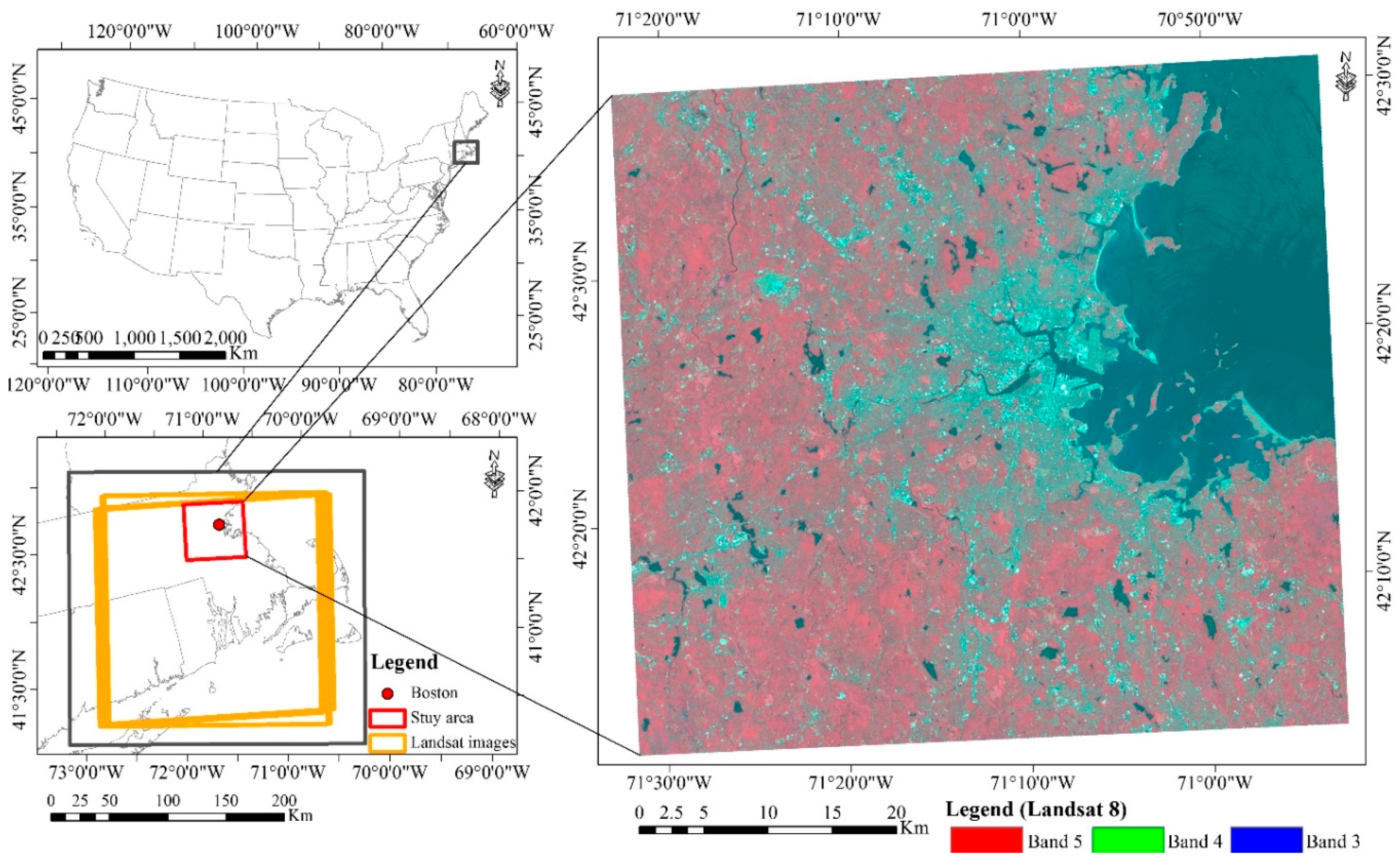
The study area covers one Landsat tile (12/31) in Boston, the capital city of Massachusetts, USA (Figure 1). As a historic municipal city, Boston hosts more than half million people living in an area of 233 km2 [36]. Boston is located on the east coast of the United States with its daily temperature in a range from −16.5 °C to 35.7 °C, having an average of 8.9 °C in spring, 21.7 °C in summer, 12.5 °C in autumn, and −0.13 °C in winter [37]. The large dynamics of temperature and greenness between summer and winter is optimal for studying the seasonality impacts on index-based impervious surface extraction.
2.2. Datasets
Three image sets, acquired from Landsat 5 Thematic Mapper (TM), Landsat 7 Enhanced Thematic Mapper Plus (ETM+), and Landsat 8 Operational Land Imager (OLI)-Thermal Infrared Sensor (TIRS), were collected in the study area. Four images for each sensor were downloaded to evaluate seasonal impacts on ISA mapping. Their acquisition dates, spectral bands and spatial resolutions are listed in Table 1. Atmospheric correction was performed to each image using the Atmospheric/Topographic Correction for Mountainous Terrain (ATCOR) software developed by German Aerospace Center, Wessling, Germany [38]. The Landsat images archived in the U.S. Geological Survey (USGS) data clearinghouse have been geo-rectified [39]. All images in Table 1 are geometrically matched to each other.
Training and validation samples were collected from the National Land Cover Database (NLCD) class maps on 2001 and 2011 downloaded from the USGS Data Clearinghouse. Only two classes were considered in this study, impervious surface (IS) and pervious surface (PS). In each NLCD class map, classes 22 (low intensity urban), 23 (medium intensity urban) and 24 (high intensity urban) were considered IS in this study. These NLCD classes represent land covers with 20–100% impervious surfaces [40]. All other classes were considered PS. In this way, a reference IS/PS layer was exported from the NLCD class map. The sampling points for each class were randomly selected using a stratified random sampling method. Sample points in 2001 were used for analysis of the 2001 Landsat ETM+ images, and those in 2011 were used for the 2010–2011 TM images and the 2015–2016 OLI-TIRS images. For each class, both training and validation sample sets contained 20% of the class pixels that were randomly selected in the reference layer.
3. Methodology
This study modified a current built-up index—the normalized difference impervious surface index (NDISI) developed by Xu [22]. By sharpening the TIR band assisted with reflective bands, the modified NDISI (MNDISI) was proposed. An automatic generalized Gaussian-based threshold selection method was then developed to identify the optimal threshold for segmenting IS from other land covers. To evaluate the performance of the MNDISI, its outputs were statistically compared with those from the original NDISI. The seasonal sensitivity of both indices in ISA mapping was further examined.
3.1. The Modified Normalized Difference Impervious Surface Index (MNDISI)
The NDISI is an effective method to enhance impervious surfaces and to suppress other land covers such as soil, sand, and water body. It is calculated as [22]:
where , , and are surface reflectance of green, near-infrared, and the first shortwave-infrared band, respectively. is the brightness temperature of the thermal band as calculated in Chander et al. [41]. The MNDWI is the modified normalized difference water index [42] to enhance water pixels with its calculation described in Equation (2). Both surface reflectance and in Equation (1) are stretched to [0, 255]. For Landsat OLI-TIRS, they are stretched to [0, 65,535] to maintain the 16-bit radiometric resolution.
For Landsat imagery, the pixel size of TIR band is much larger than 30 m of the reflective bands (as shown in Table 1). Here we apply the emissivity modulation theory to downscale the TIR image to 30 m pixel size. Land surface emissivity () varies with land covers on ground surfaces. In urban environments, vegetated surfaces have stronger thermal holding capacity and therefore, have higher cooling effects than non-vegetated areas. Sobrino et al. [43] measured the relationships between and green covers on a variety of ground surfaces. Linking to Landsat-extracted NDVI, at each 30 m pixel, it is calculated as [43]:
where is surface reflectance of the red band; is the proportion of vegetation in a pixel (also referred to as fractional vegetation cover) with its calculation described in Equation (4); and and represent the minimum and maximum NDVI values in an image, respectively. A pixel is considered bare soil when its NDVI value is less than, and full vegetation with its NDVI higher than . Pixels with NDVI values in between are a mixture of bare soil and vegetation. For Landsat images acquired in peak growing season (summer), Sobrino et al. [43] suggested , and . For those acquired in other seasons, is set 0.1–0.2, and is 0.4–0.5 for images in winter, spring and autumn, respectively.
Brightness temperature () in Equation (1) is extracted from a regular Landsat TIR band at coarser resolution. Contrarily, the in Equation (3) is extracted from the 30 m reflectance bands, and varies with green covers on ground. In this way, the emissivity-corrected land surface temperature () is sharpened to 30 m pixel size [44]:
where is the 30 m land surface temperatures in unit of K; is the central wavelength of the thermal band; and .
Using the sharpened in Equation (1), this study develops the modified NDISI (MNDISI) that is written as:
Similar to Equation (1), all input parameters in Equation (6) are stretched to [0, 255] for TM and ETM+ and [0, 65,535] for OLI-TIRS.
3.2. Automatic Threshold Selection of the MNDISI
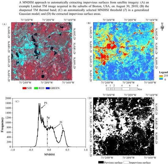
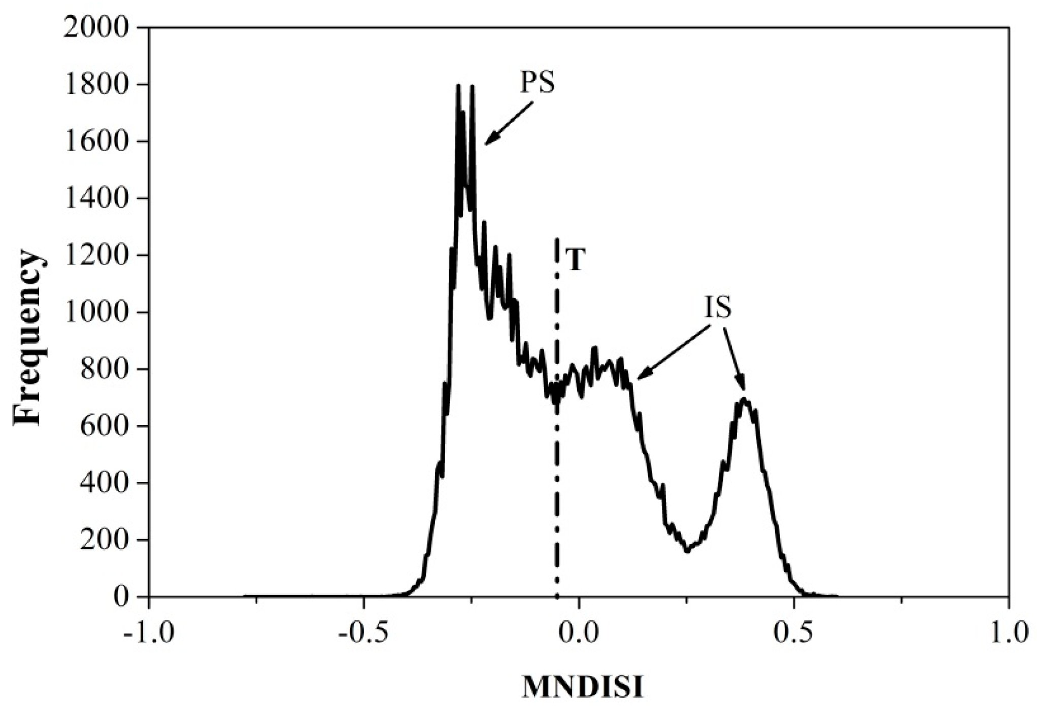
Impervious surfaces have higher MNDISI values than pervious surfaces. Figure 2 demonstrates an example MNDISI histogram derived from a TM image acquired on 30 August 2010, in which the IS pixels are located in the right side and PS pixels are in the left. The challenge of ISA mapping is thus to identify an optimal threshold in the MNDISI image. Manual selection of the threshold has been common in past index-based studies, which is time consuming, subjective and may highly affect the accuracies of ISA extraction.
Here, we propose an automatic threshold selection method based on the generalized Gaussian model [45,46]. Given a threshold value T (as marked in Figure 2), the generalized Gaussian optimization calculates the cost function (J) in the Kittler–Illingworth algorithm [47]:
where expresses the MNDISI histogram, with X varying from to , the minimum and maximum values of MNDISI incrementing at step l (l = 0.01 in this study). and are positive constants related to the shape parameters (and ) of the generalized Gaussian distribution for IS and PS pixels, respectively. The shape parameter determines the decay rate of the density function [48]. and denote the mean MNDISI of IS and PS pixels that are separated at T. and are a priori probabilities associated with IS and PS, respectively. is the entropy associated with the binary set of classes at T. For detailed information about the generalized Gaussian model, please see Bazi et al. [45].
The optimal threshold for segmenting IS and PS in the MNDISI histogram minimizes the cost function in Equation (7). Once is determined, it assigns all MNDISI pixels to IS (MNDISI > ) and PS (MNDISI < ), respectively. The ISA map is thus extracted.
3.3. Performance Evaluation
With an independent reference datasets from the NLCD products, accuracy assessment was conducted using the commonly applied error matrix approach [49,50]. The accuracy measures, i.e., overall accuracy (OA) and overall kappa coefficient (OK), were calculated.
To further evaluate the MNDISI performance, comparison analysis is conducted between the IS maps extracted from the MNDISI and the original NDISI. For each index, the spectral discrimination index (SDI) is calculated as [51,52]:
where and express the mean values of an index for IS and PS, respectively, and and are the standard deviations for the two classes.
The SDI reveals the degree of separation between IS and PS in aspects of their relative locations and spreads in the histograms [24]. A higher SDI indicates good separability. With the training data, the SDI values for both indices are compared to examine the effects of seasonality (spring, summer, autumn, and winter) and Landsat sensor types on ISA extraction.
4. Results and Analyses
4.1. The Sharpened TIR Imagery
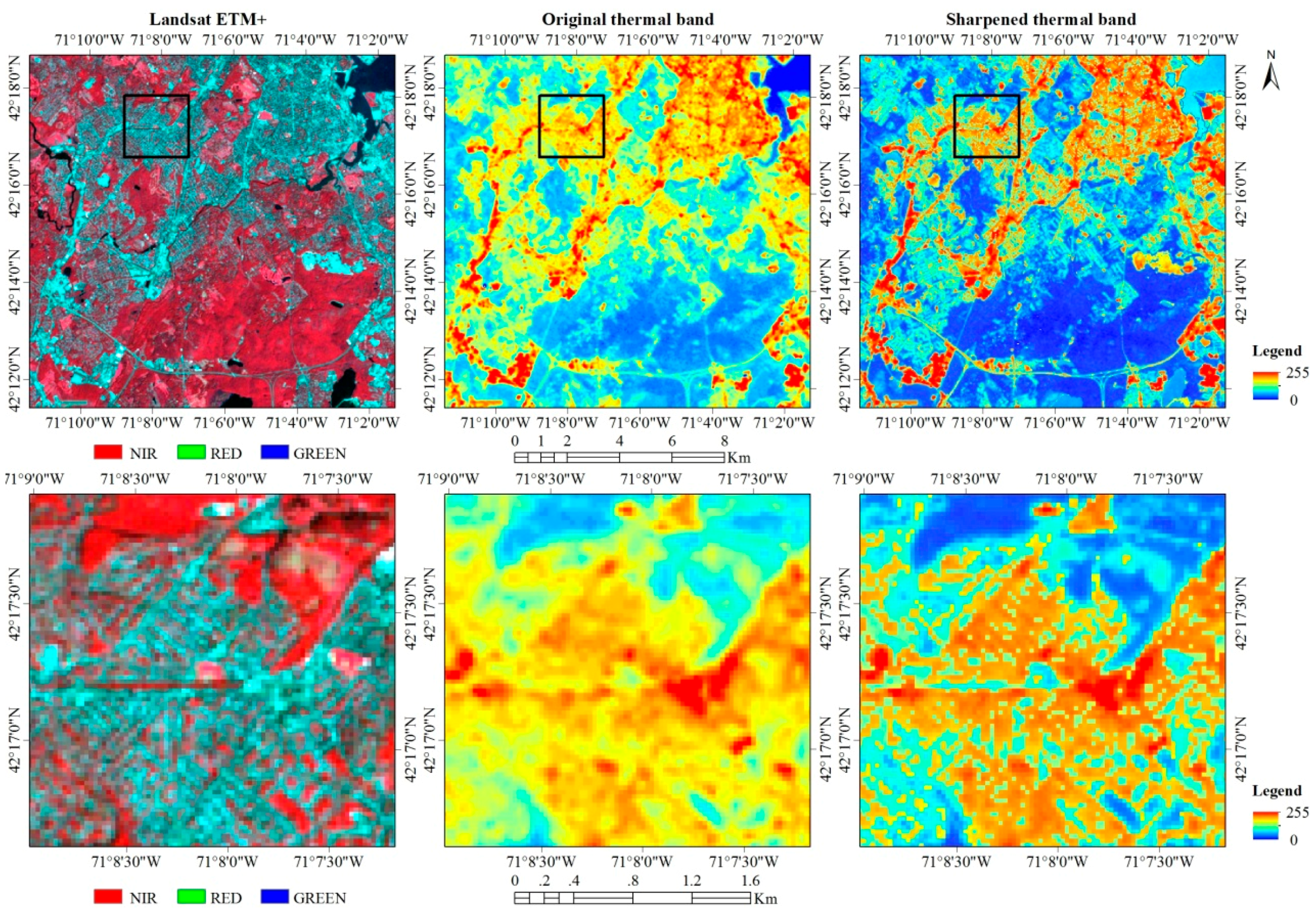
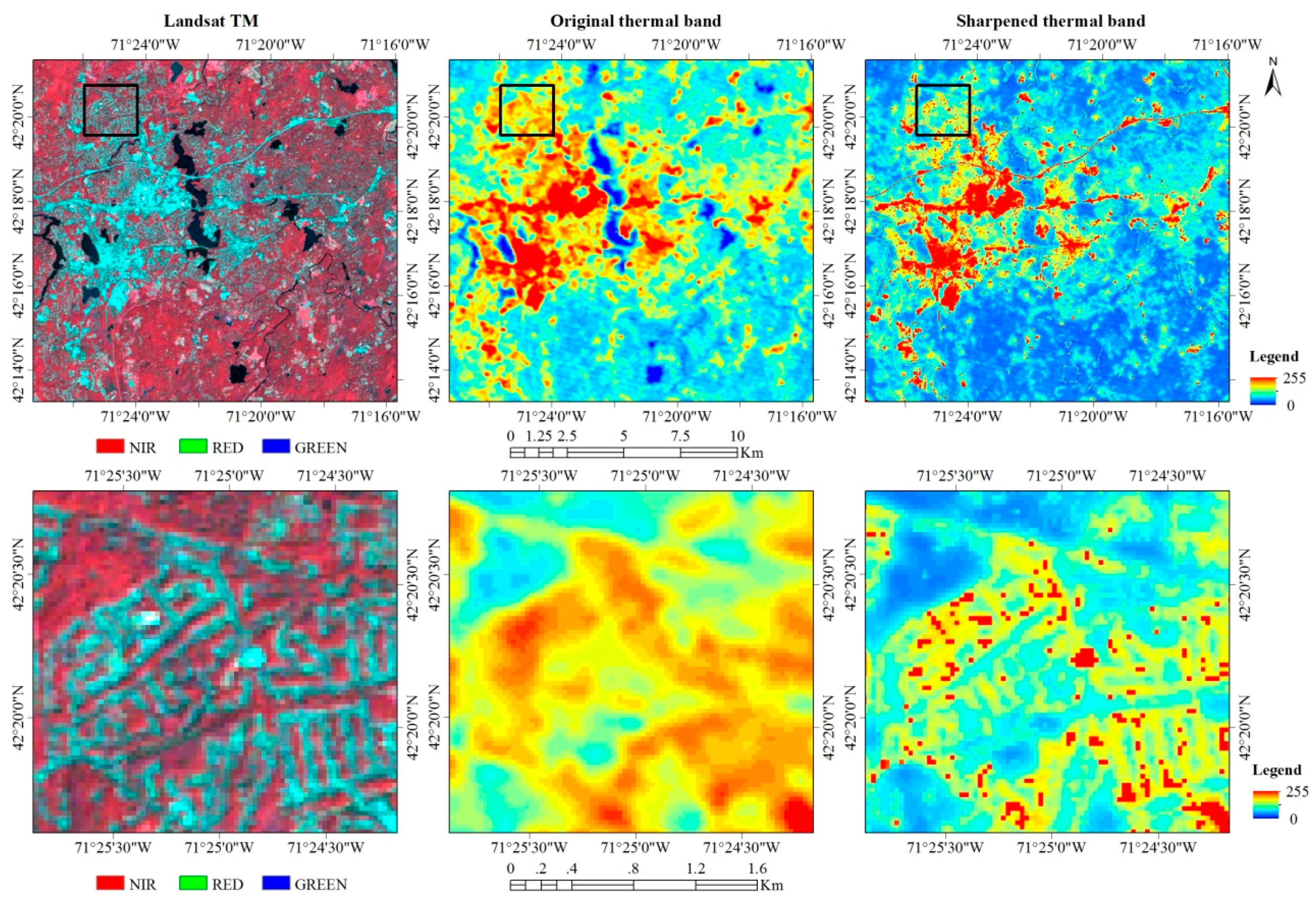
The sharpened 30-m thermal bands are displayed for summer images of ETM+ (Figure 3), TM (Figure 4) and OLI-TIRS (Figure 5). Images in other seasons (as listed in Table 1) were also processed and the ISA distributions were extracted. To better demonstration, in this section we only visually show the results from summer images. The seasonal variations of ISA mapping from all images in this study are described in Section 4.3 below.
The thermal images, including the original and sharpened TIR images, are stretched to [0, 255] for TM and ETM+ and [0, 65,535] for OLI-TIRS. The sharpened TIR images obviously show more details of urban information. Spatial variations in built-up areas are better revealed. The sharpened TIR image in Figure 3 is from the 60 m ETM+ band; that in Figure 4 is from the 120 m TM band; and that in Figure 4 is from the 100 m TIRS band. In original thermal bands, road network information is often lost, hot spots of dense urban cores are broader, and vegetated residential areas have higher values due to mixed-pixel problems. All these problems lead to IS overestimation. The sharpened thermal band, on the other hand, better identifies urban areas and road networks for improved ISA mapping.
4.2. Automatic Threshold Selection for ISA Mapping
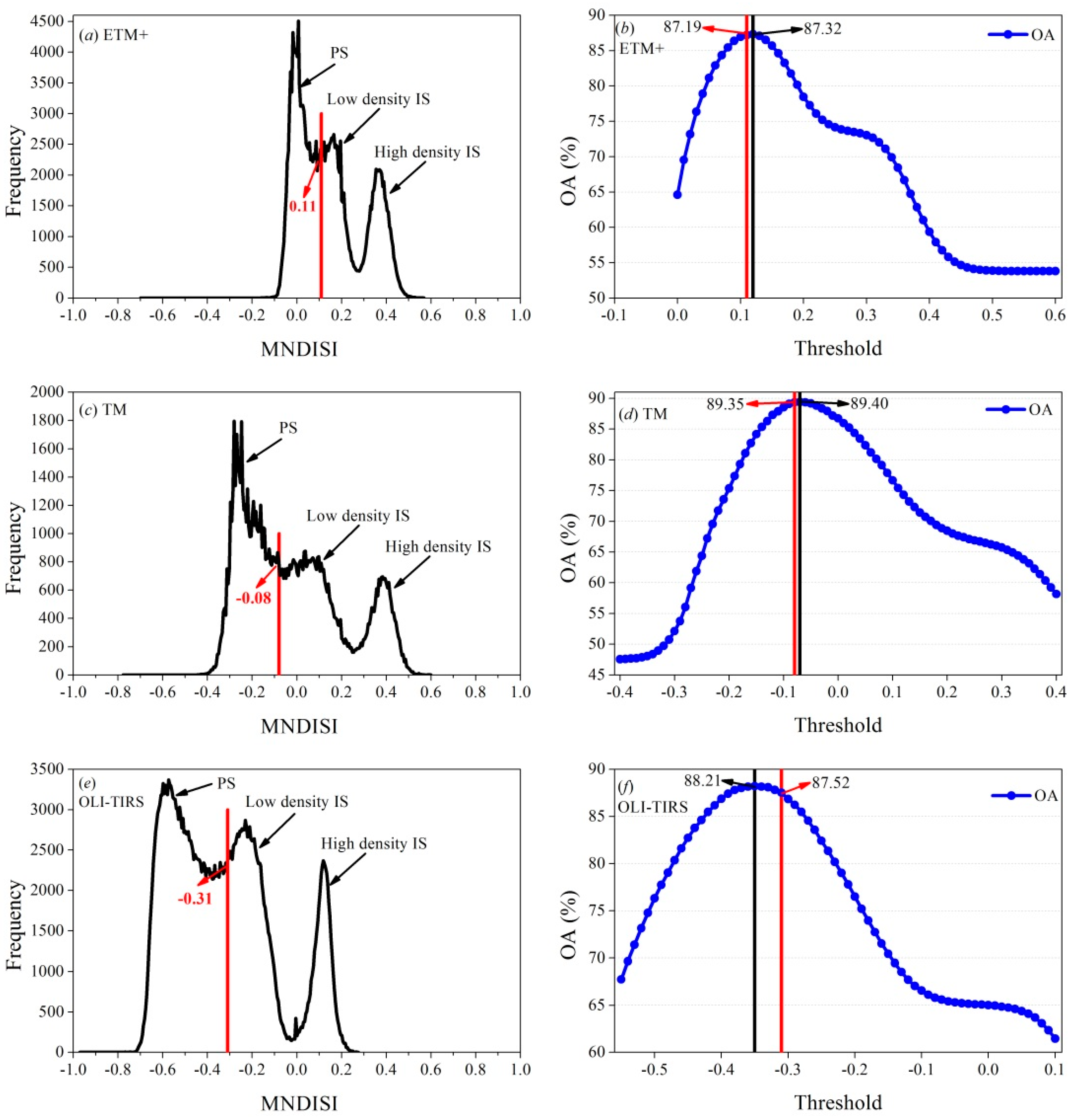
With training samples for each image, one optimal threshold was identified to split all MNDISI pixels into IS and PS. Using three summer images as examples, Figure 6 shows the process of automatic threshold selection and its optimization effects for ETM+ (Figure 6a), TM (Figure 6c) and OLI (Figure 6e) sensors. The three peaks in all histograms represent high density IS pixels in the far right, low-density IS in the middle, and PS (all other land covers) in the left. The optimal thresholds, determined from the proposed automatic threshold selection, are −0.08, 0.11 and −0.31 (as marked in the red lines), respectively.
Performance of these automatically selected thresholds was evaluated by comparing with randomly selected thresholds. At any given threshold, The IS and PS were segmented from the MNDISI image and the overall accuracy (OA) of the segmentation was calculated using the validation samples. For each image, an OA curve is traced with the threshold iteratively changing at a step of 0.01 (Figure 6b,d,f). For all three images, the automatically selected thresholds (marked in red line) are close to the one with the highest OA value (marked in black line) in all OA curves (Figure 6b,d,f). Because of the higher radiometric resolution of the OLI image, the OA difference between the automatic threshold and the peak threshold seems larger than those of TM and ETM+. Figure 6 indicates that our proposed automatic threshold selection is an effective method to identify the optimal threshold for ISA mapping.
4.3. Performance Evaluation
Comparison analysis was performed between the proposed MNDISI and the original NDISI using Landsat images from three sensors in four seasons. Automatic threshold selection was employed for both indices. The comparison included seasonality analysis, visual comparison, statistical measures, and accuracy assessment between the two indices.
4.3.1. Seasonality Analysis for ISA Mapping
The separability measures (SDI) of both indices from the three sensors and four seasons are plotted in Figure 7. Generally, IS and PS have higher separability for the MNDISI than the NDISI among all three sensor types: TM (Figure 7a), ETM+ (Figure 7b), and OLI-TIRS (Figure 7c). Seasonal trends of the SDI for the two indices are similar, all having best performance (SDI > 1.0) in summer when vegetation is in peak growth. In spring and autumn, green vegetation is less vigorous and is often exposed with bare soil. Spectral similarity between IS and PS therefore results in lower SDI values in these seasons. Limited greenness and occasional snow disturbance in winter attribute to the lowest SDI values in this season. For all three images in winter, the MNDISI has improved separability compared to NDISI, increasing from around 0.1–0.2 to 0.4–0.5. The relatively low SDI values, however, indicate that winter images cannot be effectively employed to extract impervious surfaces.
In short, Figure 7 suggests that summer imagery was optimal for ISA mapping from both indices. The comparison analyses in the following sections were only performed using the summer images.
4.3.2. Visual Comparison
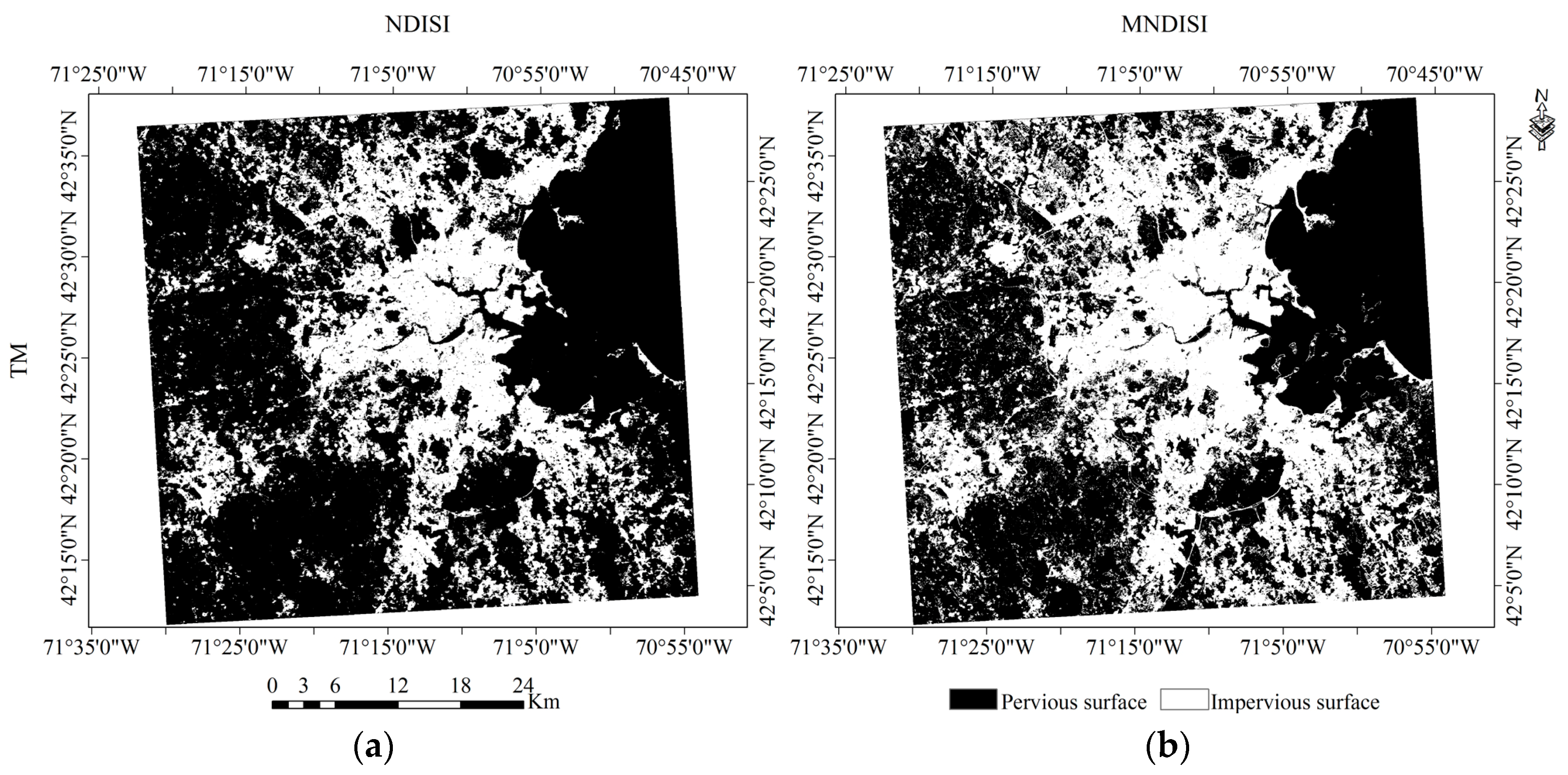
Figure 8 demonstrates the visual differences of the extracted ISA distributions from the two indices of the TM summer image. Overall, the ISA distributions from both indices are similarly high in urban lands. In areas out of the urban core, the NDISI-extracted IS areas (Figure 8a) have fewer details than those from the MNDISI (Figure 8b), resulting in the loss of small-size impervious surface in these areas. In other words, the MNDISI reduces the omission errors in areas with lower urban densities.
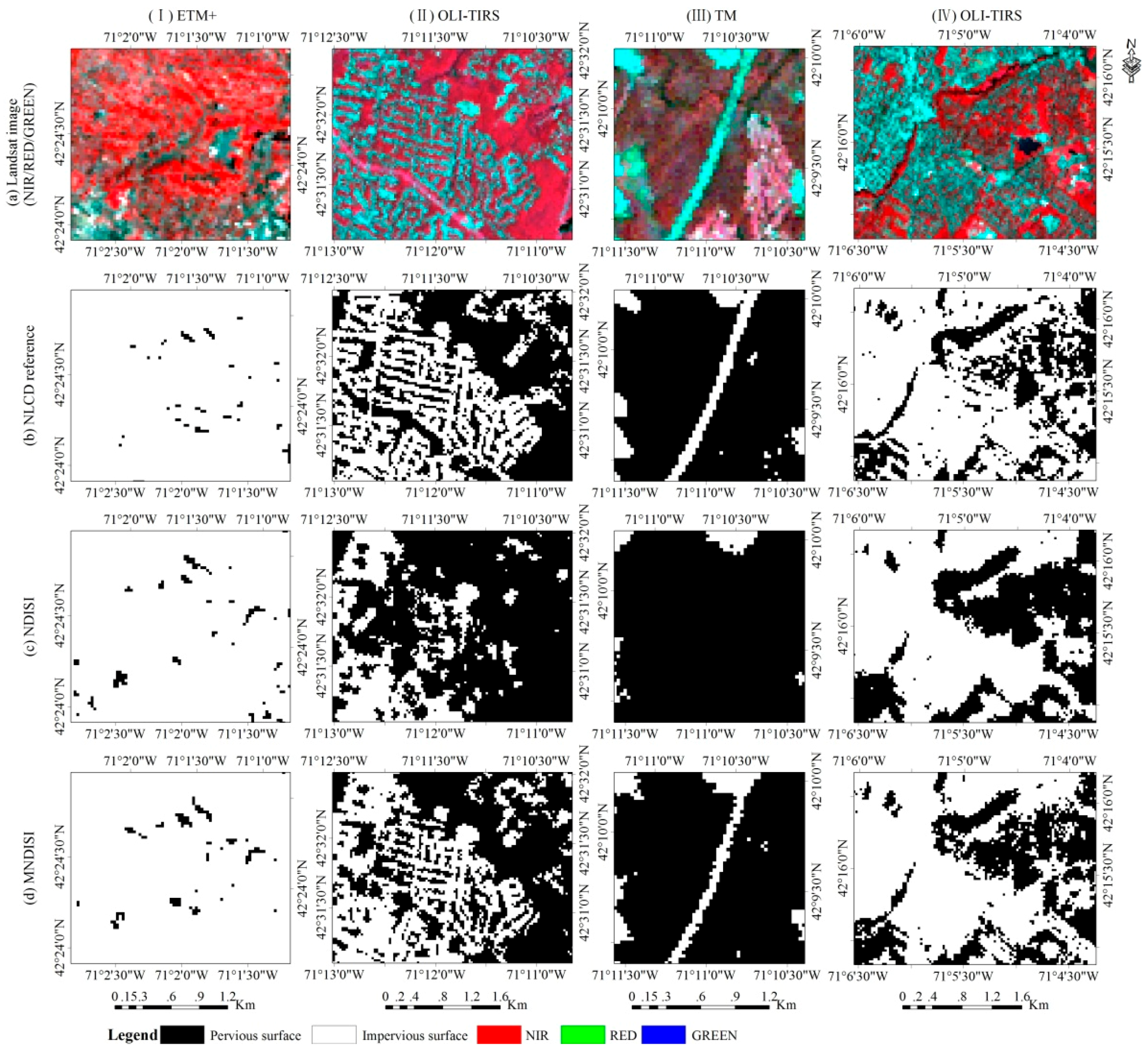
To better demonstrate the effectiveness of our proposed MNDISI, subsets with representative urban features are selected to compare the effectiveness of the two indices with summer images (Figure 9): central business district (CBD), residential area, road infrastructure, and suburban–rural area. One Landsat image type is used in a subset. In the CBD area (Figure 9I-a), one can observe that vegetation and impervious surfaces are often mixed. In the NLCD-extracted IS reference layer (Figure 9I-b), almost all pixels are classified as IS except a few vegetative clusters. Given the 60 m resolution of the ETM+ thermal band, both the NDISI (Figure 9I-c) and the MNDISI (Figure 9I-d) generate better ISA results than the NLCD reference. In residential areas (Figure 9II-a), neighborhood streets and building clusters are clear. The NLCD reference layer still overestimates the IS class (Figure 9II-b). The NDISI can only obtain agglomerated urban clusters (Figure 9II-c). Due to the low resolution (100 m) of the OLI-TIRS thermal band, street network information is lost. With sharpened thermal image, the MNDISI fairly extracts both the agglomerated IS clusters and detailed road network in the neighborhood (Figure 9II-d). Road infrastructures such as highways are a significant component of urban impervious surfaces (Figure 9III-a). The linear feature is easily classified in the NLCD product (Figure 9III-b). The NDISI is unable to extract road information because of the low resolution (120 m) of the TM thermal band. With sharpened thermal image, the MNDISI fairly extracts the highway that is lost in the NDISI-extracted map. In suburban–rural areas, bare surfaces are observed in areas such as newly cleared construction fields and fallow agricultural lands (Figure 9IV-a). Bare fields are often confused with impervious surfaces in Landsat imagery due to their similar spectral characteristics, resulting in noisy, salt-and-pepper appearances in the NLCD reference map (Figure 9IV-b). The IS is better delineated from bare soil in the NDISI (Figure 9IV-c) and MNDISI (Figure 9IV-d) indices. Similarly, the MNDISI results in more detailed IS distributions than the NDISI.
4.3.3. Statistical Comparison
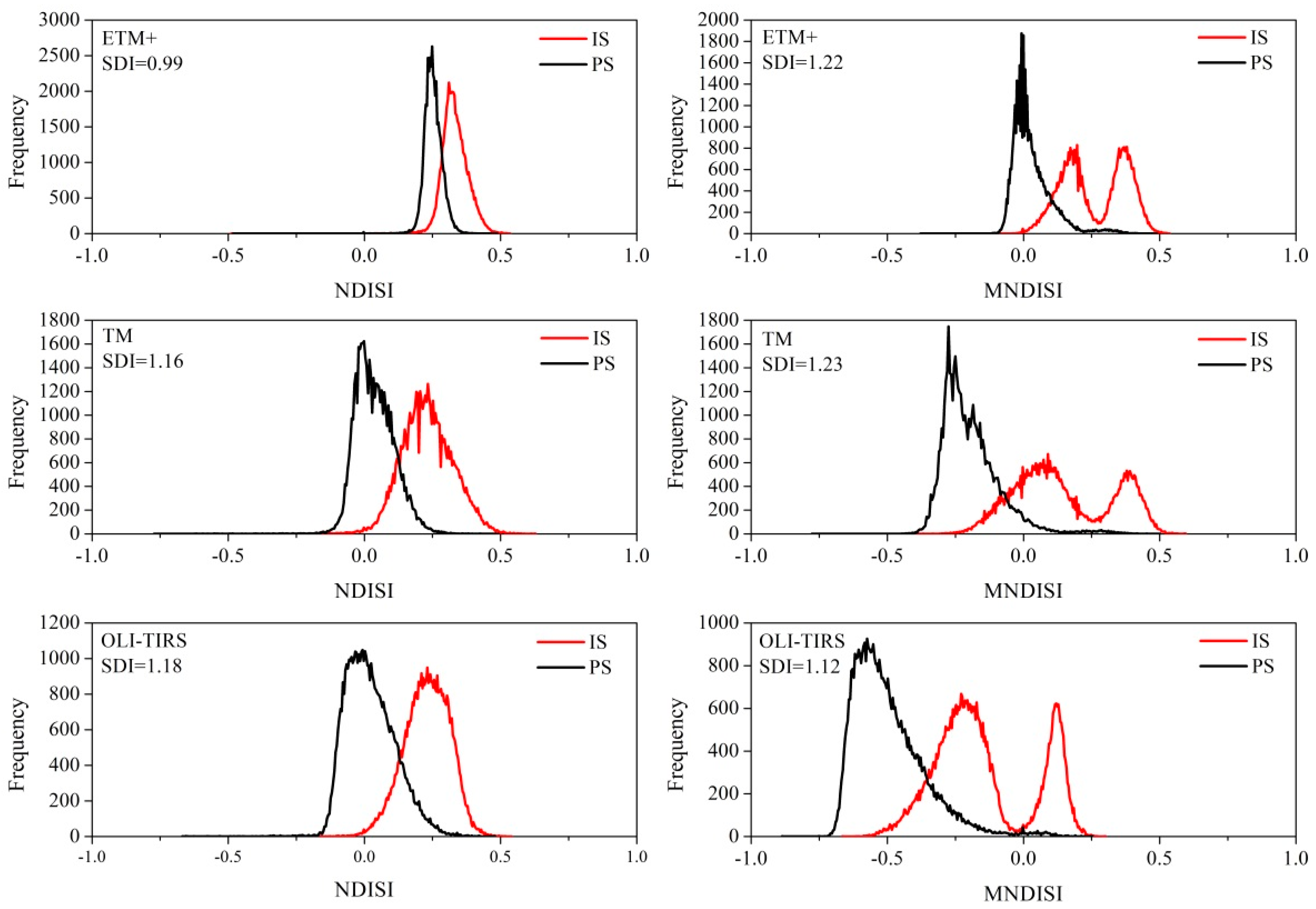
Figure 10 compares the histograms of IS and PS for the NDISI and MNDISI images from the three sensors. Visually, the two classes can be delineated, although there is a large portion of overlay. More specifically, the histograms of IS derived from the MNDISI have two crests corresponding to low density IS and high density IS, respectively. Therefore, the MNDISI can completely identify high density IS pixels, and improve the separability between low density IS and PS pixels. In addition, for both classes, the MNDISI has wider data ranges than the NDISI, which also indicates the MNDISI’s improved performance for separating impervious surface from other land covers. All SDI values are around 1.0 and above, indicating good separability between IS and PS classes from both built-up indices. For the same Landsat image, the SDI value of MNDISI-derived maps is higher than that of NDISI, although the SDI values from the OLI-TIRS are similar. All aspects above reveal that our proposed MNDISI has higher capability of extracting impervious surfaces from Landsat imagery.
4.3.4. Accuracy Assessment
With validation samples, the two accuracy measures (OA and OK) are compared between the ISA outputs of the two indices with summer images from the three Landsat sensors (Table 2). For each index, the OA and OK derived from the three images are similar. The MNDISI improves the ISA extraction with higher accuracies. For the three sensors, the ETM+ image has the lowest increase of accuracies, followed by OLI-TIRS then TM. Coincidently, this sequence agrees with the spatial resolutions of their thermal bands, i.e., 60, 100 and 120 m, respectively. It should be noted, however, the improvements among these three sensors are not significantly large, which also confirms that Landsat imagery from the three sensors has similar performance in ISA mapping.
5. Discussion
This study aims to extract impervious surfaces from the built-up index with improved thermal integration and automatic threshold selection. Several innovative experiments are carried out. Compared with the original NDISI, our proposed MNDISI takes advantage of sharpened Landsat thermal channels based on emissivity modulation theories. Using reflective bands to refine emissivity that varies with green covers, it enhances the identification of heterogeneous urban land covers, especially in low impervious surface areas. As shown in the histograms of impervious surfaces and pervious surfaces in Figure 10, the distributions of low-density IS pixels are overlaid with PS pixels. The MNDISI maximally stretches the high-density and low-density IS classes and is thus superior for ISA mapping. Furthermore, subjective threshold selection has been considered a key problem in index-based ISA mapping [25]. In this study, a generalized Gaussian-based automatic threshold selection method is proposed to automatically identify the optimal threshold to segment impervious surfaces from other land covers in the MNDISI image. Automation of this process reduces the uncertainties from the subjective manual selection of thresholds that vary from scene to scene. The reduced time and labor cost also makes it more feasible for regional and even global ISA mapping with Landsat imagery.
This study contributes to the literature of ISA mapping with its comprehensive comparison analysis among different image sources (three Landsat sensors) and seasonality (four seasons), which has not been explicitly documented in past studies. The findings of this study suggest that satellite images acquired in summer are most suitable for ISA mapping, and those from all three Landsat sensors (TM/ETM+/OLI-TIRS) are good image sources. Although Landsat data collection is limited by its 16-day revisit cycle, and image quality is frequently contaminated by cloud cover, it is more reliable to collect optimal images in growing seasons from all Landsat sensors. In this sense, ISA mapping at regional even global scales also becomes practically feasible.
While built-up indices have been considered promising for large-area ISA mapping from optical satellite imagery at local, national, regional and global scales, our results indicate that there still exists limitations and challenges for index-based extraction of impervious surfaces. Firstly, the mixed-pixel problem remains a major challenge for ISA mapping using medium resolution Landsat imagery. Secondly, spectral similarity between different urban land covers always raises uncertainties in heterogeneous urban environments. For example, past studies have shown that bare soil can be easily confused with impervious surfaces [14]. In the histograms (Figure 10) of this study, the overlaid areas between IS and PS clearly demonstrate the confusion between the brighter PS pixels (such as bare soil) and darker IS pixels (such as low-density urban). Although the MNDISI improved the separation by enhancing the IS values, the overlay remains unsolved. Further investigation is needed to tackle the problem of spectral similarity of urban land covers, especially impervious surfaces and bare soil. More recently, several indices specifically dealing with bare soil surfaces have been published [53,54,55]. These bare soil indices could be coupled with built-up indices for improved ISA mapping. Finally, thermal image is utilized in our proposed MNDISI. However, the TIR band is not always available in the same image acquired from one sensor (e.g., Landsat Multispectral Scanner (MSS)). The feasibility of fusing thermal and reflective bands from different sensors will be tested in the future.
Other remote sensing categories have also been examined in mapping urban environments. For example, Synthetic Aperture Radar (SAR) imagery is found promising due to its all-weather conditions and strong double bounce scattering of urban features [56,57,58]. In the future work, with the emergence of advanced satellite systems, index-based urban mapping with automatic threshold section could be a promising solution for rapidly and automatically mapping of ISA distribution at a regional and global scale.
6. Conclusions
This study proposes an improved impervious surface index, the MNDISI, by integrating the sharpened thermal band to reflective bands of Landsat imagery. An automatic threshold selection method is developed to optimally segment impervious surfaces from other land covers in the MNDISI image. Several findings are drawn:
- (1)
- Our results show that built-up indices are sensitive to seasonal changes in urban environments; and imagery acquired in summer is the best for ISA mapping. The three Landsat sensors, TM, ETM+ and OLITIRS, do not have significant differences in extracting impervious surfaces.
- (2)
- By downscaling thermal information using green cover-related emissivity, the proposed MNDISI enhances urban features especially, for low density impervious surfaces. The OA and OK values derived from Landsat imagery of all three sensors are higher than 87% and 74%, respectively.
- (3)
- With the rich set of Landsat imagery from its multiple sensors in the past 40 years, the proposed MNDISI together with automatic threshold selection approach could become an efficient tool for rapid mapping of impervious surfaces at regional and global scales, and therefore provides vital information to study broad impacts of human activities across the globe.
Acknowledgments
The research in this paper was supported by National Key Research and Development Program (Grant No. 2016YFA0600302), the International Partnership Program of Chinese Academy of Sciences (Grant No. 131C11KYSB20160061), the National Natural Science Foundation of China (Grant No. 41201357), “One-Three-Five” Strategic Planning by the Institute of Remote Sensing and Digital Earth, CAS (Grant No. Y4SG0500CX), and Key Laboratory of Satellite Mapping Technology and Application, National Administration of Surveying, Mapping and Geoinformation (Grant No. KLMSTA-201605).
Author Contributions
Zhongchang Sun contributed the main idea, designed the study method, and drafted the manuscript. Cuizhen Wang overviewed the process and completed the manuscript. Huadong Guo supervised the framework. Ranran Shang performed the Landsat image analysis. The manuscript was improved with contributions from all co-authors.
Conflicts of Interest
The authors declare no conflict of interest.
References
- Weng, Q.H. Remote sensing of impervious surfaces in the urban areas: Requirements, methods, and trends. Remote Sens. Environ. 2012, 117, 34–49. [Google Scholar] [CrossRef]
- Sun, Z.C.; Li, X.W.; Fu, W.X.; Li, Y.K.; Tang, D.S. Long-term effects of land use/land cover change on surface runoff in urban areas of Beijing, China. J. Appl. Remote Sens. 2014, 8, 084596. [Google Scholar] [CrossRef]
- Mathew, A.; Khandelwal, S.; Kaul, N. Spatial and temporal variations of urban heat island effect and the effect of percentage impervious surface area and elevation on land surface temperature: Study of Chandigarh city, India. Sustain. Cities Soc. 2016, 26, 264–277. [Google Scholar] [CrossRef]
- Melesse, A.M.; Weng, Q.; Thenkabail, P.S.; Senay, G.B. Remote sensing sensors and applications in environmental resources mapping and modelling. Sensors 2007, 7, 3209–3241. [Google Scholar] [CrossRef]
- Liu, Z.H.; Wang, Y.L.; Li, Z.G.; Peng, J. Impervious surface impact on water quality in the process of rapid urbanization in Shenzhen, China. Environ. Earth Sci. 2013, 68, 2365–2373. [Google Scholar] [CrossRef]
- Kim, H.; Jeong, H.; Jeon, J.; Bae, S. The impact of impervious surface on water quality and its threshold in Korea. Water 2016, 8, 111. [Google Scholar] [CrossRef]
- Touchaei, A.G.; Akbari, H.; Tessum, C.W. Effect of increasing urban albedo on meteorology and air quality of Montreal (Canada)—Episodic simulation of heat wave in 2005. Atmos. Environ. 2016, 132, 188–206. [Google Scholar] [CrossRef]
- Schneider, A.; Friedl, M.A.; Potere, D. A new map of global urban extent from MODIS satellite data. Environ. Res. Lett. 2009, 4, 044003. [Google Scholar] [CrossRef]
- Seto, K.C.; Fragkias, M.; Güneralp, B.; Reilly, M.K. A meta-analysis of global urban land expansion. PLoS ONE 2011, 6, e23777. [Google Scholar] [CrossRef] [PubMed]
- Sexton, J.O.; Song, X.P.; Huang, C.Q.; Channan, S.; Baker, M.E.; Townshend, J.R.G. Urban growth of the Washington, D.C.–Baltimore, MD metropolitan region from 1984 to 2010 by annual, Landsat-based estimates of impervious cover. Remote Sens. Environ. 2013, 129, 42–53. [Google Scholar] [CrossRef]
- Zhang, L.; Weng, Q.H. Annual dynamics of impervious surface in the Pearl River Delta, China, from 1988 to 2013, using time series Landsat imagery. ISPRS J. Photogramm. 2016, 113, 86–96. [Google Scholar] [CrossRef]
- Song, X.P.; Sexton, J.O.; Huang, C.Q.; Channan, S.; Townshend, J.R.G. Characterizing the magnitude, timing and duration of urban growth from time series of Landsat-based estimates of impervious cover. Remote Sens. Environ. 2016, 175, 1–13. [Google Scholar] [CrossRef]
- Yu, S.S.; Sun, Z.C.; Guo, H.D.; Zhao, X.W.; Sun, L.; Wu, M.F. Monitoring and analyzing the spatial dynamics and patterns of megacities along the Maritime Silk Road. J. Remote Sens. 2017, 21, 1993–2002. [Google Scholar] [CrossRef]
- Sun, Z.C.; Guo, H.D.; Li, X.W.; Lu, L.L. Estimating urban impervious surfaces from Landsat-5 TM imagery using multilayer perceptron neural network and support vector machine. J. Appl. Remote Sens. 2011, 5, 053501. [Google Scholar] [CrossRef]
- Taubenböck, H.; Esch, T.; Felbier, A.; Wiesner, M.; Roth, A.; Dech, S. Monitoring urbanization in mega cities from space. Remote Sens. Environ. 2012, 117, 162–176. [Google Scholar] [CrossRef]
- Franke, J.; Roberts, D.A.; Halligan, K.; Menz, G. Hierarchical multiple endmember spectral mixture analysis (MESMA) of hyperspectral imagery for urban environments. Remote Sens. Environ. 2009, 113, 1712–1723. [Google Scholar] [CrossRef]
- Deng, C.B.; Wu, C.S. A spatially adaptive spectral mixture analysis for mapping subpixel urban impervious surface distribution. Remote Sens. Environ. 2013, 133, 62–70. [Google Scholar] [CrossRef]
- Bauer, M.E.; Loffelholz, B.C.; Willson, B. Estimating and mapping impervious surface area by regression analysis of Landsat imagery. In Remote Sensing of Impervious Surfaces; Weng, Q.H., Ed.; Taylor & Francis Group, LLC: Boca Raton, FL, USA, 2008; pp. 3–19. [Google Scholar]
- Im, J.; Lu, Z.Y.; Rhee, J.; Quackenbush, L.J. Impervious surface quantification using a synthesis of artificial immune networks and decision/regression trees from multi-sensor data. Remote Sens. Environ. 2012, 117, 102–113. [Google Scholar] [CrossRef]
- Yang, L.M.; Huang, C.Q.; Homer, C.G.; Wylie, B.K.; Coan, M.J. An approach for mapping large-area impervious surfaces: Synergistic use of Landsat 7 ETM+ and high spatial resolution imagery. Can. J. Remote Sens. 2003, 29, 230–240. [Google Scholar] [CrossRef]
- Lu, D.S.; Moran, E.; Hetrick, S. Detection impervious surface change with multitemporal Landsat images in an urban-rural frontier. ISPRS J. Photogramm. Remote Sens. 2011, 66, 298–306. [Google Scholar] [CrossRef] [PubMed]
- Xu, H. Analysis of impervious surface and its impact on urban heat environment using the normalized difference impervious surface index (NDISI). Photogramm. Eng. Remote Sens. 2010, 76, 557–565. [Google Scholar] [CrossRef]
- Sun, G.Y.; Chen, X.L.; Jia, X.P.; Yao, Y.J.; Wang, Z.J. Combinational build-up index (CBI) for effective impervious surface mapping in urban areas. IEEE J. Sel. Top. Appl. Earth Obs. Remote Sens. 2016, 9, 2081–2092. [Google Scholar] [CrossRef]
- Deng, C.B.; Wu, C.S. BCI: A biophysical composition index for remote sensing of urban environments. Remote Sens. Environ. 2012, 127, 247–259. [Google Scholar] [CrossRef]
- Lu, D.S.; Li, G.Y.; Kuang, W.H.; Moran, E. Methods to extract impervious surface areas from satellite images. Int. J. Digit. Earth 2014, 7, 93–112. [Google Scholar] [CrossRef]
- Xu, H.Q.; Wang, M.Y. Remote sensing-based retrieval of ground impervious surfaces. J. Remote Sens. 2016, 20, 1270–1289. [Google Scholar] [CrossRef]
- Kawamura, M.; Jayamana, S.; Tsujiko, Y. Relation between social and environmental conditions in Colombo Sri Lanka and the urban index estimated by satellite remote sensing data. Int. Arch. Photogramm. Remote Sens. 1996, 31, 321–326. [Google Scholar]
- Carlson, T.N.; Arthur, S.T. The impact of land use-land cover changes due to urbanization on surface microclimate and hydrology: A satellite perspective. Glob. Planet. Chang. 2000, 25, 49–65. [Google Scholar] [CrossRef]
- Zha, Y.; Gao, Y.; Ni, S. Use of normalized difference built-up index in automatically mapping urban areas from TM imagery. Int. J. Remote Sens. 2003, 24, 583–594. [Google Scholar] [CrossRef]
- Xu, H.Q. A new index for delineating built-up land features in satellite imagery. Int. J. Remote Sens. 2008, 29, 4269–4276. [Google Scholar] [CrossRef]
- Ma, Y.; Kuang, Y.Q.; Huang, N.S. Coupling urbanization analyses for studying urban thermal environment and its interplay with biophysical parameters based on TM/ETM+ imagery. Int. J. Appl. Earth Obs. 2010, 12, 110–118. [Google Scholar] [CrossRef]
- As-Syakur, A.R.; Adnyana, I.; Arthana, I.W.; Nuarsa, I.W. Enhanced built-up and bareness index (EBBI) for mapping built-up and bare land in an urban area. Remote Sens. 2012, 4, 2957–2970. [Google Scholar] [CrossRef]
- Liu, C.; Shao, Z.F.; Chen, M.; Luo, H. MNDISI: A multisource composition index for impervious surface area estimation at the individual city scale. Remote Sens. Lett. 2013, 4, 803–812. [Google Scholar] [CrossRef]
- Zhou, Y.; Yang, G.; Wang, S.X.; Wang, L.T.; Wang, F.T.; Liu, X.F. A new index for mapping built-up and bare land areas from Landsat-8 OLI data. Remote Sens. Lett. 2014, 5, 862–871. [Google Scholar] [CrossRef]
- Wang, Z.Q.; Gang, C.C.; Li, X.L.; Chen, Y.Z.; Li, J.L. Application of a normalized difference impervious index (NDII) to extract urban impervious surface features based on Landsat TM images. Int. J. Remote Sens. 2015, 36, 1055–1069. [Google Scholar] [CrossRef]
- United States Census Bureau. Population and Housing Occupancy Status: 2010-State-County Subdivision, 2010-State-County Subdivision, 2010 Census Redistricting Data (Public Law 94-171) Summary File. Available online: https://www.census.gov/prod/cen2010/doc/pl94-171.pdf (accessed on 15 February 2017).
- National Oceanic and Atmospheric Administration (NOAA). Now Data—NOAA Online Weather Data. Available online: http://w2.weather.gov/climate/xmacis.php?wfo=box (accessed on 15 February 2017).
- Richter, R.; Schläpfer, D. Atmospheric/Topographic Correction for Satellite Imagery: ATCOR-2/3 User Guide, DLR-IB 565-01/15; German Aerospace Center: Wessling, Germany, 2015. [Google Scholar]
- U.S. Geological Survey (USGS). Landsat 8 (L8) Data Users Handbook. Available online: https://landsat.usgs.gov/landsat-8-l8-data-users-handbook (accessed on 10 February 2017).
- Homer, C.G.; Dewitz, J.A.; Yang, L.; Jin, S.; Danielson, P.; Xian, G.; Coulston, J.; Herold, N.D.; Wickham, J.D.; Megown, K. Completion of the 2011 National Land Cover Database for the conterminous United States-Representing a decade of land cover change information. Photogramm. Eng. Remote Sens. 2015, 81, 345–354. [Google Scholar] [CrossRef]
- Chander, G.; Markham, B.L.; Helder, D.L. Summary of current radiometric calibration coefficients for Landsat MSS, TM, ETM+, and EO-1 ALI sensors. Remote Sens. Environ. 2009, 113, 893–903. [Google Scholar] [CrossRef]
- Xu, H.Q. Modification of normalized difference water index (NDWI) to enhance open water features in remotely sensed imagery. Int. J. Remote Sens. 2006, 27, 3025–3033. [Google Scholar] [CrossRef]
- Sobrino, J.A.; Jiménez-Muñoz, J.C.; Sòria, G.; Romaguera, M.; Guanter, L.; Moreno, J.; Plaza, A.; Martínez, P. Land surface emissivity retrieval from different VNIR and TIR sensors. IEEE Trans. Geosci. Remote Sens. 2008, 46, 316–327. [Google Scholar] [CrossRef]
- Weng, Q.H.; Lu, D.S.; Schubring, J. Estimation of land surface temperature–vegetation abundance relationship for urban heat island studies. Remote Sens. Environ. 2004, 89, 467–483. [Google Scholar] [CrossRef]
- Bazi, Y.; Bruzzone, L.; Melgani, F. An Unsupervised Approach Based on the Generalized Gaussian Model to Automatic Change Detection in Multitemporal SAR Images. IEEE Trans. Geosci. Remote Sens. 2005, 43, 874–887. [Google Scholar] [CrossRef]
- Li, X.W.; Zhang, L.; Guo, H.D.; Sun, Z.C.; Liang, L. New approaches to urban area change detection using multitemporal RADARSAT-2 polarimetric synthetic aperture radar (SAR) data. Can. J. Remote Sens. 2012, 38, 253–266. [Google Scholar] [CrossRef]
- Kittler, J.; Illingworth, J. Minimum error thresholding. Pattern Recognit. 1986, 19, 41–47. [Google Scholar] [CrossRef]
- Sharifi, K.; Leon-Garcia, A. Estimation of shape parameter for generalized Gaussian distributions in subband decomposition of video. IEEE Trans. Circuits Syst. Video Technol. 1995, 5, 52–56. [Google Scholar] [CrossRef]
- Congalton, R.G. A review of assessing the accuracy of classifications of remotely sensed data. Remote Sens. Environ. 1991, 37, 35–46. [Google Scholar] [CrossRef]
- Foody, G.M. Status of land cover classification accuracy assessment. Remote Sens. Environ. 2002, 80, 185–201. [Google Scholar] [CrossRef]
- Kaufman, Y.J.; Remer, L.A. Detection of forests using mid-IR reflectance: An application for aerosol studies. IEEE Trans. Geosci. Remote Sens. 1994, 32, 672–683. [Google Scholar] [CrossRef]
- Pereira, J.M. A comparative evaluation of NOAA/AVHRR vegetation indexes for burned surface detection and mapping. IEEE Trans. Geosci. Remote Sens. 1999, 37, 217–226. [Google Scholar] [CrossRef]
- Deng, Y.B.; Wu, C.S.; Li, M.; Chen, R.R. RNDSI: A ratio normalized difference soil index for remote sensing of urban/suburban environments. Int. J. Appl. Earth Obs. Geoinf. 2015, 39, 40–48. [Google Scholar] [CrossRef]
- Li, H.; Wang, C.; Zhong, C.; Su, A.; Xiong, C.; Wang, J.; Liu, J. Mapping urban bare land automatically from Landsat imagery with a simple index. Remote Sens. 2017, 9, 249. [Google Scholar] [CrossRef]
- Piyoosh, A.K.; Ghosh, S.K. Development of a modified bare soil and urban index for Landsat 8 satellite data. Geocarto Int. 2017, 1, 1–20. [Google Scholar] [CrossRef]
- Guo, H.D.; Yang, H.N.; Sun, Z.C.; Li, X.W.; Wang, C.Z. Synergistic Use of Optical and PolSAR Imagery for Urban Impervious Surface Estimation. Photogramm. Eng. Remote Sens. 2014, 80, 91–102. [Google Scholar] [CrossRef]
- Esch, T.; Marconcini, M.; Felbier, A.; Heldens, W.; Huber, M.; Schwinger, M.; Taubenböck, H.; Müller, A.; Dech, S. Urban footprint processor—Fully automated processing chain generating settlement masks from global data of the TanDEM-X mission. IEEE Geosci. Remote Sens. Lett. 2013, 10, 1617–1621. [Google Scholar] [CrossRef] [Green Version]
- Ban, Y.F.; Jacob, A.; Gamba, P. Spaceborne SAR data for global urban mapping at 30 m resolution using a robust urban extractor. ISPRS J. Photogramm. Remote Sens. 2015, 103, 28–37. [Google Scholar] [CrossRef]
Figure 1.
Study area and an example Landsat 8 OLI image acquired on 13 July 2016.

Figure 2.
An example of automatically selected threshold (T) in the MNDISI histogram for segmenting impervious surface (IS) and pervious surface (PS) pixels.
Figure 2.
An example of automatically selected threshold (T) in the MNDISI histogram for segmenting impervious surface (IS) and pervious surface (PS) pixels.

Figure 3.
Sharpening of the ETM+ image acquired on 29 August 2001: the first column is the standard false color display; the second column represents the original thermal band; and the last column denotes the sharpened thermal band. An example subset (marked in the box) is shown in the second line of each column.

Figure 4.
Sharpening of the TM image acquired on 30 August 2010: the first column is the standard false color display; the second column represents the original thermal band; and the last column denotes the sharpened thermal band. An example subset is shown in the second line of each column.
Figure 4.
Sharpening of the TM image acquired on 30 August 2010: the first column is the standard false color display; the second column represents the original thermal band; and the last column denotes the sharpened thermal band. An example subset is shown in the second line of each column.

Figure 5.
Sharpening of the OLI-TIRS image acquired on 13 July 2016: the first column is the standard false color display; the second column represents the original thermal band; and the last column denotes the sharpened thermal band. Two example subsets are shown in the second and third lines of each column.
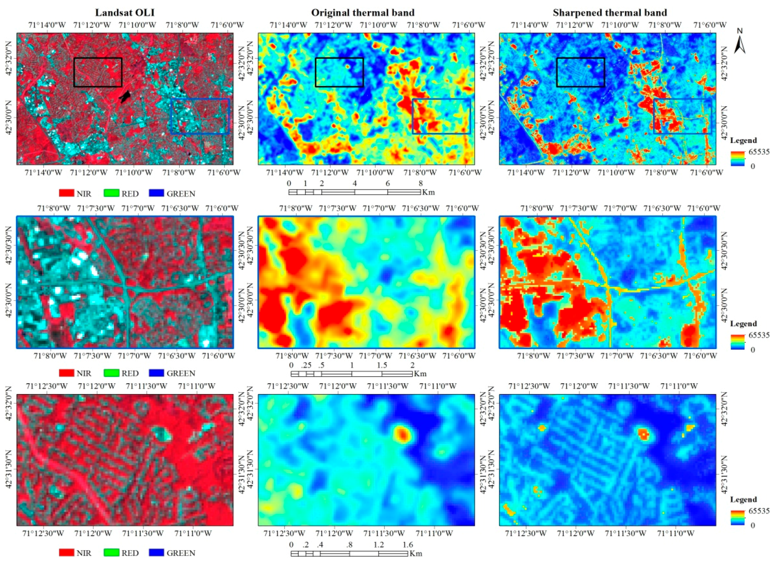
Figure 6.
The MNDISI histograms and the overall accuracy (OA) curves for summer images of: ETM+ (a,b); TM (c,d); and OLI (e,f). Their optimal thresholds are marked in each histogram, and the OA value using this threshold (red line) is positioned in the corresponding OA curve. The black line represents the threshold reaching the highest accuracy of ISA mapping.

Figure 7.
Comparison of seasonality between the MNDISI and NDISI using images from three sensors: (a) TM; (b) ETM+; and (c) OLI/TIRS.
Figure 7.
Comparison of seasonality between the MNDISI and NDISI using images from three sensors: (a) TM; (b) ETM+; and (c) OLI/TIRS.
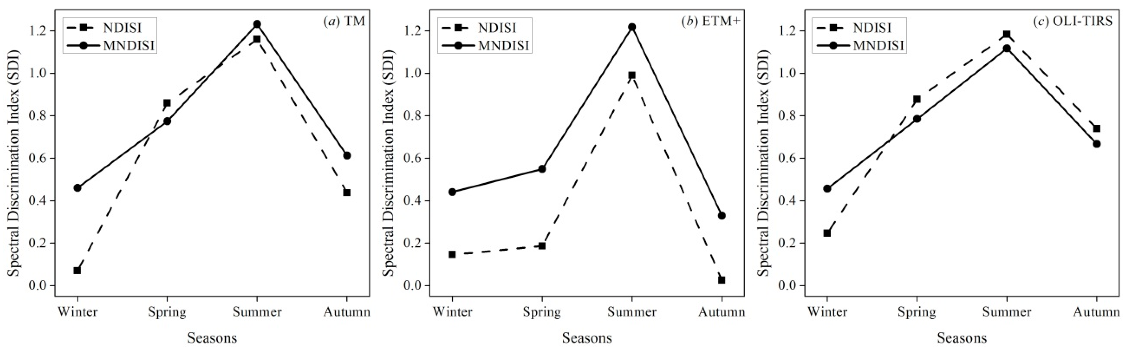
Figure 8.
The ISA distributions using: NDISI (a); and MNDISI (b), from the TM summer images.

Figure 9.
The ISA maps from the summer images in the four subsets of the study area: CBD (I); residential area (II); highway (III); and suburban–rural area (IV). The rows give: the standard false color image displays (a); the NLCD-extracted IS reference layers (b); the NDISI-extracted ISA maps (c); and the MNDISI-extracted maps (d).

Figure 10.
The IS and PS histograms and SDI values of the NDISI (left column) and MNDISI (right column) from summer images of: ETM+ acquired on 29 August 2001 (the first row); TM acquired on 30 August 2010 (the second row); and OLI/TIRS acquired on 13 July 2016 (the third row).
Figure 10.
The IS and PS histograms and SDI values of the NDISI (left column) and MNDISI (right column) from summer images of: ETM+ acquired on 29 August 2001 (the first row); TM acquired on 30 August 2010 (the second row); and OLI/TIRS acquired on 13 July 2016 (the third row).

Table 1.
Satellite images from the three Landsat sensors (TM, ETM+, OLI-TIRS) used in this study.
| Satellite | Sensor | Acquisition Date | Resolution (m) | Wavelength (μm) |
|---|---|---|---|---|
| Landsat-5 | TM | 24 April 2010 (spring) 30 August 2010 (summer) 5 November 2011 (autumn) 5 January 2011 (winter) | 30 | Band1 (Blue): 0.441–0.514 |
| Band2 (Green): 0.519–0.601 | ||||
| Band3 (Red): 0.631–0.692 | ||||
| Band4 (NIR): 0.772–0.898 | ||||
| Band5 (SWIR-1): 1.547–1.749 | ||||
| 120 | Band6 (TIR): 10.31–12.36 | |||
| 30 | Band7 (SWIR-2): 2.064–2.345 | |||
| Landsat-7 | ETM+ | 23 April 2001 (spring) 29 August 2001 (summer) 17 November 2001 (autumn) 1 January 2001 (winter) | 30 | Band1 (Blue): 0.441–0.514 |
| Band2 (Green): 0.519–0.601 | ||||
| Band3 (Red): 0.631–0.692 | ||||
| Band4 (NIR): 0.772–0.898 | ||||
| Band5 (SWIR-1): 1.547–1.749 | ||||
| 60 | Band6 (TIR): 10.31–12.36 | |||
| 30 | Band7 (SWIR-2): 2.064–2.345 | |||
| 15 | Band8 (Pan): 0.515–0.896 | |||
| Landsat-8 | OLI-TIRS | 24 April 2016 (spring) 13 July 2016 (summer) 30 October 2015 (autumn) 30 January 2016 (winter) | 30 | Band1 (Coastal/Aerosol): 0.435–0.451 |
| Band2 (Blue): 0.452–0.512 | ||||
| Band3 (Green): 0.533–0.590 | ||||
| Band4 (Red): 0.636–0.673 | ||||
| Band5 (NIR): 0.851–0.879 | ||||
| Band6 (SWIR-1): 1.566–1.651 | ||||
| Band7 (SWIR-2): 2.107–2.294 | ||||
| 15 | Band8 (Pan): 0.503–0.676 | |||
| 30 | Band9 (Cirrus): 1.363–1.384 | |||
| 100 | Band10 (TIR-1): 10.60–11.19 | |||
| Band11 (TIR-2): 11.50–12.51 |
Table 2.
Accuracy comparison between the NDISI and MNDISI classifications with the three summer images.
Table 2.
Accuracy comparison between the NDISI and MNDISI classifications with the three summer images.
| Built-up Indices | Accuracy Measures | TM | ETM+ | OLI-TIRS |
|---|---|---|---|---|
| NDISI | OA (%) | 84.64 | 85.77 | 84.19 |
| OK | 0.69 | 0.71 | 0.68 | |
| MNDISI | OA (%) | 89.35 | 87.19 | 87.52 |
| OK | 0.79 | 0.74 | 0.75 | |
| Improvement (MNDISI − NDISI) | OA (%) | 4.71 | 1.42 | 3.33 |
| OK | 0.10 | 0.03 | 0.07 |
© 2017 by the authors. Licensee MDPI, Basel, Switzerland. This article is an open access article distributed under the terms and conditions of the Creative Commons Attribution (CC BY) license (http://creativecommons.org/licenses/by/4.0/).
Share and Cite
MDPI and ACS Style
Sun, Z.; Wang, C.; Guo, H.; Shang, R. A Modified Normalized Difference Impervious Surface Index (MNDISI) for Automatic Urban Mapping from Landsat Imagery. Remote Sens. 2017, 9, 942. https://doi.org/10.3390/rs9090942
AMA Style
Sun Z, Wang C, Guo H, Shang R. A Modified Normalized Difference Impervious Surface Index (MNDISI) for Automatic Urban Mapping from Landsat Imagery. Remote Sensing. 2017; 9(9):942. https://doi.org/10.3390/rs9090942
Chicago/Turabian StyleSun, Zhongchang, Cuizhen Wang, Huadong Guo, and Ranran Shang. 2017. "A Modified Normalized Difference Impervious Surface Index (MNDISI) for Automatic Urban Mapping from Landsat Imagery" Remote Sensing 9, no. 9: 942. https://doi.org/10.3390/rs9090942
Note that from the first issue of 2016, this journal uses article numbers instead of page numbers. See further details here.