An Enhanced IT2FCM* Algorithm Integrating Spectral Indices and Spatial Information for Multi-Spectral Remote Sensing Image Clustering


1
School of Geographic and Environmental Sciences, Tianjin Key Laboratory of Water Resources and Environment, Tianjin Normal University, Tianjin 300387, China
2
Key Laboratory of Agricultural Remote Sensing, Ministry of Agriculture/Institute of Agricultural Resources and Regional Planning, Chinese Academy of Agricultural Sciences, Beijing 100081, China
*
Author to whom correspondence should be addressed.
Remote Sens. 2017, 9(9), 960; https://doi.org/10.3390/rs9090960
Submission received: 31 July 2017
/
Revised: 5 September 2017
/
Accepted: 13 September 2017
/
Published: 15 September 2017
(This article belongs to the Section Remote Sensing Image Processing)
Abstract
:Interval type-2 fuzzy c-means (IT2FCM) clustering methods for remote-sensing data classification are based on interval type-2 fuzzy sets and can effectively handle uncertainty of membership grade. However, most of these methods neglect the spatial information when they are used in image clustering. The spatial information and spectral indices are useful in remote-sensing data classification. Thus, determining how to integrate them into IT2FCM to improve the quality and accuracy of the classification is very important. This paper proposes an enhanced IT2FCM* (EnIT2FCM*) algorithm by combining spatial information and spectral indices for remote-sensing data classification. First, the new comprehensive spatial information is defined as the combination of the local spatial distance and attribute distance or membership-grade distance. Then, a novel distance metric is proposed by combining this new spatial information and the selected spectral indices; these selected spectral indices are treated as another dataset in this distance metric. To test the effectiveness of the EnIT2FCM* algorithm, four typical validity indices along with the confusion matrix and kappa coefficient are used. The experimental results show that the spatial information definition proposed here is effective, and some spectral indices and their combinations improve the performance of the EnIT2FCM*. Thus, the selection of suitable spectral indices is crucial, and the combination of soil adjusted vegetation index (SAVI) and the Automated Water Extraction Index (AWEIsh) is the best choice of spectral indices for this method.
1. Introduction
Land-use/land-cover (LULC) mapping using remote-sensing data is crucial. The main task of LULC mapping is to identify different land-use types by mapping multi-scale remote-sensing data. The fuzzy c-means (FCM) clustering [1] is a classical unsupervised soft clustering method and widely used in this domain because of its ability to handle fuzzy uncertainty. Classical FCM clustering methods are based on type-1 fuzzy set theory, which cannot address uncertainties associated with membership grade [2]. Some researchers adopt the interval type-2 fuzzy sets (IT2 FSs) to improve FCM clustering, and there are three strategies to avoid this problem: (1) The remote-sensing data expressed by real values are extended to interval numbers [3,4]. However, the widths of the intervals are difficult to determine because a single value must be related to an interval value, which can artificially increase the uncertainty in the data. (2) Hwang and Rhee [5] proposed the IT2FCM method using two fuzzifiers ( and ) and IT2 FS; this strategy is being extensively discussed. (3) The land-use types are classified by FCM with different fuzzifiers, and the results are integrated using IT2 FS [6]. Due to its ability to handle the uncertainty of membership values, the IT2FCM is widely used, and many derivative methods of IT2FCM have been developed, including the interval type-2 fuzzy possibilistic C-means (IFPCM) [7], interval-valued possibilistic fuzzy C-means (IPFCM) [8], general type-2 fuzzy C-means (GT2 FCM) [9], interval type-2 fuzzy C-means clustering with spatial information (IIT2-FCM) [10], and kernel interval-valued fuzzy C-Means (KIFCM) clustering algorithms [11]. As noted by Zarinbal et al. [12], in some of these methods, the type-2 fuzzy membership functions are defuzzified into type-1 fuzzy membership functions during each iteration, and the distances between a sample and cluster centers should be expressed as singleton values when used to calculate the lower and upper membership grades in a certain class; otherwise, in these cases, some information would be lost. However, beyond that, the spectrum of a geographic feature does not refer to a single spectral curve but rather to a connected set of possible spectral curves, namely, a spectral curve with a certain width [13]. To deal with the uncertainty in remote-sensing data, an interval type-2 fuzzy C-means clustering method based on the interval number distance (IND) and ranking, named the improved interval type-2 fuzzy c-means (IT2FCM*) clustering method, is proposed [14].
However, classical FCM clustering approaches suffer from a lack of spatial information at the pixel level. In other words, they rely on only the intensity distribution of the pixels and disregard their geometric information, which make them very sensitive to noise and other artifacts introduced during the imaging process [15]. To overcome this shortcoming, efforts have been made to integrate spatial information into FCM clustering, and the relevant methods can be grouped into three types: (1) those that integrate spatial information during each iteration, for example, the bias corrected FCM (BCFCM) [16] and Interval Type-2 Fuzzy C-Means clustering with spatial in- formation (IIT2-FCM) [10]; methods of this kind are of low efficiency; (2) those that integrate spatial information in the data processing step, such as the enhanced FCM (EnFCM) [17], the fast generalized FCM (FGFCM) [18] and the noise detecting FCM (NDFCM) [19], in which the spatial information is usually defined as the spatial similarity or gray similarity in a certain local window; with these methods, it is unnecessary to compute the neighbor information in each iteration; and (3) those that analyze the uncertainty in the FCM classification result and reclassify the pixels using a W × W window [20]. It is very difficult to strike a balance between the noise insensitivity and retention of image details or local contextual information [21], especially for remote-sensing images, because most pixels are made up of spectral features of different geographical objects in remote-sensing images; these are also called mixed pixels. Therefore, defining the spatial information is still a problem in remote-sensing classification.
Since the conceptual vegetation-impervious surface-soil triangle model proposed by Ridd [22] was first used in land-use/land-cover mapping with remote-sensing data, many spectral indices have been developed and widely used in applications, e.g., the normalized difference vegetation index (NDVI) [23], the soil adjusted vegetation index (SAVI) [24], the normalized difference water index (NDWI) [25], the normalized difference built-up index (NDBI) [26], the morphological building index (MBI), the morphological shadow index (MSI) [27], and the automated water extraction index (AWEI) [28]. Although these indices have proven effective in labeling special ground components [29,30,31], crucial problems can arise when they are applied to urban environments. The first problem is that most spectral indices are designed to highlight only a single land-cover type (e.g., vegetation or built-up area) and cannot differentiate among other land-cover types. The second problem of spectral indices is associated with their limited applicability in remote-sensing imagery at different spatial and spectral resolutions [32]. It is necessary to set threshold values for different spectral indices to segment different land-cover types in common methods [33,34,35]. However, it is difficult to find suitable threshold values. Thus, soft classification is another option, e.g., Yang et al. [36] discussed four combination scenarios of the modified FCM (MFCM) with water indices (WIs) and proposed a new surface water extraction method, the selected water index, which was treated as a special feature in MFCM.
The objective of the present study is to integrate the spatial information and spectral indices into the IT2FCM* method, and named as Enhanced IT2FCM* (EnIT2FCM*). The technical approach of this paper is shown in Figure 1. The Sentinel-2 dataset is used to test the EnIT2FCM* and ten bands of this dataset are selected; Section 4.1 will introduce this dataset in detail. The paper is organized as follows. In the next section, a brief introduction to spectral indices and spatial information used in FCMs is given and IT2FCM* is introduced. In Section 3, the main ideology for constructing the algorithm proposed in this paper is described. We construct a new spatial information description by membership degrees that is a combination of spatial similarity and membership value similarity. Then, the remotely sensed images are treated as one dataset source and the selected spectral indices as the other dataset source. A new distance is defined by these two datasets and spatial information. In Section 4, we further analyze this proposed method. As noted previously, spectral indices may be confused or in conflict with one another [32]; therefore, selecting suitable indices is critical. Thus, we compare different combinations of indices and then test the effectiveness of the new spatial information definition by comparing it with the existing definition. Validity indices for the EnIT2FCM* algorithm include PE-, PC-, XB- and FS-, and other indices such as the confusion matrix and kappa coefficients are also adopted to validate the classification results.
2. Preliminaries
Relevant preliminaries are presented in this section. In Section 2.1, some spatial information definitions are reviewed. In Section 2.2, the basic concept of IT2 FS is introduced. The IT2FCM* algorithm is introduced in Section 2.3.
2.1. Spatial Information in FCM
As noted in Section 1, spatial texture information is considered in FCMs, and many researchers have discussed this topic in the past two decades. We will review some typical spatial information definitions. In BCFCM [16], the objective function is defined as follows:
where C is the number of clusters, N is the number of pixels in dataset, are the centroids of all clusters, is the value of i-th pixel, represents the membership degree of j-th pixel to cluster i, Nj is the set of neighbors that exists in a window centered around j-th pixel and NR is the cardinality of Nj, is the value of r-th pixel in Nj and controls the effect of the spatial information. The neighbor information must be computed in each iteration, so its efficiency is low. Chen and Zhang [37] proposed FCMS1 and FCMS2 by replacing the spatial information with median-filtered and mean-filtered information respectively. In EnFCM, a linearly weighted sum image ξ is formed by the original image and its local neighbor average image in the data processing step:
where is the gray-level value of the i-th pixel of the image , Nj is the set of neighbors that exists in a window centered around j-th pixel and NR is the cardinality of Nj, the parameter α plays the same role as before. Because ξ is calculated during the data preprocessing, this algorithm runs faster than the algorithms that integrate spatial information during each iteration.
In FGFCM, a local similarity measure that combines both spatial and gray-level image information is defined as follows:
where the i-th pixel is the center of the local window and the j-th pixel represents the set of neighbors that fall within the local window around the i-th pixel, (pi, qi) is the coordinate of the i-th pixel, xi is its gray-level value, λs and λg are two scale parameters that play roles similar to that of parameter α in EnFCM, and σi is calculated as follows:
Then, a new image (linearly weighted sum image) ξ can be generated by the following:
where ξi be the gray-level value of the i-th pixel of the new image ξ. Then, the original image is replaced by ξ in this algorithm. Clearly, a pixel ξi in ξ no longer contains the intrinsic information xi because when I = j, Sij equals 0 in Equation (5). The algorithm proposed by Wang and Bu [38] has the same problem. It is common sense that spatial, textual and spectral information are the most important ones for human visual interpretation in remote-sensing image classification.
As some authors have noted, it is very difficult to strike a balance between noise insensitivity and image details. Previous works have proposed several methods to achieve this balance automatically; for example, Krinids and Chatzis proposed the fuzzy factor to express local spatial information in their fuzzy local information c-means (FLICM) algorithm [39]:
where the j-th pixel is the center of the local window, i is the reference cluster, the r-th pixel represents the set of neighbors that fall within the local window around the j-th pixel, djr is the spatial Euclidean distance between pixels r and j, is the membership degree of the r-th pixel to cluster i, vi is the center of cluster i, and m is the fuzzifier. Then, the objective function is expressed as follows:
Guo et al. [19] proposed the noise point probability for determining the balance parameters, which is expressed as follows:
where λα is a given parameter for controlling the scale and Ni and NR still represent the corresponding neighborhood window and the number of pixels in it, respectively. Then, the objective function is expressed as follows:
where ξi is the weighted mean computed according to (5) and is the mean of the corresponding neighborhood. Guo et al. claimed that the larger the difference between the central pixel and its surrounding pixels is, more likely it is that the pixel is a noise point [19].
Inspired by the method proposed by Cai et al. [18] and Krinids and Chatzis [39], Zhang et al. [21] proposed a novel algorithm based on the concept of pixel relevance. The pixel relevance between two pixels is measured by two image patches centered on them. Then, the fuzzy factor is inferred from the membership degree and remote-sensing dataset, and it is calculated during each iteration. However, this process neglects the spatial distance between the center pixel and its surrounding pixels, and it requires very high computational resources if the dataset has a large amount of attribute information, as is the case for hyperspectral images. Therefore, we propose a new spatial information definition in Section 3 to overcome these faults.
2.2. The Interval Type-2 Fuzzy Set
Fuzzy sets (i.e., type-1 fuzzy sets) have been applied to many domains because of their ability to model fuzziness [40]. However, fuzzy sets cannot manage the errors associated with the membership values of fuzzy objects. This flaw can be overcome by using type-2 fuzzy sets (T2 FS) and type-N fuzzy sets, which were introduced by Zadeh [41]. These shortcomings were recognized following the introduction and development of the type-1 fuzzy set theory, after which type-2 fuzzy set theory began to receive more attention. Some researchers provided a full comparison between type-1 and type-2 fuzzy sets and summarized the development and application of the latter [2,42].
A common type-2 fuzzy set features a non-interval secondary membership function, which makes computation extremely difficult. Additionally, the secondary membership value or function is difficult to handle. The interval type-2 fuzzy set (IT2 FS) is a special case of the T2 FS and many authors have referred to IT2 FS as T2 FS and added the qualifying term “generalized” only when discussing non-interval type-2 fuzzy sets [2]. The next portion of this section introduces concepts that are relevant to these interval type-2 fuzzy sets.
Definition 1 [43].
An interval type-2 fuzzy set X is a bivariate function on the Cartesian product, into [0,1], where is the universe for the primary variable x of . The point-valued representation of is
For the sake of convenience, the IT2 FS is represented as , and represents the membership value of the element x in .
2.3. IT2 FCM*
Two parameters that can be set by users are the number of classes C and the fuzzifier m [1] in the standard FCM method. The cluster centers are expressed by real-valued vectors, and the distances between a sample and the cluster centers are used to determine the membership grade of a sample belonging to a class. As noted above, classical FCM clustering methods cannot handle uncertainty of the membership degree. Hwang and Rhee proposed IT2FCM based on the IT2 FS to handle fuzziness uncertainty in fuzzy clustering [5]. The lower and upper membership functions are constructed using two fuzzifiers—m1 and m2, respectively—but IT2FCM and its extended algorithms, such as IIT2-FCM, still have some faults, which are discussed in Section 1. Thus, we proposed IT2FCM* based on the interval number distance and ranking [14].
There are multiple definitions of the distance between interval numbers. The Euclidean distance between interval numbers is commonly used, but its obvious fault is that this definition considers only endpoints of interval numbers [44]. We tested these distance definitions in IT2FCM* and proved that the definition proposed by Li et al. [45] is more effective than others. This definition is an extension of the definition proposed by Bertoluzza et al.
Let and be two interval numbers. Then, the interval distance between and is calculated as follows:
As in IT2FCM, the lower and upper membership functions are constructed using two fuzzifiers: and . Then, two objective functions can be established by Equations (12) and (13):
where is the distance metric between the sample and the cluster centroid , which is the interval vector distance based on Equation (11) and can be expressed as follows:
where is a sample; is an interval number vector; l = 1, 2, …, M; M is the number of features; C is the number of clusters; and N is the number of samples. These centroids are determined by the KM algorithm [46] during each iteration in IT2FCM*. Based on the IND methods and two different fuzziness parameters, i.e., and , the lower and upper membership grades of each sample can be expressed as follows:
The iteration can be stopped when is satisfied. Then, the lower and upper membership grades of each sample belonging to each class are determined, and they conform to an interval number vector . Then, the probability of any two intervals in the vector can be calculated as follows:
where and are the widths of the interval numbers and , respectively, for i, j = 1, 2, …, C and k = 1, 2, …, N.
We can then obtain a possibility matrix P = (pij, k). Moreover, the ranking vector can be calculated by , and the index of the maximum value in is the class index of the sample.
3. Methodology
As discussed above, the new spatial information and spectral indices are useful for remote-sensing data classification. In this section, we will incorporate these two types of dataset sources into the IT2FCM* and improve the IT2FCM* algorithm, which is called the EnIT2FCM* method here.
3.1. Spectral Indices
A spectral index is a ratio of two or more bands that have proven to be effective in LULC mapping. Unfortunately, some spectral indices have strong limitations on the data type or sensor type; for example, the worldview-2 sensor dataset has no SWIR band; thus, the AWEI indices cannot be used for it. We will review some commonly used indices in this section; a summary is provided in Table 1.
The MBI is selected in addition to the spectral indices in Table 1. These selected spectral indices can be classified into three types. NDVI, EVI and SAVI belong to vegetation indices (VIs); NDWI, MNDWI, AWEInsh and AWEIsh belong to the water indices (WIs); and NDBI, NDBaI, and MBI belong to the build indices (BIs). Yang et al. reported that the combinations of FCM with WIs can essentially be divided into four scenarios, and the scenario in which the WIs are regarded as newly generated bands achieves a balance between simplicity and effectiveness [36]. In this paper, we adopt this strategy to combine spectral indices. However, in addition to providing useful information, these spectral indices bring noise. For example, if we assume the threshold value is 0.05 for AWEIsh, a value greater than 0.05 will indicate a water body, which will enhance the classification, but a value less than 0.05 cannot indicate the correct land-cover type, resulting in noise. Although the most essential characteristic for discriminating a target object from its surrounding objects is the difference between their spectral curves, two problems are encountered. One is selecting which spectral indices or combinations to use in image clustering, and the other is setting the weights of these selected indices. This paper will propose a solution for these two problems in the EnIT2FCM* algorithm.
3.2. Spatial Information Measure
Usually, the spatial information in image classification mainly depends on both the local geometric relationship and the attributive relationship. The local geometric relationship is measured by the spatial Euclidean distances between the central pixel and its surrounding pixels in a local window; the closer the distance, the higher the similarity. The local attributive relationship is measured by the distances between the attributes of the central pixel and its surround pixels. Let the size of the local window be . Then, we can define a comprehensive distance by combining the local spatial distance and attribute distance based on Equation (4):
where is the spatial distance between central pixel k and surrounding pixel h in its neighbor window and is the distance based on the attribute or membership degree; the Euclidean distance is adopted in this paper. Our experiment shows that the attribute of a pixel or membership degree of a pixel belonging to a certain class can be used to measure the local attributive relationship, and a similar result can be produced.
Then, the spatial information measure can be defined as follows:
where are the lower and upper membership grades, respectively, of a pixel belonging to class i.
3.3. The enhanced IT2FCM*
When taking spectral indices and spatial information into account, the dataset X of images is constructed with the original dataset Y and the selected spectral indices Z. Then, the corresponding class centers can be expressed as and . A new distance between pixel k and centroid i is proposed, which combines spectral information, the spectral indices of itself and the spatial information from surrounding pixels. This new distance can be expressed as follows:
where is the interval distance defined by Equation (4); more specifically, is the spectral attribute distance of a pixel k to the spectral attribute center of class i, and is the spectral index distance of a pixel k to a spectral index center of class i. is the spatial information and is calculated by Equation (19), is the parameter that controls the relative impact of the spatial information in the local window; if , the spatial information is not taken into account. The parameter controls the effect of selected spectral indices. Theoretically, the selected spectral indices could be used for classification directly; thus, is not limited to values less than 1. If and at the same time, then the algorithm reduces to the IT2FCM* algorithm.
4. Experimental Results and Discussion
In this section, we will use the Sentinel-2 dataset to test the EnIT2FCM* algorithm. The study area is classified into five types: building, bare land, grass, wood and water body. Here, the fuzzifiers and are set to 2.1 and 5, respectively. The effects of spatial information and spectral indices are discussed in the following, and their combined effect is also described.
4.1. Data Set and Study Area
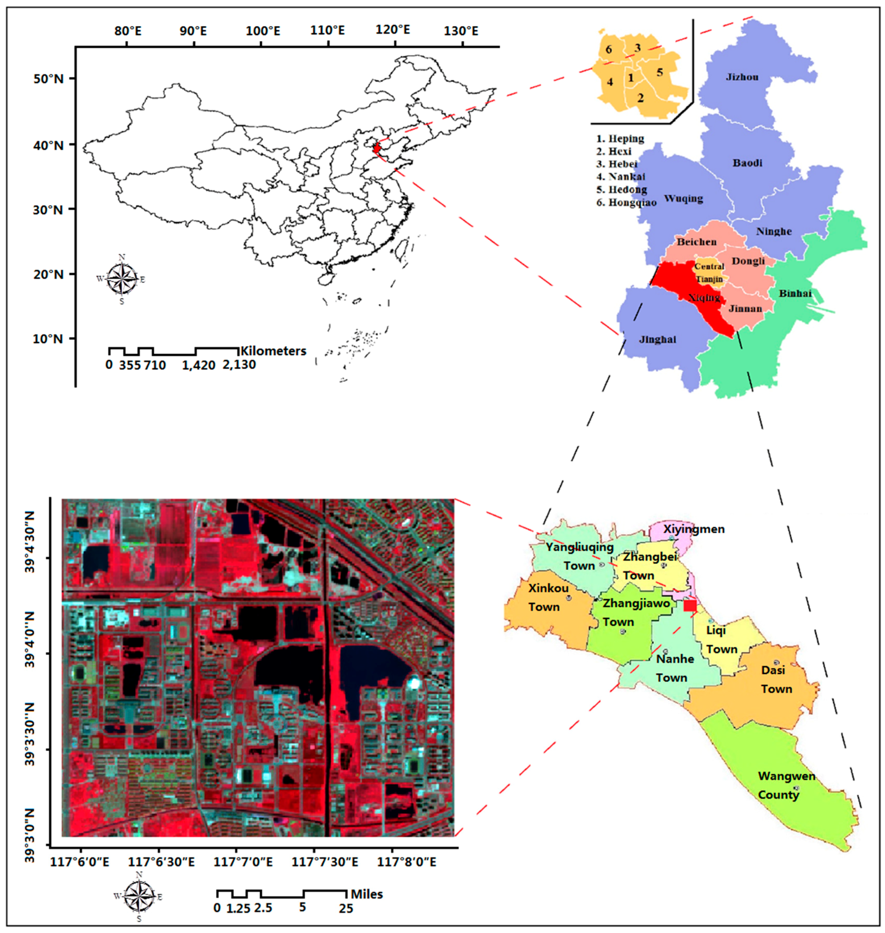
The study area is located in southwestern Tianjin City, a metropolis in northern coastal Mainland China and one of the five national central cities of the country, with a latitude ranging from 38°34′ to 40°15′ N and a longitude ranging from 116°43′ to 118°04′ E (see Figure 3). Three universities are included within the study area: Tianjin Normal University, Tianjin Poly Technique University, and the Tianjin University of Technology. The reason for choosing this region as the study area for this research is mainly the convenience for validation. The land cover of this study area is mainly composed of buildings, ponds, trees, grassland, trails, and concrete roads.
In this paper, a cloud-free multispectral high-resolution image from the Sentinel-2 satellite, which was acquired on 28 August 2016, is used for classification to test the classification ability of the improved EnIT2FCM* algorithm presented in this paper. Sentinel-2A was launched on 23 June 2015. It is a polar-orbiting, multispectral high-resolution imaging mission for land monitoring to provide, for example, imagery of vegetation, soil and water cover, inland waterways and coastal areas. The spectral region ranges from 0.44 to 2.2 µm, with 13 spectral channels in the visible, near-infrared, and short-wave-infrared parts of the spectrum. Among these 13 bands, there are 3 channels, which are designed for detecting coastal aerosol (0.443 µm), water vapor (0.945 µm), and cirrus (1.375 µm), with a spatial resolution of 60 m. The spatial resolution of visible bands 2 to 4 (spectral region ranging from 0.490 to 0.665 µm) and NIR band 8 (0.842 µm) is 10 m, and the spatial resolution of bands 5 to 7 (ranging from 0.705 to 0.783 µm), band 8 (0.865 µm) and bands 11 and 12 (with wavelengths of 1.610 µm and 2.190 µm, respectively) is 20 m. The acquired dataset is a Level-1C product, which is the top-of-atmosphere (TOA) radiance data. This product is currently processed using a processor running on European Space Agency’s (ESA’s) Sentinel-2 Toolbox. Before the classification, the necessary preprocessing was carried out for the multispectral images to convert the Level-1C product into a Level-2A product, which is the bottom-of-atmosphere (BOA) reflectance data, for further classification. This step is mainly performed by the SNAP software and its plug-in component CEN2COR, which are provided on the official website of the ESA.
4.2. The Effect of Spatial Information
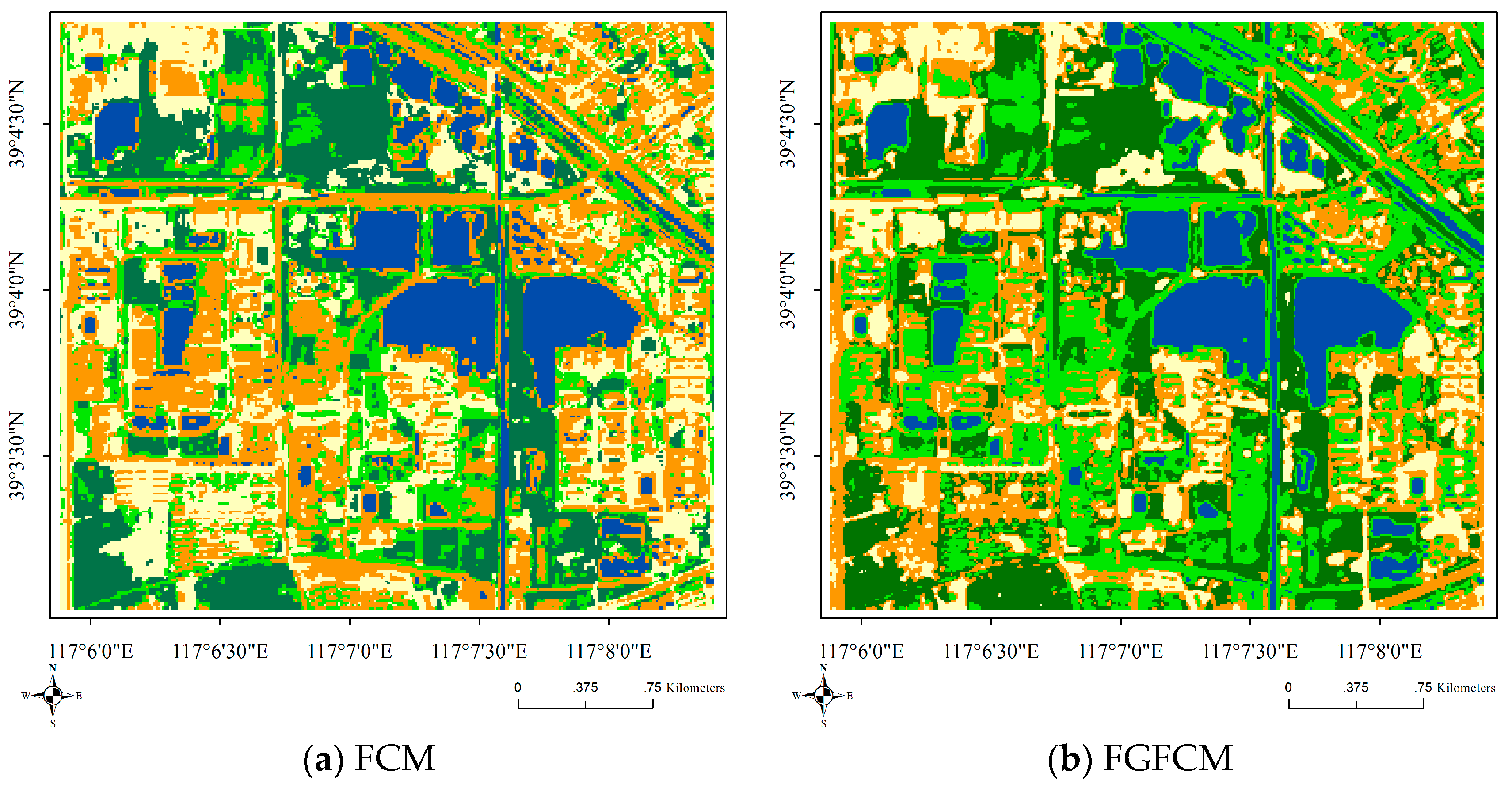
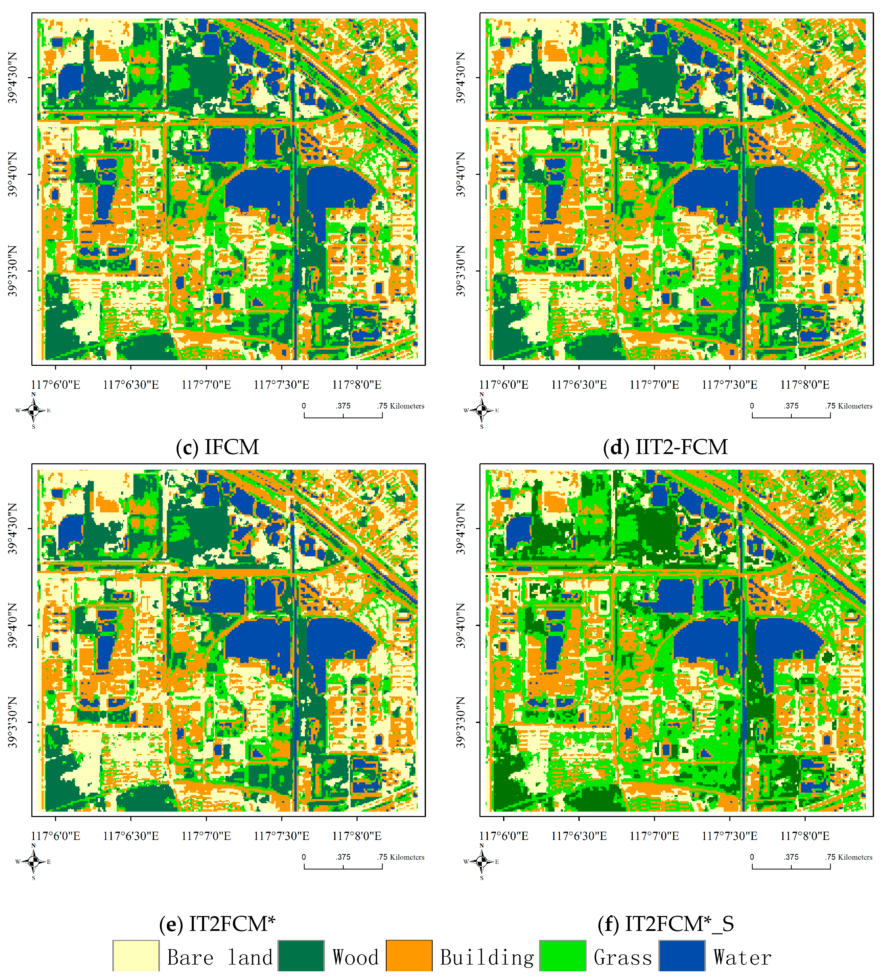
The main work of this subsection is to perform a comparative analysis between the spatial information definition (FGFCM) of Cai et al. [18], the definition (IIT2-FCM) of Ngo et al., [10] and the definition (IT2FCM*_S) proposed in the present paper. The size of the local window is . Four typical validity indices for type-1 fuzzy clustering are selected in this research: the partition coefficient (PC-), the partition entropy (PE-), the Fukuyama and Sugeno index (FS-), and the Xie and Beni index (XB-) [51]. During the process, the parameter is set to 1 and the corresponding error coefficient is set to 0.001. We know that the value of PC- indicates the average relative amount of membership sharing between pairs of fuzzy subsets. The higher the PC- value is, the better the corresponding classification results will be. PE- is a scalar measure of the amount of fuzziness in a set of results, and FS- is designed to measure the discrepancy between fuzzy compactness and fuzzy separation. XB- is used to measure the average within-cluster fuzzy compactness against the minimum between-cluster separation. The values of these three indices are smaller, indicating better clustering performance of these clustering methods.
In Table 3, comparing the indices of FCM, IFCM, IT2FCM*, FGFCM, IIT2-FCM and IT2FCM*_S, all of these spatial information definitions improvthe corresponding results. IT2FCM* with spatial information yields the maximum value of PC- and the minimum values of PE- and FS-. Although the XB- value of IT2FCM*_S is not the smallest, it still indicates that spatial information improves the performance of EnIT2FCM*. Figure 4 shows the classification results of these methods; the pictures also illustrate this conclusion.
4.3. The Effect of Spectral Indices
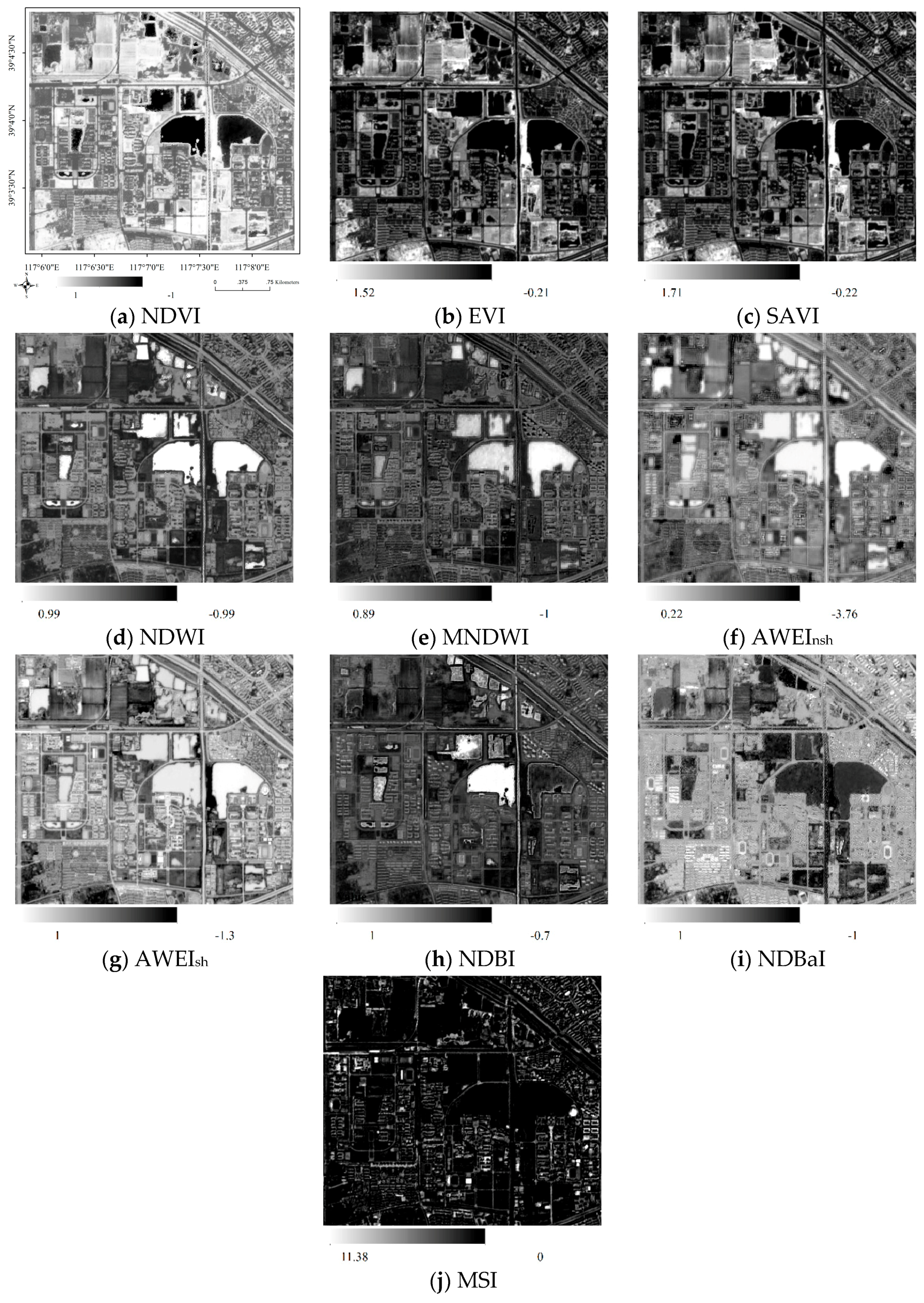
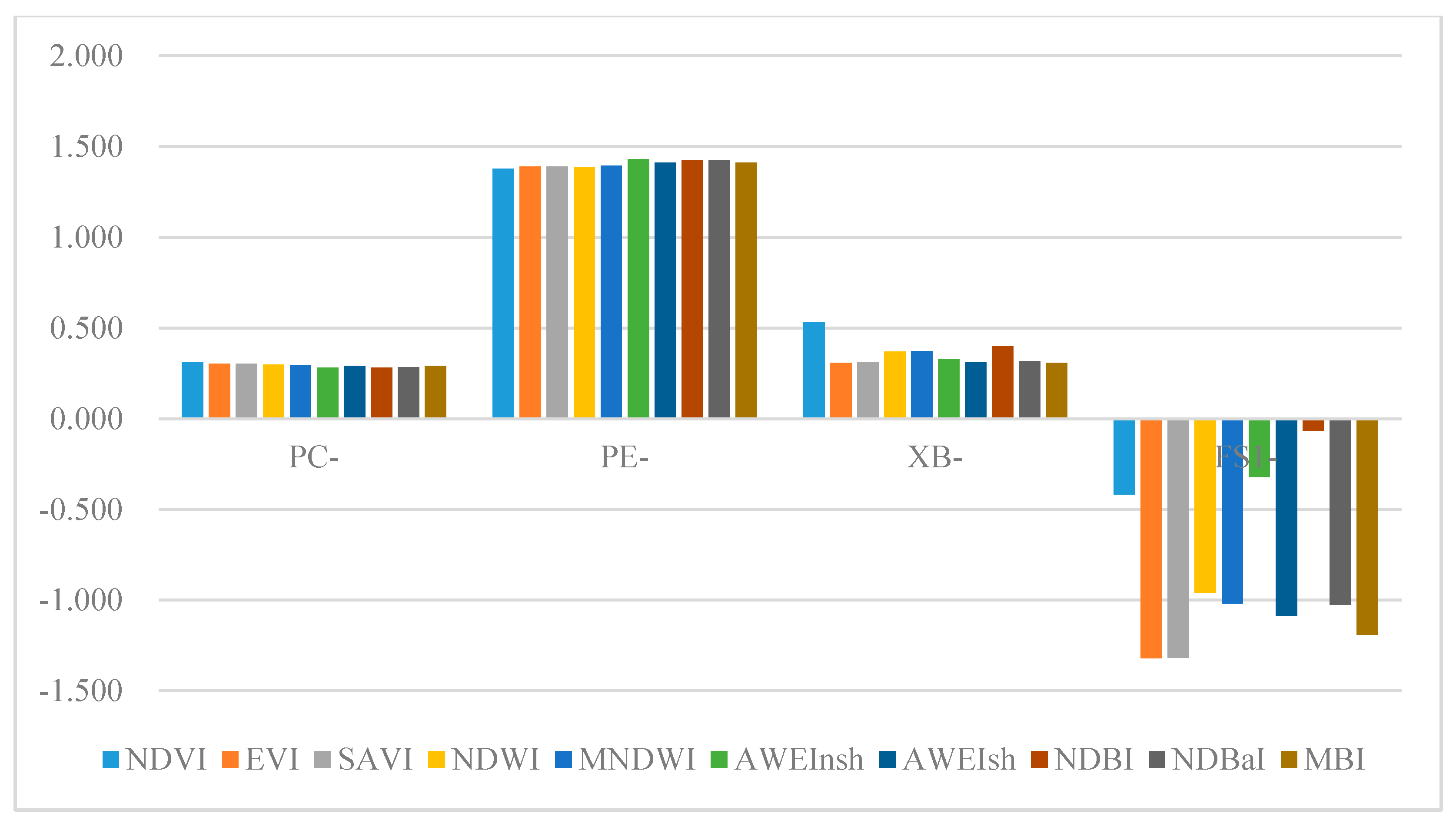
In this section, we will test the performance of spectral indices in EnIT2FCM*. As noted above, spectral indices may provide useful information as well as noise. Selection of suitable spectral indices is crucial. The strategy adopted in this paper includes three steps. The first step is to calculate the spectral indices listed in Table 1; the results are shown in Figure 5. The second step is to integrate these indices into Equation (20) one by one and test the validity indices PC-, PE-, XB- and FS-; the results are shown in Figure 6.
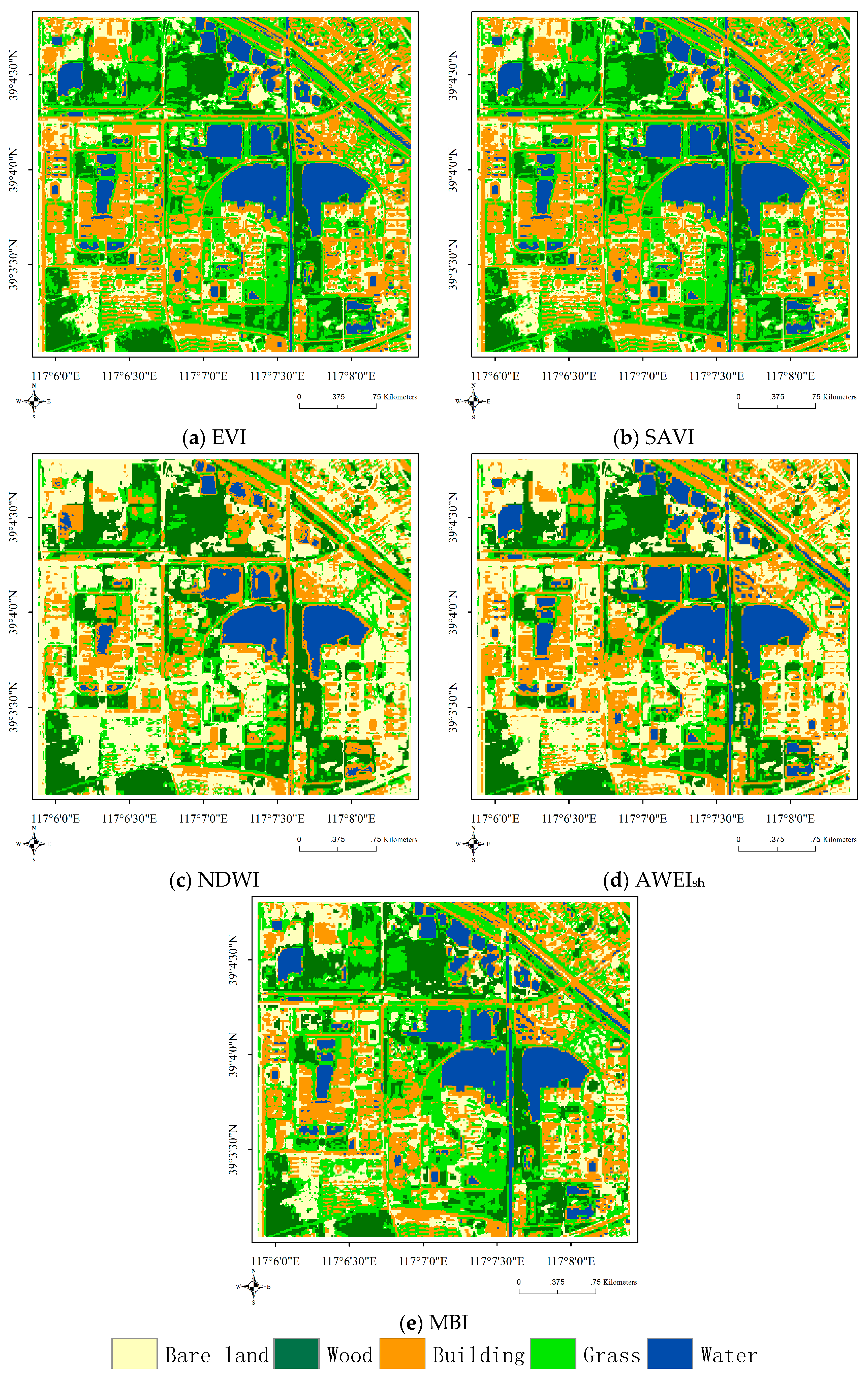
For these validity indices, when NDVI is used, the maximum value of PC- can be achieved; when the AWEInsh is used, the minimum value of PC- can be achieved; the maximum and minimum values of PE- can be achieved when AWEInsh is used; and the minimum value of PE- can be achieved when NDVI is used. The maximum and minimum values of XB- can be achieved using NDVI and EVI, respectively. The maximum and minimum values of FS- can be achieved using NDBI and EVI, respectively. Regarding the VIs, the results of EVI and SAVI are similar, while NDVI achieves perfect values of PC- and PE- but poor values of XB- and FS-. Regarding the WIs, AWEIsh is superior to the others overall. Regarding the BIs, MBI is better than NDBI and NDBaI, and NDBI has the worst performance of all of these spectral indices. The classification results of EnIT2FCM* combined with a single spectral index are shown in Figure 7. In Figure 7, we can see that two vegetation indices (EVI and SAVI) improve the classification very well, as shown in Figure 7a,b. However, NDWI performs poorly (Figure 7c); we can see that the river is classified as bare land, and some buildings are also classified as bare land. AWEIsh and MBI can improve classification but still have some problems; for example, some buildings are classified as bare land by AWEIsh, and bare land is wrongly classified as wooded areas, as shown in Figure 7d,e, respectively.
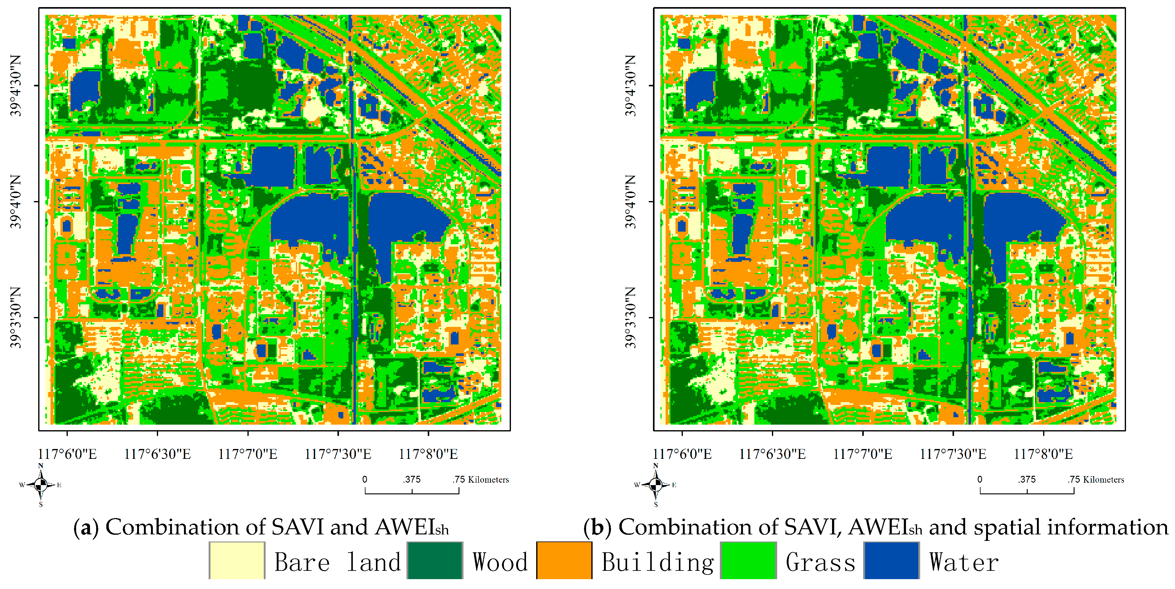
Next, a variety of combinations of different indices are built and integrated into Equation (20) one by one to test the PC- and PE-. It should be noted that some validity indices, such as FS- and XB-, cannot be used because their dimensions are not equal; therefore, the confusion matrix and kappa coefficient are adopted here. We tested more than 30 representative combinations among them according to the analysis of Step 1, and then eight combinations are selected for discussion here. We can see that Combination 6 (see column ID in Table 4) has the best validity effect because it has the greatest PC- value and minimum PE- value; however, the overall accuracy and kappa coefficient values are poor. Combination 1 has the optimal user accuracy and kappa coefficient value, but its PC- and PE- values are not very good. Combination 7 has the worst performance among these indices, which indicates that the excessive combination of spectral indices does not improve the classification accuracy. To some extent, it may degrade the classification accuracy. Combination 1 has the best performance overall in terms of accuracy and kappa coefficient and relatively better performance in terms of PC- and PE-; thus, in this step, the combination of SAVI and AWEIsh is regarded as the best combination, as shown in Figure 8a. The difference between Combinations 1 and 4 is that Combination 4 has one more spectral index, MBI, than Combination 1. However, the performance of these indices is not as good as that of combination 1, and the same situation occurs with Combination 5. Thus, we conclude that combining suitable spectral indices in IT2FCM* will improve the classification performance.
4.4. Combination Effect of Spatial Information and Spectral Indices
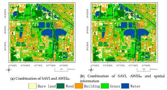
In Section 4.2, we tested the effects of spatial information on four validity indices and showed that the spatial information measure proposed in this paper achieves good performance. In Section 4.3, we found that EnIT2FCM* with the combination of SAVI and AWEIsh has the best performance. In this subsection, we will test the combination effect of spatial information and spectral indices SAVI and AWEIsh; the results are shown in Figure 8b. Four validity indices, namely, PC-, PE-, XB- and FS-, along with the accuracy and kappa coefficient are adopted here. We set and , and other parameters are set to the same values as before. PC-, PE-, XB- and FS- are equal to 0.301, 1.39, 0.308 and −1.16 × 10⁷, respectively, when considering the effect of these two indices. When the spatial information and these two spectral indices are used in the EnIT2FCM* algorithm at the same time, values of the validity indices improve: 0.313, 1.37, 0.278 and −1.58 × 10⁷, respectively. The overall accuracy and kappa coefficient are also improved, from 87.92% and 0.843 to 88.02% and 0.844, respectively.
4.5. Discussion
In this section, an experiment is implemented to test the EnIT2FCM*. The spatial information definition proposed in this paper combines spatial distance and attribute distance, and it has been shown to have very good performance, so it is more comprehensive than the method proposed by Ngo et al. [10]. Although some other definitions consider the spatial information and attribution information, and the attribute information is based on pixel value, e.g., EnFCM [17], FGFCM [18], and NDFCM [19]. When these methods are used for multispectral or hyperspectral remote sensing classification, the number of bands is relatively large, then the amount of calculation may be relatively large. Thus, the definition proposed in this paper provides another choice in these situations. In other words, we can use the membership value to calculate the attribute distance if the number of classification is smaller than the number of bands.
As mentioned before, few works consider spectral indices in FCMs for remote sensing classification and Yang et al. [36] has made a good start, but this work only considered the water indices. This paper makes a full investigation about common vegetation indices, water indices and build indices, the experiment shows that EVI, SAVI and AWEIsh have better performance in these indices, and then the combination of SAVI and AWEIsh has been discovered that it has the best performance than single spectral index or other combinations in this experiment.
When taking the combination of spatial information and spectral indices into account, this combination still improves the classification accuracy, although the magnitude of the improvement is not particularly obvious. However, overall, the combination effect of spatial information and suitable spectral indices with the modified IT2FCM* improves the classification accuracy significantly.
5. Conclusions
Classification of remote-sensing data is crucial in remote-sensing domain, especially in the era of big data. Spectral attributes, spectral indices and spatial information are important for classification. Usually, spectral attributes and spectral indices can be used to classify or segment a remote-sensing image individually, and the spatial information of an image is usually used to improve the performance. This paper attempts to incorporate these factors into the classification algorithm. First, a new distance metric is defined for this target, after which the EnIT2FCM* is proposed, which is a type of unsupervised classification method and an extension of IT2FCM*. Experimental results showed that the spatial information definition proposed here is effective and improves the classification performance. Some spectral indices and their combinations improve the performance of this enhanced IT2FCM*. The combination of SAVI and AWEIsh is the best choice of spectral indices in this method. However, an improper spectral index will degrade the classification accuracy; therefore, the selection of suitable spectral indices is crucial in this method. The combination effect of spatial information and suitable spectral indices with the EnIT2FCM* improves the classification accuracy significantly.
The distance metric has a crucial impact on the FCM. As mentioned in Section 1, the spectral characteristic curves of nearly all geographical features should be bands with certain ranges, and the centers of each class are defined as interval vectors in the IT2FCM* and enhanced IT2FCM*; therefore, the measurement of the distances from a pixel to these interval vectors is still a problem. Thus, in future research, we will investigate different distance metrics for these algorithms. In addition, the optimal spectral index may be different for different remote-sensing data. Existing spectral indices are generally induced from Landsat datasets; whether these spectral indices can be applied to other remote-sensing data, such as WorldView-3, needs to be studied in depth, and this problem is still crucial for the EnIT2FCM*. Therefore, determining the validity of spectral indices for different types of remote-sensing data and possibly defining new spectral indices for different types of remote-sensing data are among our future research priorities.
Acknowledgments
The work in this paper was supported by grants from the Chinese National Nature Science Foundation (No. 41101352), the Key Project of Tianjin Natural Science Foundation of China (17JCZDJC39700) and the China Postdoctoral Science Foundation (2016 M601181).
Author Contributions
Jifa Guo conceived and designed the research, implemented the EnIT2FCM* algorithm in Java and wrote the manuscript. Hongyuan Huo analyzed all test results and revised the manuscript.
Conflicts of Interest
The authors declare no conflicts of interest.
References
- Bezdek, J.C.; Ehrlich, R.; Full, W. FCM: The fuzzy c-means clustering algorithm. Comput. Geosci. 1984, 10, 191–203. [Google Scholar] [CrossRef]
- John, R.; Coupland, S. Type-2 fuzzy logic: A historical view. IEEE Comput. Intell. Mag. 2007, 2, 57–62. [Google Scholar] [CrossRef]
- De Carvalho, F.D.A.T.; Tenório, C.P. Fuzzy K-means clustering algorithms for interval-valued data based on adaptive quadratic distances. Fuzzy Sets Syst. 2010, 161, 2978–2999. [Google Scholar] [CrossRef]
- Yu, X.; He, H.; Hu, D.; Zhou, W. Land cover classification of remote sensing imagery based on interval-valued data fuzzy c-means algorithm. Sci. China Earth Sci. 2014, 57, 1306–1313. [Google Scholar] [CrossRef]
- Hwang, C.; Rhee, F.C.H. Uncertain fuzzy clustering: Interval type-2 fuzzy approach to C-means. IEEE Trans. Fuzzy Syst. 2007, 15, 107–120. [Google Scholar] [CrossRef]
- Fisher, P.F. Remote sensing of land cover classes as type 2 fuzzy sets. Remote Sens. Environ. 2010, 114, 309–321. [Google Scholar] [CrossRef]
- Min, J.; Shim, E.A.; Rhee, F.C.H. An interval type-2 fuzzy PCM algorithm for pattern recognition. In Proceedings of the 18th International Conference on Fuzzy Systems, Jeju Island, Korea, 20–24 August 2009; pp. 480–483. [Google Scholar]
- Ji, Z.; Xia, Y.; Sun, Q.; Cao, G. Interval-valued possibilistic fuzzy C-means clustering algorithm. Fuzzy Sets Syst. 2014, 253, 138–156. [Google Scholar] [CrossRef]
- Ondrej, L.; Milos, M. General Type-2 fuzzy C-Means algorithm for uncertain fuzzy clustering. IEEE Trans. Fuzzy Syst. 2012, 20, 883–897. [Google Scholar]
- Ngo, L.T.; Mai, D.S.; Pedrycz, W. Semi-supervising Interval Type-2 Fuzzy C-Means clustering with spatial information for multi-spectral satellite image classification and change detection. Comput. Geosci. 2015, 83, 1–16. [Google Scholar] [CrossRef]
- Nguyen, D.D.; Ngo, L.T.; Pham, L.T.; Pedrycz, W. Towards hybrid clustering approach to data classification: Multiple kernels based interval-valued Fuzzy C-Means algorithms. Fuzzy Sets Syst. 2015, 279, 17–39. [Google Scholar] [CrossRef]
- Zarinbal, M.; Fazel Zarandi, M.H.; Turksen, I.B. Interval type-2 relative entropy fuzzy C-means clustering. Inf. Sci. 2014, 272, 49–72. [Google Scholar] [CrossRef]
- Swain, P.H.; Davis, S.M. Remote Sensing: The Quantitative Approach; McGraw-Hill: New York, NY, USA, 1978. [Google Scholar]
- Guo, J.; Huo, H.; Xiong, G. Interval Type-2 Fuzzy C-Means Clustering based on Interval Number Distance and Ranking. Fuzzy Sets Syst. 2017, in press. [Google Scholar]
- Wang, Z.; Song, Q.; Soh, Y.; Sim, K. An adaptive spatial information-theoretic fuzzy clustering algorithm for image segmentation. Comput. Vis. Image Underst. 2013, 117, 1412–1420. [Google Scholar] [CrossRef]
- Ahmed, M.N.; Yamany, S.M.; Mohamed, N.; Farag, A.A.; Moriarty, T. A modified fuzzy C-mean algorithm for bias field estimation and segmentation of MRI data. IEEE Trans. Med. Imaging 2002, 21, 193–199. [Google Scholar] [CrossRef] [PubMed]
- Szilágyi, L.; Benýo, Z.; Szilágyii, S.M.; Adam, H.S. MR Brain image segmentation using an enhanced fuzzy C-means algorithm. In Proceedings of the IEEE 25th Annual International Conference of the Engineering in Medicine and Biology Society, Cancun, Mexico, 17–21 September 2003. [Google Scholar]
- Cai, W.; Chen, S.; Zhang, D. Fast and robust fuzzy C-means clustering algorithms incorporating local information for image segmentation. Pattern Recogn. 2007, 40, 825–838. [Google Scholar] [CrossRef]
- Guo, F.; Wang, X.; Shen, J. Adaptive fuzzy c-means algorithm based on local noise detecting for image segmentation. IET Image Process. 2016, 10, 272–279. [Google Scholar] [CrossRef]
- Wang, Q.; Shi, W. Unsupervised classification based on fuzzy c-means with uncertainty analysis. Remote Sens. Lett. 2013, 4, 1087–1096. [Google Scholar] [CrossRef]
- Zhang, X.; Sun, Y.; Wang, G.; Guo, Q.; Zhang, C.; Chen, B. Improved fuzzy clustering algorithm with non-local information for image segmentation. Multimedia Tools Appl. 2017, 76, 7869–7895. [Google Scholar] [CrossRef]
- Ridd, M. Exploring a V-I-S (vegetation-impervious-surface-soil) model for urban ecosystem analysis through remote sensing: Comparative anatomy for cities. Int. J. Remote Sens. 1995, 16, 2165–2185. [Google Scholar] [CrossRef]
- Rouse, J.W.; Haas, R.; Schell, J. Monitoring the Vernal Advancement and Retrogradation (Green Wave Effect) of Natural Vegetation; Texas A&M University: College Station, TX, USA, 1974. [Google Scholar]
- Huete, A.R. A soil-adjusted vegetation index (SAVI). Remote Sens. Environ. 1988, 25, 295–309. [Google Scholar] [CrossRef]
- McFeeters, S.K. The use of Normalized Difference Water Index (NDWI) in the delineation of open water features. Int. J. Remote Sens. 1996, 17, 1425–1432. [Google Scholar] [CrossRef]
- Zha, Y.; Gao, Y.; Ni, S. Use of normalized difference built-up index in automatically mapping urban areas from TM imagery. Int. J. Remote Sens. 2003, 24, 583–594. [Google Scholar] [CrossRef]
- Huang, X.; Zhang, L. Morphological Building/Shadow Index for Building Extraction from High-Resolution Imagery over Urban Areas. IEEE J. Sel. Top. Appl. Earth Obs. Remote Sens. 2012, 5, 161–172. [Google Scholar] [CrossRef]
- Feyisa, G.; Meilby, L.H.; Fensholt, R.; Proud, S.R. Automated Water Extraction Index: A new technique for surface water mapping using Landsat imagery. Remote Sens. Environ. 2014, 140, 23–35. [Google Scholar] [CrossRef]
- Du, Y.; Zhang, Y.; Ling, F.; Wang, Q.; Li, W.; Li, X. Water Bodies’ Mapping from Sentinel-2 Imagery with Modified Normalized Difference Water Index at 10-m Spatial Resolution Produced by Sharpening the SWIR Band. Remote Sens. 2016, 8, 354. [Google Scholar] [CrossRef] [Green Version]
- Li, Y.; Gong, X.; Guo, Z.; Xu, K.; Hu, D.; Zhou, H. An index and approach for water extraction using Landsat–OLI data. Int. J. Remote Sens. 2016, 37, 3611–3635. [Google Scholar] [CrossRef]
- Wen, D.; Huang, X.; Liu, H.; Liao, W.; Zhang, L. Semantic Classification of Urban Trees Using Very High Resolution Satellite Imagery. IEEE J. Sel. Top. Appl. Earth Obs. Remote Sens. 2107, 10, 1413–1424. [Google Scholar] [CrossRef]
- Deng, C.; Wu, C. BCI: A biophysical composition index for remote sensing of urban environments. Remote Sens. Environ. 2012, 127, 247–259. [Google Scholar] [CrossRef]
- Drăguţ, L.; Csillik, O.; Eisank, C.; Tiede, D. Automated parameterisation for multi-scale image segmentation on multiple layers. ISPRS J. Photogramm. Remote Sens. 2014, 88, 119–127. [Google Scholar] [CrossRef] [PubMed]
- Xie, H.; Luo, X.; Xu, X.; Pan, H.; Tong, X. Evaluation of Landsat 8 OLI imagery for unsupervised inland water extraction. Int. J. Remote Sens. 2016, 37, 1826–1844. [Google Scholar] [CrossRef]
- Zhou, Y.; Dong, J.; Xiao, X.; Xiao, T.; Yang, Z.; Zhao, G.; Zou, Z.; Qin, Y. Open Surface Water Mapping Algorithms: A Comparison of Water-Related Spectral Indices and Sensors. Water 2017, 9, 256. [Google Scholar] [CrossRef]
- Yang, Y.; Liu, Y.; Zhou, M.; Zhang, W.; Sun, C.; Duan, Y. Landsat 8 OLI image based terrestrial water extraction from heterogeneous backgrounds using a reflectance homogenization approach. Remote Sens. Environ. 2015, 171, 14–32. [Google Scholar] [CrossRef]
- Chen, S.; Zhang, D. Robust image segmentation using fcm with spatial constraints based on new kernel-induced distance measure. IEEE Trans. Syst. Man Cybern. Part B Cybern. 2004, 34, 1907–1916. [Google Scholar] [CrossRef]
- Wang, X.; Bu, J. A fast and robust image segmentation using FCM with spatial information. Digit. Signal Process. 2010, 20, 1173–1182. [Google Scholar] [CrossRef]
- Krinidis, S.; Chatzis, V. A Robust Fuzzy Local Information C-means Clustering Algorithm. IEEE Trans. Image Process. 2010, 19, 1328–1337. [Google Scholar] [CrossRef] [PubMed]
- Zadeh, L.A. Fuzzy Sets. Inf. Control 1965, 8, 338–353. [Google Scholar] [CrossRef]
- Zadeh, L.A. The concept of a linguistic variable and its application to approximate reasoning—I. Inf. Sci. 1975, 8, 199–249. [Google Scholar] [CrossRef]
- Oscar, C.; Patricia, M. Type-2 Fuzzy Logic: Theory and Applications; Springer: Berlin/Heidelberg, Germany, 2008. [Google Scholar]
- Mendel, J.M.; John, R.I.B. Type-2 fuzzy sets made simple. IEEE Trans. Fuzzy Syst. 2002, 10, 117–127. [Google Scholar] [CrossRef]
- Bertoluzza, C.; Corral, N.; Salas, A. On a new class of distances between fuzzy numbers. Mathw. Soft Comput. 1995, 2, 71–84. [Google Scholar]
- Li, X.; Zhang, S. Rank of interval numbers based on a new distance measure. J. Xihua Univ. (Nat. Sci.) 2008, 27, 87–90. [Google Scholar]
- Karnik, N.N.; Mendel, J.M. Applications of type-2 fuzzy logic systems to forecasting of time-series. Inf. Sci. 1999, 120, 89–111. [Google Scholar] [CrossRef]
- Jiang, Z.; Huetea, A.R.; Didan, K.; Miura, T. Development of a two-band enhanced vegetation index without a blue band. Remote Sens. Environ. 2008, 112, 3833–3845. [Google Scholar] [CrossRef]
- Xu, H. Modification of normalised difference water index (NDWI) to enhance open water features in remotely sensed imagery. Int. J. Remote Sens. 2006, 27, 3025–3033. [Google Scholar] [CrossRef]
- Zha, Y.; Ni, S.; Yang, S. An effective approach to automatically extract urban land-use from TM Imagery. J. Remote Sens. 2003, 7, 37–40. [Google Scholar]
- Zhao, H.M.; Chen, X.L. Use of normalized difference bareness index in quickly mapping bare areas from TM/TM+ imagery. In Proceedings of the Geoscience and Remote Sensing Symposium, Seoul, Korea, 29 July 2005. [Google Scholar]
- Wang, W.; Zhang, Y. On fuzzy cluster validity indices. Fuzzy Sets Syst. 2007, 158, 2095–2117. [Google Scholar] [CrossRef]
Figure 1.
Diagram of the technical approach of this paper.

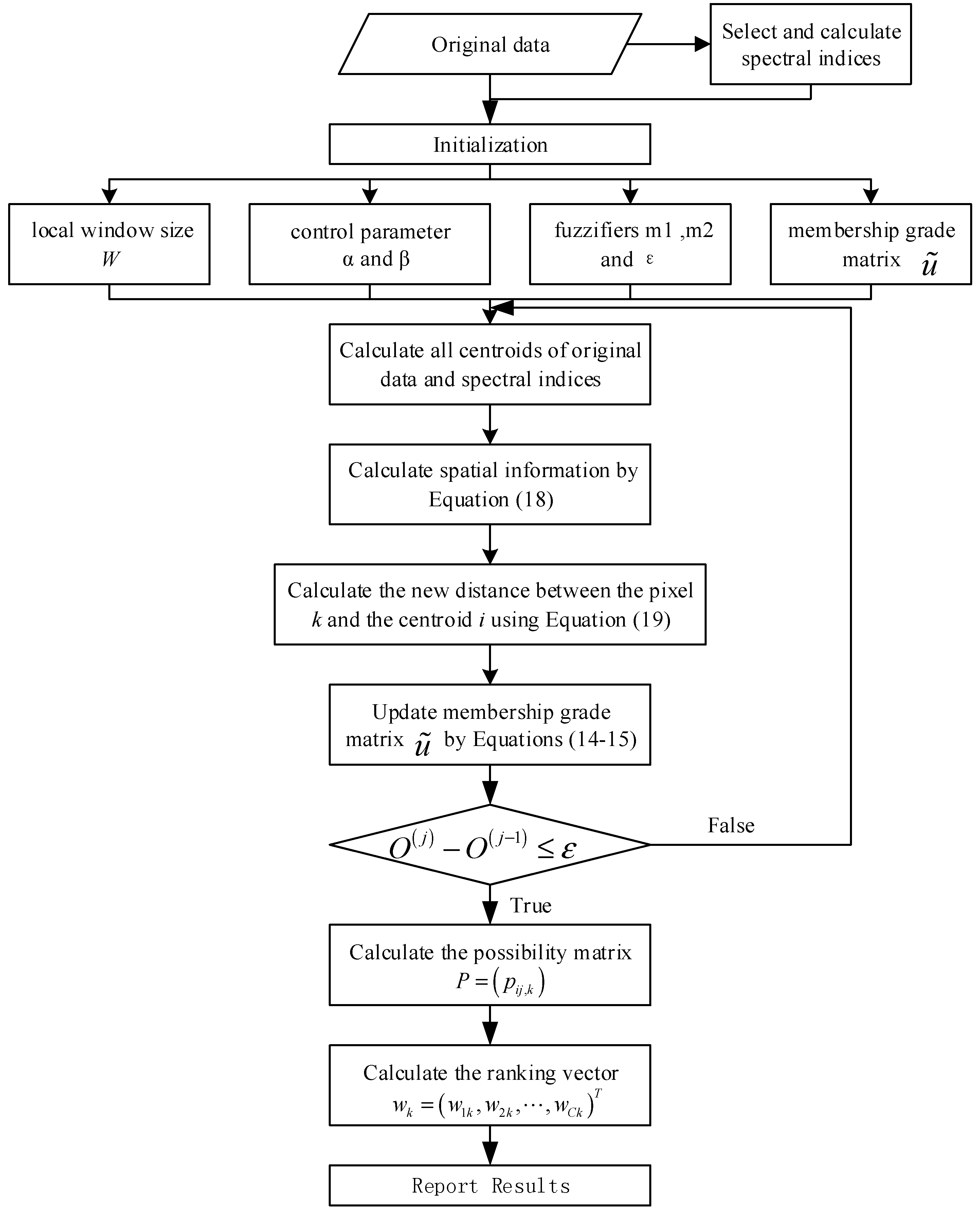
Figure 2.
Diagram of the EnIT2FCM* algorithm.

Figure 3.
The study area.

Figure 4.
Classification results of IT2FCM* and IT2FCM*_S.


Figure 5.
Spectral indices of the research area.

Figure 6.
Validity indices of EnIT2FCM* integrating different single spectral indices.

Figure 7.
Classification results of EnIT2FCM* by combining single spectral indices.

Figure 8.
Classification results of EnIT2FCM* by combining with SAVI and AWEIsh.


Table 1.
Some commonly used spectral indices.
| Index | Equation | Remarks |
|---|---|---|
| NDVI [23] | ||
| EVI [47] | ||
| SAVI [24] | L = 0.5 | |
| NDWI [25] | ||
| MNDWI [48] | ||
| AWEInsh [28] | ||
| AWEIsh [28] | ||
| NDBI [49] | ||
| NDBaI [50] | Thermal Infrared |
In Table 1, BLU, GREEN, RED, NIR, SWIR1, SWIR2 and TIR are the reflectance values of blue, green red, nir, swir1, swir2 and thermal infrared band, respectively.
Table 2.
The process of the EnIT2FCM*.
| Main Steps | Detail Steps |
|---|---|
| Step 1. Initialization | 1.1 Select suitable spectral indices according to the sensor type, research area, and major surface types, and then calculate these indices by suitable bands. |
| 1.2 Select the local window size W, usually , and then set values of control parameters and . | |
| 1.3 Select the parameters and () and the termination criterion value ε. | |
| 1.4 Initialize the lower and upper membership grade matrix using a random method. | |
| Step 2. Compute all centroids of the original data and selected spectral indices and then calculate the spatial information and update the membership grade matrix. | 2.1 Calculate all centroids of the original data = 1, 2, …, C and spectral indices and determine their lower and upper bands and , respectively, via the KM algorithm. |
| 2.2 Calculate the comprehensive distance using Equation (18) and spatial information using Equation (19). | |
| 2.3 Calculate the new distance between the pixel k and the centroid i using Equation (20). | |
| 2.4 Update the lower and upper membership grade matrix using Equations (15) and (16). | |
| 2.5 Calculate the objective function via Equation (3). If , go to step 3; otherwise, go to step 2. | |
| Step 3. Classify each sample using the interval number ranking method. | 3.1 Calculate the possibility matrix using Equation (16) and then obtain the ranking vector. |
| 3.2 Assign a sample to a cluster. | |
| 3.3 Report the clustering results. |
Table 3.
Typical validity indices for FCM, IFCM, IT2FCM*, FGFCM, IIT2-FCM and IT2FCM*_S.
| Index | FCM | IT2FCM | IT2FCM* | FGFCM | IIT2-FCM | IT2FCM*_S |
|---|---|---|---|---|---|---|
| PC- | 0.258 | 0.261 | 0.295 | 0.274 | 0.267 | 0.308 |
| PE- | 1.478 | 1.415 | 1.405 | 1.446 | 1.395 | 1.380 |
| XB- | 0.633 | 0.280 | 0.305 | 0.599 | 0.257 | 0.282 |
| FS- | −6.212 × 10⁶ | −8.433 × 10⁶ | −1.279 × 10⁷ | −6.990 × 10⁷ | −1.173 × 10⁷ | −1.707 × 10⁷ |
Table 4.
Results of PC-, PE- and accuracy of enhanced IT2FCM* combining different spectral indices.
| ID | Spectral Indices | PC- | PE- | Overall Accuracy | Kappa Coefficient |
|---|---|---|---|---|---|
| 1 | SAVI, AWEIsh | 0.301 | 1.393 | 87.92% | 0.843 |
| 2 | EVI, AWEIsh | 0.314 | 1.369 | 78.06% | 0.698 |
| 3 | EVI, SAWEIsh, MBI | 0.304 | 1.393 | 77.13% | 0.700 |
| 4 | SAVI, AWEIsh, MBI | 0.299 | 1.398 | 87.65% | 0.839 |
| 5 | SAVI, AWEIsh, NDBaI | 0.293 | 1.409 | 86.49% | 0.825 |
| 6 | NDVI, SAVI, NDWI | 0.320 | 1.355 | 73.22% | 0.653 |
| 7 | EVI, SAVI, NDWI, MBI, AWEInsh, AWEIsh, NDBaI | 0.288 | 1.419 | 74.25% | 0.666 |
| 8 | NDVI, NDWI, NDBaI | 0.310 | 1.373 | 68.65% | 0.591 |
© 2017 by the authors. Licensee MDPI, Basel, Switzerland. This article is an open access article distributed under the terms and conditions of the Creative Commons Attribution (CC BY) license (http://creativecommons.org/licenses/by/4.0/).
Share and Cite
MDPI and ACS Style
Guo, J.; Huo, H. An Enhanced IT2FCM* Algorithm Integrating Spectral Indices and Spatial Information for Multi-Spectral Remote Sensing Image Clustering. Remote Sens. 2017, 9, 960. https://doi.org/10.3390/rs9090960
AMA Style
Guo J, Huo H. An Enhanced IT2FCM* Algorithm Integrating Spectral Indices and Spatial Information for Multi-Spectral Remote Sensing Image Clustering. Remote Sensing. 2017; 9(9):960. https://doi.org/10.3390/rs9090960
Chicago/Turabian StyleGuo, Jifa, and Hongyuan Huo. 2017. "An Enhanced IT2FCM* Algorithm Integrating Spectral Indices and Spatial Information for Multi-Spectral Remote Sensing Image Clustering" Remote Sensing 9, no. 9: 960. https://doi.org/10.3390/rs9090960
Note that from the first issue of 2016, this journal uses article numbers instead of page numbers. See further details here.