Temporal Interpolation of Satellite-Derived Leaf Area Index Time Series by Introducing Spatial-Temporal Constraints for Heterogeneous Grasslands


1
School of Information Engineering, China University of Geosciences, Beijing 100083, China
2
School of Geographical Sciences, Northeast Normal University, Changchun 130024, China
*
Author to whom correspondence should be addressed.
Remote Sens. 2017, 9(9), 968; https://doi.org/10.3390/rs9090968
Submission received: 2 August 2017
/
Revised: 16 September 2017
/
Accepted: 18 September 2017
/
Published: 19 September 2017
(This article belongs to the Special Issue Land Surface Phenology )
Abstract
:Continuous satellite-derived leaf area index (LAI) time series are critical for modeling land surface process. In this study, we present an interpolation algorithm to predict the missing data in LAI time series for ecosystems with high within-ecosystem heterogeneity, particularly heterogeneous grasslands. The algorithm is based on spatial-temporal constraints, i.e., the missing data in the LAI time series of a pixel are predicted by the phenological links with other pixels. To address the uncertainties in the construction and selection of reference curves in a heterogeneous landscape, the algorithm constructs a reference dataset for each missing data in the LAI time series from all pixels showing very strong linear phenological links with the target pixel within a region. We also use an iterative process to update the available spatial-temporal constraints. We tested the algorithm with an eight-day composite Moderate Resolution Imaging Spectroradiometer (MODIS) LAI product in the Songnen grasslands, Northeast China in 2010 and 2011. The validation dataset was generated based on high quality time series by artificially adding data gaps. The algorithm achieved high overall interpolation accuracies with high coefficient of determination R2 (>0.9) and low root mean square error (RMSE) (<0.2) in both dry (2010) and wet (2011) years. The algorithm showed advantages in predicting missing data for different seasons and proportions of missing data versus the algorithm that uses regional average LAI curve as a reference. These results suggest that the proposed algorithm could more effectively characterize spatial-temporal constraint information in heterogeneous grasslands for temporal interpolation.
1. Introduction
As a key biophysical variable that controls terrestrial ecosystem processes (e.g., exchange of energy, water, and carbon), leaf area index (LAI) time series are critical for ecosystem and climate modeling [1,2,3]. Global high temporal resolution (four or eight days) LAI products are being produced with the Terra and Aqua MODIS observations. Although the released LAI products are multiday composited to minimize the effects of abiotic factors, there are still low quality data mainly due to persistent cloud, high aerosol, and snow cover during the composite period, as well as the limitations of the LAI retrieval method [4]. These low quality data in the LAI time series masks the real canopy dynamics and hinders its continuous monitoring, for example in the monitoring of phenological events [5,6].
A number of satellite-derived time series reconstruction methods have been developed, for instance, the Savitzky–Golay filter [7], the Fourier analysis [8,9,10,11], the wavelet transform [12,13,14], and function fitting [15,16]. These algorithms have shown their efficiencies for smoothing time series in diverse ecosystems [17,18,19,20,21,22]. However, they may not perform well for time series with less high-quality observations. The abilities of these algorithms for reconstructing time series are limited by insufficient temporal information.
Filling gaps in the time series of a pixel by using spatial and temporal constraints around the pixel (ecosystem-dependent interpolation, EDI) is an alternative strategy [23,24,25,26,27,28]. The basic assumption behind the EDI method is that in a region with limited surface variation, pixels belonging to the same ecosystem generally show strong phenological links because of the similar climate and soil conditions, and the missing data in the time series of a pixel can be filled based on the links with other pixels [23]. To some degree, the EDI method could overcome the lack of temporal information in a gap by introducing spatial information. The key issue of the EDI method is to construct and select appropriate reference time series. In [23], multiscale (from 0.5° × 0.5° to 10° × 10°) average surface albedo time series for an ecosystem were generated as candidates. The selection of reference time series depends on its match degree with the target pixel. While in [25] the best successfully fitted LAI curve with asymmetric Gaussian function within a window was selected as reference time series. The window can vary from about 10 km × 10 km to 1° × 1°. If successfully fitted LAI curve was not found, then the MODIS tile level average LAI time series for the same ecosystem was used. It is reasonable for homogeneous ecosystems to select only one reference curve from other pixels or regional average curve in [23,25]. However, these algorithms are likely to show limitation in ecosystems with high within-ecosystem heterogeneity. For example, degraded grasslands may exhibit significantly diverse phenological behaviors due to different community compositions even within a small region with similar climate conditions. Hence, the regional average curve or a curve from surrounding pixel may not strongly correlate to the seasonal curve of the target pixel. In this case, the strategy to select reference curve in [23,25] will bring in uncertainties in predicting missing data. Vegetation continuous field has been used to reduce the influence of within-ecosystem heterogeneity in [24]. However, the addressed heterogeneity in [24] is mainly caused by mixed pixel (vegetation and bare soil). The strategy is not suitable for pixel-level heterogeneity because the vegetation continuous field cannot characterize the heterogeneity caused by vegetation communities (e.g., degraded grasslands at different succession stages). On the other hand, it can be argued that a reference time series from function fitting may not be appropriate for middle-high latitude or alpine grasslands. First, growing season is generally short in these ecosystems. Second, vegetation growth in grasslands generally does not show an ideal S-shape due to its sensitivity to environmental factors, especially drought. Although more complex functions have been employed to consider stress conditions [29,30], the limited number of high-quality observations from multiday composite product in an annual time series may not support a statistically reliable fitting to the improved logistic functions or the asymmetric Gaussian function [31]. If neither the fitted nor the average time series is used, there may not exist a complete LAI time series that can be selected as reference for a pixel because each LAI time series may have missing data. This requires a more flexible strategy to predict the missing data.
In this study, we improved the EDI method proposed by Moody et al. [23] to address the uncertainties in interpolating missing data in satellite-derived LAI time series for heterogeneous landscape, particularly heterogeneous grasslands. We refer to the algorithm as the Enhanced Ecosystem-Dependent Interpolation (EEDI). The EEDI algorithm constructs a reference time series set for each missing data in the time series of a pixel from pixels showing very strong phenological links with the target pixel within a region. An iterative process is adopted to update the spatial-temporal reference information. Performance of the EEDI algorithm was compared with the EDI algorithm that directly uses a regional average LAI curve as reference [23].
2. Materials and Methods
2.1. Test Area
The algorithm was tested with grasslands in the Songnen plain, Northeast China. Due to the human activities, climate, geology, and terrain conditions, these mid-latitude semi-arid grasslands are salinized and alkalized at various degrees [32,33,34]. As a result, the Songnen grasslands are at different succession stages with diverse community compositions and, hence, show a typically heterogeneous landscape. We selected a 100 km × 100 km window in the Songnen plain as the test area (Figure 1a). Grasslands were extracted from the MODIS Collection 5 Land Cover-type product with the International Geosphere Biosphere Programme (IGBP) classification scheme. There are about 15,000 grasslands pixels in the test area. The distribution of the growing season’s mean LAI in 2011 displays the heterogeneity of the grasslands in the test area (Figure 1b).
2.2. MODIS LAI Product
For this analysis we selected the MODIS Collection 6 combined Terra and Aqua LAI product (MCD15A2H) because it is considered to have the highest quality among the MODIS LAI products [4]. The MCD15A2H product uses both Terra and Aqua reflectance observations as inputs to estimate daily LAI at 500 m spatial resolution, and an eight-day composite is performed to reduce the noise from abiotic factors [4]. To evaluate the performance of our algorithm for years under different meteorological conditions, we selected the LAI data in 2010 and 2011. Annual precipitations in the test area between these two years are significantly different (about 320 mm and 450 mm in 2010 and 2011, respectively). For each year, data only from late April (day of year 113) to mid-October (day of year 289) were analyzed because during other period vegetation is under dormancy and snow cover often exists in the area. Consequently, there are 23 available images per year.
2.3. Algorithm Development
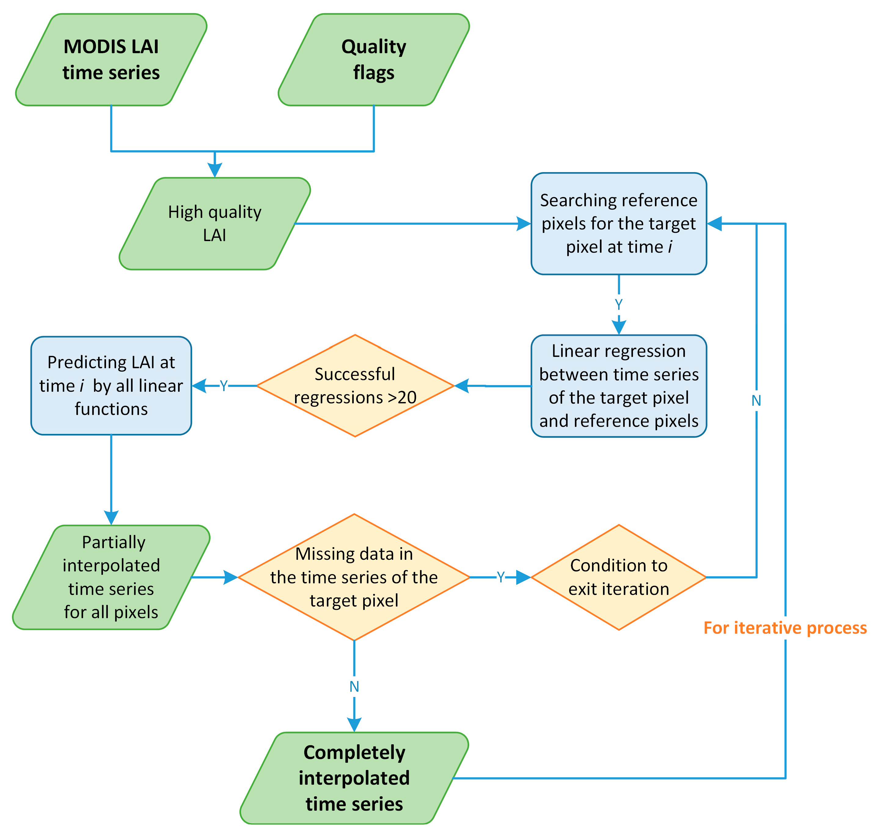
An overview of the algorithm is provided in Figure 2. In general, the algorithm includes two major steps: (1) preprocessing of raw LAI time series with the aid of quality flags, and (2) filling gaps using the phenological links between the LAI time series of the target pixel and the reference pixels.
2.3.1. Extracting High Quality LAI Data
The MODIS MCD15A2H product includes two data quality control layers (a general layer and a detailed layer) that provide valuable information to extract high quality observations from the original LAI time series. A summary of the selected items from the quality layers for determining high quality data are given in Table 1. Observations in LAI time series flagged as cloud, cloud shadow, cirrus, and snow are first removed. The five-level confidence score provided by the general layer evaluates the reliability of LAI value in terms of the used LAI retrieval method. In this study, only LAI estimated from the main method, i.e., the Look-Up Table (LUT) method [35], is identified as high quality. Since the input reflectance data (MOD09GA and MCD09GA) of the MCD15A2H LAI product are atmospherically corrected, effects of low and average aerosol on LAI estimation are considered to be negligible. The effect of high aerosol should be taken into account because it may not be completely removed in the atmospheric correction process. Unfortunately, flags of average and high aerosol are provided together in the detailed quality layer. We, therefore, developed an alternative strategy to determine if an observation in LAI time series is contaminated by high aerosol. As high aerosol generally results in an abnormally low NDVI value, an observation contaminated by high aerosol will, therefore, show a drop in an LAI time series. Hence, if an observation is at a trough in an LAI time series and is flagged as average or high aerosol, it is considered to be affected by high aerosol. Furthermore, if several neighboring observations have the same LAI value during the growing season (LAI > 0.3), only the first one is identified as high quality because change in grasslands is generally rapid. An observation with extremely high LAI value, i.e.,, here μ is the mean and σ is the standard deviation of an LAI time series, is considered as noise. Such abnormal high value may be caused by sensor disturbances [17]. All data identified as low quality are removed, and will be predicted with the reserved high quality data. In addition, time series with too few high quality observations (less than 30%, eight points in this study) are discarded.
2.3.2. Temporal Interpolation of LAI Time Series with Phenological Links
The following steps are developed to predict the missing data in the LAI time series of a pixel (,), where is time, is the LAI value, i = 1, 2, …, n. n is 23 in this study.
Step 1: For a missing at , the algorithm searches pixels that have high quality LAI at within a given search radius around the target pixel. In heterogeneous landscape, searching all available pixels within a region is a solution to increase the chance of finding pixels that have strong phenological links with the target pixel. The search radius in this study is 25 km. This search range is close to a typical climate modeling grid of 0.05°. We refer to the LAI time series of the searched pixels in this step as candidate time series for the target pixel.
Step 2: Linear regression is performed between the target pixel’s time series and each candidate time series with all of the matching high quality data pairs throughout a time window. The generated linear functions are used to quantify the phenological links between the target pixel and the candidate pixels. A small time window can capture local variations but may not provide sufficient points to support reliable and stable regression. Since the growing season is short in our test area, the time window in this study covers the whole growing season, i.e., from to . In addition, regression will not be performed under two conditions: First, the number of the high quality data pairs is less than 30% (eight points). This is to avoid generating a regression function with low statistical power, although it may show high coefficient of determination. Second, the difference between and the nearest point to in the high quality data pairs is greater than 16 days. The criterion is formulated to ensure that the local variations in LAI near are considered in the regression.
Step 3: A regression function with the coefficient of determination R2 > 0.95 is considered as successful regression. A successful regression means the candidate time series show strong phenological links with the target pixel’s time series, and the candidate time series are selected as one of the reference time series. To reduce uncertainties in estimating , the following calculations are only performed if there are more than 20 successful regressions. For each successful regression, the algorithm predicts an LAI value by Equation (1):
where and are the slope and intercept of the regression function, respectively. is the LAI value at of the reference time series, and is a predicted LAI value at . The final LAI value at is averaged from the predicted LAI values with all successful regression functions.
Step 4: A new LAI dataset that has less missing data can be generated after performing the above three steps for all pixels in the region. The new dataset is then examined to determine whether there are remaining missing data. If missing data are found for a pixel, steps 1–3 are re-executed for this pixel. This iterative process is important in our algorithm to update the available spatial-temporal constraint information for a pixel. The iterative process is terminated until it reaches a given condition, such as an iteration times or no missing data is found. To avoid significant error accumulation, the initial iteration times in this study is two. If there are more than 10% incomplete time series within the region after the two iterations, another iteration with relaxed criteria is then performed. In this iteration, the required number of successful regression is pulled down to ten. After the iterative process has been terminated, the remaining incomplete time series with more than 15 points are interpolated by the cubic spline interpolation. The other incomplete time series are not further processed.
2.4. Algorithm Validation and Comparison
We adopt the strategy that uses high quality time series to generate validation dataset by artificially creating data gaps [19,20,28]. This is a widely used strategy to quantify the performance of time series reconstruction algorithms. We first randomly selected about 50% high-quality time series (more than 80% (18) high quality observations) in the test area as validation time series. We then randomly removed 1–14 high quality observations from each validation time series to create validation dataset with different proportions of missing data. We made sure the selected LAI time series after this process still contain more than eight high quality observations. These removed observations were used as validation data and their LAI values will be predicted by our algorithm. Interpolation accuracies were evaluated by directly comparing the predicted LAI with the original LAI for different proportions of missing data (PMD) and seasons of missing data (SMD) for each year. Four indicators were used: the R2, root mean square error (RMSE), slope, and intercept of the linear regression between the predicted LAI and the validation data. The R2 and RMSE are the major evaluation indicators.
We compared the EEDI algorithm with the EDI algorithm that uses multiscale regional average time series as candidate reference time series [23]. The radiuses of the EDI algorithm are 15 km and 25 km in this study. To reduce uncertainties in calculating the regional average time series, the LAI value of each point in the regional average time series must be averaged from more than 50 pixels. The regional average time series may also have missing data. If so, cubic spline interpolation is used to generate a complete reference time series, which is mandatory in the EDI algorithm. For the two regional average time series, the one shows a stronger phenological link (linear regression with higher R2) with the time series of the target pixel is selected as reference time series. The missing data were then predicted with the corresponding linear regression function.
3. Results
3.1. Determination of Iteration Times
Most of the pixels’ LAI time series have 12–16 high quality observations (PMD 30–50%) after removing the low quality data in both dry and wet years (Figure 3). In 2011, about 79% and 93% pixel’s time series were completely filled (23 points) after the first and second iterations, respectively. Iterative process was therefore terminated after the two iterations for data in 2011. In 2010, the proportions were about 60% and 75%, respectively. The last iteration with the relaxed criteria only produced another 6% complete time series in 2010. The results suggest that three iterations for this region is appropriate. The incomplete time series after three iterations are more likely to belong to a unique ecosystem, have suffered disturbance, or be contaminated by noise. Therefore, they did not exhibit strong phenological links with other time series within the region.
3.2. Effects of PMD on Interpolation
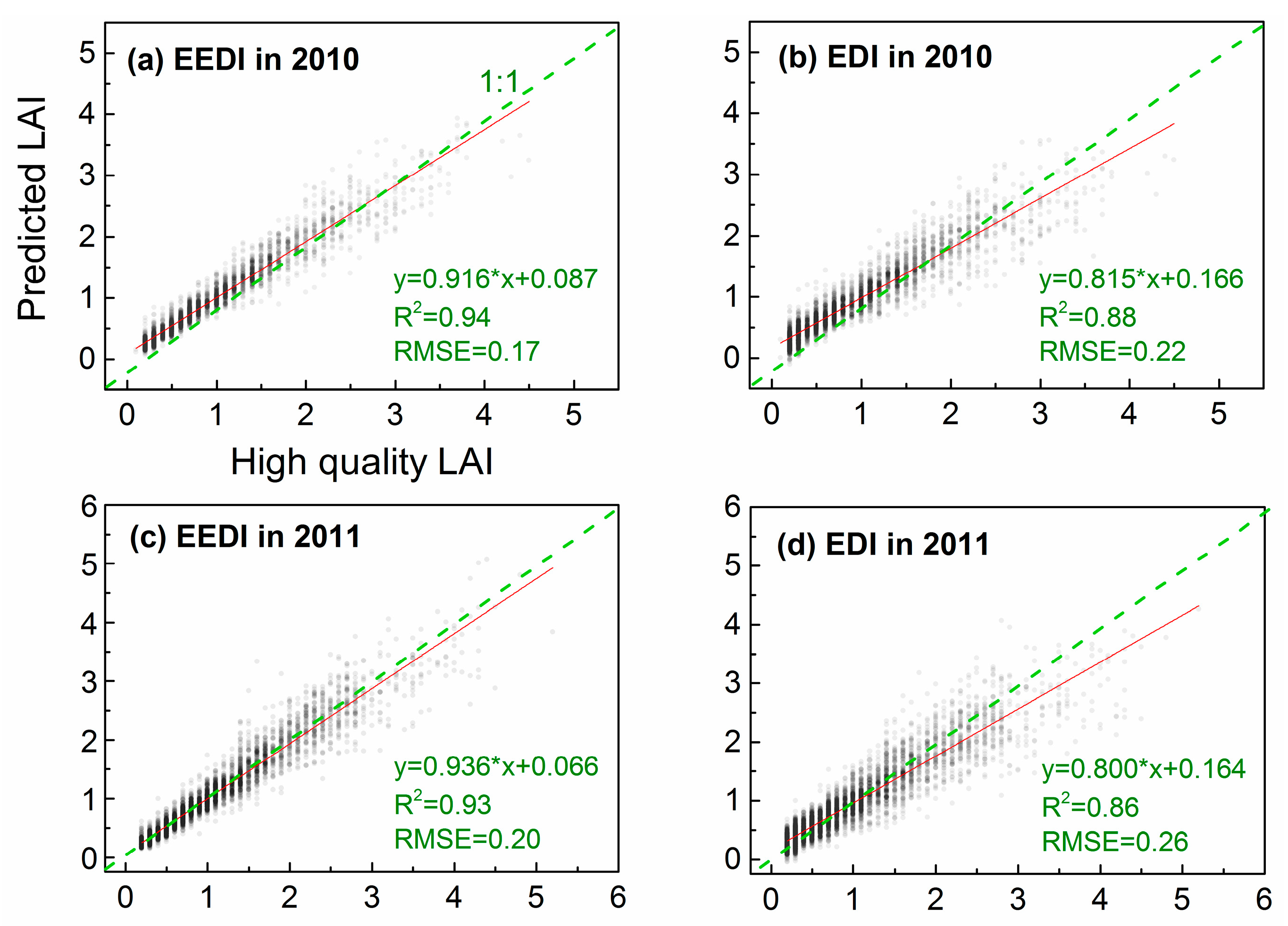
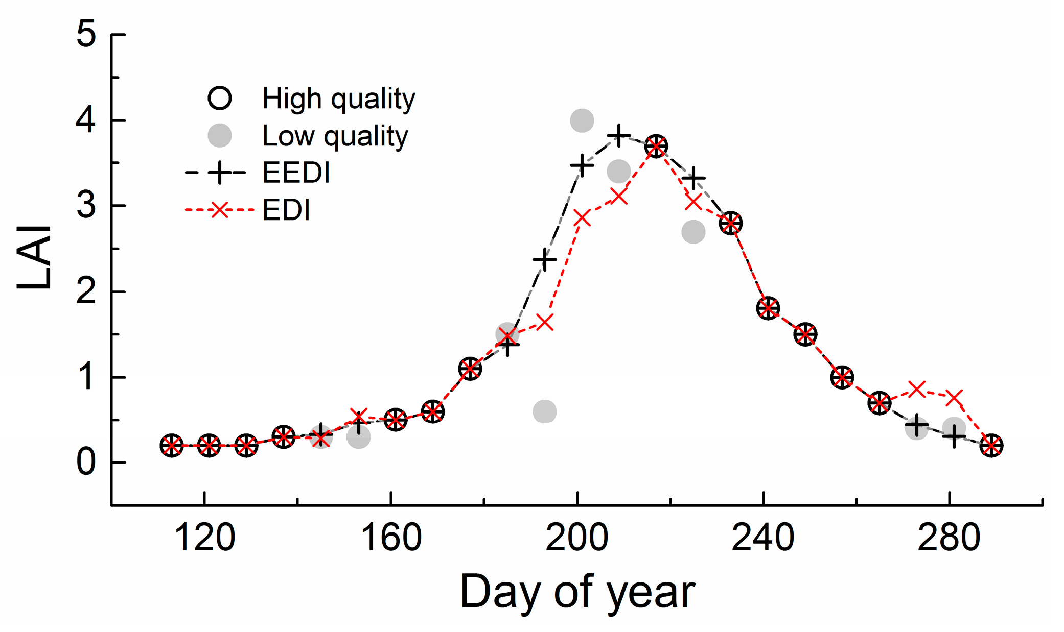
The overall accuracies of the two algorithms are provided in Figure 4. The EEDI algorithm achieved good performance in both dry (2010) and wet (2011) years with R2 > 0.9 and RMSE < 0.2. Furthermore, the distributions of the points in Figure 4a,c were close to the 1:1 line. The EDI algorithm showed lower performance as indicated by all of the four metrics. In addition, the RMSE values were higher in 2011 than that in 2010 for both the two algorithms. This may be due to the higher mean LAI value in 2011. Figure 5 provides an example of the gap filled LAI time series of a pixel in 2011 by the two algorithms.
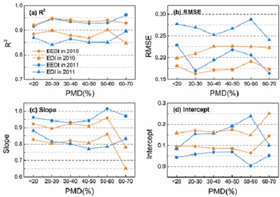
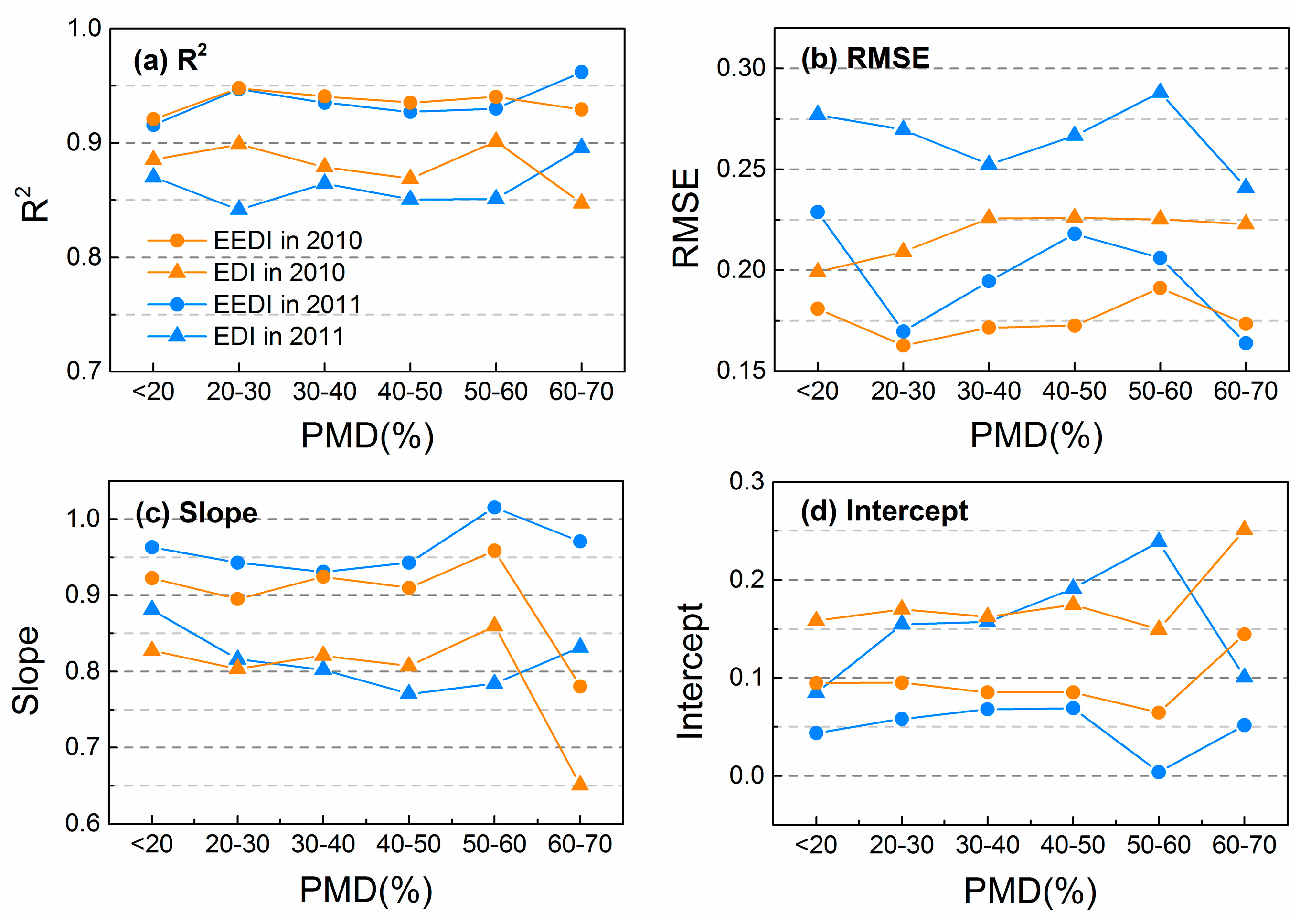
Figure 6 represents the effects of PMD on the interpolation performance. For the EEDI algorithm, all PMD levels showed high accuracies except for the PMD 60–70% in 2010 (slope < 0.8, intercept > 0.1). The linear functions for most PMD levels were close to the 1:1 line with 0.9 < slope < 1.1 and 0 < intercept < 0.1. For the EDI algorithm, no PMD level showed higher R2 or lower RMSE than that of the EEDI algorithm. Most of the corresponding regression functions had slope < 0.9 and intercept > 0.1. Furthermore, we found that the accuracies of low PMD levels were not necessarily higher than that of high PMD levels for both of the two algorithms. This may be related to the heterogeneity pattern of the grasslands in the test area.
3.3. Effects of SMD on Interpolation
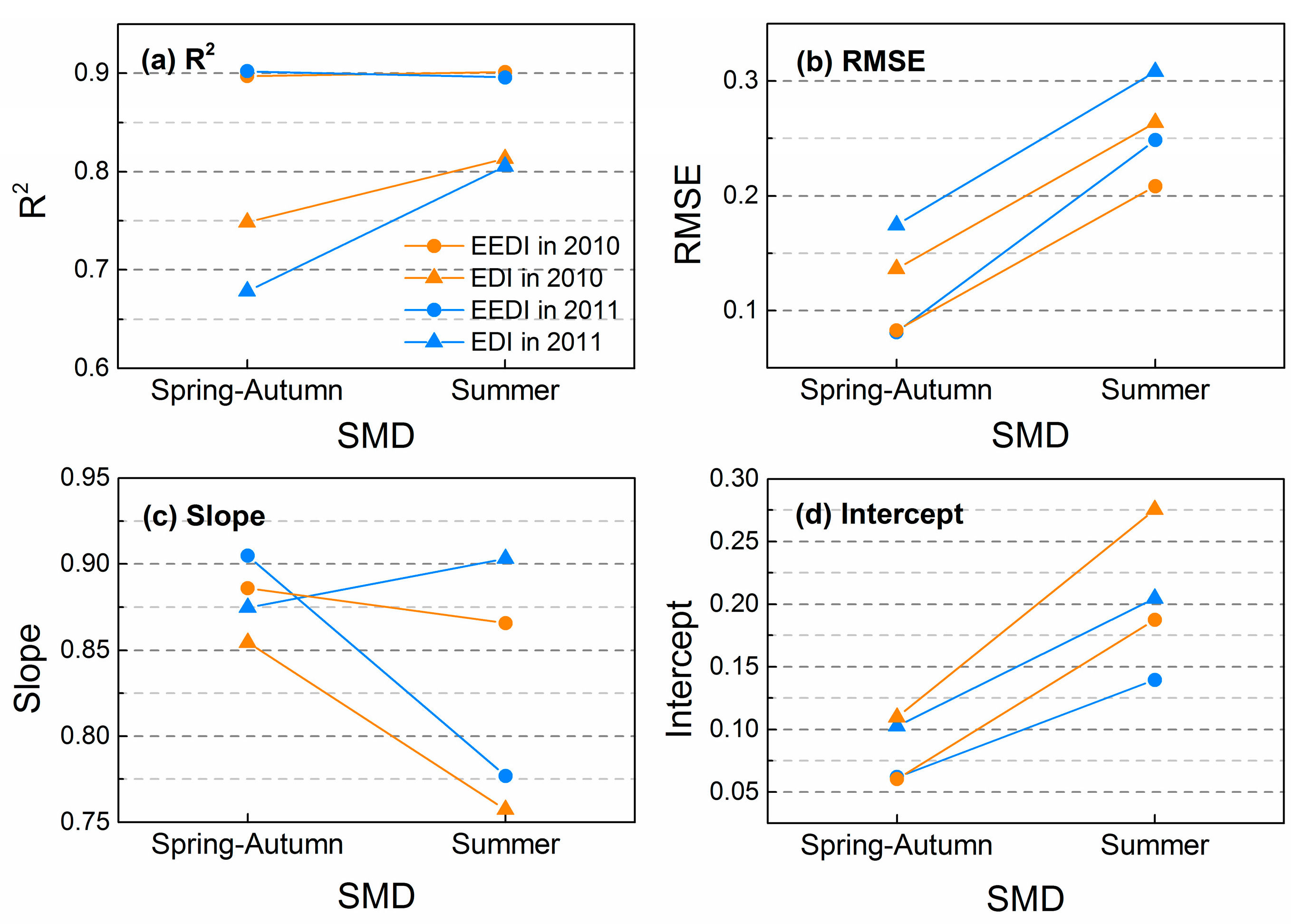
We also compared the accuracies of the two algorithms from the aspect of seasons. We separated the validation dataset into two parts based on the dates of the validation data: spring–autumn (day of year 113–151, 244–289) and summer (day of year 152–243). Spring and autumn are evaluated together because grasslands generally show inverse but similar behaviors in the two seasons. The EEDI algorithm achieved high R2 in both spring–autumn and summer (Figure 7). In contrast, the EDI algorithm did not perform well especially in spring–autumn with much lower R2 than the EEDI algorithm. Here, we found a significant advantage of the EEDI algorithm, i.e., predicting missing data in spring and autumn, which is challenging for the EDI algorithm. In spring and autumn, the heterogeneous grasslands are likely to exhibit more significantly different phenological behaviors than that in summer. A regional average curve could not explain this heterogeneity and, therefore, results in high uncertainties in predicting LAI value in spring and autumn. This promotion is expected to be helpful to more accurately extract the start and end of growing season with LAI data.
4. Discussion
To address the uncertainties in interpolating missing data of satellite-derived LAI time series caused by the construction and selection of reference time series in heterogeneous grasslands, we developed an improved algorithm that uses more flexible spatial-temporal constraints information. The algorithm achieved high performance in both dry and wet years in the test area, which shows typical heterogeneous landscapes.
The major differences between our algorithm and the previous algorithms [23,25] include: (1) multiple reference LAI time series are used, and they are missing data-dependent. There is no mandatory requirement of a complete LAI time series as reference; (2) only very strong phenological links are selected to provide more reliable references to more accurately predict missing data, and (3) an iterative process is employed. The iterative process is critical to update spatial-temporal constraint information for an LAI time series, particularly time series with high PMD. Benefiting from the above improvements, our algorithm showed advantages in predicting missing data for all PMD levels.
Although the EEDI algorithm showed relatively high overall accuracies with R2 > 0.9 and RMSE < 0.2, efforts are still needed to further reduce the uncertainties. In general, the uncertainties of the interpolation may be mainly derived from (1) the remaining low quality LAI in the input data and (2) the used phenological links. Although we performed a quality check to remove low quality data with the help from the quality flags and some empirical criteria, there may still remain some low level noise mainly derived from high aerosol and the LAI retrieval method. Stricter criteria are needed to provide higher quality inputs. Some statistical approaches in temporal or frequency domain, for example the wavelet analysis and the best index slope extraction algorithm (BISE) [36], may be useful to further check noise before interpolation. The phenological links used in our algorithm are linear functions with R2 > 0.95. However, it is difficult for the time series of some pixels to up to a strict linear relation. In [25], the quadratic polynomial function was used to construct phenological links. Nevertheless, using only nonlinear function can also introduce uncertainties when the link is approximately linear. Combining both linear and nonlinear links is one possible way to construct more reliable spatial-temporal constraints. On the other hand, although the iterative process is important for time series with high PMD, more iterative times may also generate uncertainties in estimating phenological links. In the test area, most time series were completely interpolated after two to three iterations. The interpolation accuracies suggest that these iterative times are acceptable. Instead of generating spurious results, it is reasonable to discard the incomplete time series after three iterations or more than 90% time series have been completed within a region. Furthermore, the phenological links are constructed using a temporal window covering the whole growing period to obtain more stable regression. Some local variations in the time series may not be fully considered because each point in the time series has equal contribution to the regression. Further studies may adjust temporal window or introduce weight to address this issue [37]. Using reference information from multiyear data has been suggested in several studies [24,25,38]. Its usefulness for semi-arid grasslands that show high interannual variability is currently not clear and needs to be investigated.
A complete LAI time series generated by any interpolation algorithm may contain low level noise caused by the input data and the algorithm. In [27], the Savitzky–Golay filter [7] was applied to the addressed MODIS LAI time series by the temporal-spatial filter interpolation method [24]. We recommend this two-step strategy to obtain smoother LAI time series, which is required for the extraction of vegetation phenology.
The algorithm is demonstrated to be effective to produce gap filled MODIS LAI time series for grasslands with high within-ecosystem heterogeneity. It should be emphasized that the algorithm was only designed for pixel-level heterogeneous landscape. Subpixel-level heterogeneity was not considered. Although the algorithm is developed especially for grasslands, it may also be applicable to other heterogeneous landscapes that show obvious seasonality with appropriate adjustments.
5. Conclusions
An algorithm for interpolating missing data in LAI time series for heterogeneous grasslands is presented based on spatial-temporal constraints. Considering the difficulty in constructing an ideal reference LAI time series for a pixel in such ecosystems, we developed a flexible strategy to select reference LAI time series and fill the gaps with an iteration process based on all available time series showing very strong phenological links with the target pixel. The interpolation results of our algorithm agreed with the validation data. Compared with the algorithm using a regional average reference time series, our algorithm can more accurately predict missing LAI value for different seasons and proportions of missing data. Future efforts may focus on improving the interpolation accuracy by incorporating multiyear time series or nonlinear phenological links.
Acknowledgments
This work was supported by the National Natural Science Foundation of China (Grant No. 41571405) and Fundamental Research Funds for the Central Universities (Grant No. 2652016129). The MCD15A2H and MCD12Q1 datasets were acquired from the Level-1 & Atmosphere Archive and Distribution System (LAADS) Distributed Active Archive Center (DAAC), located in the Goddard Space Flight Center in Greenbelt, Maryland (https://ladsweb.nascom.nasa.gov/). We are grateful to the three reviewers and the academic editor for their constructive comments.
Author Contributions
C.D. and X.L. conceived and designed the experiments; C.D. performed the experiments and wrote the paper; C.D. and F.H. analyzed the data. All authors contributed to the preparation of the manuscript.
Conflicts of Interest
The authors declare no conflicts of interest.
References
- Chen, J.M.; Black, T.A. Defining leaf-area index for non-flat leaves. Plant Cell Environ. 1992, 15, 421–429. [Google Scholar] [CrossRef]
- Myneni, R.B.; Hoffman, S.; Knyazikhin, Y.; Privette, J.L.; Glassy, J.; Tian, Y.; Wang, Y.; Song, X.; Zhang, Y.; Smith, G.R.; et al. Global products of vegetation leaf area and fraction absorbed PAR from year one of MODIS data. Remote Sens. Environ. 2002, 83, 214–231. [Google Scholar] [CrossRef]
- Ganguly, S.; Schull, M.A.; Samanta, A.; Shabanov, N.V.; Milesi, C.; Nemani, R.R.; Knyazikhin, Y.; Myneni, R.B. Generating vegetation leaf area index earth system data record from multiple sensors. Part 1: Theory. Remote Sens. Environ. 2008, 112, 4333–4343. [Google Scholar] [CrossRef]
- Yang, W.; Shabanov, N.V.; Huang, D.; Wang, W.; Dickinson, R.E.; Nemani, R.R.; Knyazikhin, Y.; Myneni, R.B. Analysis of leaf area index products from combination of MODIS Terra and Aqua data. Remote Sens. Environ. 2006, 104, 297–312. [Google Scholar] [CrossRef]
- Stoeckli, R.; Rutishauser, T.; Baker, I.; Liniger, M.A.; Denning, A.S. A global reanalysis of vegetation phenology. J. Geophys. Res. 2011, 116, G03020. [Google Scholar] [CrossRef]
- Verger, A.; Filella, I.; Baret, F.; Penuelas, J. Vegetation baseline phenology from kilometric global LAI satellite products. Remote Sens. Environ. 2016, 178, 1–14. [Google Scholar] [CrossRef]
- Chen, J.; Jonsson, P.; Tamura, M.; Gu, Z.H.; Matsushita, B.; Eklundh, L. A simple method for reconstructing a high-quality NDVI time-series data set based on the Savitzky–Golay filter. Remote Sens. Environ. 2004, 91, 332–344. [Google Scholar] [CrossRef]
- Olsson, L.; Eklundh, L. Fourier-series for analysis of temporal sequences of satellite sensor imagery. Int. J. Remote Sens. 1994, 15, 3735–3741. [Google Scholar] [CrossRef]
- Roerink, G.J.; Menenti, M.; Verhoef, W. Reconstructing cloudfree NDVI composites using Fourier analysis of time series. Int. J. Remote Sens. 2000, 21, 1911–1917. [Google Scholar] [CrossRef]
- Moody, A.; Johnson, D.M. Land-surface phenologies from AVHRR using the discrete Fourier transform. Remote Sens. Environ. 2001, 75, 305–323. [Google Scholar] [CrossRef]
- Yang, G.; Shen, H.; Zhang, L.; He, Z.; Li, X. A moving weighted harmonic analysis method for reconstructing high-quality SPOT VEGETATION NDVI time-series data. IEEE Trans. Geosci. Remote Sens. 2015, 53, 6008–6021. [Google Scholar] [CrossRef]
- Sakamoto, T.; Yokozawa, M.; Toritani, H.; Shibayama, M.; Ishitsuka, N.; Ohno, H. A crop phenology detection method using time-series MODIS data. Remote Sens. Environ. 2005, 96, 366–374. [Google Scholar] [CrossRef]
- Lu, X.; Liu, R.; Liu, J.; Liang, S. Removal of noise by wavelet method to generate high quality temporal data of terrestrial MODIS products. Photogramm. Eng. Remote Sens. 2007, 73, 1129–1139. [Google Scholar] [CrossRef]
- Qiu, B.; Feng, M.; Tang, Z. A simple smoother based on continuous wavelet transform: Comparative evaluation based on the fidelity, smoothness and efficiency in phenological estimation. Int. J. Appl. Earth Obs. Geoinf. 2016, 47, 91–101. [Google Scholar] [CrossRef]
- Jonsson, P.; Eklundh, L. Seasonality extraction by function fitting to time-series of satellite sensor data. IEEE Trans. Geosci. Remote Sens. 2002, 40, 1824–1832. [Google Scholar] [CrossRef]
- Zhang, X.; Friedl, M.A.; Schaaf, C.B.; Strahler, A.H.; Hodges, J.C.F.; Gao, F.; Reed, B.C.; Huete, A. Monitoring vegetation phenology using MODIS. Remote Sens. Environ. 2003, 84, 471–475. [Google Scholar] [CrossRef]
- Hird, J.N.; McDermid, G.J. Noise reduction of NDVI time series: An empirical comparison of selected techniques. Remote Sens. Environ. 2009, 113, 248–258. [Google Scholar] [CrossRef]
- Atkinson, P.M.; Jeganathan, C.; Dash, J.; Atzberger, C. Inter-comparison of four models for smoothing satellite sensor time-series data to estimate vegetation phenology. Remote Sens. Environ. 2012, 123, 400–417. [Google Scholar] [CrossRef]
- Kandasamy, S.; Baret, F.; Verger, A.; Neveux, P.; Weiss, M. A comparison of methods for smoothing and gap filling time series of remote sensing observations—Application to MODIS LAI products. Biogeosciences 2013, 10, 4055–4071. [Google Scholar] [CrossRef]
- Kandasamy, S.; Fernandes, R. An approach for evaluating the impact of gaps and measurement errors on satellite land surface phenology algorithms: Application to 20 year NOAA AVHRR data over Canada. Remote Sens. Environ. 2015, 164, 114–129. [Google Scholar] [CrossRef]
- Geng, L.; Ma, M.; Wang, X.; Yu, W.; Jia, S.; Wang, H. Comparison of eight techniques for reconstructing multi-satellite sensor time-series NDVI data sets in the Heihe river basin, China. Remote Sens. 2014, 6, 2024–2049. [Google Scholar] [CrossRef]
- Zhou, J.; Jia, L.; Menenti, M.; Gorte, B. On the performance of remote sensing time series reconstruction methods—A spatial comparison. Remote Sens. Environ. 2016, 187, 367–384. [Google Scholar] [CrossRef]
- Moody, E.G.; King, M.D.; Platnick, S.; Schaaf, C.B.; Gao, F. Spatially complete global spectral surface albedos: Value-added datasets derived from Terra MODIS land products. IEEE Trans. Geosci. Remote Sens. 2005, 43, 144–158. [Google Scholar] [CrossRef]
- Fang, H.; Liang, S.; Townshend, J.R.; Dickinson, R.E. Spatially and temporally continuous LAI data sets based on an integrated filtering method: Examples from North America. Remote Sens. Environ. 2008, 112, 75–93. [Google Scholar] [CrossRef]
- Gao, F.; Morisette, J.T.; Wolfe, R.E.; Ederer, G.; Pedelty, J.; Masuoka, E.; Myneni, R.; Tan, B.; Nightingale, J. An algorithm to produce temporally and spatially continuous MODIS-LAI time series. IEEE Geosci. Remote Sens. Lett. 2008, 5, 60–64. [Google Scholar] [CrossRef]
- Borak, J.S.; Jasinski, M.F. Effective interpolation of incomplete satellite-derived leaf-area index time series for the continental United States. Agric. For. Meteorol. 2009, 149, 320–332. [Google Scholar] [CrossRef]
- Yuan, H.; Dai, Y.; Xiao, Z.; Ji, D.; Shangguan, W. Reprocessing the MODIS leaf area index products for land surface and climate modelling. Remote Sens. Environ. 2011, 115, 1171–1187. [Google Scholar] [CrossRef]
- Vuolo, F.; Ng, W.-T.; Atzberger, C. Smoothing and gap-filling of high resolution multi-spectral time series: Example of Landsat data. Int. J. Appl. Earth Obs. Geoinf. 2017, 57, 202–213. [Google Scholar] [CrossRef]
- Elmore, A.J.; Guinn, S.M.; Minsley, B.J.; Richardson, A.D. Landscape controls on the timing of spring, autumn, and growing season length in mid-Atlantic forests. Glob. Chang. Biol. 2012, 18, 656–674. [Google Scholar] [CrossRef]
- Klosterman, S.T.; Hufkens, K.; Gray, J.M.; Melaas, E.; Sonnentag, O.; Lavine, I.; Mitchell, L.; Norman, R.; Friedl, M.A.; Richardson, A.D. Evaluating remote sensing of deciduous forest phenology at multiple spatial scales using PhenoCam imagery. Biogeosciences 2014, 11, 4305–4320. [Google Scholar] [CrossRef] [Green Version]
- De Beurs, K.M.; Henebry, G.M. Spatio-temporal statistical methods for modeling land surface phenology. In Phenological Research: Methods for Environmental and Climate Change Analysis; Hudson, I.L., Keatley, M.R., Eds.; Springer: Dordrecht, The Netherlands, 2010; pp. 177–208. [Google Scholar]
- Zheng, H.Y.; Li, J.D. Saline Plants in Songnen Plain and Restoration of Alkaline-Saline Grass; Science Press: Beijing, China, 1999; pp. 179–206. [Google Scholar]
- Shang, Z.B.; Gao, Q.; Dong, M. Impacts of grazing on the alkalinized-salinized meadow steppe ecosystem in the Songnen plain, China—A simulation study. Plant Soil 2003, 249, 237–251. [Google Scholar] [CrossRef]
- Bai, L.; Wang, C.; Zang, S.; Zhang, Y.; Hao, Q.; Wu, Y. Remote sensing of soil alkalinity and salinity in the Wuyu’er-Shuangyang river basin, northeast China. Remote Sens. 2016, 8, 163. [Google Scholar] [CrossRef]
- Knyazikhin, Y.; Martonchik, J.V.; Myneni, R.B.; Diner, D.J.; Running, S.W. Synergistic algorithm for estimating vegetation canopy leaf area index and fraction of absorbed photosynthetically active radiation from MODIS and MISR data. J. Geophys. Res. Atmos. 1998, 103, 32257–32275. [Google Scholar] [CrossRef]
- Viovy, N.; Arino, O.; Belward, A.S. The best index slope extraction (BISE)—A method for reducing noise in NDVI time-series. Int. J. Remote Sens. 1992, 13, 1585–1590. [Google Scholar] [CrossRef]
- Verger, A.; Baret, F.; Weiss, M.; Kandasamy, S.; Vermote, E. The CACAO method for smoothing, gap filling, and characterizing seasonal anomalies in satellite time series. IEEE Trans. Geosci. Remote Sens. 2013, 51, 1963–1972. [Google Scholar] [CrossRef]
- Chen, J.; Rao, Y.; Shen, M.; Wang, C.; Zhou, Y.; Ma, L.; Tang, Y.; Yang, X. A simple method for detecting phenological change from time series of vegetation index. IEEE Trans. Geosci. Remote Sens. 2016, 54, 3436–3449. [Google Scholar] [CrossRef]
Figure 1.
Land cover types (a) and growing season mean leaf area index (LAI) of grasslands (b) for the test area in 2011.
Figure 1.
Land cover types (a) and growing season mean leaf area index (LAI) of grasslands (b) for the test area in 2011.

Figure 2.
Flow chart of the Enhanced Ecosystem-Dependent Interpolation (EEDI) algorithm.

Figure 3.
Statistics of the number of point in LAI time series during the iterative process.

Figure 4.
Overall interpolation accuracies of the EEDI and EDI algorithms.

Figure 5.
The original and interpolated LAI time series of a pixel in 2011.

Figure 6.
Interpolation accuracies of the EEDI and EDI algorithms for different proportions of missing data (PMD) quantified by (a) coefficient of determination R2, (b) root mean square error (RMSE), (c) slope, and (d) intercept.
Figure 6.
Interpolation accuracies of the EEDI and EDI algorithms for different proportions of missing data (PMD) quantified by (a) coefficient of determination R2, (b) root mean square error (RMSE), (c) slope, and (d) intercept.

Figure 7.
Interpolation accuracies of the EEDI and EDI algorithms for different seasons of missing data (SMD) quantified by (a) R2, (b) RMSE, (c) slope, and (d) intercept.
Figure 7.
Interpolation accuracies of the EEDI and EDI algorithms for different seasons of missing data (SMD) quantified by (a) R2, (b) RMSE, (c) slope, and (d) intercept.


Table 1.
Items of quality flags for identifying high quality data.
| Items | Flags of High Quality Data 1 |
|---|---|
| Five-level confidence score | Main method used, best result possible (no saturation); Main method used with saturation |
| Cloud | Significant clouds not present (clear) |
| Cloud shadow | No cloud shadow detected |
| Cirrus | No cirrus detected |
| Snow/Ice | No snow/ice detected |
1 For detailed description on the quality flags, please refer to the user’s guide of Moderate Resolution Imaging Spectroradiometer (MODIS) leaf area index (LAI) product (https://lpdaac.usgs.gov/sites/default/files/public/MODIS/docs/MODIS-LAI-FPAR-User-Guide.pdf).
© 2017 by the authors. Licensee MDPI, Basel, Switzerland. This article is an open access article distributed under the terms and conditions of the Creative Commons Attribution (CC BY) license (http://creativecommons.org/licenses/by/4.0/).
Share and Cite
MDPI and ACS Style
Ding, C.; Liu, X.; Huang, F. Temporal Interpolation of Satellite-Derived Leaf Area Index Time Series by Introducing Spatial-Temporal Constraints for Heterogeneous Grasslands. Remote Sens. 2017, 9, 968. https://doi.org/10.3390/rs9090968
AMA Style
Ding C, Liu X, Huang F. Temporal Interpolation of Satellite-Derived Leaf Area Index Time Series by Introducing Spatial-Temporal Constraints for Heterogeneous Grasslands. Remote Sensing. 2017; 9(9):968. https://doi.org/10.3390/rs9090968
Chicago/Turabian StyleDing, Chao, Xiangnan Liu, and Fang Huang. 2017. "Temporal Interpolation of Satellite-Derived Leaf Area Index Time Series by Introducing Spatial-Temporal Constraints for Heterogeneous Grasslands" Remote Sensing 9, no. 9: 968. https://doi.org/10.3390/rs9090968
Note that from the first issue of 2016, this journal uses article numbers instead of page numbers. See further details here.