Calibration of the Water Cloud Model at C-Band for Winter Crop Fields and Grasslands


1
Institut National de Recherche en Sciences et Technologies Pour l’Environnement et l’Agriculture (IRSTEA), UMR TETIS, 500 rue François Breton, 34093 Montpellier CEDEX 5, France
2
French National Centre for Scientific Research (CESBIO), 18 av. Edouard Belin, bpi 2801, 31401 Toulouse CEDEX 9, France
3
Institut National Agronomique de Tunis, Université de Carthage, Tunis, Tunisia
*
Author to whom correspondence should be addressed.
Remote Sens. 2017, 9(9), 969; https://doi.org/10.3390/rs9090969
Submission received: 21 August 2017
/
Revised: 12 September 2017
/
Accepted: 18 September 2017
/
Published: 20 September 2017
(This article belongs to the Section Remote Sensing in Agriculture and Vegetation)
Abstract
:In a perspective to develop an inversion approach for estimating surface soil moisture of crop fields from Sentinel-1/2 data (radar and optical sensors), the Water Cloud Model (WCM) was calibrated from C-band Synthetic Aperture Radar (SAR) data and Normalized Difference Vegetation Index (NDVI) values collected over crops fields and grasslands. The soil contribution that depends on soil moisture and surface roughness (in addition to SAR instrumental parameters) was simulated using the physical backscattering model IEM (Integral Equation Model). The vegetation descriptor used in the WCM is the NDVI because it can be directly calculated from optical images. A large dataset consisting of radar backscattered signal in Vertical transmit and Vertical receive (VV) and Vertical transmit and Horizontal receive (VH) polarizations with wide range of incidence angle, soil moisture, surface roughness, and NDVI-values was used. It was collected over two agricultural study sites. Results show that the soil contribution to the total radar backscattered signal is lower in VH than in VV because VH is more sensitive to vegetation cover. Thus, the use of VH alone or in addition to VV for retrieving the soil moisture is not advantageous in presence of well-developed vegetation cover.
1. Introduction
The new C-band radar satellites Sentinel-1A (launched on 3 April 2014) and Sentinel-1B (launched on 22 April 2016), in addition to the optical satellites Sentinel-2A and Sentinel-2B (launched on 23 June 2015 and 7 March 2017, respectively), provide free and open access data for the whole globe with high spatial and temporal resolutions (six days with Sentinel-1 satellites and five days with Sentinel-2 satellites at 10 m spatial resolution). This availability of both Sentinel-1 and Sentinel-2 satellites allows the coupling of SAR (Synthetic Aperture Radar) and optical data for operational soil moisture mapping at field scale.
SAR remote sensing was widely used to estimate the surface soil moisture in agricultural areas (e.g., [1,2,3,4,5,6,7,8,9]). Over bare soil, the estimation of soil moisture is performed using either a physical (e.g., the Integral Equation Model [10] or statistical (e.g., Baghdadi [11], Dubois [12], and Oh models [13]), with an accuracy better than 6 vol % [3,14,15]. As soils of agricultural areas are covered for a long period of the year by vegetation, an approach that considers the effects of vegetation on the backscattered radar signal for estimating the soil moisture is therefore necessary. The presence of vegetation cover makes soil moisture retrieval from SAR data more complicated because the soil’s contribution is attenuated by the vegetation. So, the estimation of soil moisture on agricultural areas with a good accuracy requires the use of a well calibrated radar backscattering model that takes into account both vegetation and soil contributions.
Most studies used the Water Cloud Model (WCM) in an inversion scheme for soil moisture estimation over areas with vegetation cover. The two terms, direct vegetation contribution and attenuation, are computed using one vegetation parameter representing the vegetation effect. This vegetation parameter could be estimated from optical data. Therefore, the best way for soil moisture retrieval over areas covered by vegetation is to combine SAR and optical data [4,5,6,16,17,18,19,20]. Currently, the high temporal repetitiveness of Sentinel-1 and Sentinel-2 data makes it possible to combine SAR and optical data for soil moisture monitoring at time scale close to user requirements (weekly to daily depending on the applications).
In this study, the Water Cloud Model combined with the Integral Equation Model was parameterized using real data composed of C-band radar backscattered signal, NDVI, soil moisture, and surface roughness values. In the Water Cloud Model, the NDVI was used as the vegetation descriptor because it is easier to derive NDVI from optical data than the other vegetation descriptors, such as Leaf Area Index (LAI), vegetation water content (VWC), biomass, vegetation height, fraction of absorbed photosynthetically active radiation (FAPAR), or the fractional vegetation cover (FCOVER). Several studies showed that the correlation between the NDVI and the vegetation parameters (LAI, VWC, biomass, etc.) is strong when the NDVI is less than 0.7–0.8 [21,22,23]. Beyond 0.7–0.8, the NDVI saturates and does not vary with the increase of the vegetation parameters. For example, the logarithmic relationship observed between NDVI and LAI saturates when the LAI exceeded 2–3 m2/m2 [6,21,22,23].
The research presented in this paper aims mainly to prepare the combined use of the new Sentinel-1 SAR data with Sentinel-2 optical data for operational soil moisture mapping at field scale. The resulting parameterized WCM permits the evaluation of the potential of C-band SAR data combined with optical data to estimate soil moisture over agricultural areas. In this paper, Section 2 presents the study areas and the ground-truth in situ measurements. Section 3 presents the radar signal modeling. The results and discussion are provided in Section 4. Finally, Section 5 presents the main conclusions.
2. Dataset Description
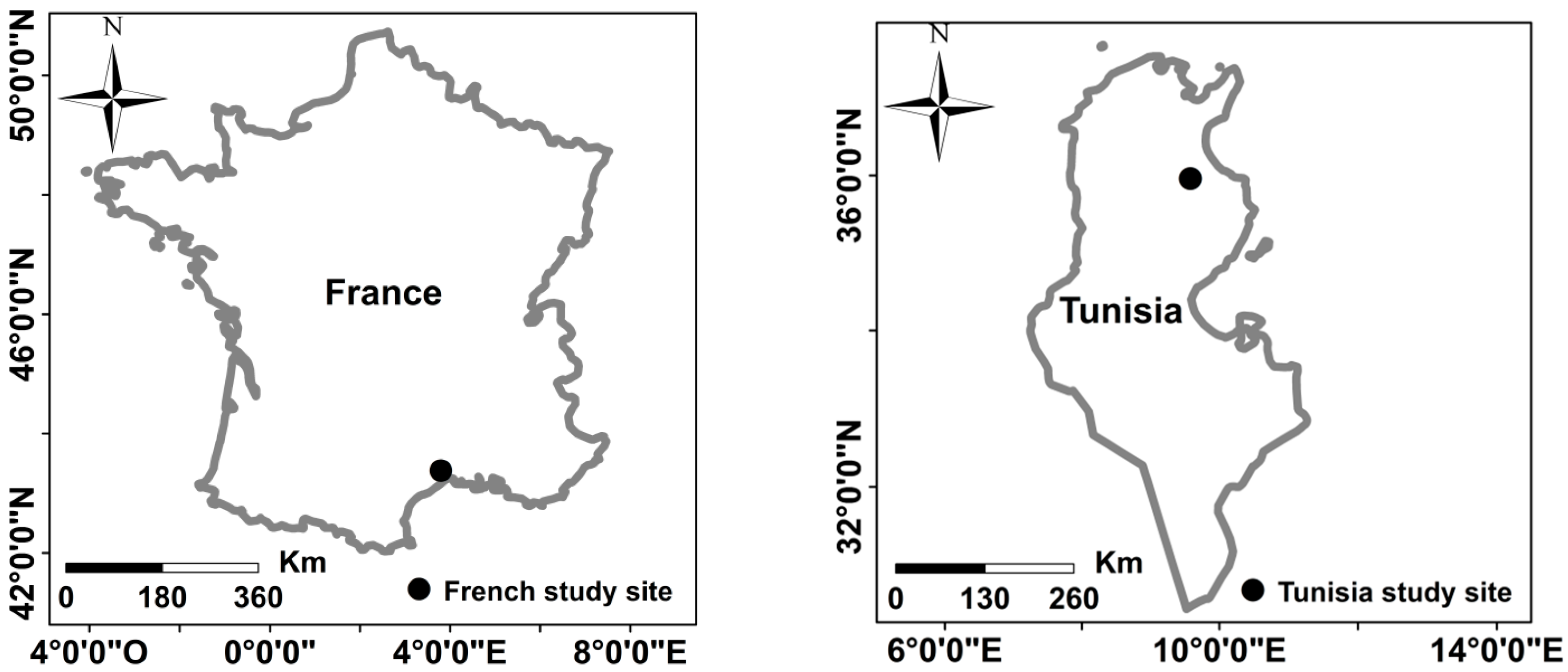
In the study presented, a wide experimental dataset was used, consisting of SAR and optical images as well as ground measurements of soil moisture and surface roughness collected over two agricultural study sites: one in France and one in Tunisia (Figure 1). SAR images were acquired by the C-band (radar wavelength about 6 cm) sensors ASAR and Sentinel-1, with incidence angles between 18° and 46°, and in VV and VH polarizations.
2.1. Study Sites
The French study site is located in southeastern France near Montpellier (43.38°52′–43°45′N, 03°47′−03°52′E, Figure 1). Relatively flat, it is composed mainly of forest, vineyard, grasslands, and agricultural fields (mainly wheat). This site is characterized by a Mediterranean climate with rainy season between mid-October and March and an average cumulative rainfall of approximately 750 mm. The average air temperature varies between 2.9 °C in December and 29.3 °C in July. The predominant soil texture of the agricultural fields is a loam.
The Tunisian study site is situated in the Kairouan plain (35°1′−35°55′N, 9°23′−10°17′E), in central Tunisia (Figure 1). The climate in this region is semi-arid, with an average annual rainfall of approximately 300 mm/year, characterized by a rainy season lasting from October to May, with the two rainiest months being October and March [15]. The temperature in Kairouan varies between 10.7 °C in January and 28.6 °C in August. The mean annual potential evapotranspiration (Penman) is close to 1600 mm. The study site consists mainly of agricultural fields (cereals) on flat landscape. Soil texture measurements showed a clay percentage between 2.4% and 53.1% and sand percentage between 4.4% and 84.3% [15].
2.2. Satellite Images
2.2.1. SAR Images
Twenty-five Sentinel-1 images were acquired between September 2016 and May 2017 (Table 1) over the French study site at incidence angle close to 39°, and in VV and VH polarizations. These images were acquired with a spatial resolution of 10 m.
Seven ASAR and 5 Sentinel-1 images were acquired over the Kairouan plain respectively between 2009 and 2012, and between 2015 and 2017. For ASAR images, the radar incidence angle varies between 18° and 40°, with VV and HH polarizations. Sentinel-1 images were acquired at incidence angle near to 39° with VV and VH polarizations.
The radiometric calibration and the orthorectification of the SAR images was carried out using algorithms developed by the European Space Agency (http://step.esa.int/main/toolboxes/snap). The radiometric calibration converts the digital number value to radar backscattering coefficients. In addition, our ortho-rectified images have pixel dimension of 10 m × 10 m.
2.2.2. Optical Images
At dates very close to the SAR images (less than 2 weeks), 11 free cloud Sentinel-2 images were acquired over the French site, and 12 Landsat images were acquired over the Tunisian site. The optical images corrected for atmospheric effects and orthorectified were used to calculate the NDVI. As the dates of the optical images were different from the SAR acquisition dates, the NDVI for each SAR acquisition date was estimated using a linear interpolation of the two NDVI-values calculated from optical images with acquisition dates preceding and succeeding the SAR image.
The NDVI-values ranged between 0.13 and 0.92 for the French site and between 0.08 and 0.86 for the Tunisia site.
2.3. In Situ Measurements
Simultaneously with the SAR acquisitions, in situ measurements of soil moisture and surface roughness were collected on several reference fields (cereals in Tunisia, cereals and grasslands in France). The size of the reference fields is in the range of 2 to 9 ha. Moisture measurements (mv) were made within a 2-h window around the SAR overpass time. Between 20 and 30 volumetric soil moisture measurements were performed in the first top layer (5 cm depth) for each reference field using calibrated TDR (Time Domain Reflectometry) probes. The mean volumetric soil moisture was then calculated for each reference field and each date. The soil moisture on the reference fields ranged between 7.0 and 36.3 vol % for the French site and between 4.0 and 39.65 vol % for the Tunisia site.
The soil roughness measurements made on the reference fields use 1 m long pin profiler with a resolution of 2 cm. Ten roughness profiles (five parallel and five perpendicular to the tillage row direction) were made in each reference field using a 1 m long needle-profilometer and a sampling interval of 2 cm. From these roughness profiles, the root mean square surface height (Hrms) were then calculated for each reference field using the mean of all autocorrelation functions acquired for each reference field. The rms surface height ranged between 0.8 cm and 4.0 cm for the reference fields in the French site (mainly wheat and grasslands) and between 0.7 cm and 4.6 cm for the reference fields (cereals) in the Tunisian site.
Finally, our dataset contains in situ measurements (mv and Hrms) and satellite information (mean of radar incidence angle, radar backscattered signals and NDVI). In the dataset, each of these latest data is associated to a SAR acquisition date. The mean of incidence angle, radar backscattered signals and NDVI were calculated by averaging for each reference field the values of all pixels within the reference field.
The dataset was divided into two sub-datasets. The first sub-dataset (training dataset) combining data on Tunisia site was used to fit the WCM (ASAR and Sentinel-1 data). The second (validation dataset) contains only data acquired on the French site (Sentinel-1 data) was used to validate the agreement between the radar signal of the fitted WCM and the radar backscattered signal of SAR images.
WCM was calibrated and validated in VV and VH. In the perspective of using Sentinel-1 data for estimating soil moisture, the WCM validated only in VV and VH is sufficient because these two polarizations correspond to the standard acquisition mode of Sentinel-1.
3. Radar Signal Modeling
In this study, the Water Cloud model (WCM) developed by [24], was used to model the radar backscattered signal in agricultural environments as a function of soil and vegetation parameters. This semi-empirical model is widely used because it can be easily performed in an inversion scheme to estimate soil moisture and vegetation parameters [5,6,25,26,27].
For a given polarization pq (pq = HH, VV or VH), the Water Cloud model defines the backscattered radar signal in linear scale (σ0tot) as the sum of the contribution from the vegetation (σ0veg), the soil (σ0soil) attenuated by the vegetation (T2σ0soil), and multiple soil-vegetation scatterings (often neglected).
where V1 and V2 are the vegetation’s descriptors. In most studies, authors use mainly vegetation water content [5,28], leaf area index [27,29], NDVI [4]. Recently, El Hajj et al. [4] obtained similar accuracy on soil moisture estimation over irrigated grassland using X-band SAR data when NDVI, LAI, FAPAR, and FCOVER were used in the WCM. In this paper, V1 = V2 = NDVI (NDVI values are calculated from the optical images); θ is the radar incidence angle (in); and are fitted parameters of the model that depend on the vegetation descriptor and the radar configuration; is the two way attenuation.
The soil contribution σ0soil depends on soil moisture and surface roughness (in addition to SAR instrumental parameters). It is simulated in this study using the physical backscattering model IEM [10] calibrated by Baghdadi et al. [30,31]. Baghdadi et al. [30,31] proposed an empirical calibration of the IEM model, in order to improve the determination of backscattering coefficients on bare agricultural soils. This calibration was based on a large experimental database composed of SAR images and ground measurements (soil moisture and roughness). The discrepancies between the IEM and satellite radar data were related both to the shape of the correlation function, and to the accuracy of the correlation length measurements. This calibration consisted in replacing the measured correlation length by a fitting parameter (Lopt) that depends on the rms surface height (Hrms) and the SAR parameters (radar incidence angle, and radar frequency).
At C-band, the fitting parameter Lopt was defined for each polarization as follows:
where θ is expressed in degrees, and Lopt and Hrms are expressed in cm. The formulations for Lopt were obtained with a Gaussian correlation function.
4. Results and Discussion
4.1. Water Cloud Model Parameterization
The WCM parameterization was performed using the training dataset (Table 1). WCM parameterization consists in fitting the model against ground measurements (Equations (1)–(3)). A and B parameters were estimated for VV and VH polarization by minimizing the sum of squares of the differences between the simulated and measured radar signal (Table 2). With A and B parameters, it becomes possible to simulate WCM components (σ0veg, T2, and σ0soil) and consequently the total backscattering coefficient (σ0tot) using NDVI, soil moisture and surface roughness as inputs in the WCM. Only data corresponding to NDVI values lower than 0.8 were used in the fitting and the validation of the WCM. It is due to the low sensitivity of NDVI to vegetation parameters (LAI, VWC…) in the case of high values of vegetation parameters [21,22,23].
4.2. Water Cloud Model Validation
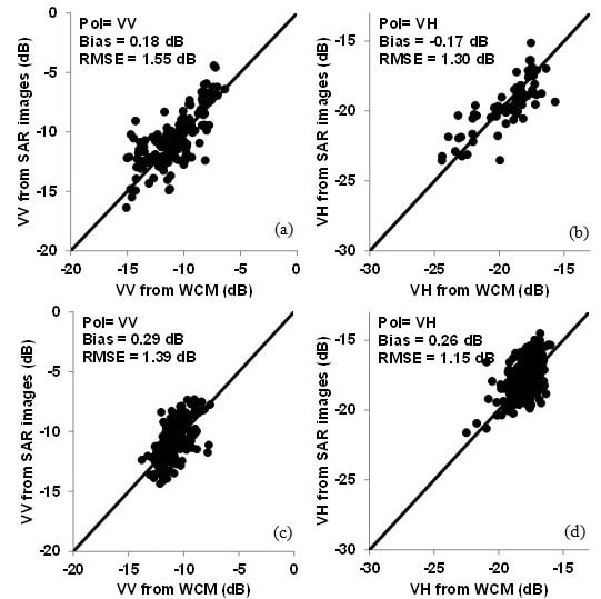
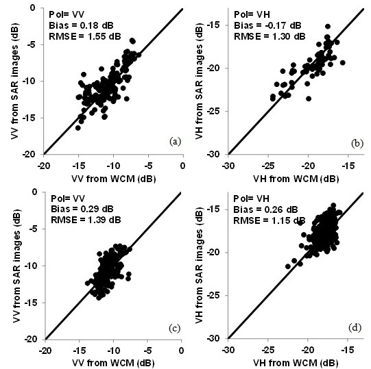
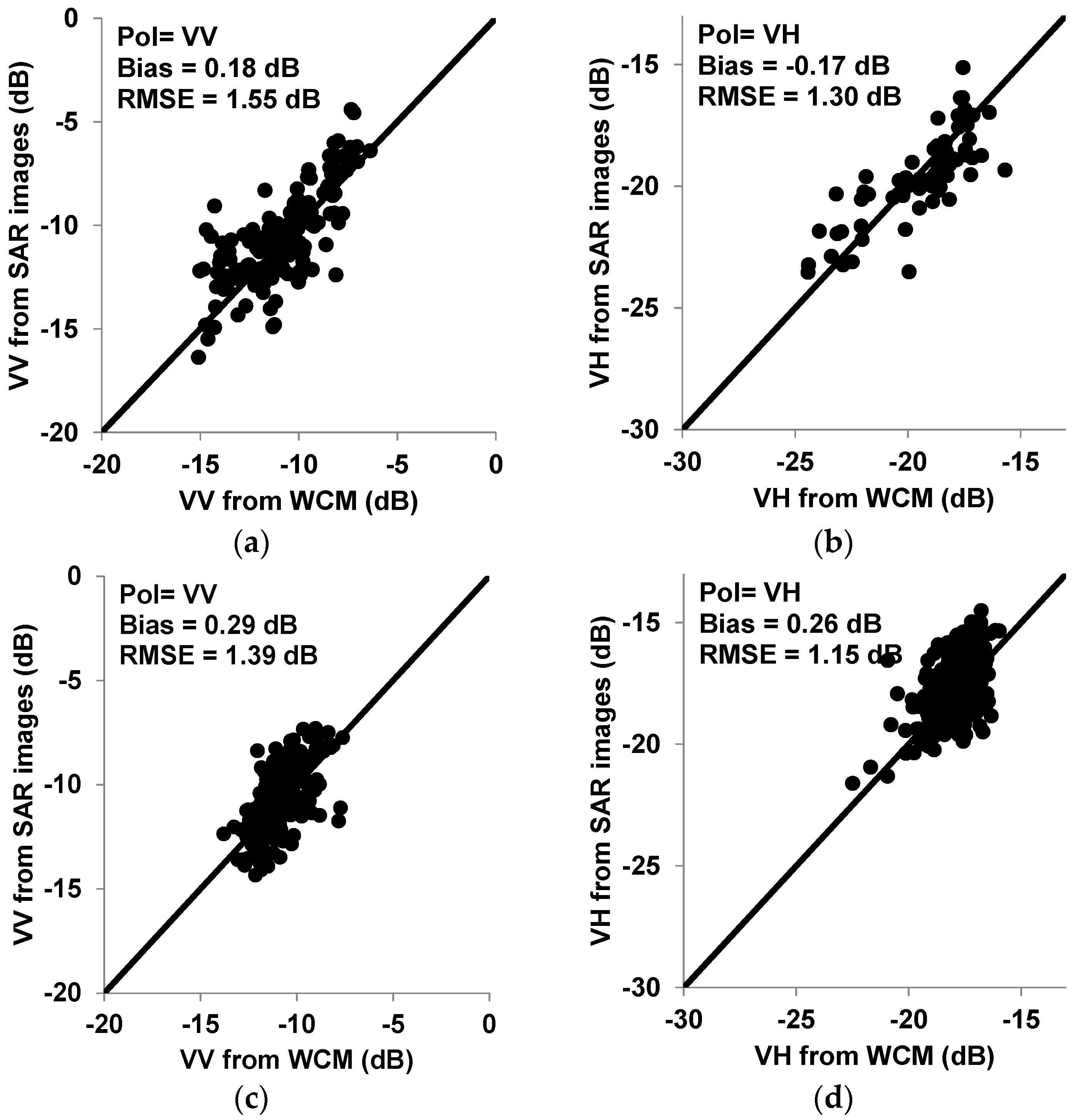
To validate the fitted WCM, a comparison was performed between the radar backscattering coefficients predicted by the parameterized WCM (using the training dataset) and the observed backscattering coefficients of the validation dataset (Table 1, Figure 2). Results showed that the fit of the WCM was similar in VV and VH polarizations (Table 2, Figure 2a,b). The correlation coefficient R2 is equal to 0.55 for VV and 0.63 for VH with RMSE (Root Mean Square Error) on the predicted backscattering coefficients of 1.55 dB in VV and 1.30 dB in VH. The RMSE obtained on the WCM predictions close to 1.5 dB are slightly higher than the Sentinel-1 precision [32,33]. Indeed, the radiometric accuracy for all measurement modes of Sentinel-1 is within 1 dB (3σ) and its sensitivity expressed by the noise equivalent sigma naught is −22 dB or higher [32].
The validation of the WCM using the validation dataset shows a RMSE on the predicted backscattering coefficients of 1.39 dB in VV and 1.15 dB in VH with a bias lower than 0.5 dB in both VV and VH (Figure 2c,d).
4.3. Behavior of Different Components of the WCM
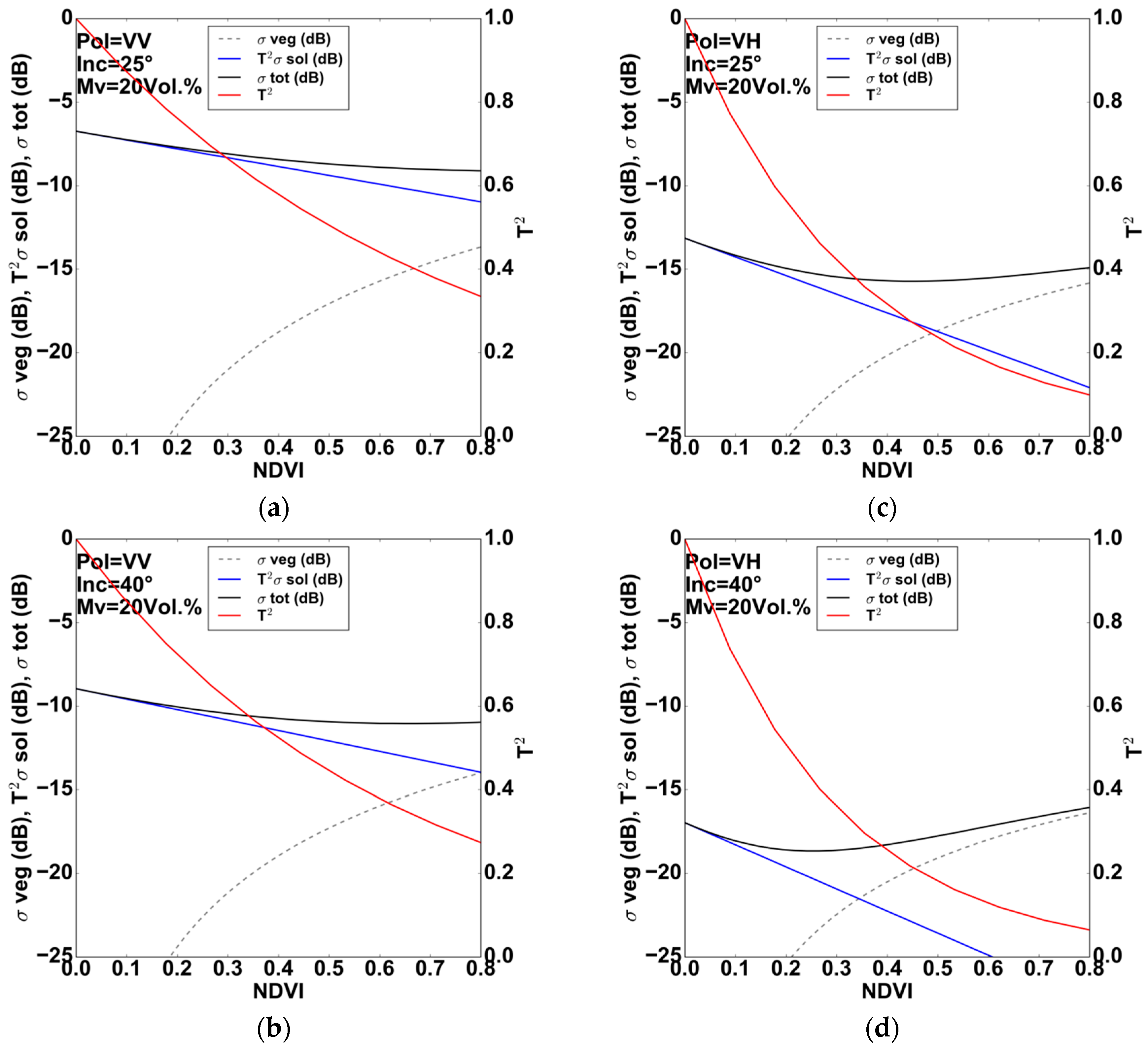
Modelling results obtained using the NDVI as the vegetation descriptor in the WCM will be presented and discussed in this section. The WCM components (T2σ0soil and σ0veg) were simulated for soil moisture (mv) between 5 and 35 vol % and NDVI-values between 0 and 0.8. These ranges of mv and NDVI values were used since they are the most encountered in agricultural environments. Radar incidence angles of 25° and 40° were chosen. The surface roughness used in these simulations corresponds to Hrms of 2 cm.
Figure 3 and Figure 4 show the modelled σ0veg, T2σ0soil and σ0tot in dB units as a function of mv using three different values of NDVI (0.3, 0.6, and 0.8), with 25° and 40° incidence angles, and Hrms = 2 cm. In addition, the modelled σ0veg, T2σ0soil and σ0tot were also plotted according to NDVI for mv values of 20 vol %, with 25° and 40° incidence angles, and Hrms = 2 cm (Figure 5).
Figure 3 shows that σ0tot in VV polarization are always sensitive to soil moisture (mv) even for high NDVI values (NDVI = 0.8). However, this sensitivity to soil moisture slightly decreases as the NDVI increases. As an example, for 25° incidence angle, this sensitivity decreases from 2.75 dB/% for NDVI = 0.3 to 1.65 dB/% for NDVI = 0.8 (σ0tot = S ln(mv) + b, with S is the sensitivity). Moreover, results also show that the sensitivity of σ0tot to soil moisture decreases slightly when the incidence angle increases. As an example, for NDVI = 0.8, the sensitivity of σ0tot to soil moisture decreases from 1.65 dB/% to 1.40 dB/% as the incidence angle increases from 25° to 40°. This is due to an increasing of vegetation attenuation effect and vegetation component.
The NDVI thresholds from which the soil’s contribution (T2σ0soil) is lower than the vegetation’s contribution (σ0veg) are given in Table 3. The threshold values in VV with 40° incidence angle are approximately 0.51 and 0.65 for soil moisture of 5 and 10 vol %, respectively. Results show that the soil contribution begins to dominate the vegetation contribution at 40° for mv-values higher than 10 vol %. The comparison between results obtained at 25° and 40° shows that the NDVI thresholds are higher at low incidence angle (25°) than at high incidence angle (40°) where the σ0veg is almost always dominated by T2σ0soil (Table 3).
Figure 4 shows that the sensitivity of σ0tot in VH polarization to soil moisture strongly decreases when both incidence angle and NDVI increases. Moreover, the sensitivity decreases when the soil moisture decreases. The soil contribution becomes negligible for incidence angle higher than 40° from an NDVI of 0.6 whatever the value of mv. For 25° incidence angle and VH polarization, this sensitivity (σ0tot = S ln(mv) + b, with S is the sensitivity) decreases from 3.05 dB/% for NDVI = 0.3 to 0.64 dB/% for NDVI = 0.8. It is of 2.02 dB/% for NDVI = 0.3 and 0.24dB/% for NDVI = 0.8 in the case of 40° incidence angle. The NDVI threshold in VH from which the T2σ0soil is lower than σ0veg varies for 25° incidence angle from 0.27 for mv of 5 vol % and 0.6 for mv of 30 vol % (Table 3). For 40° incidence angle, the NDVI thresholds are lower, with 0.19 for mv of 5 vol % and 0.41 for mv of 30 vol % (Table 3).
Results confirm that the soil’s contribution to total backscattering coefficient is lower in VH than in VV because VH is more sensitive to vegetation cover. The use of VH alone or in addition to VV for retrieving the soil moisture is not relevant as soon as the vegetation cover is well developed [4]. For bare soils, VH could be used in addition to VV in order to improve the soil moisture estimates.
Figure 5 shows that σ0tot in VV decreases with increases in the NDVI whereas σ0tot in VH decreases with increases in the NDVI until reaching a minimum and then starts to increase. This minimum is lower for low mv than for high mv. It is also lower for high incidence angles than for low incidence angle. The decrease of σ0tot in VV with the NDVI is related to an increase in the attenuation of the soil contribution (T2), which is more important than the enhanced contribution from the vegetation canopy [34,35,36]. The increase of σ0tot in VH polarization with the NDVI results in the increase of the vegetation contribution combined with the decrease in the soil contribution (this is also the case for VV but the soil’s effect remains more important).
Additional simulations were carried out with Hrms of 1 and 3 cm. Results showed that when Hrms increases σ0tot also slightly increases. The thresholds on mv from which the vegetation contribution (σ0veg) is higher than the soil contribution (T2σ0soil) decreases when Hrms increases. This decrease of the threshold is strong for Hrms lower than 2 cm and for high incidence angles (θ = 40° for example). As an example, for VV, NDVI = 0.8 and θ = 40°, the threshold on mv is 30 vol % for Hrms = 1 cm against 20 vol % for Hrms = 2 cm (about 17 vol % for Hrms = 3 cm). In addition, the thresholds on NDVI for which σ0veg is greater than T2σ0soil increase slightly when Hrms increases. As an example, for θ = 40° and mv = 20 vol %, the threshold is 0.75 for Hrms = 1 cm and 0.8 for Hrms = 2 cm at VV polarization, and is 0.3 for Hrms = 1 cm and 0.35 for Hrms = 2 cm at VH polarization (about 0.35 for Hrms = 3 cm).
5. Conclusions
The Water Cloud Model (WCM) was calibrated using C-band SAR data, NDVI as a vegetation descriptor derived from optical images, and in situ measurements of soil parameters (moisture content and surface roughness) over crops fields and grasslands. In WCM, the Integral Equation Model (IEM) was used in order to simulate the soil’s contribution on the total radar backscattered signal. The objective of this study was to calibrate the water cloud model in C-band for winter fields and grasslands. This calibration will allow in the future the development of a radar signal inversion approach over agricultural fields by coupling radar and optical data (Sentinel 1 and Sentinel 2 for example).
The calibration of the WCM was performed using experimental dataset of soil moisture and surface roughness as well as NDVI values calculated from optical images. Only data with NDVI values lower than 0.8 were used because after this threshold this vegetation descriptor shows a low sensitivity to vegetation parameters (LAI, VWC, etc.). The accuracy of the calibrated WCM was evaluated with an RMSE lower than 1.5 dB for both VV and VH polarizations. The validity of the proposed model is defined for winter crop fields and grasslands as follows: 0.7 cm ≤ Hrms ≤ 4.6 cm, 4 vol % ≤ mv ≤ 40 vol %, and 18°≤ θ ≤ 40°.
Results show that the soil contribution represents a large part of the total radar signal in VV polarization when soil moisture is between 5 and 35 vol %, and NDVI between 0 and 0.8. However, this contribution decreases either when the soil moisture decreases or when the NDVI increases or when the incidence angle increases.
In VH polarization, the soil contribution to the total radar signal strongly decreases when both incidence angle and NDVI increase or when the soil moisture decreases. It becomes very weak (T2σ0soil < −20 dB) for incidence angle higher than 40° from an NDVI of 0.6 whatever the value of mv. This result shows that the use of VH alone or in addition to VV for retrieving the soil moisture does not correspond to the optimal SAR configuration in the case of well-developed vegetation cover (the soil contribution to the total radar signal is low).
Results obtained show that the WCM developed in this study is applicable to agricultural environments for winter crops and grassland. The performance of the model built from a dataset acquired on different study sites over several years (one in France and one in Tunisia) gives confidence that the resulting model is efficient and that may be applicable to other study sites.
Acknowledgments
This research was supported by IRSTEA (National Research Institute of Science and Technology for Environment and Agriculture) and the French Space Study Center (CNES, DAR 2017 TOSCA). The authors wish to thank the European Commission and the European Space Agency (ESA) for kindly providing the Sentinel-1 and Sentinel-2 images. The authors wish to thank Hassan Bazzi for their support during the field campaigns.
Author Contributions
Nicolas Baghdadi and Mohammad El Hajj conceived and designed the experiments; Mohammad El Hajj performed the experiments; Nicolas Baghdadi and Mehrez Zribi analyzed the data; Safa Bousbih contributed reagents/materials/analysis tools; Nicolas Baghdadi wrote the paper.
Conflicts of Interest
The authors declare no conflict of interest.
References
- Aubert, M.; Baghdadi, N.N.; Zribi, M.; Ose, K.; El Hajj, M.; Vaudour, E.; Gonzalez-Sosa, E. Toward an Operational Bare Soil Moisture Mapping Using TerraSAR-X Data Acquired Over Agricultural Areas. IEEE J. Sel. Top. Appl. Earth Obs. Remote Sens. 2013, 6, 900–916. [Google Scholar] [CrossRef] [Green Version]
- Baghdadi, N.; Camus, P.; Beaugendre, N.; Issa, O.M.; Zribi, M.; Desprats, J.F.; Rajot, J.L.; Abdallah, C.; Sannier, C. Estimating surface soil moisture from TerraSAR-X data over two small catchments in the Sahelian Part of Western Niger. Remote Sens. 2011, 3, 1266–1283. [Google Scholar] [CrossRef] [Green Version]
- Baghdadi, N.; Cresson, R.; El Hajj, M.; Ludwig, R.; La Jeunesse, I. Estimation of soil parameters over bare agriculture areas from C-band polarimetric SAR data using neural networks. Hydrol. Earth Syst. Sci. 2012, 16, 1607–1621. [Google Scholar] [CrossRef] [Green Version]
- El Hajj, M.; Baghdadi, N.; Zribi, M.; Belaud, G.; Cheviron, B.; Courault, D.; Charron, F. Soil moisture retrieval over irrigated grassland using X-band SAR data. Remote Sens. Environ. 2016, 176, 202–218. [Google Scholar] [CrossRef]
- Paloscia, S.; Pettinato, S.; Santi, E.; Notarnicola, C.; Pasolli, L.; Reppucci, A. Soil moisture mapping using Sentinel-1 images: Algorithm and preliminary validation. Remote Sens. Environ. 2013, 134, 234–248. [Google Scholar] [CrossRef]
- Zribi, M.; Chahbi, A.; Shabou, M.; Lili-Chabaane, Z.; Duchemin, B.; Baghdadi, N.; Amri, R.; Chehbouni, A. Soil surface moisture estimation over a semi-arid region using ENVISAT ASAR radar data for soil evaporation evaluation. Hydrol. Earth Syst. Sci. 2011, 15, 345–358. [Google Scholar] [CrossRef] [Green Version]
- Baghdadi, N.; Cresson, R.; Pottier, E.; Aubert, M.; Zribi, M.; Jacome, A.; Benabdallah, S. A potential use for the C-band polarimetric SAR parameters to characterize the soil surface over bare agriculture fields. IEEE Trans. Geosci. Remote Sens. 2012, 50, 3844–3858. [Google Scholar] [CrossRef] [Green Version]
- Baghdadi, N.; Aubert, M.; Zribi, M. Use of TerraSAR-X data to retrieve soil moisture over bare soil agricultural fields. IEEE Geosci. Remote Sens. Lett. 2012, 9, 512–516. [Google Scholar] [CrossRef] [Green Version]
- Zribi, M.; Saux-Picart, S.; André, C.; Descroix, L.; Ottle, C.; Kallel, A. Soil moisture mapping based on ASAR/ENVISAT radar data over a Sahelian region. Int. J. Remote Sens. 2007, 28, 3547–3565. [Google Scholar] [CrossRef]
- Fung, A.K.; Li, Z.; Chen, K.S. Backscattering from a randomly rough dielectric surface. IEEE Trans. Geosci. Remote Sens. 1992, 30, 356–369. [Google Scholar] [CrossRef]
- Baghdadi, N.; Choker, M.; Zribi, M.; Hajj, M.E.; Paloscia, S.; Verhoest, N.E.; Lievens, H.; Baup, F.; Mattia, F. A New Empirical Model for Radar Scattering from Bare Soil Surfaces. Remote Sens. 2016, 8, 920. [Google Scholar] [CrossRef]
- Dubois, P.C.; Van Zyl, J.; Engman, T. Measuring soil moisture with imaging radars. IEEE Trans. Geosci. Remote Sens. 1995, 33, 915–926. [Google Scholar] [CrossRef]
- Oh, Y. Quantitative retrieval of soil moisture content and surface roughness from multipolarized radar observations of bare soil surfaces. IEEE Trans. Geosci. Remote Sens. 2004, 42, 596–601. [Google Scholar] [CrossRef]
- Aubert, M.; Baghdadi, N.; Zribi, M.; Douaoui, A.; Loumagne, C.; Baup, F.; El Hajj, M.; Garrigues, S. Analysis of TerraSAR-X data sensitivity to bare soil moisture, roughness, composition and soil crust. Remote Sens. Environ. 2011, 115, 1801–1810. [Google Scholar] [CrossRef] [Green Version]
- Gorrab, A.; Zribi, M.; Baghdadi, N.; Mougenot, B.; Chabaane, Z.L. Potential of X-Band TerraSAR-X and COSMO-SkyMed SAR Data for the Assessment of Physical Soil Parameters. Remote Sens. 2015, 7, 747–766. [Google Scholar] [CrossRef] [Green Version]
- Fieuzal, R.; Duchemin, B.; Jarlan, L.; Zribi, M.; Baup, F.; Merlin, O.; Hagolle, O.; Garatuza-Payan, J. Combined use of optical and radar satellite data for the monitoring of irrigation and soil moisture of wheat crops. Hydrol. Earth Syst. Sci. 2011, 15, 1117–1129. [Google Scholar] [CrossRef]
- He, B.; Xing, M.; Bai, X. A Synergistic Methodology for Soil Moisture Estimation in an Alpine Prairie Using Radar and Optical Satellite Data. Remote Sens. 2014, 6, 10966–10985. [Google Scholar] [CrossRef]
- Hosseini, M.; Saradjian, M.R. Soil moisture estimation based on integration of optical and SAR images. Can. J. Remote Sens. 2011, 37, 112–121. [Google Scholar] [CrossRef]
- Notarnicola, C.; Angiulli, M.; Posa, F. Use of radar and optical remotely sensed data for soil moisture retrieval over vegetated areas. IEEE Trans. Geosci. Remote Sens. 2006, 44, 925–935. [Google Scholar] [CrossRef]
- Prakash, R.; Singh, D.; Pathak, N.P. A fusion approach to retrieve soil moisture with SAR and optical data. IEEE J. Sel. Top. Appl. Earth Obs. Remote Sens. 2012, 5, 196–206. [Google Scholar] [CrossRef]
- Anderson, M.C.; Neale, C.M.U.; Li, F.; Norman, J.M.; Kustas, W.P.; Jayanthi, H.; Chavez, J. Upscaling ground observations of vegetation water content, canopy height, and leaf area index during SMEX02 using aircraft and Landsat imagery. Remote Sens. Environ. 2004, 92, 447–464. [Google Scholar] [CrossRef]
- Courault, D.; Hadria, R.; Ruget, F.; Olioso, A.; Duchemin, B.; Hagolle, O.; Dedieu, G. Combined use of FORMOSAT-2 images with a crop model for biomass and water monitoring of permanent grassland in Mediterranean region. Hydrol. Earth Syst. Sci. Discuss. 2010, 7, 1731–1744. [Google Scholar] [CrossRef] [Green Version]
- El Hajj, M.; Baghdadi, N.; Belaud, G.; Zribi, M.; Cheviron, B.; Courault, D.; Hagolle, O.; Charron, F. Irrigated grassland monitoring using a time series of terraSAR-X and COSMO-skyMed X-Band SAR Data. Remote Sens. 2014, 6, 10002–10032. [Google Scholar] [CrossRef] [Green Version]
- Attema, E.P.W.; Ulaby, F.T. Vegetation modeled as a water cloud. Radio Sci. 1978, 13, 357–364. [Google Scholar] [CrossRef]
- De Roo, R.D.; Du, Y.; Ulaby, F.T.; Dobson, M.C. A semi-empirical backscattering model at L-band and C-band for a soybean canopy with soil moisture inversion. IEEE Trans. Geosci. Remote Sens. 2001, 39, 864–872. [Google Scholar] [CrossRef]
- Gherboudj, I.; Magagi, R.; Berg, A.A.; Toth, B. Soil moisture retrieval over agricultural fields from multi-polarized and multi-angular RADARSAT-2 SAR data. Remote Sens. Environ. 2011, 115, 33–43. [Google Scholar] [CrossRef]
- Prévot, L.; Champion, I.; Guyot, G. Estimating surface soil moisture and leaf area index of a wheat canopy using a dual-frequency (C and X bands) scatterometer. Remote Sens. Environ. 1993, 46, 331–339. [Google Scholar] [CrossRef]
- Sikdar, M.; Cumming, I. A modified empirical model for soil moisture estimation in vegetated areas using SAR data. In Proceedings of the 2004 IEEE International Geoscience and Remote Sensing Symposium, Anchorage, AK, USA, 20–24 September 2004; Volume 2, pp. 803–806. [Google Scholar]
- Champion, I.; Guyot, G. Generalized formulation for semi-empirical radar models representing crop backscattering. ESA Phys. Meas. Signat. Remote Sens. 1991, 1, 269–272. [Google Scholar]
- Baghdadi, N.; Holah, N.; Zribi, M. Calibration of the integral equation model for SAR data in C-band and HH and VV polarizations. Int. J. Remote Sens. 2006, 27, 805–816. [Google Scholar] [CrossRef]
- Baghdadi, N.; Chaaya, J.A.; Zribi, M. Semiempirical calibration of the integral equation model for SAR data in C-band and cross polarization using radar images and field measurements. IEEE Geosci. Remote Sens. Lett. 2011, 8, 14–18. [Google Scholar] [CrossRef]
- Schwerdt, M.; Schmidt, K.; Tous Ramon, N.; Klenk, P.; Yague-Martinez, N.; Prats-Iraola, P.; Zink, M.; Geudtner, D. Independent System Calibration of Sentinel-1B. Remote Sens. 2017, 9, 511. [Google Scholar] [CrossRef]
- El Hajj, M.; Baghdadi, N.; Zribi, M.; Angelliaume, S. Analysis of Sentinel-1 Radiometric Stability and Quality for Land Surface Applications. Remote Sens. 2016, 8, 406. [Google Scholar] [CrossRef] [Green Version]
- Balenzano, A.; Mattia, F.; Satalino, G.; Davidson, M. Dense temporal series of C-and L-band SAR data for soil moisture retrieval over agricultural crops. IEEE J. Sel. Top. Appl. Earth Obs. Remote Sens. 2011, 4, 439–450. [Google Scholar] [CrossRef]
- Brown, S.C.; Quegan, S.; Morrison, K.; Bennett, J.C.; Cookmartin, G. High-resolution measurements of scattering in wheat canopies-Implications for crop parameter retrieval. IEEE Trans. Geosci. Remote Sens. 2003, 41, 1602–1610. [Google Scholar] [CrossRef]
- Mattia, F.; Le Toan, T.; Picard, G.; Posa, F.I.; D’Alessio, A.; Notarnicola, C.; Gatti, A.M.; Rinaldi, M.; Satalino, G.; Pasquariello, G. Multitemporal C-band radar measurements on wheat fields. IEEE Trans. Geosci. Remote Sens. 2003, 41, 1551–1560. [Google Scholar] [CrossRef]
Figure 1.
Location of our two study sites.

Figure 2.
Observed backscattering coefficients from SAR images vs. modeled backscatter values from WCM. Results of the training phase were given in (a,b). (c,d) correspond to validation phase. Mean of the difference between SAR and WCM and root mean square error were calculated.
Figure 2.
Observed backscattering coefficients from SAR images vs. modeled backscatter values from WCM. Results of the training phase were given in (a,b). (c,d) correspond to validation phase. Mean of the difference between SAR and WCM and root mean square error were calculated.

Figure 3.
Behavior of WCM components (σ0veg, T2σ0soil, and σ0tot) in VV polarization according to mv for 25° and 40° incidence angles. The soil roughness Hrms was fixed to 2 cm. (a): θ = 25° and NDVI = 0.3; (b): θ = 25° and NDVI = 0.6; (c): θ = 25° and NDVI = 0.8; (d): θ = 40° and NDVI = 0.3; (e): θ = 40° and NDVI = 0.6; (f): θ = 40° and NDVI = 0.8.
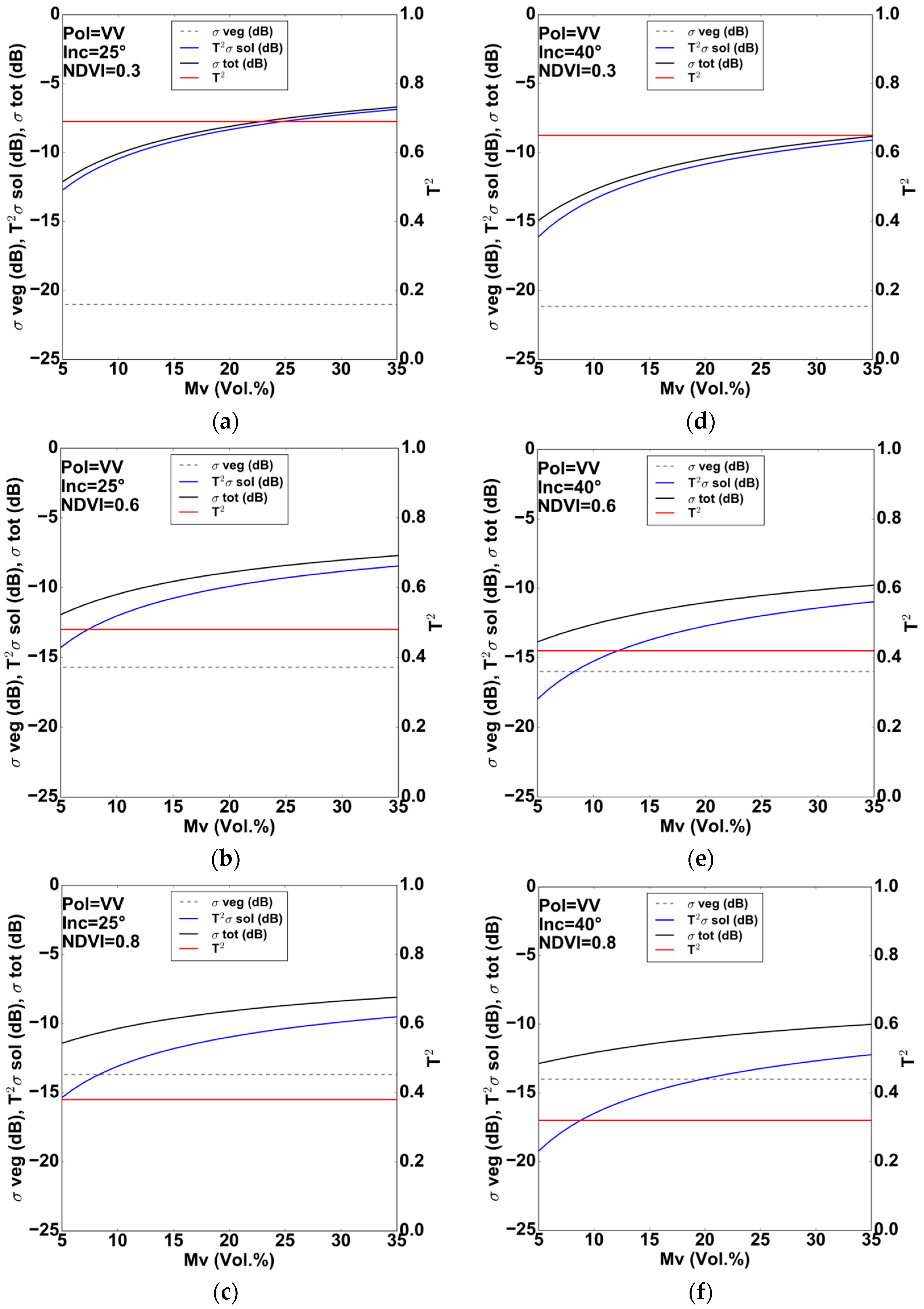
Figure 4.
Behavior of WCM components (σ0veg, T2σ0soil, and σ0tot) in VH polarization according to mv for 25° and 40° incidence angles. The soil roughness Hrms was fixed to 2 cm. (a): θ = 25° and NDVI = 0.3; (b): θ = 25° and NDVI = 0.6; (c): θ = 25° and NDVI = 0.8; (d): θ = 40° and NDVI = 0.3; (e): θ = 40° and NDVI = 0.6; (f): θ = 40° and NDVI = 0.8.
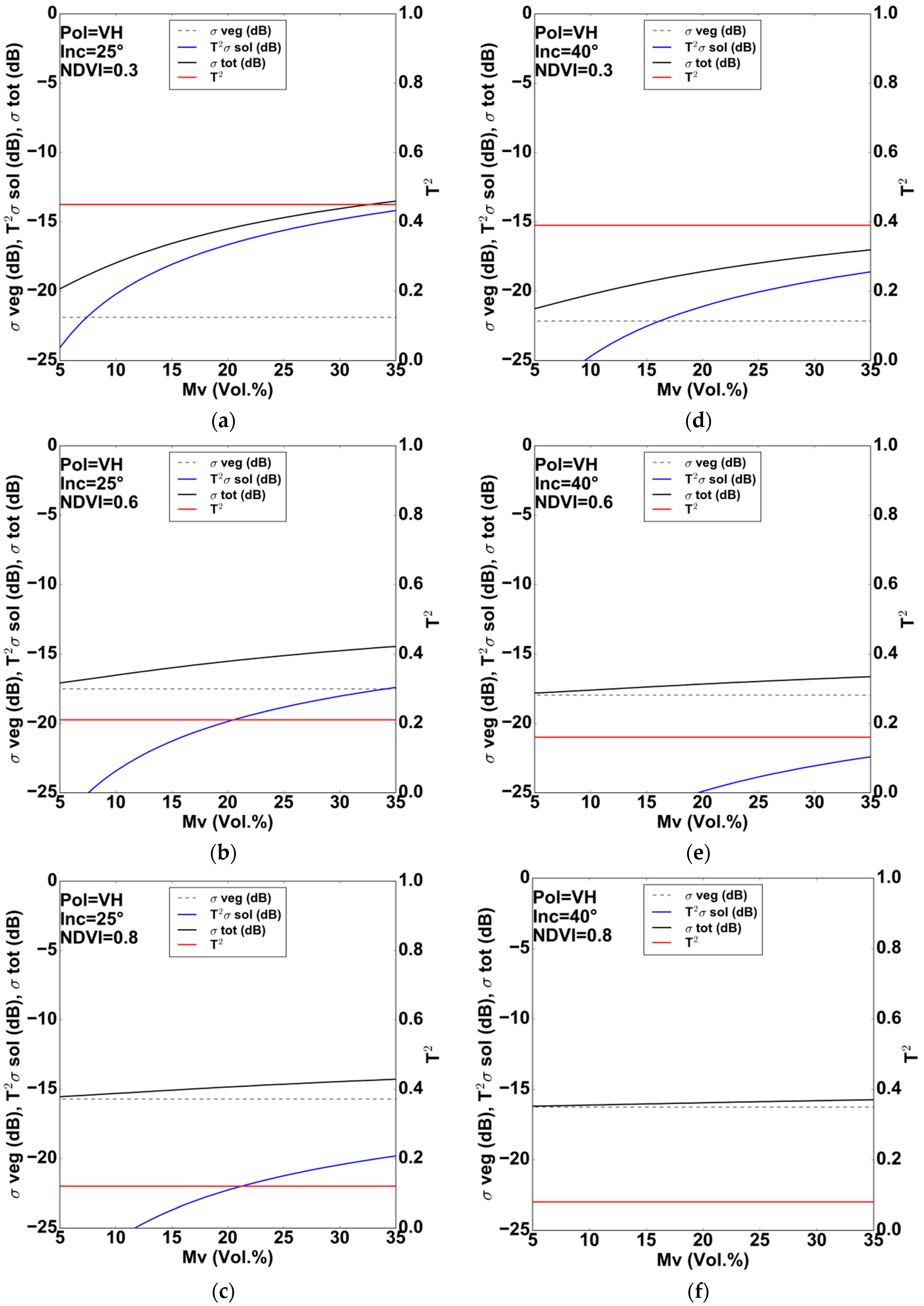
Figure 5.
Behavior of WCM components (σ0veg, T2σ0soil, and σ0tot) in VV and VH polarizations according to NDVI for 25° and 40° incidence angles, mv = 20 vol %, and Hrms = 2 cm. (a): VV and θ = 25°; (b): VV and θ = 40°; (c): VH and θ = 25°; (d): VH and θ = 40°.
Figure 5.
Behavior of WCM components (σ0veg, T2σ0soil, and σ0tot) in VV and VH polarizations according to NDVI for 25° and 40° incidence angles, mv = 20 vol %, and Hrms = 2 cm. (a): VV and θ = 25°; (b): VV and θ = 40°; (c): VH and θ = 25°; (d): VH and θ = 40°.


Table 1.
Description of the dataset used in this study.
| Site | SAR Sensor | Optical Sensor | Year | Number of Data |
|---|---|---|---|---|
| Tunisian site: Training dataset | ASAR | Landsat | 2009, 2010, 2011, 2012 | VV: 92 measurements |
| Tunisian site: Training dataset | Sentinel-1 | Landsat | 2015, 2016, 2017 | VV: 68 measurements VH: 68 measurements |
| French site: Validation dataset | Sentinel-1 | Sentinel-2 | 2016, 2017 | VV: 261 measurements VH: 261 measurements |
Table 2.
Fit of Water Cloud Model (WCM) parameters for each polarization (pq = VV and VH) using training dataset. N is the number of points used in the fitting.
Table 2.
Fit of Water Cloud Model (WCM) parameters for each polarization (pq = VV and VH) using training dataset. N is the number of points used in the fitting.
| V1 = V2 = NDVI | ||||||
|---|---|---|---|---|---|---|
| Polarization | Apq | Bpq | R2pq | RMSEpq (dB) | Biaspq (dB) | N |
| pq = VV | 0.0950 | 0.5513 | 0.55 | 1.55 | 0.18 | 160 |
| pq = VH | 0.0413 | 1.1662 | 0.63 | 1.30 | −0.17 | 68 |
Table 3.
Threshold values of NDVI at which vegetation contribution σ0veg dominates soil contribution T2σ0soil at VV and VH polarizations. Dash symbols mean that the σ0veg is always dominated by T2σ0soil (see Figure 3). The soil roughness Hrms was fixed to 2 cm.
Table 3.
Threshold values of NDVI at which vegetation contribution σ0veg dominates soil contribution T2σ0soil at VV and VH polarizations. Dash symbols mean that the σ0veg is always dominated by T2σ0soil (see Figure 3). The soil roughness Hrms was fixed to 2 cm.
| VV (25°) | VV (40°) | |||||||
| mv (vol %) | 5 | 10 | 20 | 30 | 5 | 10 | 20 | 30 |
| NDVI | 0.70 | - | - | - | 0.51 | 0.65 | - | - |
| VH (25°) | VH (40°) | |||||||
| mv (vol %) | 5 | 10 | 20 | 30 | 5 | 10 | 20 | 30 |
| NDVI | 0.27 | 0.39 | 0.51 | 0.60 | 0.19 | 0.27 | 0.36 | 0.41 |
© 2017 by the authors. Licensee MDPI, Basel, Switzerland. This article is an open access article distributed under the terms and conditions of the Creative Commons Attribution (CC BY) license (http://creativecommons.org/licenses/by/4.0/).
Share and Cite
MDPI and ACS Style
Baghdadi, N.; El Hajj, M.; Zribi, M.; Bousbih, S. Calibration of the Water Cloud Model at C-Band for Winter Crop Fields and Grasslands. Remote Sens. 2017, 9, 969. https://doi.org/10.3390/rs9090969
AMA Style
Baghdadi N, El Hajj M, Zribi M, Bousbih S. Calibration of the Water Cloud Model at C-Band for Winter Crop Fields and Grasslands. Remote Sensing. 2017; 9(9):969. https://doi.org/10.3390/rs9090969
Chicago/Turabian StyleBaghdadi, Nicolas, Mohammad El Hajj, Mehrez Zribi, and Safa Bousbih. 2017. "Calibration of the Water Cloud Model at C-Band for Winter Crop Fields and Grasslands" Remote Sensing 9, no. 9: 969. https://doi.org/10.3390/rs9090969
Note that from the first issue of 2016, this journal uses article numbers instead of page numbers. See further details here.