Impacts of Urbanization on Vegetation Phenology over the Past Three Decades in Shanghai, China


1
Department of Geography, University of North Carolina at Chapel Hill, Chapel Hill, NC 27599, USA
2
School of Ecological and Environmental Sciences, East China Normal University, Shanghai 200241, China
3
Shanghai Key Laboratory of Urbanization and Eco-Restoration, Shanghai 200241, China
*
Authors to whom correspondence should be addressed.
Remote Sens. 2017, 9(9), 970; https://doi.org/10.3390/rs9090970
Submission received: 23 July 2017
/
Revised: 11 September 2017
/
Accepted: 18 September 2017
/
Published: 20 September 2017
(This article belongs to the Special Issue Remote Sensing of Urban Ecology)
Abstract
:Vegetation phenology manifests the rhythm of annual plant life activities. It has been extensively studied in natural ecosystems. However, major knowledge gaps still exist in understanding the impacts of urbanization on vegetation phenology. This study addresses two questions to fill the knowledge gaps: (1) How does vegetation phenology vary spatially and temporally along a rural-to-urban transect in Shanghai, China, over the past three decades? (2) How do landscape composition and configuration affect those variations of vegetation phenology? To answer these questions, 30 m × 30 m mean vegetation phenology metrics, including the start of growing season (SOS), end of growing season (EOS), and length of growing season (LOS), were derived for urban vegetation using dense stacks of enhanced vegetation index (EVI) time series from images collected by Landsat 5–8 satellites from 1984 to 2015. Landscape pattern metrics were calculated using high spatial resolution aerial photos. We then used Pearson correlation analysis to quantify the associations between phenology patterns and landscape metrics. We found that vegetation in urban centers experienced advances of SOS for 5–10 days and delays of EOS for 5–11 days compared with those located in the surrounding rural areas. Additionally, we observed strong positive correlations between landscape composition (percentage of landscape area) of developed land and LOS of urban vegetation. We also found that the landscape configuration of local land cover types, especially patch density and edge density, was significantly correlated with the spatial patterns of vegetation phenology. These results demonstrate that vegetation phenology in the urban area is significantly different from its rural surroundings. These findings have implications for urban environmental management, ranging from biodiversity protection to public health risk reduction.
1. Introduction
Urbanization significantly alters Earth’s land surface condition and has profound impacts on regional-to-global terrestrial ecosystem processes and services [1,2,3]. Vegetation phenology, the interannual rhythm of the start, progress and ending of vegetation growth, manifests these impacts. Therefore, understanding the effect of urbanization on vegetation phenology is a critical step to study the broader influences of urbanization on the environment. Urban vegetation provides crucial ecosystem services, such as reducing noise, absorbing pollutants, serving as habitats for some migratory and local birds. Previous studies confirmed that urban areas experience higher temperature than the surrounding rural regions [4,5,6]. This phenomenon is known as the urban heat island (UHI) effect. An accurate knowledge of the impacts of UHI on vegetation phenology can help mitigate the vulnerability of urban ecosystem services. For example, quantifying the effects of UHI on vegetation phenology can reveal the potential phenological mismatches between vegetation, insects and birds at higher trophic levels [7,8], thus providing clues for biodiversity protection in the urban ecosystem. Moreover, vegetation phenology controls the timing of pollen production, and thus the allergy season in urban areas [9]. Understanding the urbanization-induced phenological changes can provide valuable information for public health risk forecasting [9,10].
Given the significant progress in detecting phenological changes of the natural ecosystems that are generally controlled by temperature [11,12,13] and precipitation [14,15], it remains less clear how the process of urbanization has altered vegetation phenology in the heterogeneous urban environment. Manipulative experiments and ground observations have documented earlier starts of growing seasons (SOS) and later ends of growing seasons (EOS) in the urban center than the surrounding rural areas [16,17]. While those studies provide important evidences of effects of urbanization on vegetation phenology, site-based observations cannot provide an assemble understanding of spatially-explicit phenological changes in urban areas due to the lack of standard data collection protocols and consistent data analysis methods [18]. Remote sensing observations offer consistent quantitative measurements of land surface properties, making long-term satellite observations ideal resources for monitoring vegetation phenology [19]. Many algorithms have been developed to estimate phenological metrics based on time series of vegetation indices derived from Advanced Very High Resolution Radiometer (AVHRR) and Moderate Resolution Imaging Spectroradiometer (MODIS) [20,21,22,23,24,25]. More specifically, studies have reported an increase of 7.6 days in the length of growing season (LOS) caused by urbanization in the Eastern United States [26]. Zhang et al. [27] found an increase of LOS by 15 days around urban centers, and the lengthening of LOS extends up to 10 km beyond urban margin. Zhou et al. [28] found SOS were 11.9 days earlier and EOS were 5.4 days later around urban centers than their surrounding rural areas in China’s 32 cities. However, our understanding of urban phenology with the coarse spatial resolution images in urban environments is limited due to the complexity of the urban environment. The localized heterogeneity in urban phenology changes as a result of spatial variations in urban land-cover/land-use (LCLU) composition and configuration cannot be revealed using coarse spatial resolution images.
The opening of the Landsat archive has enabled the pixel-wise long-term time series analyses at finer spatial resolution [29]. Fisher et al. [30] demonstrated that the average phenology of New England deciduous forests could be mapped at the Landsat scale using multitemporal Landsat observations that were organized by day of year (DOY). Melaas et al. [31,32] extended the algorithm in a way that allowed the detection of interannual variability in phenology and validated the method in North American temperate and boreal deciduous forest. These approaches have only recently been applied to urban areas [33,34], and there remain substantially unrealized potential for leveraging them to better understand how urbanization affects phenological changes. More importantly, landscape patterns not only reflect the urban development and their socioeconomic drivers [35,36,37], but also significantly influence UHI [38]. However, the relationship between landscape pattern and vegetation phenology is poorly understood. Therefore, this research aims to investigate the impacts of urbanization, as well as the urban landscape composition and configuration on vegetation phenology from 1984 to 2015 in Shanghai, China. We addressed the following two questions: (1) How does vegetation phenology vary spatially and temporally along a rural-to-urban transect over the past three decades? (2) How do landscape composition and configuration affect those variations of vegetation phenology? We hypothesize that not only the urban center has longer LOS, but also the landscape composition and configuration influence the spatial patterns of vegetation phenology.
2. Materials
2.1. Study Area
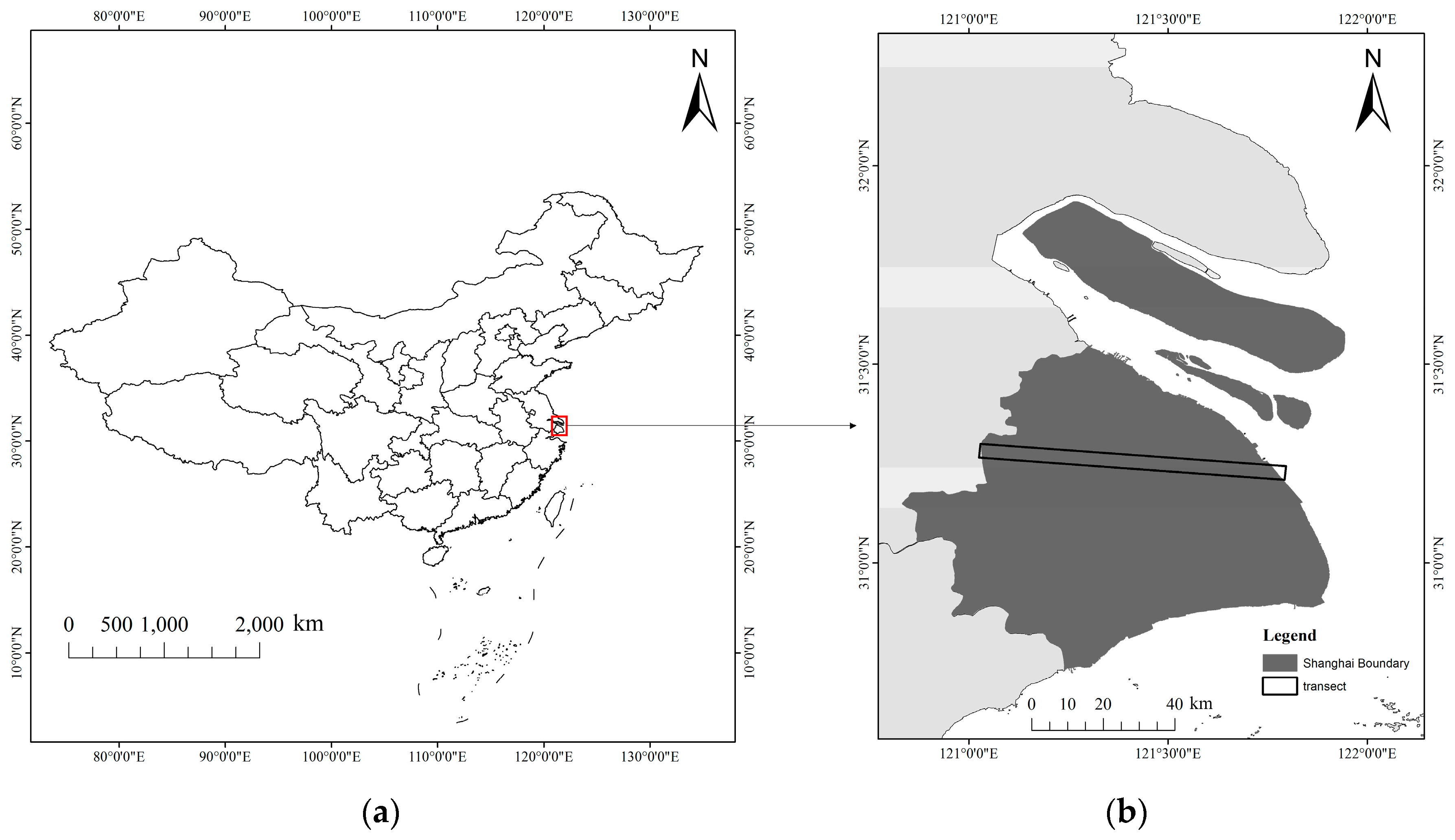
Our study area is located in Shanghai, China (Figure 1), covering 6340.5 km2. Shanghai is the most urbanized city in China. Elevation in the study region ranges from −27 to 63 m with an average of 4 m above sea level. According to the local climate record (1991–2010 data from the Central Weather Bureau of China), the climate in Shanghai is classified as subtropical monsoon climate with a mean annual temperature of 17.1 °C, and a mean annual precipitation of 1166.1 mm. The native vegetation in Shanghai is composed of subtropical evergreen broadleaf forest and evergreen broadleaf and deciduous broadleaf mixed forest [39]. We specifically focus on the impacts of landscape composition and configuration on spatio-temporal patterns of vegetation phenology along an east-west transect that runs through the urban center (Figure 1b). This transect represents the main axis of urban planning of Shanghai, covering the fastest urbanization regions, as well as the rural areas that belong to Shanghai administratively [37].
2.2. Data
We used all available images from two overlapping Landsat scenes (Path 118, Rows 38 and 39) covering Shanghai. The images come from Thematic Mapper (TM), Enhanced Thematic Mapper plus (ETM+), and the Operational Land Imager (OLI) sensors. All images were downloaded from the United States Geological Survey. We then converted the digital numbers to surface reflectance using the Landsat Ecosystem Disturbance Adaptive Processing System (LEDAPS) [40] and removed the pixels contaminated by clouds and their shadows using the Fmask algorithm [41]. After the preprocessing, the dataset included a total of 876 images spanning the period from 1984 to 2015. We also took advantage of the high spatial resolution (2.5 × 2.5 m) LCLU maps derived from aerial photos acquired in 1994, 2000 and 2005 along the transect (Figure 1b). The high spatial resolution LCLU maps can capture more accurately the landscape composition and configuration of the heterogeneous urban environment than those at the Landsat sensor spatial resolution [37]. The aerial photos were first classified into 48 LCLU classes in vector data formats based on visual interpretation [37]. The 48 LCLU classes were then converted into raster grids and aggregated into 8 broader classes, including agriculture (AG), industry (IN), residential (RE), public facility (PF), water (WA), vegetation (VG), traffic (TR), and the others (OT) [37]. The overall accuracies for 1994, 2000, and 2005 LCLU maps are 95.8%, 95.3%, and 93.9%, respectively [37]. Table 1 shows the percentage of land cover types in these maps. In addition, we utilized the 90-m spatial resolution digital elevation model (DEM) data downloaded from the Shuttle Radar Topography Mission (SRTM) to improve the LCLU classification of the transect with Landsat imagery.
3. Methods
3.1. Landsat Image Classification with AASG
In order to understand the effect of urbanization on vegetation phenology with Landsat images, we need to separate the land surface into different LCLU types. We used the automatic adaptive signature generalization (AASG) [42,43] algorithm to classify the multi-season Landsat images into five land cover types, including water, urban vegetation, cropland, developed land, and barren land. Surface reflectance images from bands 1–5, and 7 of TM and ETM+ sensors, bands 2–7 of OLI sensor were used. In order to use AASG to classify the entire time series of images, we need to first generate a reference map for the algorithm [42,43]. We selected training samples from Landsat images acquired in year 1995, and classified the stacked multi-season images using a random forest (RF) classifier [44]. We then utilized the 1995 LCLU map as the reference for classification with AASG for 2000, 2005, 2010, and 2015 using the multi-season Landsat surface reflectance images as inputs for the respective years. Each set of multi-season Landsat images consisted of images from early-, mid-, and late-growing season (Table 2). Mid-season cloud-free images for years 2005 and 2010, and early-season and late-season cloud free images for year 2015 were not available, so we selected images from years 2006, 2011, and 2014 as proxies, respectively. The gaps in ETM+ SLC-off images were recovered using multi-temporal regression analysis [45]. In addition, we included the topographic wetness index (TWI) derived from DEM as a data layer and stacked it with the multi-season composite image. The classified LCLU maps were then utilized to provide masks to separate urban vegetation from other land cover types for phenology analysis.
3.2. Mean Phenology Models for Urban Vegetation
Due to the fact that Landsat satellites do not provide images frequent enough for phenological analysis on a year-by-year basis, we divided our time frame into five time periods, including 1984–1995, 1996–2000, 2001–2005, 2006–2010, and 2011–2015. We stacked all the available Landsat EVI images within each time period by DOY. We derived the mean phenology for urban vegetation by fitting the sigmoid-family curves to the stacks of Landsat images for each time period [30]. The uneven lengths of the time periods resulted from the number of images available so that there are sufficient data points to obtain the mean vegetation phenology in each time period. The images we used to fit the phenological curves were EVI-derived from Landsat surface reflectance. We used EVI because it provides a larger range of variations in densely vegetated area compared with other spectral vegetation indices [46].
For urban vegetation, a difference logistic function with six parameters was used to characterize the mean phenology at each pixel [21,22,24,30,47]:
where is the DOY, is the background EVI value, is the amplitude of the smoothed EVI time series, and are the fitting parameters for the spring onset period, and and control the fall senescence period.
Equation (1) was fitted at each urban vegetation pixel using an iteratively-weighted, nonlinear least squares regression [21,48]. SOS and EOS of urban vegetation are defined as the dates when reached the inflection points of the fitted curve in the spring rising and autumn falling periods of EVI time series [21,30]. LOS is defined as the difference of EOS and SOS. It is important to note that the SOS, EOS, and LOS used in this study were satellite-based proxies of seasonal development stages of urban vegetation in the real world. These phenological metrics can be very different from other indicators, such as the date of bud break. As long as these metrics are identified in a consistent manner, the subsequent analyses should be robust.
3.3. Landscape Pattern Metrics
Numerous landscape pattern metrics have been developed to characterize the composition and configuration of land cover types in the urban environment [49,50,51,52]. We selected the most commonly used landscape composition metrics, the percentage of landscape area (PLAND) and two other diversity metrics: Shannon’s diversity index (SHDI) and Shannon’s evenness index (SHEI) [51]. Landscape configuration metrics [51] used in this study included edge density (ED), patch density (PD), landscape shaped index (LSI), contagion (CONTAG)m and clumpiness (CLUMPY). They are given in Table 3. Detailed descriptions and calculations of composition and configuration metrics can be found in McGarigal et al. [51]. These metrics were selected because they were proven to be significantly related with urban microclimatological factors [38,53].
We used the LCLU map derived from the aerial photos along the transect (Figure 1b) to calculate the landscape pattern metrics. The transect was divided into 26 blocks, each of which measures 5 × 5 km in size with 2.5 km overlaps with neighboring blocks. These blocks were delineated to capture the spatial patterns of landscape metrics along the rural-to-urban gradient [37]. The landscape composition and configuration metrics in each block were calculated using FRAGSTATS [51] for years 1995, 2000, and 2005. Class level metrics for each of the eight LCLU types and landscape level metrics were included in the calculation.
3.4. Analyses
To explore the impacts of urbanization on spatial patterns of vegetation phenology, we calculated the mean value of Landsat level phenology metrics (SOS, EOS, and LOS) in each 5 × 5 km block. We quantified how SOS, EOS, and LOS within each block varied as a function of distance from urban center along the transect. To examine the temporal patterns of vegetation phenology over the past three decades, we calculated the standardized anomalies (Equation (2)) from mean LOS across the five time periods:
where subscript is the index for different time intervals. are the LOS metrics for the five time periods, including 1984–1995, 1996–2000, 2001–2005, 2006–2010, and 2011–2015, respectively. Standardized anomalies between −1 and 1 represented no change of LOS, and standardized anomalies greater than 1 were marked as increases of LOS, while standardized anomalies less than −1 were identified as decreases of LOS. Pearson correlation coefficients were also calculated to examine the associations between mean phenology metrics and composition and configuration of local LCLU at both class and landscape levels for the years 1995, 2000, and 2005, respectively.
4. Results
4.1. AASG Classification Results
Figure 2 presents the results of AASG classification in the east-west transect for years 1995, 2000, 2005, 2010, and 2015, respectively. The overall accuracy for the land cover maps ranged from 74% to 84%, more details about confusion matrix can be found in the supplementary material (Tables S1–S5). The east-west transect had experienced a dramatic urban expansion from 1995 to 2015. Table 4 shows the percentages of land cover types in these maps. A large proportion of the cropland have been replaced by developed land.
4.2. Phenological Curves
Figure 3 presents the mean phenology model of the five time periods based on multi-temporal Landsat images for a pixel of typical urban vegetation. Phenology curves in Figure 3 clearly shows inflection points (also mid-points between maximum and minimum of the fitted EVI time series for the difference logistic function) in the spring greening-up and fall senescence. These inflection points can be easily and consistently identified from the phenology curves and are considered as the SOS and EOS dates in this study. Figure 3 also shows that the rate of change in EVI along the growing season varies from period to period.
4.3. Spatio-Temporal Patterns of Vegetation Phenology
Figure 4, Figure 5 and Figure 6 present images showing the SOS, EOS, and LOS at Landsat spatial resolution for urban vegetation along the east-west transect over the five periods (the gray areas are non-vegetation land or missing data). Figure 4, Figure 5 and Figure 6 clearly show that the phenology cycle in the urban centers starts earlier, and ends later, leading to a longer growing season when compared with the surrounding less-developed regions.
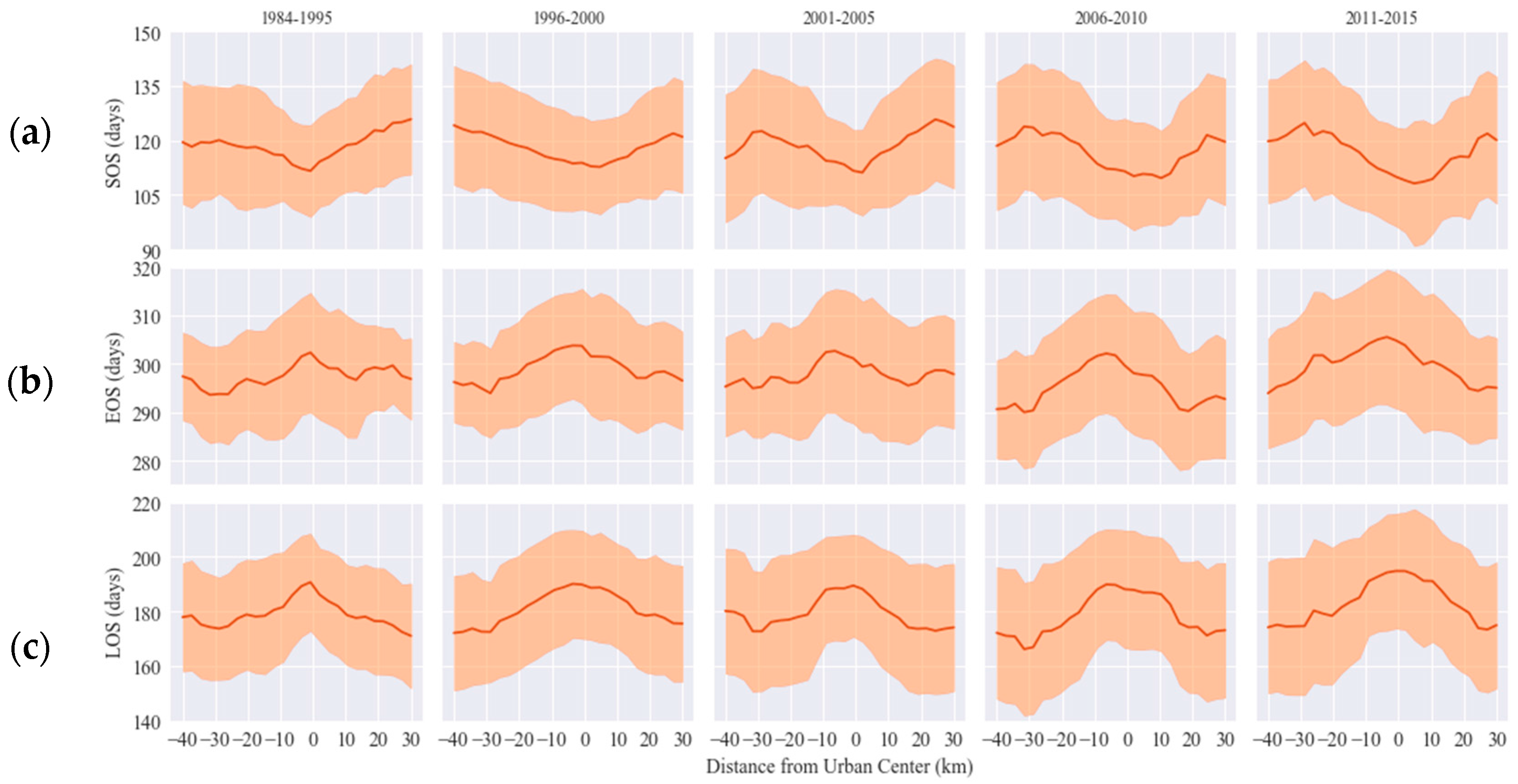
Figure 7 shows the mean and standard deviation of the phenological metrics along the transect. We see a clear pattern that vegetation in the urban center greens up earlier and senesces later compared to vegetation located in the rural areas for all five time periods. On average, SOS occurs 5–10 days earlier, and EOS appears about 5–11 days later, leading to LOS being longer by about 10–21 days in the urban center compared with the rural regions. In addition, we see substantial localized variations in SOS, EOS, and LOS along the transect, probably caused by the spatial heterogeneity of the urban environment. The local variations in phenology metrics can be as much as 10 days.
Table 5 shows the percentages of longer LOS (standardized anomalies greater than 1), shorter LOS (standardized anomalies smaller than −1), and no-change of LOS (standardized anomalies between −1 and 1) within the transect for urban vegetation in the five periods. The percentage of longer LOS seems to increase while the percentage of shorter LOS seems to decrease through the five periods.
4.4. Pearson Correlations between SOS, EOS, LOS, and Landscape Metrics
Table 6 shows Pearson correlation coefficients between landscape level metrics and phenology metrics for urban vegetation in the three time periods including 1984–1995, 1996–2000, and 2001–2005 when we have high spatial resolution air photos. According to Table 6, CONTAG is significantly correlated with phenology metrics, except for the 2001–2005 interval. The correlations between SHEI, SHDI, and phenology metrics are also significant during the 1984–1994 and 1996–2000 intervals (except SOS during 1984–1995). PD is significantly correlated with phenology metrics, except during the 1984–1995 interval. More specifically, both PD and CONTAG have positive correlations with SOS, while having negative correlations with EOS and, as a result, negative correlations with LOS. Both SHDI and SHEI exhibit the opposite correlations with phenology metrics compared with CONTAG and PD. The correlations for both LSI and ED with phenology metrics are more complicated as they are not consistent across three time periods. For example, LSI is negatively correlated with SOS during 1984–1995, but it is positively correlated with SOS during 2001–2005.
Table 7 shows the Pearson correlation coefficients between class-level pattern metrics and phenology metrics for urban vegetation in three time periods, including 1984–1995, 1996–2000, and 2001–2005. The class-level PLAND of RE and PF are significantly negatively related with SOS and positively related with EOS, and, thus, positively with LOS. Those correlations are also consistent across three time periods. Meanwhile, higher PLAND of both IN and TR are significantly associated with earlier SOS and later EOS and, as a result, longer LOS except during 2001–2005. In contrast, PLAND of both AG and WA show the opposite correlations with phenology metrics. The higher PLAND of AG/WA tends to be correlated with shorter growing seasons (LOS) from both later greening (SOS) and earlier senescence (EOS). As for the PLAND for VG, the correlations are only significant during 1984–1995.
PD for PF exhibits a significant negative correlation with SOS and a positive correlation with EOS, thus, a positive correlation with LOS. The correlations are consistent across three time intervals. In comparison, the signs of correlations between PD for AG/VG and phenology metrics are opposite to the signs of correlations between PD for PF. As for PD of other LCLU types, the correlations between PD and phenology metrics are not consistent. For example, PD for IN in 1984–1995 is negatively correlated with SOS, while it is positively correlated with SOS in 2001–2005.
ED for RE, PF, IN, and TR are negatively correlated with SOS, but they are positively correlated with EOS, thus, positively correlated with LOS. These LCLU types are mostly dominated by impervious surfaces, contributing to UHI effects. In addition, vegetation associated with these land-use types are often actively managed, particularly irrigation and fertilization. Therefore, it is not surprising that higher ED for these land-use types lead to longer LOS. Meanwhile, higher ED for WA, VG and AG tend to have later SOS, earlier EOS and, thus, shorter LOS. LSI for PF, IN, TR, VG, and WA have similar correlations with phenology metrics as ED does. However, LSI for RE only has significant correlations with phenological metrics in 1996–2000.
CLUMPY for LCLU types does not show consistent significant correlation across three time intervals except for WA and VG. Specifically, correlations between phenology metrics and CLUMPY for WA/VG indicate that higher CLUMPY values have earlier SOS, later EOS and, thus, longer LOS.
5. Discussion
This research derived the mean phenological metrics (SOS, EOS, and LOS) for urban vegetation along a rural-to-urban transect in Shanghai from Landsat images by fitting sigmoid-family functions on EVI time series organized by DOY from multiple years. While this approach did not allow for detection of inter-annual variations within each time period, it produced 30 m × 30 m phenology metrics within each time intervals. Figure 3 shows that these functions capture the temporal patterns of EVI very well, and provide a means to consistently identify the phenological metrics across the time intervals. We also clearly see that rates of change in EVI were different across different time periods, which indicates that the assumptions (maximums and shapes of smoothed EVI curve remain the same from year to year) in Landsat phenology algorithm developed by Melaas et al. [31] may not hold in the heterogeneous urban environments. However, the greatest weakness of this study is the lack of data for accuracy assessment. This is a common problem for large area phenology study based on satellite images. However, the general spatiotemporal patterns we identified along the rural to urban gradient fit our expectation, although we do not know the specific picture for Shanghai without this study.
Recent research has suggested that the growing season of vegetation in cities is longer compared with the surrounding rural regions because of UHI effects [9,17,26,27,33,34]. Our results support this conclusion, providing a refined characterization of interactions between composition and configuration of local LCLU types and spatial patterns of vegetation phenology. Our hypothesis suggested that landscape metrics influenced vegetation phenology was supported by the significant correlations between phenology metrics and landscape metrics at both landscape level and class level. Therefore, UHI is not the only factor that influences phenology of urban vegetation. Specifically, we found that an increase in PD at the landscape level had a shorter growing season. This can be explained by the negative correlation between the heterogeneity and the land surface temperature (LST) [38]. Since vegetation phenology is very sensitive to temperature [33,54], higher LST leads to earlier SOS and later EOS, thus, a longer LOS. However, an increase of heterogeneity can reduce the LST [38], thus weakening the UHI effect on the growing season. However, we also found low CONTAG and high SHEI/SHDI, which indicated high heterogeneity, had a longer growing season. This may be caused by land conversions from agricultural land to developed land such as RE, PF, TR, and IN. Those land conversions increased the varieties of patch types in the transect, thus affecting CONTAG and SHEI/SHDI, but they might not influence PD. The land conversions also enhanced the effects of UHI on vegetation phenology, thus ending up with a longer growing season. In addition, we found inconsistencies in the correlation between both LSI and ED with SOS in different time intervals at the landscape scale. This may be due to the rapid and complicated urbanization process in Shanghai. As described in Li et al. [37], urban regions in Shanghai were characterized with a complex-shaped (high LSI/ED) landscape at first and then associated with a simpler (low LSI/ED) one later on. Since areas around the urban center always experienced longer LOS compared with rural regions, the correlations between LSI/ED and LOS in 1984–1995 were the opposite to those in 2001–2005.
At the class level, our results suggested land cover composition significantly affected the vegetation phenology. The increase in the percentage of residential land, public facilities, industrial land, and traffic land in a given landscape significantly advanced SOS and delayed EOS, therefore, resulting in longer LOS as these land cover types tended to have higher LST [38,55,56,57]. The increase of proportion of water and agricultural land, on the other hand, had later SOS and earlier EOS since those lands had lower LST [38,55,56,57]. More importantly, our results found that vegetation phenology was not only influenced by local land cover composition, but was also influenced by their spatial configuration. Spatial configuration can affect the flow of energy and energy exchange among different land cover types [53,58], therefore, altering vegetation phenology. For example, the increase of PD, ED, and LSI of public facility and industrial land leads to an increase of LOS because the increase of edges and patches can lead to the developed land absorbing solar energy more efficiently [59], thus increasing the LST and lengthening LOS. Meanwhile, the PD and ED of urban vegetation were negatively correlated with LOS because the increase of vegetation edges and patches enhanced energy exchanges and reduced LST, thus resulting in a shorter growing season. Those findings indicate that habitats could be created in urban environment to minimize the effect of UHI on plant phenology so that the phenological mismatch between different trophic levels could be mitigated for migratory bird nesting [7,8]. Additionally, we observed inconsistencies of correlations between different phenology metrics and class level landscape metrics. Those inconsistencies could be due to different sensitivities between spring onset and fall senescence to LST [28,30].
In addition to the lack of data for validation, this study also has some other limitations. First, we did not take vegetation species composition into account when describing the phenology pattern and its interaction with landscape metrics. Exotic, ornamental, and invasive vegetation species are common in urban landscapes [60]. The composition of vegetation species with different phenological characteristics can introduce bias in the spatial analysis of phenology patterns. Second, this research cannot disaggregate the effects of climate change from UHI effects as global warming could enhance UHI effects. For example, the temporal changes in Table 5 were the results of combined effects of climate change and UHI.
6. Conclusions
We derived the mean phenology (SOS, EOS, and LOS) of urban vegetation at 30-m spatial resolution based on multi-year Landsat images along an east-west transect that runs through the center of Shanghai, China during 1984–2015. Landscape composition and configuration metrics along the transect were derived from high spatial resolution aerial photos. We found that (1) average SOS of urban vegetation occurred 5–10 days earlier and EOS appeared 5–11 days later, causing LOS longer about 10–21 days in urban center compared with those of the rural counterparts. (2) Based on the statistics of the standardized anomalies across five time periods, 12.6% of the urban vegetation in the transect experienced longer growing seasons in the time interval of 1984–1995, while 22.2% experienced longer growing seasons in the time interval of 2011–2015. (3) Urban landscape structure influences the phenology of urban vegetation. At the landscape level, the increase of patch density was associated with later SOS and earlier EOS for urban vegetation, thus, a shorter LOS. At the class scale, increasing the percentage of developed land correlates with advanced spring onset and delayed fall senescence, thus, a longer season, while higher proportions of agricultural land and water led to later SOS, earlier EOS and, thus, shorter LOS. Meanwhile, higher edge density and patch density of developed land had positive effects on LOS, while those of urban vegetation had negative effects on LOS. Those findings revealed that the composition and configuration of urban LCLU significantly influenced the spatial pattern of vegetation phenology.
Supplementary Materials
The following are available online at www.mdpi.com/2072-4292/9/9/970/s1.
Acknowledgments
This research was partly supported by the US National Science Foundation (Grant No. DEB-1313756) and the Natural Science Foundation of China (Grant No. 31528004 to Conghe Song and Grant No. 31370482 to Junxiang Li).
Author Contributions
Conghe Song and Junxiang Li conceived and designed the experiments; Tong Qiu performed the experiments and analyzed the data; Tong Qiu wrote the paper; Junxiang Li contributed materials; and Conghe Song and Junxiang Li improved the manuscript.
Conflicts of Interest
The authors declare no conflict of interest.
Abbreviations
The following abbreviations are used in this manuscript:
| AG | Agriculture |
| AASG | Automatic Adaptive Signature Generalization |
| AVHRR | Advanced Very High Resolution Radiometer |
| CLUMPY | Clumpyness |
| CONTAG | Contagion |
| DEM | Digital Elevation Model |
| DOY | Day of Year |
| ED | Edge Density |
| EOS | End of Season |
| ETM+ | Enhanced Thematic Mapper Plus |
| EVI | Enhanced Vegetation Index |
| IN | Industry Area |
| LCLU | Land-cover/land-use |
| LOS | Length of Season |
| LSI | Landscape Shape Index |
| MODIS | Moderate Resolution Imaging Spectroradiometer |
| OLI | Operational Land Imager |
| OT | Others |
| PD | Patch Density |
| PF | Public Facility |
| PLAND | Percentage of Landscape area |
| RE | Residential Area |
| RF | Random Forest |
| SHDI | Shannon’s Diversity Index |
| SHEI | Shannon’s Evenness Index |
| SOS | Start of Season |
| SRTM | Shuttle Radar Topography Mission |
| TM | Thematic Mapper |
| TR | Traffic Area |
| TWI | Topographic Wetness Index |
| VG | Vegetation |
| WA | Water |
References
- Foley, J.A.; DeFries, R.; Asner, G.P.; Barford, C.; Bonan, G.; Carpenter, S.R.; Chapin, F.S.; Coe, M.T.; Daily, G.C.; Gibbs, H.K.; et al. Global consequences of land use. Science 2005, 309, 570–574. [Google Scholar] [CrossRef] [PubMed]
- Grimm, N.B.; Faeth, S.H.; Golubiewski, N.E.; Redman, C.L.; Wu, J.G.; Bai, X.M.; Briggs, J.M. Global change and the ecology of cities. Science 2008, 319, 756–760. [Google Scholar] [CrossRef] [PubMed]
- Seto, K.C.; Guneralp, B.; Hutyra, L.R. Global forecasts of urban expansion to 2030 and direct impacts on biodiversity and carbon pools. Proc. Natl. Acad. Sci. USA 2012, 109, 16083–16088. [Google Scholar] [CrossRef] [PubMed]
- Arnfield, A.J. Two decades of urban climate research: A review of turbulence, exchanges of energy and water, and the urban heat island. Int. J. Climatol. 2003, 23, 1–26. [Google Scholar] [CrossRef]
- Oke, T.R. City size and the urban heat island. Atmos. Environ. 1973, 7, 769–779. [Google Scholar] [CrossRef]
- Oke, T.R. The energetic basis of the urban heat island. Q. J. R. Meteorol. Soc. 1982, 108, 1–24. [Google Scholar] [CrossRef]
- Miller-Rushing, A.J.; Hoye, T.T.; Inouye, D.W.; Post, E. The effects of phenological mismatches on demography. Philos. Trans. R. Soc. B Biol. Sci. 2010, 365, 3177–3186. [Google Scholar] [CrossRef] [PubMed]
- Thackeray, S.J.; Henrys, P.A.; Hemming, D.; Bell, J.R.; Botham, M.S.; Burthe, S.; Helaouet, P.; Johns, D.G.; Jones, I.D.; Leech, D.I.; et al. Phenological sensitivity to climate across taxa and trophic levels. Nature 2016, 535, 241–245. [Google Scholar] [CrossRef] [PubMed]
- Neil, K.; Wu, J. Effects of urbanization on plant flowering phenology: A review. Urban Ecosyst. 2006, 9, 243–257. [Google Scholar] [CrossRef]
- Cecchi, L.; D’Amato, G.; Maesano, I.A. Climate, Urban Air Pollution, and Respiratory Allergy. In Climate Vulnerability: Understanding and Addressing Threats to Essential Resources; Elsevier: Amsterdam, The Netherlands, 2013; Volume 1, pp. 105–113. [Google Scholar]
- Schwartz, M.D.; Ahas, R.; Aasa, A. Onset of spring starting earlier across the Northern Hemisphere. Glob. Chang. Biol. 2006, 12, 343–351. [Google Scholar] [CrossRef]
- Zhang, X.Y.; Friedl, M.A.; Schaaf, C.B.; Strahler, A.H. Climate controls on vegetation phenological patterns in northern mid- and high latitudes inferred from MODIS data. Glob. Chang. Biol. 2004, 10, 1133–1145. [Google Scholar] [CrossRef]
- Zhang, X.Y.; Tarpley, D.; Sullivan, J.T. Diverse responses of vegetation phenology to a warming climate. Geophys. Res. Lett. 2007, 34. [Google Scholar] [CrossRef]
- Guan, K.; Wood, E.F.; Medvigy, D.; Kimball, J.; Pan, M.; Caylor, K.K.; Sheffield, J.; Xu, X.; Jones, M.O. Terrestrial hydrological controls on land surface phenology of African savannas and woodlands. J. Geophys. Res. Biogeosci. 2014, 119, 1652–1669. [Google Scholar] [CrossRef]
- Zhang, X.Y.; Friedl, M.A.; Schaaf, C.B.; Strahler, A.H.; Liu, Z. Monitoring the response of vegetation phenology to precipitation in Africa by coupling MODIS and TRMM instruments. J. Geophys. Res. Atmos. 2005, 110. [Google Scholar] [CrossRef]
- Jochner, S.C.; Sparks, T.H.; Estrella, N.; Menzel, A. The influence of altitude and urbanisation on trends and mean dates in phenology (1980–2009). Int. J. Biometeorol. 2012, 56, 387–394. [Google Scholar] [CrossRef] [PubMed]
- Mimet, A.; Pellissier, V.; Quenol, H.; Aguejdad, R.; Dubreuil, V.; Roze, F. Urbanisation induces early flowering: Evidence from Platanus acerifolia and Prunus cerasus. Int. J. Biometeorol. 2009, 53, 287–298. [Google Scholar] [CrossRef] [PubMed]
- Gill, A.L.; Gallinat, A.S.; Sanders-DeMott, R.; Rigden, A.J.; Short Gianotti, D.J.; Mantooth, J.A.; Templer, P.H. Changes in autumn senescence in Northern Hemisphere deciduous trees: A meta-analysis of autumn phenology studies. Ann. Bot. 2015, 116, 875–888. [Google Scholar] [CrossRef] [PubMed]
- De Beurs, K.M.; Henebry, G.M. Land surface phenology, climatic variation, and institutional change: Analyzing agricultural land cover change in Kazakhstan. Remote Sens. Environ. 2004, 89, 497–509. [Google Scholar] [CrossRef]
- Cong, N.; Piao, S.; Chen, A.; Wang, X.; Lin, X.; Chen, S.; Han, S.; Zhou, G.; Zhang, X. Spring vegetation green-up date in China inferred from SPOT NDVI data: A multiple model analysis. Agric. For. Meteorol. 2012, 165, 104–113. [Google Scholar] [CrossRef]
- Dannenberg, M.P.; Song, C.; Hwang, T.; Wise, E.K. Empirical evidence of El Nino-Southern Oscillation influence on land surface phenology and productivity in the western United States. Remote Sens. Environ. 2015, 159, 167–180. [Google Scholar] [CrossRef]
- Hwang, T.; Song, C.; Vose, J.M.; Band, L.E. Topography-mediated controls on local vegetation phenology estimated from MODIS vegetation index. Landsc. Ecol. 2011, 26, 541–556. [Google Scholar] [CrossRef]
- Jönsson, P.; Eklundh, L. TIMESAT—A program for analyzing time-series of satellite sensor data. Comput. Geosci. 2004, 30, 833–845. [Google Scholar] [CrossRef]
- Zhang, X.Y.; Friedl, M.A.; Schaaf, C.B.; Strahler, A.H.; Hodges, J.C.F.; Gao, F.; Reed, B.C.; Huete, A. Monitoring vegetation phenology using MODIS. Remote Sens. Environ. 2003, 84, 471–475. [Google Scholar] [CrossRef]
- White, M.A.; de Beurs, K.M.; Didan, K.; Inouye, D.W.; Richardson, A.D.; Jensen, O.P.; O’Keefe, J.; Zhang, G.; Nemani, R.R.; van Leeuwen, W.J.D.; et al. Intercomparison, interpretation, and assessment of spring phenology in North America estimated from remote sensing for 1982–2006. Glob. Chang. Biol. 2009, 15, 2335–2359. [Google Scholar] [CrossRef]
- White, M.A.; Nemani, R.R.; Thornton, P.E.; Running, S.W. Satellite evidence of phenological differences between urbanized and rural areas of the eastern United States deciduous broadleaf forest. Ecosystems 2002, 5, 260–273. [Google Scholar] [CrossRef]
- Zhang, X.Y.; Friedl, M.A.; Schaaf, C.B.; Strahler, A.H.; Schneider, A. The footprint of urban climates on vegetation phenology. Geophys. Res. Lett. 2004, 31. [Google Scholar] [CrossRef]
- Zhou, D.; Zhao, S.; Zhang, L.; Liu, S. Remotely sensed assessment of urbanization effects on vegetation phenology in China’s 32 major cities. Remote Sens. Environ. 2016, 176, 272–281. [Google Scholar] [CrossRef]
- Woodcock, C.E.; Allen, R.; Anderson, M.; Belward, A.; Bindschadler, R.; Cohen, W.; Gao, F.; Goward, S.N.; Helder, D.; Helmer, E.; et al. Free access to Landsat imagery. Science 2008, 320, 1011. [Google Scholar] [CrossRef] [PubMed]
- Fisher, J.I.; Mustard, J.F.; Vadeboncoeur, M.A. Green leaf phenology at Landsat resolution: Scaling from the field to the satellite. Remote Sens. Environ. 2006, 100, 265–279. [Google Scholar] [CrossRef]
- Melaas, E.K.; Friedl, M.A.; Zhu, Z. Detecting interannual variation in deciduous broadleaf forest phenology using Landsat TM/ETM plus data. Remote Sens. Environ. 2013, 132, 176–185. [Google Scholar] [CrossRef]
- Melaas, E.K.; Sulla-Menashe, D.; Gray, J.M.; Black, T.A.; Morin, T.H.; Richardson, A.D.; Friedl, M.A. Multisite analysis of land surface phenology in North American temperate and boreal deciduous forests from Landsat. Remote Sens. Environ. 2016, 186, 452–464. [Google Scholar] [CrossRef]
- Melaas, E.K.; Wang, J.A.; Miller, D.L.; Friedl, M.A. Interactions between urban vegetation and surface urban heat islands: A case study in the Boston metropolitan region. Environ. Res. Lett. 2016, 11. [Google Scholar] [CrossRef]
- Zipper, S.C.; Schatz, J.; Singh, A.; Kucharik, C.J.; Townsend, P.A.; Loheide, S.P., II. Urban heat island impacts on plant phenology: Intra-urban variability and response to land cover. Environ. Res. Lett. 2016, 11. [Google Scholar] [CrossRef]
- Jenerette, G.D.; Wu, J. Analysis and simulation of land-use change in the central Arizona—Phoenix region, USA. Landsc. Ecol. 2001, 16, 611–626. [Google Scholar] [CrossRef]
- Seto, K.C.; Fragkias, M. Quantifying spatiotemporal patterns of urban land-use change in four cities of China with time series landscape metrics. Landsc. Ecol. 2005, 20, 871–888. [Google Scholar] [CrossRef]
- Li, J.; Li, C.; Zhu, F.; Song, C.; Wu, J. Spatiotemporal pattern of urbanization in Shanghai, China between 1989 and 2005. Landsc. Ecol. 2013, 28, 1545–1565. [Google Scholar] [CrossRef]
- Li, J.X.; Song, C.H.; Cao, L.; Zhu, F.G.; Meng, X.L.; Wu, J.G. Impacts of landscape structure on surface urban heat islands: A case study of Shanghai, China. Remote Sens. Environ. 2011, 115, 3249–3263. [Google Scholar] [CrossRef]
- Gao, J. Study on the basic characteristics of natural vegetation, vegetation regionalization and protection of Shanghai. Geogr. Res. 1997, 16, 82–88. [Google Scholar]
- Masek, J.G.; Huang, C.; Wolfe, R.; Cohen, W.; Hall, F.; Kutler, J.; Nelson, P. North American forest disturbance mapped from a decadal Landsat record. Remote Sens. Environ. 2008, 112, 2914–2926. [Google Scholar] [CrossRef]
- Zhu, Z.; Woodcock, C.E. Object-based cloud and cloud shadow detection in Landsat imagery. Remote Sens. Environ. 2012, 118, 83–94. [Google Scholar] [CrossRef]
- Dannenberg, M.; Hakkenberg, C.; Song, C. Consistent Classification of Landsat Time Series with an Improved Automatic Adaptive Signature Generalization Algorithm. Remote Sens. 2016, 8, 691. [Google Scholar] [CrossRef]
- Gray, J.; Song, C. Consistent classification of image time series with automatic adaptive signature generalization. Remote Sens. Environ. 2013, 134, 333–341. [Google Scholar] [CrossRef]
- Rodriguez-Galiano, V.F.; Chica-Olmo, M.; Abarca-Hernandez, F.; Atkinson, P.M.; Jeganathan, C. Random Forest classification of Mediterranean land cover using multi-seasonal imagery and multi-seasonal texture. Remote Sens. Environ. 2012, 121, 93–107. [Google Scholar] [CrossRef]
- Zeng, C.; Shen, H.; Zhang, L. Recovering missing pixels for Landsat ETM+ SLC-off imagery using multi-temporal regression analysis and a regularization method. Remote Sens. Environ. 2013, 131, 182–194. [Google Scholar] [CrossRef]
- Huete, A.; Didan, K.; Miura, T.; Rodriguez, E.P.; Gao, X.; Ferreira, L.G. Overview of the radiometric and biophysical performance of the MODIS vegetation indices. Remote Sens. Environ. 2002, 83, 195–213. [Google Scholar] [CrossRef]
- Nijland, W.; Bolton, D.K.; Coops, N.C.; Stenhouse, G. Imaging phenology; scaling from camera plots to landscapes. Remote Sens. Environ. 2016, 177, 13–20. [Google Scholar] [CrossRef]
- Holland, P.W.; Welsch, R.E. Robust regression using iteratively reweighted least-squares. Commun. Statistics Theory Methods 1977, 6, 813–827. [Google Scholar] [CrossRef]
- Herold, M.; Scepan, J.; Clarke, K.C. The use of remote sensing and landscape metrics to describe structures and changes in urban land uses. Environ. Plan. A 2002, 34, 1443–1458. [Google Scholar] [CrossRef]
- Herold, M.; Goldstein, N.C.; Clarke, K.C. The spatiotemporal form of urban growth: measurement, analysis and modeling. Remote Sens. Environ. 2003, 86, 286–302. [Google Scholar] [CrossRef]
- McGarigal, K.; Cushman, S.; Ene, E. FRAGSTATS v4: Spatial Pattern Analysis Program for Categorical and Continuous Maps. Computer Software Program Produced by the Authors at the University of Massachusetts, Amherst. 2012. Available online: http://www.umass.edu/landeco/research/fragstats/fragstats.html (accessed on 18 September 2017).
- Wu, J.; Shen, W.; Sun, W.; Tueller, P.T. Empirical patterns of the effects of changing scale on landscape metrics. Landsc. Ecol. 2002, 17, 761–782. [Google Scholar] [CrossRef]
- Zhou, W.; Huang, G.; Cadenasso, M.L. Does spatial configuration matter? Understanding the effects of land cover pattern on land surface temperature in urban landscapes. Landsc. Urban Plan 2011, 102, 54–63. [Google Scholar] [CrossRef]
- Cleland, E.E.; Chuine, I.; Menzel, A.; Mooney, H.A.; Schwartz, M.D. Shifting plant phenology in response to global change. Trends Ecol. Evol. 2007, 22, 357–365. [Google Scholar] [CrossRef] [PubMed]
- Buyantuyev, A.; Wu, J. Urban heat islands and landscape heterogeneity: Linking spatiotemporal variations in surface temperatures to land-cover and socioeconomic patterns. Landsc. Ecol. 2010, 25, 17–33. [Google Scholar] [CrossRef]
- Weng, Q.; Liu, H.; Lu, D. Assessing the effects of land use and land cover patterns on thermal conditions using landscape metrics in city of Indianapolis, United States. Urban Ecosyst. 2007, 10, 203–219. [Google Scholar] [CrossRef]
- Weng, Q. Thermal infrared remote sensing for urban climate and environmental studies: Methods, applications, and trends. ISPRS J. Photogramm. Remote Sens. 2009, 64, 335–344. [Google Scholar] [CrossRef]
- Forman, R.T. Land Mosaics: The Ecology of Landscapes and Regions; Cambridge University Press: New York, NY, USA, 1995. [Google Scholar]
- Voogt, J.A.; Oke, R. Effects of urban surface geometry on remotely-sensed surface temperature. Int. J. Remote Sens. 1998, 19, 895–920. [Google Scholar] [CrossRef]
- Buyantuyev, A.; Wu, J.G. Urbanization diversifies land surface phenology in arid environments: Interactions among vegetation, climatic variation, and land use pattern in the Phoenix metropolitan region, USA. Landsc. Urban Plan 2012, 105, 149–159. [Google Scholar] [CrossRef]
Figure 1.
(a) The location of Shanghai in China. (b) Administrative boundary of Shanghai and the east-west transect.
Figure 1.
(a) The location of Shanghai in China. (b) Administrative boundary of Shanghai and the east-west transect.

Figure 2.
Land-cover/land-use maps including water, urban vegetation, cropland, developed land and barren land for the east-west transect in year (a) 1995, (b) 2000, (c) 2005, (d) 2010, and (e) 2015 based on Landsat images.
Figure 2.
Land-cover/land-use maps including water, urban vegetation, cropland, developed land and barren land for the east-west transect in year (a) 1995, (b) 2000, (c) 2005, (d) 2010, and (e) 2015 based on Landsat images.
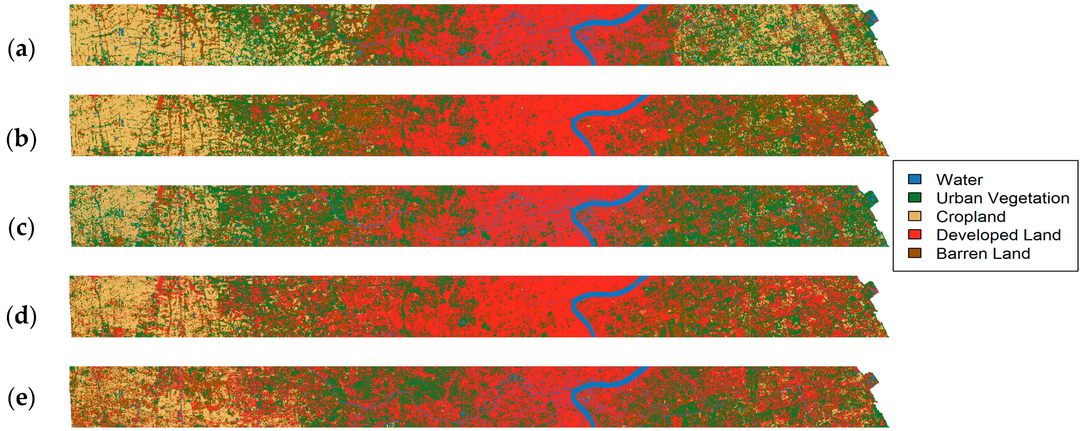
Figure 3.
Mean phenology model from multi-temporal Landsat images for a pixel of typical urban vegetation located in the east-west transect for the five periods: 1984–1995, 1996–2000, 2001–2005, 2006–2010, and 2011–2015. Each red point represents one Landsat image at the corresponding DOY. Green points indicate the spring onset (SOS) and the yellow points mark the fall senescence (EOS). The black lines show the fitted different logistic curves. The dashed lines are the first derivative of the fitted curves.
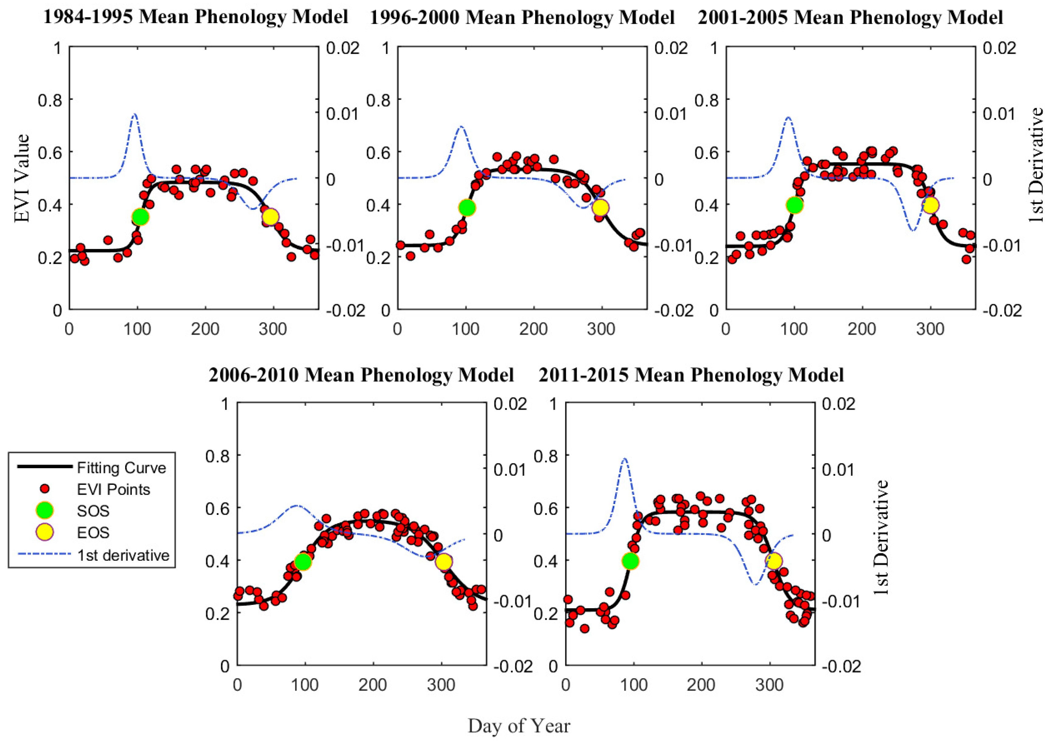
Figure 4.
Spatial pattern of mean SOS for urban vegetation along the east-west transect for the five periods: (a) 1984–1995; (b) 1996–2000; (c) 2001–2005; (d) 2006–2010 and (e) 2011–2015.
Figure 4.
Spatial pattern of mean SOS for urban vegetation along the east-west transect for the five periods: (a) 1984–1995; (b) 1996–2000; (c) 2001–2005; (d) 2006–2010 and (e) 2011–2015.
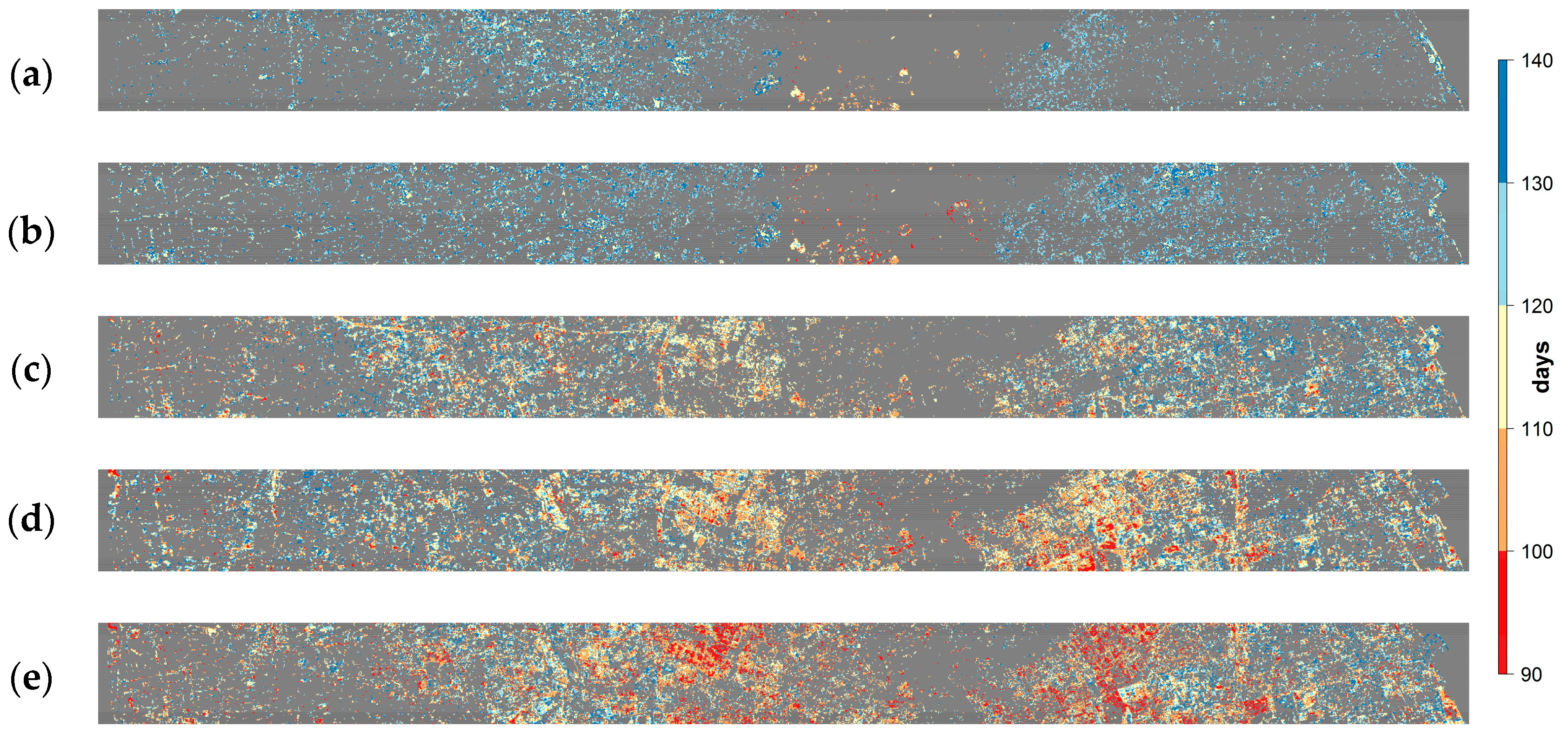
Figure 5.
Spatial pattern of the mean EOS for urban vegetation along the east-west transect for the five periods: (a) 1984–1995; (b) 1996–2000; (c) 2001–2005; (d) 2006–2010 and (e) 2011–2015.
Figure 5.
Spatial pattern of the mean EOS for urban vegetation along the east-west transect for the five periods: (a) 1984–1995; (b) 1996–2000; (c) 2001–2005; (d) 2006–2010 and (e) 2011–2015.
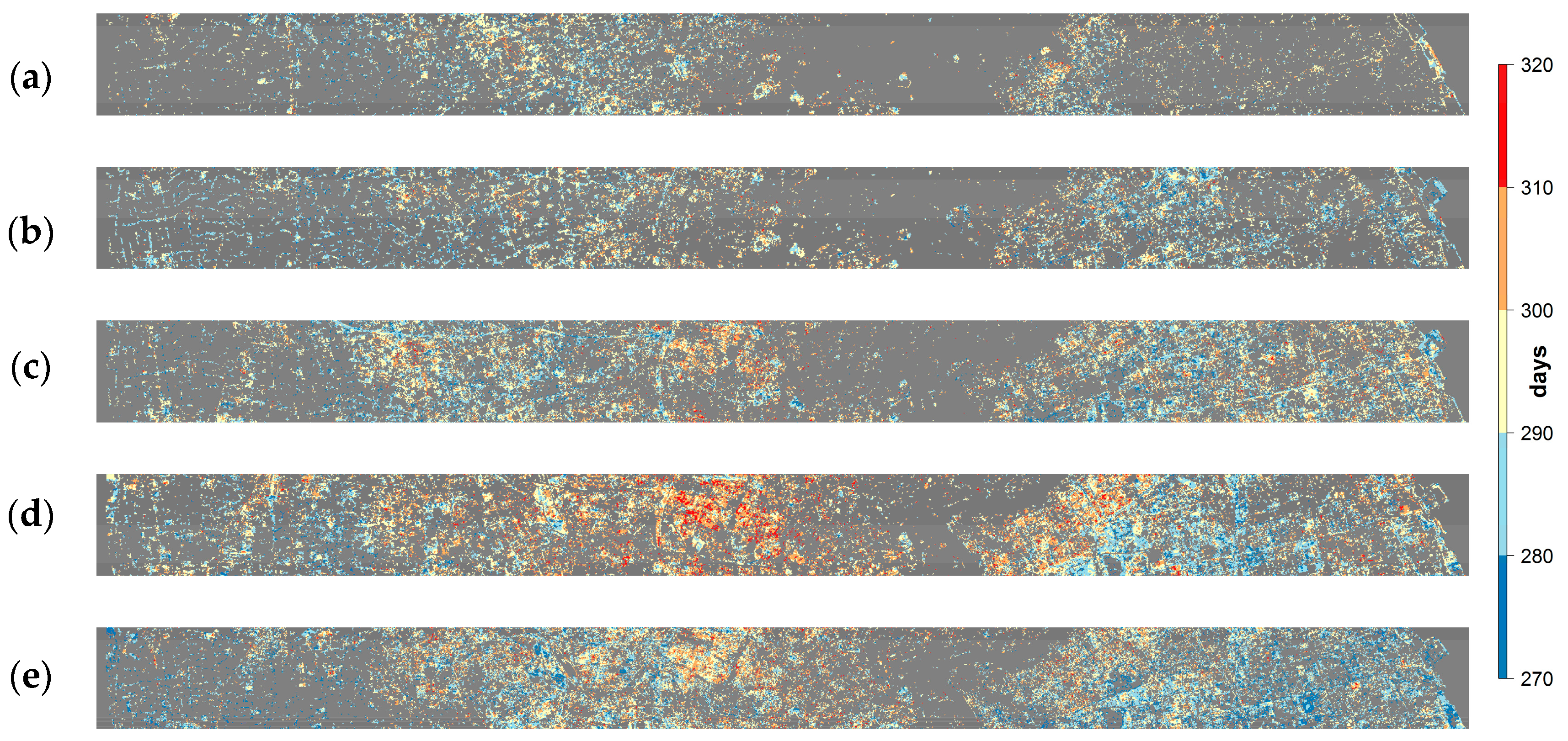
Figure 6.
Spatial pattern of the mean LOS for urban vegetation along the east-west transect for the five periods: (a) 1984–1995; (b) 1996–2000; (c) 2001–2005; (d) 2006–2010 and (e) 2011–2015.
Figure 6.
Spatial pattern of the mean LOS for urban vegetation along the east-west transect for the five periods: (a) 1984–1995; (b) 1996–2000; (c) 2001–2005; (d) 2006–2010 and (e) 2011–2015.
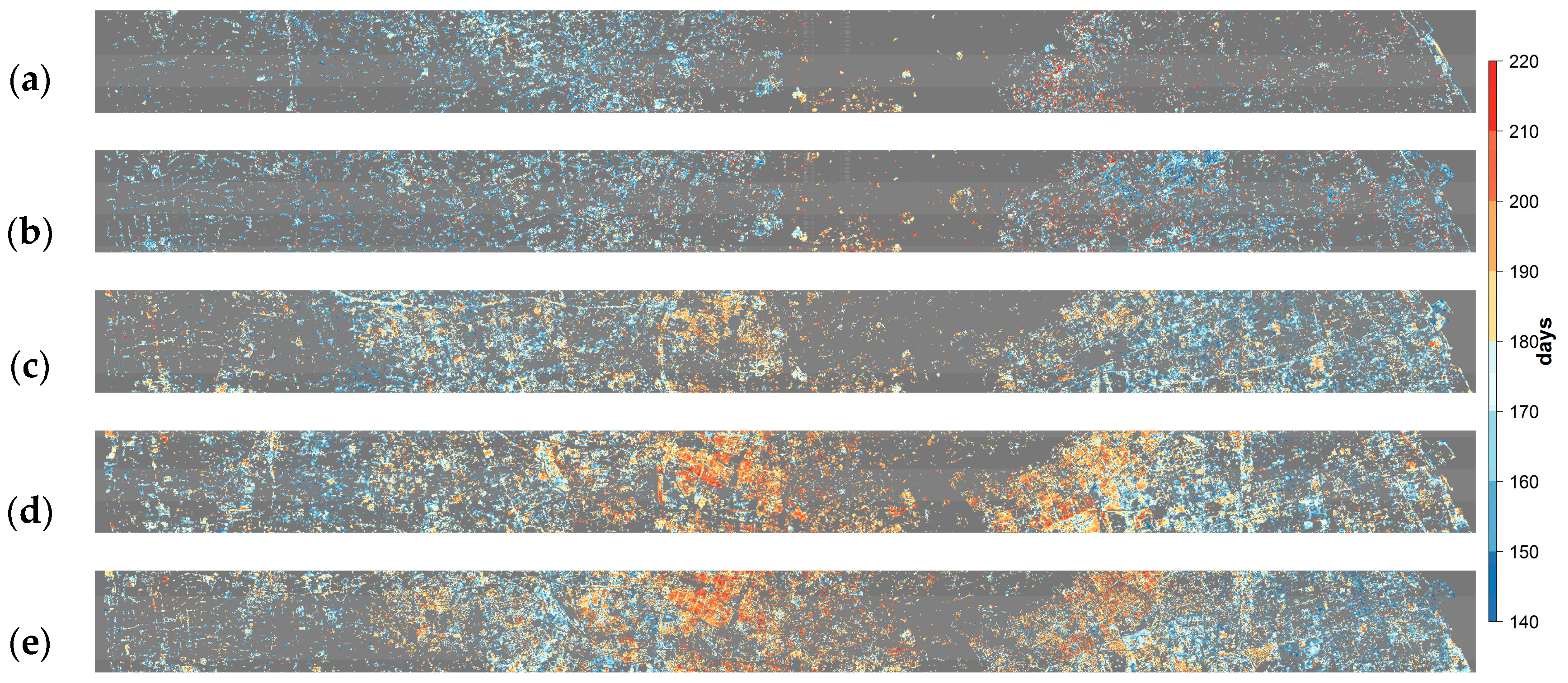
Figure 7.
Spatial mean SOS (a); EOS (b) and LOS (c) for urban vegetation as a function of distance along the east-west transect that runs through the urban center. The columns represent the periods: 1984–1995, 1996–2000, 2001–2005, 2006–2010, and 2011–2015. Bold lines represented average SOS, EOS, and LOS and shaded areas represented ± one standard deviation within each 5 km blocks.

Table 1.
Percentages of LCLU types in 2.5-m spatial resolution classification map.
| Year | RE(%) | PF (%) | IN (%) | TR (%) | VG (%) | WA (%) | AG (%) | OT (%) |
|---|---|---|---|---|---|---|---|---|
| 1994 | 19.65 | 3.17 | 12.58 | 5.66 | 10.93 | 8.86 | 36.04 | 3.11 |
| 2000 | 21.76 | 5.06 | 10.8 | 7.68 | 12.67 | 10.27 | 29.17 | 2.59 |
| 2005 | 21.84 | 5.97 | 13.97 | 9.34 | 14.29 | 9.19 | 20.33 | 5.07 |
Table 2.
Multi-season images used for LCLU classification with the AASG algorithm. The images for the year 1995 were classified separately and its LCLU map was used as reference map for AASG.
Table 2.
Multi-season images used for LCLU classification with the AASG algorithm. The images for the year 1995 were classified separately and its LCLU map was used as reference map for AASG.
| Year | Season | ||
|---|---|---|---|
| Early- | Mid- | Late- | |
| 1995 | DOY 92 (TM) | DOY 224 (TM) | DOY 304 (TM) |
| 2000 | DOY 86 (ETM+) | DOY 214 (ETM+) | DOY 310 (ETM+) |
| 2005 | DOY 67 (ETM+) | DOY 214 (2006, ETM+) | DOY 331 (TM) |
| 2010 | DOY 97 (ETM+) | DOY 244 (2011, ETM+) | DOY 313 (TM) |
| 2015 | DOY 100 (2014, OLI) | DOY 215 (OLI) | DOY 308 (2014, OLI) |
Table 3.
Landscape pattern metrics used in this study, after McGarigal et al. [51].
Table 3.
Landscape pattern metrics used in this study, after McGarigal et al. [51].
| Landscape Metrics | Definition |
|---|---|
| Composition metrics | |
| Percentage of Landscape area (PLAND) | PLAND quantifies the proportional abundance of each patch type in the landscape. |
| Shannon’s Diverversity Index (SHDI) | SHDI measures the diversity of LCLU types at the landscape level. |
| Shannon’s Evenness Index (SHEI) | SHEI measures the relative abundance of different patch types at landscape level. |
| Configuration metrics | |
| Patch Density (PD) | PD equals the number of patches of a given LCLU type in a landscape divided by its area. It is a measure of heterogeneity of the landscape. |
| Edge Density (ED) | ED is calculated as the sum of the lengths (m) of all edge segments involving a given patch type divided by the total landscape area. It is a measure of the shape complexity for a patch type in the landscape |
| Landscape Shape Index (LSI) | LSI provides a standardized measurement of total edges that adjusts for the size of the landscape. |
| Congtagion (CONTAG) | CONTAG quantifies both patch type interspersions as well as its spatial distribution. A smaller CONTAG value indicates higher interspersion and vice versa. It can only be calculated as a landscape level metric. |
| Clumpiness (CLUMPY) | CLUMPY ranges from −1 when a patch type is maximally disaggregated to 1 when the patch type is maximally aggregated. CLUMPY takes a value of zero for a patch type that is randomly distributed over the landscape. It can only be calculated as a class level metric. |
Table 4.
Percentages of LCLU types generated by AASG within the east-west transect.
| Year | Water (%) | Urban Vegetation (%) | Cropland (%) | Developed Land (%) | Barren Land (%) |
|---|---|---|---|---|---|
| 1995 | 7.24 | 19.77 | 31.12 | 35.91 | 5.96 |
| 2000 | 7.49 | 23.13 | 23.99 | 38.61 | 6.78 |
| 2005 | 8.75 | 25.31 | 19.5 | 41.11 | 5.33 |
| 2010 | 7.91 | 24.22 | 15.77 | 45.09 | 7.01 |
| 2015 | 7.65 | 22.12 | 14.92 | 48.32 | 6.99 |
Table 5.
Percentages of longer LOS, shorter LOS, and no-change of LOS within the east-west transect for the five time periods.
Table 5.
Percentages of longer LOS, shorter LOS, and no-change of LOS within the east-west transect for the five time periods.
| Time Period | Shorter LOS (%) | Longer LOS (%) | No-Change (%) |
|---|---|---|---|
| 1984–1995 | 38.04 | 12.59 | 49.37 |
| 1996–2000 | 39.54 | 10.38 | 50.08 |
| 2001–2005 | 11.33 | 13.22 | 75.45 |
| 2006–2010 | 3.87 | 36.31 | 59.82 |
| 2011–2015 | 8.60 | 22.18 | 69.22 |
Table 6.
Pearson correlation coefficients between SOS, EOS, and LOS of urban vegetation and landscape level pattern metrics for the time periods of 1984–1995, 1996–2000, and 2001–2005, respectively.
Table 6.
Pearson correlation coefficients between SOS, EOS, and LOS of urban vegetation and landscape level pattern metrics for the time periods of 1984–1995, 1996–2000, and 2001–2005, respectively.
| Landscape Metrics | 1984–1995 | 1996–2000 | 2001–2005 | ||||||
|---|---|---|---|---|---|---|---|---|---|
| SOS | EOS | LOS | SOS | EOS | LOS | SOS | EOS | LOS | |
| PD | −0.021 | −0.372 | −0.155 | 0.684 *** | −0.615 *** | −0.672 *** | 0.74 *** | −0.412 * | −0.706 *** |
| ED | −0.378 | 0.461 * | 0.492 * | 0.381 | −0.348 | −0.377 | 0.703 *** | −0.213 | −0.599 ** |
| LSI | −0.415 * | 0.441 * | 0.511 ** | 0.371 | −0.341 | −0.368 | 0.708 *** | −0.208 | −0.601 ** |
| CONTAG | 0.412 * | −0.594 ** | −0.579 ** | 0.612 *** | −0.496 ** | −0.576 ** | −0.31 | −0.229 | 0.135 |
| SHDI | −0.372 | 0.563 ** | 0.535 ** | −0.681 *** | 0.567 ** | 0.649 *** | 0.243 | 0.24 | −0.082 |
| SHEI | −0.384 | 0.574 ** | 0.549 ** | −0.681 *** | 0.559 ** | 0.645 *** | 0.18 | 0.282 | −0.018 |
Significance levels (two-tailed): *** 0.001, ** 0.01, * 0.05.
Table 7.
Pearson correlation coefficients between SOS, EOS, and LOS of urban vegetation and class level landscape metrics for time intervals 1984–1995, 1996–2000, and 2001–2005. The last two letters after each landscape metric signify the LCLU type as defined in Section 2.2.
Table 7.
Pearson correlation coefficients between SOS, EOS, and LOS of urban vegetation and class level landscape metrics for time intervals 1984–1995, 1996–2000, and 2001–2005. The last two letters after each landscape metric signify the LCLU type as defined in Section 2.2.
| Landscape Metrics | 1984–1995 | 1996–2000 | 2001–2005 | ||||||
|---|---|---|---|---|---|---|---|---|---|
| SOS | EOS | LOS | SOS | EOS | LOS | SOS | EOS | LOS | |
| PLAND_RE | −0.692 *** | 0.743 *** | 0.856 *** | −0.864 *** | 0.844 *** | 0.881 *** | −0.722 *** | 0.805 *** | 0.85 *** |
| PD_RE | 0.115 | −0.039 | −0.104 | 0.538 ** | −0.486 * | −0.53 ** | 0.19 | −0.167 | −0.206 |
| ED_RE | −0.621 *** | 0.718 *** | 0.791 *** | −0.592 ** | 0.559 ** | 0.594 ** | −0.588 ** | 0.768 *** | 0.737 *** |
| LSI_RE | −0.301 | 0.276 | 0.35 | 0.469 * | −0.448 * | −0.473 * | 0.243 | −0.111 | −0.222 |
| CLUMPY_RE | −0.062 | 0.238 | 0.155 | −0.74 *** | 0.709 *** | 0.747 *** | −0.366 | 0.437 * | 0.442 * |
| PLAND_PF | −0.699 *** | 0.707 *** | 0.844 *** | −0.814 *** | 0.703 *** | 0.787 *** | −0.679 *** | 0.554 ** | 0.718 *** |
| PD_PF | −0.657 *** | 0.656 *** | 0.79 *** | −0.74 *** | 0.627 *** | 0.71 *** | −0.668 *** | 0.476 * | 0.679 *** |
| ED_PF | −0.691 *** | 0.696 *** | 0.833 *** | −0.783 *** | 0.681 *** | 0.759 *** | −0.694 *** | 0.538 ** | 0.723 *** |
| LSI_PF | −0.695 *** | 0.668 *** | 0.823 *** | −0.828 *** | 0.746 *** | 0.815 *** | −0.682 *** | 0.585 ** | 0.733 *** |
| CLUMPY_PF | 0.727 *** | −0.398 * | −0.724 *** | −0.139 | 0.302 | 0.218 | 0.355 | −0.128 | −0.311 |
| PLAND_IN | −0.639 *** | 0.54 ** | 0.723 *** | −0.5 ** | 0.581 ** | 0.552 ** | 0.236 | 0.182 | −0.099 |
| PD_IN | −0.716 *** | 0.495 * | 0.76*** | −0.143 | 0.252 | 0.198 | 0.437 * | −0.123 | −0.369 |
| ED_IN | −0.705 *** | 0.614 *** | 0.806 *** | −0.442 * | 0.555 ** | 0.507 ** | 0.327 | 0.098 | −0.2 |
| LSI_IN | −0.684 *** | 0.626 *** | 0.796 *** | −0.254 | 0.386 | 0.323 | 0.392 * | −0.022 | −0.295 |
| CLUMPY_IN | 0.359 | 0.026 | −0.255 | −0.633 *** | 0.573 ** | 0.624 *** | −0.016 | 0.161 | 0.076 |
| PLAND_TR | −0.732 *** | 0.645 *** | 0.84*** | −0.912*** | 0.794*** | 0.885*** | −0.663 *** | 0.655 *** | 0.747 *** |
| PD_TR | 0.01 | −0.605 ** | −0.284 | 0.779*** | −0.677*** | −0.755*** | 0.791 *** | −0.552 ** | −0.799 *** |
| ED_TR | −0.815 *** | 0.589 ** | 0.876 *** | −0.824 *** | 0.689 *** | 0.786 *** | −0.557 ** | 0.649 *** | 0.666 *** |
| LSI_TR | −0.837 *** | 0.311 | 0.766 *** | −0.025 | −0.067 | −0.017 | 0.179 | 0.045 | −0.112 |
| CLUMPY_TR | −0.08 | 0.365 | 0.226 | −0.902 *** | 0.826 *** | 0.894 *** | −0.49* | 0.602** | 0.599** |
| PLAND_VG | −0.409 * | 0.28 | 0.433 * | −0.327 | 0.182 | 0.27 | −0.042 | 0.016 | 0.037 |
| PD_VG | 0.047 | −0.656 *** | −0.335 | 0.818 *** | −0.777 *** | −0.823 *** | 0.711 *** | −0.404 * | −0.681 *** |
| ED_VG | −0.008 | −0.574 ** | −0.257 | 0.306 | −0.387 | −0.353 | 0.772 *** | −0.514 ** | −0.77 *** |
| LSI_VG | 0.125 | −0.732 *** | −0.428 * | 0.802 *** | −0.82 *** | −0.834 *** | 0.799 *** | −0.616 *** | −0.831 *** |
| CLUMPY_VG | −0.253 | 0.745 *** | 0.529 ** | −0.884 *** | 0.882 *** | 0.909 *** | −0.661 *** | 0.61 *** | 0.727 *** |
| PLAND_WA | 0.595 ** | −0.363 | −0.609 *** | 0.472 * | −0.502 ** | −0.5 ** | 0.498 ** | −0.418 * | −0.531 ** |
| PD_WA | 0.577 ** | −0.253 | −0.546 ** | 0.394 * | −0.447 * | −0.43 * | 0.804 *** | −0.344 | −0.725 *** |
| ED_WA | 0.818 *** | −0.495 * | −0.836 *** | 0.731 *** | −0.632 *** | −0.707 *** | 0.853 *** | −0.497 ** | −0.822 *** |
| LSI_WA | 0.7 *** | −0.457 * | −0.73 *** | 0.734 *** | −0.636 *** | −0.711 *** | 0.833 *** | −0.466 * | −0.796 *** |
| CLUMPY_WA | −0.545 ** | 0.351 | 0.566 ** | −0.625 *** | 0.518 ** | 0.594 ** | −0.694 *** | 0.306 | 0.63 *** |
| PLAND_AG | 0.668 *** | −0.713 *** | −0.824 *** | 0.922 *** | −0.857 *** | −0.92 *** | 0.485 * | −0.689 *** | −0.63 *** |
| PD_AG | 0.688 *** | −0.58 ** | −0.778 *** | 0.695 *** | −0.562 ** | −0.654 *** | 0.833 *** | −0.499 ** | −0.808 *** |
| ED_AG | 0.746 *** | −0.664 *** | −0.859 *** | 0.85 1*** | −0.774 *** | −0.841 *** | 0.734 *** | −0.641 *** | −0.793 *** |
| LSI_AG | 0.72 *** | −0.629 *** | −0.824 *** | 0.75 *** | −0.691 *** | −0.745 *** | 0.845 *** | −0.586 ** | −0.852 *** |
| CLUMPY_AG | 0.211 | −0.204 | −0.251 | −0.878 *** | 0.824 *** | 0.879 *** | 0.292 | −0.288 | −0.329 |
| PLAND_OT | 0.006 | 0.392 * | 0.175 | −0.553 ** | 0.382 | 0.491 * | 0.263 | 0.024 | −0.183 |
| PD_OT | −0.674 *** | 0.779 *** | 0.859 *** | −0.794 *** | 0.672 *** | 0.762 *** | −0.034 | 0.29 | 0.141 |
| ED_OT | −0.423 * | 0.665 *** | 0.619 *** | −0.685 *** | 0.534 ** | 0.636 *** | 0.233 | 0.089 | −0.135 |
| LSI_OT | −0.621 *** | 0.737 *** | 0.8 *** | −0.742 *** | 0.636 *** | 0.715 *** | 0.071 | 0.272 | 0.057 |
| CLUMPY_OT | 0.749 *** | −0.555 ** | −0.812 *** | −0.219 | 0.258 | 0.243 | 0.412* | −0.135 | −0.355 |
Significance levels (two-tailed): *** 0.001, ** 0.01, * 0.05.
© 2017 by the authors. Licensee MDPI, Basel, Switzerland. This article is an open access article distributed under the terms and conditions of the Creative Commons Attribution (CC BY) license (http://creativecommons.org/licenses/by/4.0/).
Share and Cite
MDPI and ACS Style
Qiu, T.; Song, C.; Li, J. Impacts of Urbanization on Vegetation Phenology over the Past Three Decades in Shanghai, China. Remote Sens. 2017, 9, 970. https://doi.org/10.3390/rs9090970
AMA Style
Qiu T, Song C, Li J. Impacts of Urbanization on Vegetation Phenology over the Past Three Decades in Shanghai, China. Remote Sensing. 2017; 9(9):970. https://doi.org/10.3390/rs9090970
Chicago/Turabian StyleQiu, Tong, Conghe Song, and Junxiang Li. 2017. "Impacts of Urbanization on Vegetation Phenology over the Past Three Decades in Shanghai, China" Remote Sensing 9, no. 9: 970. https://doi.org/10.3390/rs9090970
Note that from the first issue of 2016, this journal uses article numbers instead of page numbers. See further details here.