Modeling Self-Assembly Across Scales: The Unifying Perspective of Smart Minimal Particles

Abstract

A wealth of current research in microengineering aims at fabricating devices of increasing complexity, notably by (self-)assembling elementary components into heterogeneous functional systems. At the same time, a large body of robotic research called swarm robotics is concerned with the design and the control of large ensembles of robots of decreasing size and complexity. This paper describes the asymptotic convergence of micro/nano electromechanical systems (M/NEMS) on one side, and swarm robotic systems on the other, toward a unifying class of systems, which we denote Smart Minimal Particles (SMPs). We define SMPs as mobile, purely reactive and physically embodied agents that compensate for their limited on-board capabilities using specifically engineered reactivity to external physical stimuli, including local energy and information scavenging. In trading off internal resources for simplicity and robustness, SMPs are still able to collectively perform non-trivial, spatio-temporally coordinated and highly scalable operations such as aggregation and self-assembly (SA). We outline the opposite converging tendencies, namely M/NEMS smarting and robotic minimalism, by reviewing each field's literature with specific focus on self-assembling systems. Our main claim is that the SMPs can be used to develop a unifying technological and methodological framework that bridges the gap between passive M/NEMS and active, centimeter-sized robots. By proposing this unifying perspective, we hypothesize a continuum in both complexity and length scale between these two extremes. We illustrate the benefits of possible cross-fertilizations among these originally separate domains, with specific emphasis on the modeling of collective dynamics. Particularly, we argue that while most of the theoretical studies on M/NEMS SA dynamics belong so far to one of only two main frameworks—based on analytical master equations and on numerical agent-based simulations, respectively—alternative models developed in swarm robotics could be amenable to the task, and thereby provide important novel insights.

1. Introducing Smart Minimal Particles

Distributed Systems (DSs) are ensembles of elements (hereby referred to as particles for the sake of generality) spatially scattered within bounded domains, and whose collective properties depend on those of the elements and of their interactions, both with each other and with the environment. DSs come in several varieties, depending on, e.g., their coordination and control strategies (centralized versus de-centralized), availability and sharing of resources (internal or external, global or local, including information and energy), constraints, tasks, performance and adaptivity—besides the specific characteristics of the elements and interactions. Biology at large is the prime source of examples of DSs and self-organization [1]. Their potentialities have in turn inspired the introduction of DSs in broad fields of intensive research and increasing technological pervasiveness such as, among others, distributed information processing (e.g., Internet and cloud computing, wireless communications and sensor networks [2]), micro/nano electromechanical systems (M/NEMS) [3] and artificial intelligent systems [4]. The latter two fields are of particular interest in our view, because they represent the extremes of the complexity and size continuum of artificial distributed systems and, at the same time, they manifest a convergence towards a shared, conceptual and technological midpoint, embodied by what we hereby denote Smart Minimal Particles (SMPs) (Figure 1).

On one side of the continuum, robotic agents are normally macroscopic (i.e., from a few millimeters to a few tens of centimeters in size), autonomous in terms of energy, locomotion and communication, and they can be described by a (finite) number of internal states that determine their deliberative response to environmental influences. However, autonomy comes at the price of high complexity (Complexity and simplicity refer herein to a measure of the sophistication of internal resources.), cost, and susceptibility to failure. Therefore, a very active research topic in robotics concerns the design and control of massively-distributed robotic systems involving simpler and smaller robots. Such swarm robotic systems generally exploit self-organization, redundancy and environmental surrogates to compensate for the technological limitations of the individual robots (e.g., fluid flows for mass transport [5], stigmergy [6,7], templating [8]). This approach is consistent with the more general minimalist trend of robotics [9]. While the required miniaturization of robotic modules is a difficult task in itself, a contextual challenge for minimalism (as defined earlier) is the design of simpler and more robust agents still capable of performing desired cooperative tasks in noisy environments and in spite of technological limitations. By minimizing the number of their internal states—besides their communication, sensing, and actuation capabilities, and their mobility—these robotic agents tend to asymptotically approach the status of purely reactive agents, just like molecules, bacteria, or M/NEMS.

On the other side of the continuum, an important body of precision manufacturing's research aims at producing very-small systems of increasing complexity. One promising route to fabricate complex functional systems is the autonomous self-organization and buildup of structures from their simpler subunits. As a prominent example, active and passive M/NEMS devices come in large quantities owing to batch fabrication technologies [10], but their organized integration into heterogeneous functional systems by means of serial manipulation, as done in e.g., consumer electronic manufacturing, is limited in terms of throughput, flexibility, and scalability [11]. Therefore, massively parallel and high-throughput integration is invoked, as embodied by bottom-up methods such as e.g., self-assembly (described in Section 2). However, specific geometric design and surface derivatization are required to enable the accurate and efficient self-assembly of M/NEMS devices into desired, articulated structures. Such dedicated physico-chemical tailoring encodes local information and selective interactions to direct the cooperative aggregation. We denote smarting this tendency toward an increased sophistication of M/NEMS devices, and of passive particles (defined in Section 2) in general. Conceptually, smarting is the opposite of minimalism: in a nutshell, minimalism tends to make intelligent particles as simple, reactive and passive as possible, while smarting tends to make passive particles as complex, deliberative and active as possible.

In our view, smart minimal particles (SMPs) represent the natural convergence locus of such opposing tendencies observed in M/NEMS technology and swarm robotics.

We define SMPs as mobile, sub-millimeter sized, purely reactive agents that compensate their lack of on-board resources with their specifically engineered reactivity to external physical stimulation as well as ability to scavenge energy and information from their local environment. SMPs may be subject to both global and local physical influences, yet they are only capable of local interactions. Influences on SMPs can derive from specific stimuli (e.g., wireless actuation by frequency-selective magnetic induction [12]), interaction potentials [13] or field gradients (e.g., gravitational, electric, magnetic, temperature, pressure), also programmable (e.g., mechanical [14], electric [15]). A partial list of examples of application-specific particle engineering includes: selective hydrophobic or -philic surface functionalization [16]; steric affinities based on shape-complementary or matching particle/binding site geometries [17,18]; selective coating with fluids of high interfacial energies, such as polymers [19,20] or molten solders [21]; magnetic [22] and electric polarizations, both electrostatic [23] and electrodynamic [24]; DNA-based derivatization [25,26]. States of SMPs are associated with interfacial conformational switchings [27], i.e., with the modification of their chemical and/or mechanical interface with the environment, as a consequence of, e.g., global stimuli [25], interactions with other particles or with templates (e.g., proximity-dependent activation [28], memory of individual assembly history [29]), or modification in the local properties of the environment (e.g., solution pH and light intensity [30]). SMPs trade off internal resources for simplicity and robustness, and are still able to perform non-trivial collective operations exploiting local interactions; eminently, spatio-temporally coordinated, decentralized and scalable organization—i.e., aggregation and, particularly, self-assembly.

SMPs blur the boundary between M/NEMS and swarm robotics by pointing toward an ideal continuum in particle size and complexity levels—from passive to active particles. Contextually, they also suggest the possibility of fruitful cross-fertilizations, i.e., the adoption in one domain of terminology and modeling frameworks originally developed in the other domain.

In this paper, we argue the need for and the proposal of SMPs (i) by outlining the mentioned convergence toward SMPs with experimental and theoretical examples drawn from both the M/NEMS' and modular robotics' literature on self-assembly and aggregation, (ii) by illustrating our suggested SMP perspective with specific respect to the modeling of the dynamics of self-assembling SMPs, and (iii) by adopting a shared, hybrid terminology where possible.

The paper is structured as follows. Section 2 briefly illustrates the varieties of self-assembly possible at most scales before specifically focusing on its static type as the most pertinent to SMPs (though far from exhausting their potentialities). Examples are drawn from both the modular robotics (Section 2.1) and the M/NEMS literature (Section 2.2); quasi-statics, transient dynamics and collective dynamics of self-assembly are also discussed (Section 2.3). The collective dynamics of SMPs is then addressed in detail in Sections 3 and 4, which critically review the main, sometimes analogous models proposed so far for passive particles—i.e., master equation-based (Section 3.1) and agent-based models (Section 3.2)—and for active particles—i.e., stochastic reaction models (Section 4.1) and hybrid automata (Section 4.2)—respectively. These reviews prelude to an outline of a proposed, unifying modeling framework for SMPs, namely multi-level modeling (Section 5), which integrates a set of conceptually-different models, ranked according to their level of abstraction and stacked into a coherent hierarchical system across which control and design parameters can be seamlessly transferred from one model to the other, either upward (i.e., abstraction) or downward (i.e., implementation). Finally, Section 6 presents concluding remarks and perspectives for future research.

2. Self-Assembly across Scales

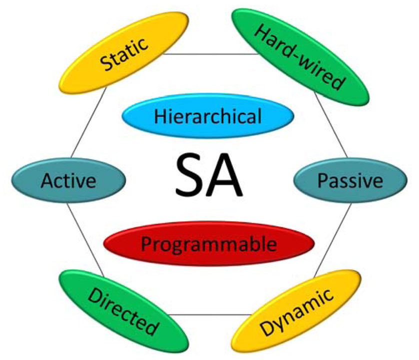
Self-assembly (SA) [31] has recently gained considerable momentum in the realm of precision engineering and manufacturing [32,33]. Particularly, SA represents the main embodiment of the bottom-up approach to the fabrication of heterogeneous and articulated micro-and nanosystems [34]. Rooted in, and constantly inspired by, biology and supermolecular chemistry [35], such an approach is complementary to the top-down fabrication approach established at (though not exclusive to) the macroscale because of its highly decentralized, massively parallel, and largely unsupervised control [11], which, together with intrinsic redundancy, makes it also highly robust [36] and, in principle, scalable to the control of larger structures. Interestingly, combinations of both approaches are being currently envisioned, as in e.g., hybrid microhandling [37,38]. A taxonomy of SA is sketched in Figure 2.

In its static templated (or directed) variety—commonly adopted for M/NEMS coordinated aggregation, and main focus of this contribution—SA builds up ordered structures out of biased stochastic searches within bounded assembly spaces and over the free energy landscapes of the assembling systems. The characteristics of these landscapes can be specified by the physicochemical features of the particles to be assembled, their mutual interactions, and their reactivity to external stimuli and to the boundary conditions (including templating) imposed by the assembly space. All of these elements can be tailored to control the assembly process. Indeed, the interplay between biases and stochasticity—object of an ongoing debate in SA-based manufacturing—enables SA's extensive flexibility and effective search in solution or assembly space; very similar mechanisms are harnessed in a large class of stochastic optimization algorithms (e.g., simulated annealing [39], stochastic gradient descent [40]) used for solving constraint-satisfaction problems. By embedding randomness, SA is intrinsically robust against noise, deadlocks and locally optimal points; using seeds and biases, the progress of SA is purposely directed. Particularly, templating is exploited in a vast class of SA processes of eminent importance for industrial manufacturing, where time-to-assembly and throughput are normally critical performance metrics. In this context, the introduction of pre-designed physical templates with target binding sites, of selective (an)isotropic affinities, and of complementary shape-matching geometries enable (globally and locally, respectively) the growth of predictable structures and the enhancement of their assembly rates. Besides, in some SA instances the spatial and/or temporal sequence of assembly events can be pre-programmed to a certain extent [41-43]; also, the assembling particles can in turn be the result of prior SA of simpler particles (hierarchical SA) [44].

More importantly, SA processes can be broadly classified according to the role played by energy and to the level of pro-activity of the particles to achieve aggregation [31]. As for the former classification, in static SA (sSA) processes energy is dissipated only while the assembling system is approaching (possibly, one of) its minimal energy configuration(s). In sSA the thermodynamic concept of free energy landscape can be applied, and there is no further action by nor energy release from the system once the system has reached equilibrium. Conversely, in dynamic SA (dySA) [45] the sustained energy dissipation itself is the origin of the organization of ordered, steady-state spatio-temporal patterns of particles. DySA emerges in systems driven out of thermodynamic equilibrium (e.g., dissipative structures [46]) by the constant exposure to an external energy gradient. The implied structural organization is thought to underlie most biological phenomena [47]. Significant researches toward a comprehensive theory of DySA, still missing, are being pursued (see e.g., [48,49]). Concerning the latter classification, the particles can (active SA) or cannot (passive SA) purposely expend internal resources (e.g., energy, communication) to drive the process or establish selective physical or informational links with other particles. Active particles(An active particle is also active in the electric (device) meaning of the term, though the opposite is not necessarily true: e.g., electrically-active M/NEMS are normally passive for SA purposes.) can be identified with agents endowed with degrees of autonomy and with internal states(Hard-wired SA encodes the sequence of assembly events in the states of the particles. Examples range from living cells [50] to self-replicating artificial structures [51].), able to make choices (regarding e.g., trajectories, links to other particles). Instead, in passive particles the autonomy is strictly limited to scavenging means of mass transport from the environment, conformational switchings, and to the compliance with the physical interactions as mediated by body and surface forces.

In the following sections, recent results concerning experimental and modeling SA activities in robotics and M/NEMS are reviewed.

2.1. Self-Assembly of Small Modular Robots

Achieving SA and aggregation are important tasks in distributed and modular robotics [52], as supported by a vast literature, both theoretical and experimental.

Probabilistic models were developed for the aggregation and SA of mobile robots [53,54], along with deterministic models of aggregation and flocking (i.e., the coordinated motion of the aggregates) [55,56], and graph-based approaches [57]. A comprehensive theoretical study of microscopic robot coordination in viscous fluids was carried out by Hogg [58]. Stochastic and distributed control of swarms of robots was extensively studied by Kumar and colleagues [59], who also exploit modeling methods originating from the study of chemical systems [60]. The chemical formalism well suits the description of SA, as will be shown in Sections 3.1 and 4.1 and as further demonstrated in recent studies involving real and simulated robots [61,62].

Aggregation of passive objects mediated by mobile robots [7], self-organized aggregation of mobile robots [63,64] and even of robots and insects [65] was extensively investigated using very diverse robotic platforms, ranging from a few to several centimeters in size [66]. Actual SA was achieved on the Swarm-bot, a 15 cm-sized mobile robot equipped with a gripper [67], and with Klavins' programmable parts, i.e., triangular robots (12.5 cm in size) that randomly slide on an air table and assemble with each other according to pre-planned schemes ([53], see also Section 4.1). Miyashita et al. proposed simpler triangular robots (Tribolons, 4.9 cm in size) that assemble with each other at the water/air interface and rely on a pantograph for both energy supply and control [68].

SA of sub-centimeter sized robots is also being addressed. Donald et al. demonstrated MEMS robots (i.e., miniature robots fabricated by micromachining) that can selectively respond to a single, global control signal delivered through the interdigitated electrodes of an insulated substrate [69]. Thanks to their scratch-drive actuator and single steering arm, such robots can describe intersecting trajectories and dock compliantly together, forming planar structures several times their own size. Frutiger et al. fabricated sub-millimetric MEMS robots that utilize a wireless resonant magnetic microactuator to get power supply, achieve propulsion and perform servoed exploration and possibly cooperative tasks [12]. Such Magmites convert the energy of magnetic fields into mechanical motion directly, and can be controlled by frequency-coded signals. Chang et al. demonstrated the electro-osmotic motion of millimetric, light-responsive diodes controlled by an external AC electric field [70]. Several research groups envision designing modular surgical robots small enough (about 1 cm) for entering the human body through natural orifices (e.g., by ingestion [71]) and capable of configuring themselves into kinematic structures within the stomach. Further examples are referred to in [12].

Consistently with our SMP perspective, the ongoing miniaturization of robotic modules may thus further decrease the gap, both in size and performance, with M/NEMS—whose SA is reviewed next.

2.2. Self-Assembly of M/NEMS

For the assembly of micro- and nanosystems, a wealth of static templated SA processes were proposed and demonstrated, as detailed in several recent reviews [3,33,34]. A very wide range of applications is targeted, including, e.g., three-dimensional electric circuits [72], flexible LED-based displays [42], integration of semiconductor devices onto plastic substrates [17], polyhedral containers [33], monocrystalline solar cells [16]. They exploit a broad spectrum of physical interactions, including (but not limited to) gravitational [73], hydrophobic [74], steric [18], electric [24], magnetic [22], capillary [75], DNA hybridization-mediated [25], fluidic [76]. Interestingly, in the range of micrometric to nanometric scales most of these interactions can be tuned to a reasonable degree [35,77]. Unless an adaptive system is required [45], the static type of SA is adopted here because of the functional and disposable nature of the systems themselves(Reconfigurable systems (e.g., by disassembly) are also hereby included, as they can be thought of as a sequence of static SA processes, each starting from the pre-configuration left from the previous instance). As for the M/NEM units, in practically all cases they are only required to be able to scavenge energy and information from the environment (particularly, from templates and other parts) and to recognize their target position in the assembling structures. For this purpose, they need proper pre-conditioning, outlined in Section 1.

2.3. Modeling Static Self-Assembly

SA entails several correlated phenomena at different levels of detail—each being possibly subject to modeling. Models of sSA of passive particles mainly focus on three main aspects: quasi-statics, transient dynamics and collective dynamics (There is no contradiction here: the dynamics refers here to the transient approach—at single and collective particle level, respectively—to the static (final) system configuration). The first two aspects concern the highly accurate, case-specific modeling of material, physico-chemical, and geometrical properties influencing the SA performance of a single particle in relatively-close proximity to its (optimal) target position in the assembling structure. The latter, complementary aspect concerns a more relational, multi-particle perspective which, while reducing accuracy by sparing a substantial amount of details about the physical and geometrical details of the system, still captures meaningful information about the cooperativity of the process and possibly gains in generality and computational efficiency.

Analytical models (based on first-order approximations and/or first-principles equations) and finite-element numerical simulations, often coupling multiple physical domains, well suit physical modeling. Due to scaling laws, the hierarchy of magnitudes of physical forces at sub-millimetric scales, where surface phenomena dominate, is different from that at the macroscale [78]; this favors different actuation and interaction mechanisms at different scales. A substantial amount of rather case-specific works addressed both quasi-statics (see e.g., [79-82] and references therein) and transient dynamics (see e.g., [83,84] and references therein).

Statistical mechanics is the discipline most devoted to the probabilistic modeling of large ensembles of particles and their collective properties, including their dynamics [85]. However, up to now M/NEMS and particularly robotic ensembles considered far lower counts of particles, which should in principle be treated by specific thermodynamics [34]. To date, very little effort has been dedicated to the modeling of passive particles' collective dynamics (see Section 3). We believe that this is due to: (1) the prominence, in the M/NEMS community, of the fully-fledged physical modeling of single particle's behavior as opposed to the modeling of collective dynamics; (2) the ability of the existing models to reasonably predict qualitative assembly trends; more importantly, (3) the lack of multi-objective cost functions in the proposed SA applications (mainly industrial manufacturing), which were mostly interested in optimizing throughput and/or time-to-assembly; and, possibly, (4) a lack of knowledge of modeling frameworks developed in other domains such as swarm robotics. The convergence of M/NEMS toward SMPs (Section 1) could also help in significantly shrinking this gap.

3. Modeling the SA Dynamics of Passive Particles

The main models of the SA dynamics of passive particles proposed in literature belong to one of two general approaches, namely: (1) analytical, rate equation-based, and (2) numerical, agent-based. They are illustrated and exemplified in the following sections.

3.1. Master Equation-Based Models

A master equation is a set of equations describing the probability distribution with which a given system S occupies each state i of its discrete set of states S. It can be put in the generic form:

$$N_i(t+\mathrm{\Delta }t)-N_i(t)=\sum _{i\ne j}\left\{p\left[i(t+\mathrm{\Delta }t)|j(t)\right]\cdot N_j(t)-p\left[j(t+\mathrm{\Delta }t)|i(t)\right]\cdot N_i(t)\right\}$$

(1)

where N_i is the number of system elements in state i, and p(i(t + Δt)∣j(t)) = p_ij is the conditional transition probability from state j to state i within the time interval Δt (∀i, j ⊂ S). The first (second) term of the right-end side of Equation 1 describes the inflow (outflow) of elements for state i. For a finite (infinitesimal) value of Δt, Equation 1 takes the form of a first-order finite-difference (differential) equation, as shown in Equation 2 (Equation 3):

$$N_i(t+1)-N_i(t)=\sum _{i\ne j}\left[p_{ij}\cdot N_j(t)-p_{ji}\cdot N_i(t)\right]$$

(2)

$$\frac{d{N}_i(t)}{dt}=\sum _{i\ne j}\left[k_{ij}\cdot N_j(t)-k_{ji}\cdot N_i(t)\right]$$

(3)

where k_ij is the transition rate from state j to state i. Equation 3 is also called rate equation.

The master equation derives from a deterministic description of Markov processes, which are memoryless stochastic processes in continuous time (i.e., where the state at time t contains all the information necessary to determine states at time t′> t )(The Markov property pertains to the model, not necessarily to the described system). Markov processes have proven extremely successful for modeling a large variety of dynamical systems [86].

Very common in statistical physics and chemistry, master equations were also adopted in models of the collective dynamics of smart particles. Before introducing the latter models, we shall review their most fundamental assumptions (we denote reactions both assembly and disassembly events).

• The system is well-mixed (or -stirred): all particles have equal probability to be at any point in space at any time. Accordingly, a given particle has equal probability to encounter any other particle or binding site at any time.

• The reactions are independent: the (dis)assembly of one particle does not affect the probability of (dis)assembly of other particles.

• The reaction probabilities are time-invariant and independent on the number of particles and sites. Accordingly, assembly at one site does not affect the availability of any other site for assembly, nor its probability of being filled.

• Only bi-particle events are considered, both for assembly (producing dimers) and disassembly.

Such assumptions are discussed in Section 3.1.4.

3.1.1. Hosokawa's State Variable Model

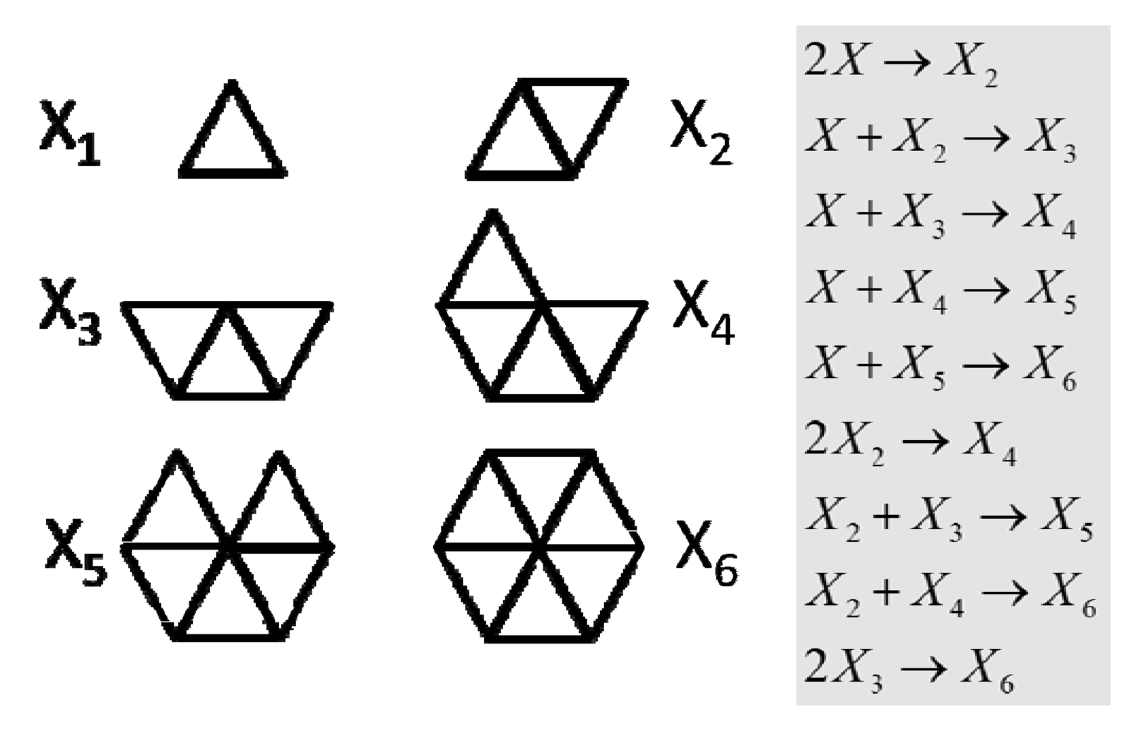
In their 1995 work (The same authors later applied the same model to a simpler self-assembling system, composed of flat sub-millimetric particles that floated at the water-air interface and interacted by capillary flotation forces [87]. The final 4-particle structure and its allowed intermediate products were made predictable by introducing both attractive and repulsive local interactions.), Hosokawa et al. first proposed an explicit analogy with chemical kinetics to model the dynamics of an artificial, macroscopic self-assembling system [28].

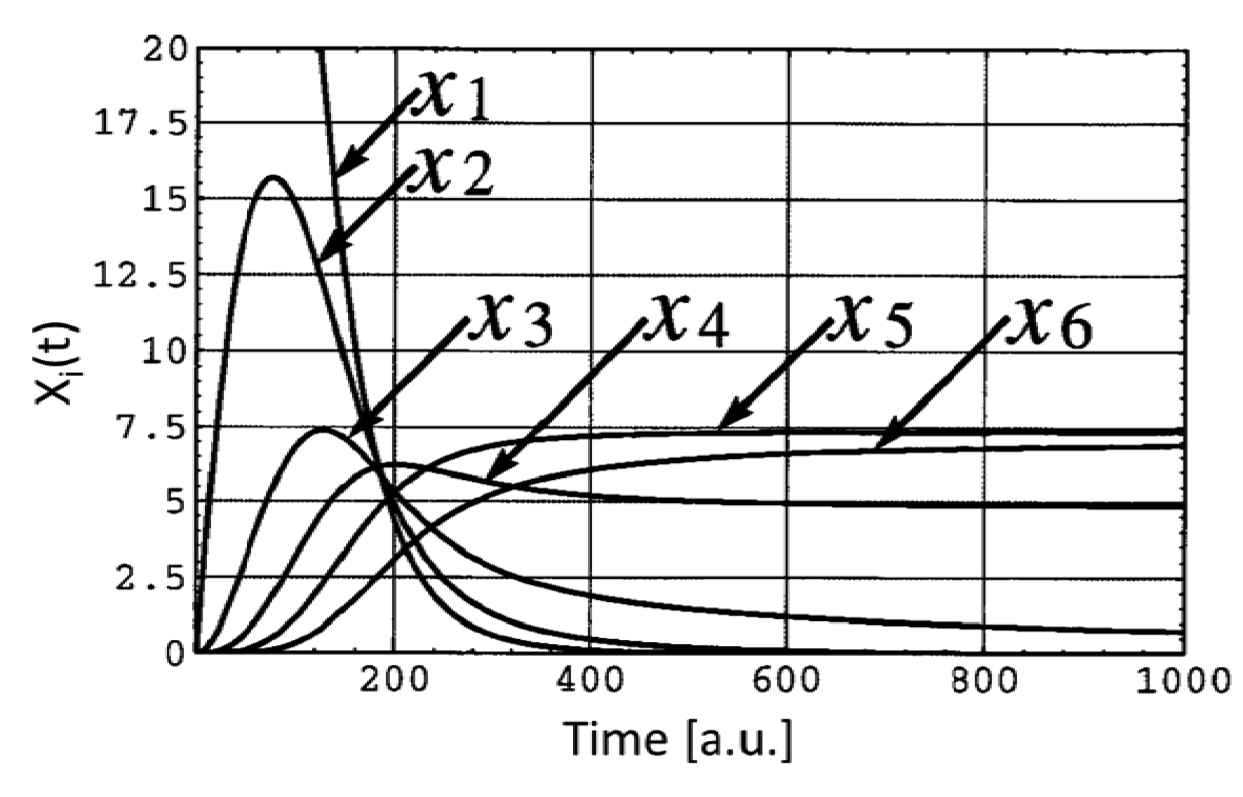
The system was composed of a uniform population of centimeter-sized, polyurethane triangles endowed with neodymium magnets along two of their sides. The flat particles were put in a rotating box which constrained their random motion to a vertical plane. Being equilateral, the assembly of exactly six triangles formed a full hexagon, and all the intermediate assembly products were known a priori (Figure 3). To predict the final population of aggregates after a given assembly time (known as the yield problem), Hosokawa et al. identified the cardinality of the intermediate products of their system with the state variables, and described their evolution from given initial conditions by means of rate and master equations. They considered only bi-particle reactions (Figure 3), and estimated geometrically the particle bonding probability and the rate constants. Their equations predicted that, within a finite time period, not all the initially lone particles would assemble to form complete hexagons, i.e., a few intermediate products would also be part of the final population (Figure 4). They judged their theory was roughly supported by their experiments. In the same work, a conformational switching mechanism was proposed (involving magnets moving across two possible positions) that could make the particles change from non-interactive to interactive. The interactive particles could transfer the property to the assembly products they belonged to. In spite of their expectation, the final assembly yield did not show significant improvement.

3.1.2. Verma's Steady-State Model

In 1995, Verma et al. used the steady-state analysis of rate equations to model the yield of their fluidic SA of silicon particles onto planar substrates templated with binding sites of complementary, three-dimensional shape [88].

Given N_P and n_P representing the total number of particles and that of the unassembled particles, respectively, and N_S, x(t) = x and n_S the total number of binding sites, the filled sites and the vacant sites (with x = N_P − n_P = N_S − n_S), respectively, Verma et al. phenomenologically assumed the assembly rate R_A to be proportional to the number of unfilled sites and to that of the unassembled particles (i.e., R_A ∝ n_Pn_S), and the disassembly rate R_D proportional to the number of filled sites (i.e., self -disassembly, R_D ∝ x). At the steady state (SS), the opposing reaction rates are equivalent, that is:

$${\frac{dx(t)}{dt}|}_{\mathit{\text{SS}}}=0\Rightarrow R_A{|}_{\mathit{\text{SS}}}=R_D{|}_{\mathit{\text{SS}}}$$

(4)

which in this case results in:

$$k_A\cdot n_P{n}_S=k_D\cdot x$$

(5)

where k_A and k_D are rate constants. By defining the filling ratio χ ≡ x/N_S and K ≡ C₁/C₂, Equation 5 yields:

$$\chi =\frac{K·n_P}{1+K·n_p}$$

(6)

which (The analogy of Equation 6 with a first-order superficial adsorption isotherm [89] should not surprise, since assumptions conceptually similar to those of Section 3.1 were also used by, e.g., Langmuir to derive his adsorption isotherm [90]), as intuitively expected, predicts χ → 1 for high values of K and n_P, i.e., for high particle redundancy (n_P » n_S) and for processes favoring stable assembly (K → ∞ for C₂ → 0). Note, however, that Equation 6 is a second-order equation in disguise, since x is not completely resolved.

Recently, Mastrangeli et al. applied the steady-state analysis to predict the yield of more general SA processes, i.e., including multiple disassembly phenomena [3]. Their assembly rate equation was the same as Verma's, while their disassembly rate equation included both self-disassembly and kinetic disassembly, i.e., caused by unassembled particles colliding with assembled ones; that is:

$$R_A=k_A(N_P-x)(N_S-x)$$

(7)

$$R_D=k_{D_1}x+k_{D_2}x(N_P-x)$$

(8)

Solving the SS for x results in (C₁ ≡ k_D1/k_A and C₂ ≡ k_D2/k_A):

$$\chi =\frac{N_S+(1+C_2)N_P+C_1}{2(1+C_2)N_S}-\sqrt{{\left(\frac{N_S+(1+C_1)N_P+C_1}{2(1+C_2)N_S}\right)}^2-\frac{N_P}{(1+C_2)N_S}}$$

(9)

The special cases, including only self-disassembly and kinetic disassembly, can be recovered from Equation 9 by setting C₁ = 0 (Equation 10, analogous to Equation 6) and C₂ = 0 (Equation 11), respectively:

$${\chi }_{\mathit{\text{self}}}=\frac{1}{1+C_2}$$

(10)

$${\chi }_{\mathit{\text{kinetic}}}=\frac{1}{2}+\frac{N_P+C_1}{2N_S}-\sqrt{{\left(\frac{1}{2}+\frac{N_P+C_1}{2N_S}\right)}^2-\frac{N_P}{N_S}}$$

(11)

3.1.3. Zheng and Jacobs' Time-Continuous Model

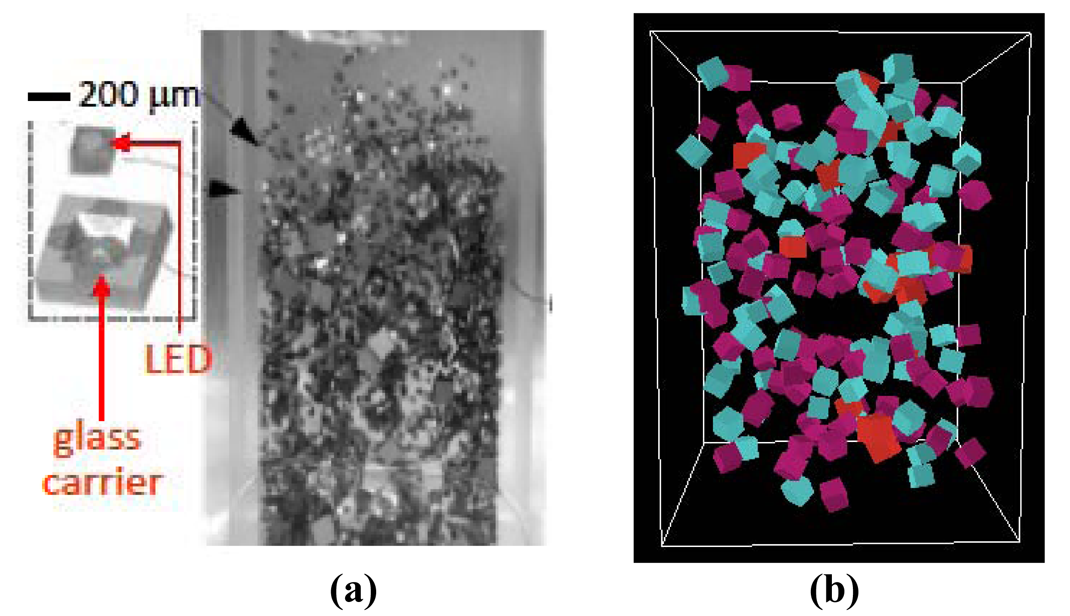
In 2005, Zheng and Jacobs demonstrated a three-dimensional, molten solder-driven and shape matching-directed fluidic process to self-assemble submillimetric LEDs onto glass carriers [91]. In the process, the initial populations of LEDs and carriers are stirred by turbulent flow of warm fluid inside a beaker; by random collisions, the LEDs with sufficient kinetic energy and proper relative orientation fit into the cavities of the carriers, where they are retained by the surface tension of molten solder bumps. To model analytically the yield of their assembly experiments, Zheng and Jacobs proposed a time-continuous rate equation of the following form:

$$\frac{dx(t)}{dt}=\frac{\left[N_C-x(t)\right]\left[N_L-x(t)\right]}{T_A}$$

(12)

where x(t) is the number of assembled dimers, N_C and N_L the total number of carrier and LEDs, respectively, and T_A the single-LED-single-carrier mean assembly time (roughly proportional to the inverse of an assembly rate). Using the initial condition x(t = 0) = 0, Equation 12 is solved by:

$$x(t)=N_C\frac{e^{(N_L-N_C)\frac{t}{T_A}}-1}{e^{(N_L-N_C)\frac{t}{T_A}}-\frac{N_C}{N_L}}$$

(13)

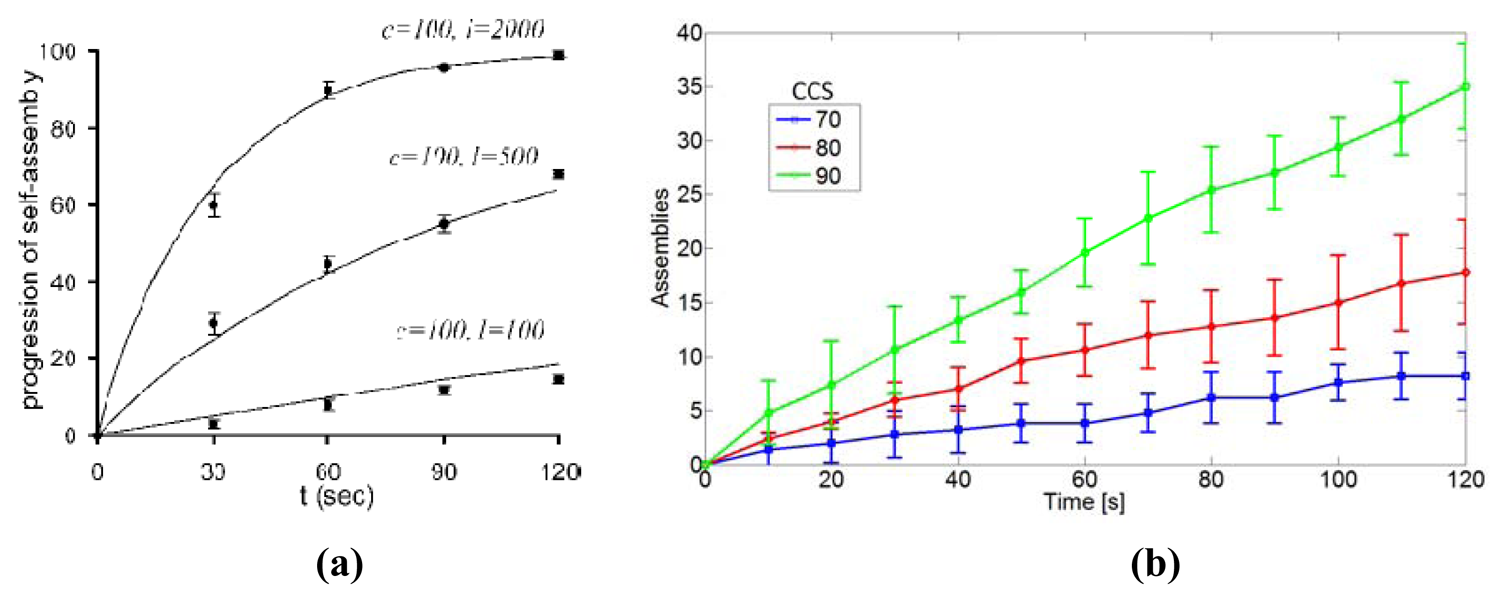
Equation 13 predicts the asymptotic achievement of 100% assembly yield in time by means of stochastic$\text{SA}:\underset{t\to \infty }{lim}x(t)=N_C$. After a given duration of the assembly process, higher assembly yields are predicted for shorter T_A and for larger LED-to-carriers ratios, i.e., particle redundancy. Using T_A as single fitting parameter, the model matched the experimental results accurately (see Figure 7). T_A could be in principle measured experimentally, and depends on design and control parameters.

Mastrangeli et al. [3] generalized Zheng and Jacobs' model by including a generic, second-order (i.e., including mono- and bi-particle events only) disassembly term in Equation 12, obtaining:

$$\frac{dx(t)}{dt}=\frac{\left[N_C-x(t)\right]\left[N_L-x(t)\right]}{T_A}-\frac{D\left[x(t)\right]}{T_D}$$

(14)

where T_D is the single-LED-single-carrier mean disassembly time. Being D[x(t)] of second order in x(t), the solution of Equation 14 has the same form as Equation 13, except for replacing N_L (N_C) with x₁ (x₂), x₁ ≥ x₂ > 0 being the roots of the polynomial in x appearing in the solution of Equation 14 and depending on N_L, N_C, T_A, T_D and the specific coefficients of D[x(t)]. Thus, in this $\text{case}:\underset{t\to \infty }{lim}x(t)=x_2$.

When no disassembly is possible (i.e., T_D → ∞), Equation 12 and consequently Equation 13 are recovered. When kinetic disassembly is considered, i.e., for D[x(t)] = x(t) [N_L − x(t)]/T_D, the roots are: x₁ = N_L and x₂ = N_C /(1 + T_A/T_D). As expected, in this case a finite time-to-disassembly constant implies an asymptotical assembly yield always lower than 100%. D[x(t)] can also take into account further disassembly events specific to three-dimensional SA processes [3].

3.1.4. Critiques to the Models

The rate constants appearing in the previous models lump many interacting factors. Though some of them may be experimentally determined (e.g., mean (dis)assembly time), a complete theoretical model should be able to derive such parameters from first principles describing e.g., the physics of the assembly interactions. On the other hand, such lumping provides a simplification that avoids the models to be application-specific. This, together with the focus on average behavior implicit in the mean-field approach, accounts for the models' high abstraction level.

Multi-particle collision events are not considered. These are less and less probable as the number of parts involved grows (in general, reactions of the form A + B + C → ABC can be decomposed into two bi-reactant reactions A + B → AB and AB + C → ABC without loss of accuracy). Still, they may take place and influence the assembly history. For example, in particle-to-template assembly more than one particle can impinge on the same available binding site, which may constitute a barrier to the filling of its neighboring sites. In three-dimensional SA, the assembled dimers that are then not removed from the assembly space keep on colliding with unassembled parts. Their possible influence is simply neglected in analytical models.

The models predict higher assembly speed and yield for higher particle redundancy. Nevertheless, there could be a practical limit on the maximum number of parts present in a bounded assembly space. Too-high a particle density may increase the chance of damaging collisions, which irreversibly decrease the yield. It may also affect the transport and mixing of the particles themselves, thus altering the assembly rates and making them density-dependent. Therefore, practically speaking, the assumptions listed in Section 3.1 are valid for ensembles containing sparse particles or whose occupied (i.e., excluded) volume is reasonably smaller than the total space volume. These requirements comply with models of ideal solutions and very-diluted gases. In such settings, the discrete nature of assembly events may then not be neglected, i.e., a time-discrete or event-driven framework may be more suitable.

Master equations considering reaction-limited processes—i.e., where diffusion rates are higher than reaction rates—assume ideal stirring and transport mechanisms, as already mentioned. The description of more common and more realistic diffusion-limited aggregation processes [92], where parts can practically have access only to a fraction of the assembly space and thus of particles, requires different mathematical models, possibly involving spatially-dependent diffusion and transport terms [93].

Importantly, all the evoked concepts of particle density, excluded volume and diffusion entail the spatial extent of the particles and of the assembly space. The spatial dimension of (SA) processes is to a large degree eluded in a master equation-based, mean-field analytical approach by conveniently assuming the thermodynamic limit (i.e., an infinite number of point-like particles in an infinite space, such that the particle density is still finite [60]). Spatiality is nonetheless contemplated in lower-level modeling frameworks, such as e.g., the agent-based models presented in the next section.

3.2. Agent-Based Models

Modeling based on the representation of the behavior of system agents is a natural, bottom-up framework to capture the properties of DSs. An agent can be identified with an actual element of the system in object and/or with one of its variables. An Agent-Based Model (ABM) [94] then describes the collective properties of the system that can be inferred and/or emerge from the specification of (i) the agents, (ii) their interaction rules, and (ii) their connection topology [95]. A wide spectrum of topics belonging to disciplines as diverse as sociology [96], economy [97], ecology [95], pattern formation [98], network dynamics, game theory [95,99], videogaming, distributed robotics and many more list ABM as fundamental modeling tool. Recently, ABM was also adopted for the modeling of the SA dynamics of smart particles, as illustrated in the next sections.

3.2.1. Mermoud's Two-Dimensional Model

In 2009, Mermoud et al. proposed an ABM of the stochastic, two-dimensional SA of finite-sized particles within an assembly space with periodic boundary conditions [100]. The particles are circular, and their motion is described by a Langevin stochastic differential equation. Furthermore, the model assumes that the particles invariably aggregate whenever they collide; however, the energy (and stability) of the resulting bond depends on their mutual alignment, as described by the following Arrenhius-like expression:

$$\mathrm{\Delta }E(\xi )=-E_{\mathit{\text{bond}}}\cdot exp\left(-\frac{{\theta }_1^2}{2{\sigma }_{{\theta }_1}^2}-\frac{{\theta }_2^2}{2{\sigma }_{{\theta }_2}^2}\right)$$

(15)

where ξ = (θ₁ θ₂) ∈ [0, π]²is the orientational state vector (i.e., measuring the relative alignment) of the couple of colliding particles, and σ_θ their misalignment tolerance (note that ΔE is negative). The bond energy is used to estimate the assembly (k+) and disassembly (k−) rate constants of the bi-particle aggregate, according to the law of mass action:

$$K=\frac{k_{+}}{k_{-}}=exp\left(-\frac{\mathrm{\Delta }E(\xi )}{E_P}\right)$$

(16)

where E_P is an estimate of the mean energy of the particle systems. Hence, by arbitrarily setting k₊= 1, the value of k₋ derived from Equation 16 is used to estimate the probability of breakup p_b of the bond with energy ΔE(ξ) within the next time interval Δt, according to:

$$p_b\equiv k_{-}·\mathrm{\Delta }t=exp\left(\frac{\mathrm{\Delta }E(\xi )}{E_P}\right)$$

(17)

As a result, the better the alignment, the lower p_b. The model was implemented using NetLogo, an open-source ABM simulation environment developed by Northwestern University [101]. Model results are shown in Figure 10. Interestingly, this model was designed in the context of a more comprehensive, multi-level modeling framework discussed in details in Section 5.

3.2.2. Mastrangeli's Three-Dimensional Model

Mastrangeli et al. [102] proposed in 2010 an ABM of the three-dimensional fluidic SA process earlier demonstrated by Zheng and Jacobs, as a complement to Zheng and Jacobs' own analytical model (see Section 3.1.3).

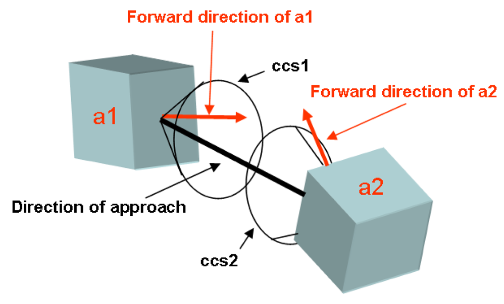
Mastrangeli built a NetLogo model to simulate single realizations of the actual SA process; while simplified, it still elicits important insights into the system dynamics. The assembly space bounded by hard walls closely reproduces the actual one (Figure 5). LEDs and glass carriers are represented by separate species of cuboidal agents with initially equal velocities, random orientations and uniform distribution in the assembly space. They move across space according to Newtonian dynamics without perturbations; particle collisions with walls and with other particles (not leading to assembly, i.e., ineffective) are elastic. The simulation parameters—including particle count, volume, density, initial velocity; space volume, fluidic drag and gravity—can be tuned to reproduce the experimental conditions. Only bi-particle assembly events are considered, producing inert dimers. The assembly events are irreversible (as in the original analytical model), and the particle assembly criterion is geometrical, in strict analogy to the experimental system. Effective assembly events depend on the intersection of the capture cross section (CCS) of two incident particles (Figure 6). Once all parameters are set, the model provides a single fitting parameter (namely, the width θ_CCS of the CCS), in analogy with T_A of Zheng and Jacobs' model. Interestingly, the real-time tracked velocity distribution tends to roughly approach a Maxwell-Boltzmann distribution (as expected for ideal gases, see Section 3.1.4).

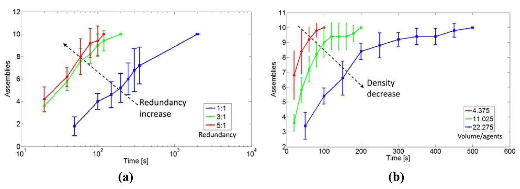
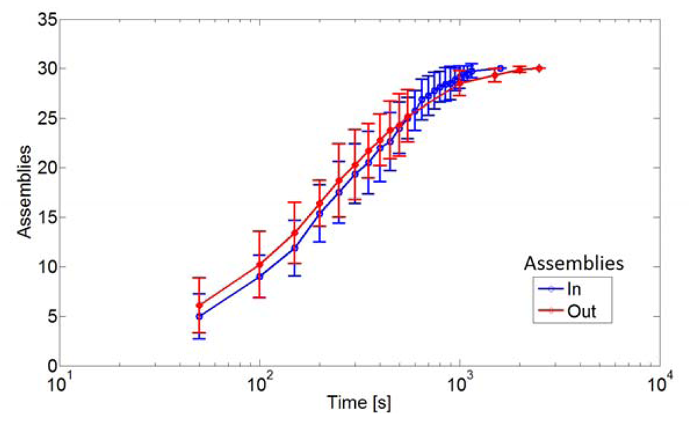
Figure 7compares the ABM and the experimental results for the case N_C = N_L = 100. A good match is found for θ_CCS = 80°, which is then adopted for investigations on other system aspects. For instance, the ABM evidences the influence of the LEDs-to-carriers number ratio [Figure 8(a)], and of the volume of the assembly space (i.e., of the density of the particles, Figure 8(b)) on assembly rates. Moreover, Mastrangeli et al. could investigate the effect of inert dimers on the SA dynamics (Figure 9). As compared to the standard case (labeled in) where the dimers are left in the assembly space after formation, realizations where the dimers annihilate (i.e., are removed from the assembly space) just after formation (i.e., out) show faster (slower) initial (final) assembly dynamics. This preliminary evidence may point out that inert dimers play the role of mechanical assembly catalysts, as additional means of kinetic energy transfer (as also experimentally demonstrated by Baskaran et al. [103]) and/or of compartmentalization of the assembly space. Additional studies are needed to clarify the issue.

3.2.3. Critiques to the Models

Agent-based modeling is particularly suitable to the description of systems involving agents whose behaviors are non-linear (e.g., characterized by non-linear interactions, conditional rules, thresholds), non-Markovian (including memory, path-dependence, hysteresis, adaptation), or of systems in which spatiality and communication play an important role [94]. The agents can also be endowed with arbitrary properties: they can range from fully passive to autonomous. ABM is therefore well consistent with the SMP perspective as it can represent the whole spectrum of distributed systems.

An ABM can produce spatially-embedded simulations of single realizations of the system phenomena. In this sense, agent-based modeling describes physical particle systems at a significantly lower level than e.g., master equations, i.e., with richer, more domain-specific and realistic details, and yet avoiding fully-fledged physical simulations. This can be appreciated by comparing Zheng and Jacobs' (Section 3.1.3) and Mastrangeli's (Section 3.2.2) models of the same fluidic SA process [91], where the latter represents more closely the actual process while not implementing e.g., the physics of molten solder adhesion to metal pads nor hydrodynamic effects (which could nonetheless be accounted for, in principle). Open-source physical engines (e.g., Open Dynamics Engine (Available on: http://www.ode.org/)) or domain-specific soft-wares (e.g., Webots [100]) can be used to produce more physically-accurate simulations.

Additionally, and in spite of its reductionism, an ABM can also capture a system's emergent phenomena, i.e., whose properties (often counter-intuitive) cannot be reduced only to those of its agents [94]. Considering ABM as opposed to analytic, differential equation-based system descriptions is not correct; instead, they are compatible, and even synergetic. This is well illustrated by e.g., Brownian agents (Section 4.2) and, with hindsight, by the remarkable consistency and complementarity of the already mentioned models of Zheng and Jacobs (analytical) and Mastrangeli et al. (ABM), pertaining to the same experimental system. Importantly, one could in principle define a set of coupled dynamical systems that is equivalent to a given ABM. However, the complexity of the resulting system of equations is likely to become intractable; instead, the definition of agents and rules in an ABM is amenable to simple and intuitive approaches, and their sophistication can be tuned and managed with ease—i.e., ABM is more flexible than rate equations. Furthermore, an ABM is more naturally applied when the behavior of agents is better described by interaction rules than by transition rates. Particularly, the stochasticity of the agents' behavior is generally easier to capture in an ABM, especially when one is interested in multimodal, non-parametric, or lumped noise distributions.

Finally, an ABM is essentially a microscopic modeling approach. Therefore, its primary alternative is a macroscopic modeling approach, of which master equations (Section 3.1) or other mean-field approaches are specific, but not exclusive, instances. A relaxation of this duality suggests using a hierarchy of models to describe the same system at different levels of abstraction (concerning details, information, length and time scales and their continuity versus discreteness). We note that several levels of description can coexist within the same ABM, especially when the introduction of agent subgroups or aggregates is meaningful or legitimate within a system (see Section 4.2). A different and possibly more general approach to multilevel modeling, featuring models belonging to different frameworks, is presented in Section 5.

4. Modeling the SA Dynamics of Active Particles

The following sections illustrate models that can be partly considered extensions of those discussed in Section 3, as they can also capture programmed particle actions (e.g., planned structure formation) and thus span wider fields.

4.1. Stochastic Reaction Models

Originating from chemistry, stochastic reaction models are ways to macroscopically represent continuous-time Markov processes.

To specify a Markov process X(t), the transition rate matrix from state j to state i (or generator) A_ij can be given, such that:

$$p\left\{X_i(t+dt)|X_j(t)\right\}=A_{ij}dt$$

(18)

And the probability distribution at time t given an initial distribution p₀ is given by:

$$p\left\{X_i(t)\right\}={\left(p_0\cdot e^{tA}\right)}_i$$

(19)

In some cases, A is too large to be easily tractable; but the structure of the process may be used to simplify its description. A stochastic reaction model then assumes a finite set of system states at time t, X⃗(t) = [X₁ (t)…X_s (t)…X_S(t)] with X_s(t) representing the number of elements in species s. Each change in species populations is associated with a reaction r producing effect e⃗_r, such that x⃗ → x⃗ + e⃗_r takes place in the next time interval dt at a rate given by the propensity function h_r (x⃗). Without significant loss, A can accordingly be described by:

$$A(\overrightarrow{x},\overrightarrow{x}+{\overrightarrow{e}}_r)=h_r(\overrightarrow{x})$$

(20)

$$\begin{array}{ccc}A(\overrightarrow{x},\overrightarrow{x}\prime )=0& if\overrightarrow{x}+{\overrightarrow{e}}_r\ne \overrightarrow{x}\prime & \forall r\end{array}$$

(21)

$$A(\overrightarrow{x},\overrightarrow{x})=-\sum _r{h}_r(\overrightarrow{x})$$

(22)

A stochastic reaction network is a stochastic reaction model with S species and R reactions. Each reaction has the form:

$$a_1{X}_1+a_2{X}_2+\dots \stackrel{{\lambda }_r}{\to }{b}_1{Y}_1+b_2{Y}_2+\dots$$

(23)

where X_i (Y_i) are the number of elements in the reactant (product) species i, λ_r is the reaction rate constant, and a_i and b_i are stoichiometric coefficients such that the reaction effect is in their difference.

Hosokawa's idea of identifying intermediate assembly products with state variables (see Section 3.1.1) can be partly inscribed in the framework of stochastic reaction networks. Explicitly inspired by Hosokawa's work, Klavins et al. proposed a grammatical graph-based variant [104]. They identified the intermediate assembly products with the labeled nodes of a graph, whose labeled links describe general rules (representing physical interactions or the possibility of active choices made by the agents) given to derive the hierarchy of possible products accessible from a given initial condition. Such graph grammars can be translated into a set of hardware specifications; they were used by Klavins' group to model the collective behavior of aggregating reflexive robots. Their programmable parts resemble Hosokawa's triangular magnetic particles; they move randomly on an air table, are able to communicate and share their internal states upon contact, and eventually assemble by means of magnetomechanic latches [53]. Recently, they demonstrated a feedback controller for the copy number of assemblies described by a tunable reaction network [105]. The Tribolon system proposed by Miyashita et al. can be considered as a simpler self-assembling system as compared to Klavins'; among other objectives, it was used for modeling the impact of particle morphology on the yield of two-dimensional SA [68].

A single realization of a reaction process reduces to tracing a sample path through the system's set of states starting from specific initial conditions. Gillespie derived an exact numerical algorithm for the simulation of stochastic processes [106]. Gillespie's direct method is based on the following property of the chemical reaction models. Let T⁺ be the time at which the next reaction occurs, as counted from instant t; then, given X⃗(t) = x⃗₀:

• the conditional distribution of T⁺ −t is exponential with parameter μ = Σ_rh_r (x⃗₀);

• the conditional probability p(R = r₀) for the next reaction to be r₀ is $\frac{h_{r_0}({\overrightarrow{x}}_0)}{{\Sigma }_r{h}_r({\overrightarrow{x}}_0)};$

• T⁺ −t and the choice of r₀ are conditionally independent.

The algorithm can then be described as follows: starting from the initial condition x⃗₀ at time t = 0, at each step: draw T⁺ from the exp(μ) distribution, and set t → t + T⁺; if t < t_max, then draw R from p(R = r₀), and set X⃗ → X⃗ + e⃗_r.

Gillespie developed several computationally more efficient variants of the original numerical algorithm, as well [60]. Moreover, he showed that the default rules for the propensity functions are valid for well-stirred chemical reactions (Section 3.1); nevertheless, they are also generally accepted for many bio-chemical and population models. Napp et al. proposed an extended state space approach based on hidden Markov models—i.e., models where the system is assumed to be Markovian but with unobserved states—to deal with stochastic SA of non-well stirred ensembles of particles [107]. Stochastic simulations with spatial resolution were also developed. Smoluchowski models can account for spatial diffusion phenomena as applied, e.g., to chemical reactions with molecular detail [93]; the Fokker-Plank diffusion model was also adopted by Prorok et al. to capture the spatial distribution over time of miniature robots in an inspection task [108].

4.2. Brownian Agents and Stochastic Micro-Agents

With his Brownian agents, Schweitzer introduced a rather comprehensive modeling framework for DSs, both agent-based and supported by the analytical methods of statistical mechanics [109].

Each agent k is described by a finite set of state variables $\left\{u_i^{(k)}\right\}$, whose dynamics are subject to a superposition of both deterministic (f ^(k)) and stochastic (f^stoch) influences, as captured by the Langevin formalism:

$$\frac{d{u}_i^{(k)}}{dt}=f_i^{(k)}+f_i^{\mathit{\text{stoch}}}$$

(24)

where the distinction between the two types of causes depends on whether they can be possibly resolved at the characteristic time and length scales of the chosen agents—in analogy with physical particles undergoing Brownian motion; hence the name of such agents. f ^(k) subsumes all specifiable influences on the state variables, such as non-linear, rule-based interactions with other agents, external conditions as defined by control parameters (e.g., dissipative forces, forces deriving from external potentials, in/outflux of resources), and internal time-dependent agent dynamics. On the other hand, f^stoch cumulates all influencing factors that would require a smaller-scale observation to be detailed into a single stochastic variable with defined statistical properties. The scale at which such distinction is placed sets the degree of granularity in the description of the system. This possibility of choosing the level of detail abstraction is useful to distill meaningful collective information, and to allow the subsequent, cumulative buildup of model complexity to remain tractable.

The Brownian agent approach is focused on cooperative agent interactions, particularly self-organization and aggregation, instead of on individual actions. Brownian agents are not able of deliberative actions, e.g., calculating cost functions and develop internal world representations and strategies. Still, they possess internal degrees of freedom, for instance an internal energy depot; and they can interact indirectly by means of stigmergy [6], i.e., by modifying the shared environment that in turn influences the actions of the (other) agents.

Upon the baseline of purely passive agents undergoing Brownian motion, Schweitzer adopts a minimalistic, constructive agent design, in which the complexity and potentialities of each agent are progressively augmented by the cumulative addiction of built-in features and capabilities. For each subsequent level of agent sophistication, the simplest set of rules is used and a homogeneous population of agents is simulated to investigate its collective properties and potential behavior(s). This way, Schweitzer shows that Brownian agents can be progressively enabled to perform or reproduce various collective patterns, e.g., deterministic chaotic, intermittent or swarming type of motion; simulations of aggregation and structure formation processes of physico-chemical systems; self-organization of stable and adaptive networks; trail formation, and consequent reinforced biased random walk; and social aggregation phenomena, like urban sprawl and opinion formation, as well [109]. Other researchers also adopted Brownian agents for e.g., traffic modeling, synchronization phenomena, granular matter, and more.

As an interesting alternative, Milutinović proposed a framework linking directly the microscopic, deterministic behavior of agents to the macroscopic dynamics of their populations, as inspired by the kinetic gas theory [110]. His stochastic micro-agents are hybrid automata described by event-driven transitions among a discrete set of control states and by time-dependent motion in a continuous space. The events reproducing inter-agent interactions and inducing the control state transitions are generated by a collection of event generators; these events are stochastic, and their probability distributions encode the complexity of the interactions within a population of agents. That is, a mean-field approach is adopted, where each agent interacts with the rest of the agents in the population through their aggregate effects, as embodied in the event sequences produced by the event generators. Importantly, a set of partial differential equations (shown to be a generalization of the Liouville equation) describes the time evolution of the probability density function associated with the agent population given its initial conditions. This way, collective dynamics can be directly derived from that of the individual agents. The framework was originally applied to the modeling of immune system cells.

4.3. Critiques to the Model

Stochastic reaction networks' abstraction level lies between that of mean-field differential equations and of agent behavior-oriented ABMs. Particularly, they are not as spatially embedded as the latter; yet, in contrast to more abstract mean-field models, they can include network topologies. In fact, their strength resides in taking advantage of the developing tools of network theory [111] to quantitatively describe the local geometrical neighborhoods of agents and the informational aspects of their interactions. For instance, at the core of important results in burgeoning fields, e.g., biological networks for the regulation of genetic expression, metabolisms and catalytic reactions lies the network analysis by combined use of rate equations and logical operators [112]. Klavins' graph grammars are an actual example of how similar methods can be applied to SMPs [53]. On the other hand, the Markovian assumption underlying the stochastic reaction models may constrain their application to systems of shallower complexity, as compared to those addressable by ABMs.

Brownian agents provide an important example of a reductionist but nevertheless constructive approach to describe a wide range of DSs at several scales and increasing levels of sophistication and complexity—in a way reminding of Braitenberg's cumulative design of vehicles [113]. By combining analytic and agent-based representations at nearly all levels, Schweitzer's approach can exploit their complementary features (e.g., statistical mechanics tools and flexible design, respectively) and tune their relative weight in the aggregated models according to case-specific applications. Reaching from passive, purely reactive agents to active, fully reflexive ones, Brownian agents represent therefore a modeling tool remarkably well aligned with SMPs, since the latter shall, in principle, span the entire domain of the former (as outlined in Section 1). However, the flexibility of such agents is traded off for a limited anchoring to reality—that is, the agents are rather abstract and defined by parameters not derived, at least explicitly, from an underlying, submicroscopic level of detail (see next section for a definition). Importantly, from Schweitzer's work it is not straightforward to derive univocal design guidelines to embed his software agents into real devices, nor are many of the parameters governing the agents' behavior directly traceable back to experimental details and features. An extension oriented toward model-based design and bridging the model/reality gap is therefore required for the present framework to fully fit within our SMP perspective.

In Milutinović's framework, the collective macroscopic dynamics is directly connected to the microscopic agent dynamics through the evolution of the associated probability distribution, while the actual interactions among agents are lumped, and their complexity hidden, into the stochastic components of the event generators. It represents an interesting attempt at including both macroscopic (mean-field) and microscopic (individual agent) modeling levels within the context of hybrid automata control; it is also amenable to analytical treatment, especially in the Markovian approximation.

Finally, stochastic reaction networks and hybrid automata can also be readily included into an even more comprehensive modeling framework—i.e., one integrating a hierarchy of different modeling tools or methods, each specific and/or more suitable to a particular level of abstraction, within a single and consistent modeling suite. This refers to the general multi-level modeling framework, in which the choice of the model types itself, beside necessarily their instances, can be case-specific. In the next section, we illustrate the multi-level modeling approach as applied to the self-assembly of SMPs.

5. Toward a Comprehensive Modeling Framework for SMPs: Multi-Level Modeling

One of the main difficulties in modeling ensembles of SMPs, and particularly those involving aggregation and self-assembly, is the inherent randomness and hybridness of their dynamics. For instance, while a robot's controller is essentially a deterministic, discrete entity, it has to interact with a noisy, continuous environment. At the microscale, a particle's binding site may or may not be occupied (discrete state variable), and this may depend on the temperature of the system (continuous parameter), such as in the case of e.g., DNA-mediated binding sites.

These challenges motivate the combination of multiple levels of abstractions—ranging from detailed, submicroscopic models up to more general, macroscopic ones—into a consistent multi-level modeling framework. On the one hand, one needs submicroscopic models that are able to capture the complete state of particles, including spatiality and embodiment (e.g., pose, shape, surface properties). On the other hand, one is also interested in models that can yield accurate numerical predictions of collective metrics, and investigate, possibly in closed form, macroscopic properties such as the sizes, types, and proportions of the resulting assemblies. Multi-level modeling allows the fulfillment of both requirements in a very efficient way by building up models of increasing levels of abstraction in order to capture the relevant features of the system.

Within this context, we classify models of distributed systems into three main categories: (i) submicroscopic models, in which each particle's state as well as sub-components (e.g., bulk, surfaces, binding sites) are captured (Section 5.1); (ii) microscopic models, in which the state of each particle in the system is captured, but the details of its sub-components are abstracted (Section 5.2), and (iii) macroscopic models, in which all particles in a given state are aggregated into a single state variable (Section 5.3).

Originally, the multi-level modeling methodology was developed in the context of swarm robotics [114]; in [100], Mermoud et al. extended this approach to more minimalist entities, prefiguring the more mature concept of SMPs. In the sequel, we describe a suite of models at different abstraction levels, all exemplifying higher abstractions of Mermoud's two-dimensional ABM described in Section 3.2.1.

5.1. Submicroscopic Models

The most detailed level of modeling is provided by physics-based simulations, which bridge the gap between model and reality by accurately capturing each system particle as well as its sub-components. These simulations faithfully account for a subset of physical phenomena (e.g., capillarity, hydrophobic interaction, electromagnetic forces), which are considered most relevant to the dynamics of the system. The strength of this type of models is their direct anchoring to reality, even though the number of their parameters tends to grow rapidly with the number of physical phenomena to be modeled. Also, while these models enable, in principle, the direct visualization of a particle's behavior, their heavy computational requirements limit their applicability to systems that involve a limited number of particles. Examples include finite-element numerical simulations and molecular dynamics (representing the most radical physical ABM) for M/NEMS (see Section 2.3), and case-specific software faithfully reproducing robot behaviors, such as Webots [115].

5.2. Microscopic Models

Even though microscopic models capture the state of each individual particle in the system, their state vector is significantly smaller than their correspondingly submicroscopic counterpart. This state reduction is typically obtained through appropriate aggregation of the state variables, which can be more or less important as a function of the desired level of detail. Section 3.2 described two such, spatial models. Spatial models offer an interesting modeling framework for multi-agent systems, but they can be expensive both in terms of memory and computation. Indeed, these models store the position and the orientation of each agent as well as the precise structure of each aggregate. Also, they must determine whether a collision occurred, or not, at each iteration and for each pair of agents.

One can go even further in the process of abstracting details that are not significant to the dynamics of the process under investigation. Hereafter we describe a Monte Carlo-based version of the ABM presented in Section 3.2.1 which does not capture spatiality, i.e., it does not keep track of the position and orientation of each agent. It can be considered a stochastic microscopic model that, in contrast to the macroscopic models developed later, does not rely on a mean-field approach in terms of population distribution. However, the model assumes that the individual behavior of each agent and that of the environment can be represented by (semi-)Markov chains, i.e., the probabilistic transition from one state vector A to another state vector B depends only on the information contained in the state vector A (see Section 3.1).

A Non-Spatial Monte Carlo Model

This model assumes that agents aggregate pair-wise to form dimers only, and it keeps track of only one property of the dimers, that is, the relative alignment of their building blocks. Since the model is non-spatial, collisions are no longer deterministic, but are instead randomly sampled from a Poisson distribution of mean λ = p_cN_s (see Equation 25). Furthermore, each aggregate resulting from agent collisions is individually captured: a random relative alignment ξ_i = (θ_1,i θ_2,i) is generated and stored in a list Ξ_a (see Algorithm 1). One interesting feature of this type of models is that they store only relevant pieces of information about the aggregates, which can range from the number of building blocks to a fully-fledged graph-based representation of the aggregate's topology.

One subtlety in building non-spatial models of aggregation is to accurately capture the encountering probabilities. Here, we assume a constant encountering probability p_c that is determined using a geometric approximation:

$$p_c\approx \frac{\widehat{v}T{w}_d}{A_{\mathit{\text{tot}}}}$$

(25)

v̂ is the average velocity of the particle, w_d its diameter, T the sampling time, and A_tot is the total area of the arena [114]. In more complicated scenarios, one would also account for encountering probabilities that depend on the size and the geometry of the aggregates.

Algorithm 1. Pseudo-code of the non-spatial Monte Carlo simulation.

Initialize Ns = N0 and N2,3,… = 0

for all t in tspan do

– Sample nc the number of collision events from a Poisson distribution of mean λ = pjoinNs – Generate and append to Ξa a random vector of nc relative alignments Ξc = (ξ1, …, ξnc) with ξi = (θ1,i, θ2,i)and θd,i ∼ u(0, π) – Generate a random vector $x_i^s~u(0,1)$ with and Na = size(Ξa) – Compute nb the number of aggregates in Ξa with ξi such that $x_i^s$ < pleave (ξi) and remove them from Ξa – Let N ← N + 2 nb − 2 nc

end for

5.3. Macroscopic Models

The stochastic model previously described provides a single realization of the time evolution of the system at each run, and do not scale well with the number of robots. As a result, one must usually perform a large number of computationally expensive runs in order to obtain statistically meaningful results. Hereafter, we describe a non-spatial macroscopic version of the previous model of aggregation, which allows one to overcome these limitations, but at the price of further approximations.

Macroscopic models can also track properties of the aggregates other than their size (i.e., the number of building blocks), such as their geometry. To achieve that, one conventional approach is to discretize selected state variables into several sub-variables, essentially going through a state expansion process. For instance, in order to capture the alignment of pairs of building blocks, one can discretize the state variable N₂ (representing the average number of dimers) into M sub-variables N_2,i that denote the number of aggregates with an average alignment ξ_i with i = 1,…,M. Obviously, such a discretization leads to a M-fold increase of the number of states, and therefore an exponential increase of the number of equations, making the model rapidly intractable. The proposed macroscopic model captures alignment of building blocks at the macroscopic level by using this approach, but with an explicit limitation on the size of the aggregates to pairs.

A Macroscopic Model of Pair-wise SA

One can describe the dynamics of each particle P by a Markov chain with a set of states X. The state space X^(P) should be discrete, finite, and it must reflect the type of the aggregate s the particle belongs to. However, the space S of aggregate's types in our model is not discrete. Indeed, even though we can distinguish between single building blocks and pairs in a discrete manner, pairs take continuous energy values (see Section 3.2.1). To discretize S, we note that the symmetry of Equation 16 allows simplifying the vector ξ defining the relative particle orientation within an aggregate to a scalar, i.e., the norm of the relative positioning, denoted by:

$${\theta }^2=\Vert {\xi }^2\Vert ={\theta }_1^2+{\theta }_2^2\in \left[02{\pi }^2\right]$$

(26)

which can be discretized into a set of K averaged values θ̂₁² given by:

$$\begin{array}{ccc}{\widehat{\theta }}_1^2=\left(i-\frac{1}{2}\right)\cdot \frac{2{\pi }^2}{K}& \mathit{\text{with}}& i=1,2,\dots K\end{array}$$

(27)

Therefore, the state space of the Markov chain is given by:

$${\text{X}}^{(P)}=s_i\in S_d$$

(28)

With S_d the discretized space of aggregate's types, s₀ representing single particles, s_i pairs with an averaged relative positioning norm θ̂₁² with i = 1,2…K and binding energy

$$\mathrm{\Delta }E(s_i)=E_{\mathit{\text{bond}}}\cdot exp\left(\frac{{\widehat{\theta }}_1^2}{2{\sigma }_{\theta }^2}\right)$$

(29)

Therefore, the probability for a particle P to aggregate with another particle into a pair of averaged relative positioning norm θ̂₁² is:

$$p({\text{X}}^{(P)}(t+1)=s_i|X^{(P)}(t)=s_0)=1$$

(30)

Similarly, the probability for a particle P to leave a pair with an averaged relative positioning θ̂₁² is given by:

$$p({\text{X}}^{(P)}(t+1)=s_0|X^{(P)}(t)=s_i):S_d\to [01]$$

(31)

and will be denoted p_l(s_i). A pair will break up if one or both of its particles leaves. Therefore, the probability p_b(s_i) for a pair of type s_i to break up (Equation 17) can be written as:

$$\begin{array}{c}{p}_b(s_i)=1-{\left[1-p_l(s_i)\right]}^2\\ =p_l(s_i)\cdot \left[2-p_l(s_i)\right]\\ =exp\left(\frac{\mathrm{\Delta }E(s_i)}{\alpha v_s^2}\right)\end{array}$$

(32)

Using a set of difference equations, one can summarize the average state transitions of each individual Markov dynamical system, and thus keep track of the number of aggregates of type s ∈ S_d. We write N_i the average number of aggregate of type s_i.

The average number of single particles N_s is given by the following difference equation:

$$N_s(t+1)-N_s(t)=2\langle {\overrightarrow{p}}_b{\overrightarrow{N}}_p(t)\rangle -p_c\cdot N_s{(t)}^2$$

(33)

having defined

$${\overrightarrow{p}}_b={\left[p_b(s_1),\dots ,p_b(s_K)\right]}^T$$

(33)

$${\overrightarrow{N}}_p(t)={\left[N_1(t),\dots ,N_K(t)\right]}^T$$

(33)

and p_c is the collision probability (Equation 25) and 〈..〉 is the scalar product. The scalar term 〈p⃗_bN⃗_b (t)〉 is the average number of pairs that broke up at iteration t. The term p_c·N_s(t)² is the average number of particles that collided and formed a pair at iteration t. Similarly, the number of pairs of type s_i with i = 1,…,K is given by the following difference equation:

$$N_i(t+1)-N_i(t)=f(i)\cdot \frac{p_c\cdot N_s{(t)}^2}{2}-p_b(s_i)\cdot N_i(t)$$

(34)

where f (i) : Z₊ → [0, 1]. The term p_b (s_i) · N_i (t) is the average number of pairs of type s_i that broke up at iteration t. The term p_c · N_s(t)² is the average number of particles that collided and formed a pair at iteration t, regardless of its type (since two particles are needed to form a pair, this term is divided by two). Furthermore, since all formed pairs are not of type s_i, the function f (i) determines the fraction of formed aggregates that are actually of type s_i (refer to [100] for a complete derivation of f (i)).

5.4. Validation of and Critiques to the Models

Mean-field macroscopic models can be computationally efficient; but they are approximations of the models at lower abstraction levels and, ultimately, of the real system. Particularly, mean-field macroscopic models aggregate discrete entities into real-valued state variables that describe averaged quantities. This way, both the absolute discrete quantities of the state variables representing the number of agents in a given state and the potentially non-uniform behavior of the system under consideration are lost. To cope with it, macroscopic models rely on the ODE approximation, which assumes that the system involves a large number of small changes, i.e., the model becomes exact if the system is scaled such that the reaction rates become large and the effects of those reactions small (i.e., in the thermodynamic limit, Section 3.1.4). The validity of the approximation does not only depend on the number of particles in the systems, though: the number of interactions and the structure of their network also play a key role. Hence, discretization of state variables is generally a source of inaccuracy, because it tends to lower the reaction rates while increasing their effects.

Figure 10 provides a comparison of the predictions of the models of the same system presented in Sections 3.2.1 (microscopic, spatial), 5.2.1 (microscopic, non-spatial) and 5.3 (macroscopic), respectively. For N₀ = 1,000, all models show a good agreement, even though the Monte Carlo and the macroscopic model exhibit a slightly faster convergence, probably due to their non-spatiality. Indeed, a particle that is surrounded by stable aggregates may take quite some time before encountering another single particle. Such suboptimal mixing tends to slow the process down; this phenomenon is not captured by non-spatial models, but has been repeatedly reported in spatial ABMs (Section 3.2).

Also, one can clearly see that the accuracy of the macroscopic model with respect to the Monte Carlo one degrades gracefully as N₀ decreases; for N₀ = 50, the macroscopic model actually predicts a much faster growth of the pair ratio than that observed in Monte Carlo simulations, whereas an almost perfect match is observed for N₀ = 500. These results exhibit the limits of the ODE approximation for nonlinear dynamical systems. More complex behaviors are observed when varying the discretization factor K (full details in [100]).

6. Conclusions and Perspectives

This paper proposed a novel and unifying perspective for the design and control of self-assembling micro-/nano- and distributed intelligent systems. This perspective results from the extrapolation of ongoing technological trends observed in these domains, namely smarting and minimalism, respectively. We believe that, thanks to such trends, both domains will converge and eventually merge into a single locus, defined by what we call smart minimal particles (SMPs). SMPs bridge the complexity and scale gap between micro/nanosystems and robotic systems; contextually, SMPs point to the existence of a continuum of sophistication between passive and active particles, both from a technological and a methodological standpoint. Moreover, the proposed unification emphasizes the cross-fertilizations among the originally separate domains concerning terminologies and methodologies. Particularly (but not exclusively) in the case of the modeling of aggregation and self-assembly dynamics, the mutual advantages of shared knowledge and tools are evident and very promising, as we showed in reviewing the efforts pursued in both M/NEMS and distributed robotics in terms of manufacturing technology and distributed control strategies.

A major motivation for proposing the concept of SMPs is the development of the vast, necessarily multi-disciplinary knowledge required to master the control of the hierarchical organization of matter into adaptive artificial structures—i.e., programmable matter (see e.g., [116-118] for related acceptions). In this context, we consider M/NEMS as an enabling technology, which shall ultimately allow for the organization of matter from its raw state into small yet functional particles, smart enough to achieve further aggregation into larger and more sophisticated entities; at the same time, distributed robotics is elaborating and developing control strategies for the decentralized and robust coordination of such building blocks into the desired, adaptive structures. Therefore, in our view, the introduction of SMPs is a natural step towards a seamless, bidirectional flow of information and capabilities all the way from the most basic micromachined particles to fully-fledged robots.

This paper accordingly attempted to put the collective efforts of vast research communities into a shared perspective—as a step toward the ambitious direction outlined above. We are actively pursuing both technological and theoretical investigations on SMPs, and it is our hope that the introduction of the SMP perspective may help favoring stronger and fruitful interactions among the M/NEMS and robotics communities so to catalyze further research into self-assembly—needed to pursue the targeted goals and to cope with the many challenges yet to be tackled by both communities.

References

- Caramazine, S.; Deneubourg, J.-L.; Franks, N.R.; Sneyd, J.; Theraulaz, G.; Bonabeau, E. Self-Organization in Biological Systems; Princeton University Press: Princeton, NJ, USA, 2001. [Google Scholar]
- Warneke, B.; Last, M.; Liebowitz, B.; Pister, K.S.J. Smart dust: Communicating with a cubic-millimeter computer. IEEE Comput. 2001, 34, 44–51. [Google Scholar]
- Mastrangeli, M.; Abbasi, S.; Varel, C.; Van Hoof, C.; Celis, J.-P.; Böhringer, K.F. Self-Assembly from milli- to nanoscales: Methods and applications. J. Micromech. Microeng. 2009, 19, 083001. [Google Scholar]
- Floreano, D.; Mattiussi, C. Bio-Inspired Artificial Intelligence; MIT Press: Cambridge, MA, USA, 2008. [Google Scholar]
- Tolley, M.; Kalontarov, M.; Neubert, J.; Erickson, D.; Lipson, H. Stochastic modular robotics systems: a study of fluidic assembly strategies. IEEE Trans. Robot. 2010, 26, 518–530. [Google Scholar]
- Theraulaz, G. A brief history of stigmergy. Artificial Life 1999, 5, 97–116. [Google Scholar]
- Holland, O.E.; Melhuish, C. Stigmergy, self-organization and sorting in collective robotics. Artificial Life 1999, 5, 173–202. [Google Scholar]
- Hsieh, M.A.; Kumar, V.; Chaimowicz, L. Decentralized controllers for shape generation with robotic swarms. Robotica 2008, 26, 691–701. [Google Scholar]
- Böhringer, K.; Brown, R.; Donald, B.; Jennings, J.; Rus, D. Distributed robotic manipulation: Experiments in minimalism. In Experimental Robotics; Khatib, O., Kenneth Salisbury, J., Eds.; Springer: Berlin, Germany, 1997; Volume IV, pp. 11–25. [Google Scholar]
- Madou, M.J. Fundamentals of Microfabrication and Nanotechnology, 3rd ed.; CRC Press: Boca Raton, FL, USA, 2010. [Google Scholar]
- Morris, C.J.; Stauth, S.A.; Parviz, B.A. Self-assembly for microscale and nanoscale packaging: Steps toward self-packaging. IEEE Trans. Adv. Pack. 2005, 28, 600–611. [Google Scholar]
- Frutiger, D.R.; Vollmers, K.; Kratochvil, B.E.; Nelson, B.J. Small, fast, and under control: Wireless resonant magnetic micro-agents. Int. J. Robot. Res. 2010, 29, 613–636. [Google Scholar]
- Rechtsman, M.; Stillinger, F.; Torquato, S. Designed interaction potentials via inverse methods for self-assembly. Phys. Rev. E 2006, 73, 011406. [Google Scholar]
- Böhringer, K.F.; Donald, B.R.; MacDonald, N.C. Programmable vector fields for distributed manipulation, with applications to MEMS actuator arrays and vibratory parts feeders. Int. J. Robot. Res. 1999, 18, 168–200. [Google Scholar]
- Donald, B.R.; Levey, C.G.; Paprotny, I. Planar microassembly by parallel actuation of MEMS microrobots. IEEE J. Microelectromech. Syst. 2008, 17, 789–808. [Google Scholar]
- Knuesel, R.J.; Jacobs, H.O. Self-assembly of microscopic chiplets at a liquid-liquid-solid interface forming a flexible segmented monocrystalline solar cell. Proc. Nat. Accad. Sci. USA 2010, 107, 993–998. [Google Scholar]
- Stauth, S.A.; Parviz, B.A. Self-assembled single-crystal silicon circuits on plastic. Proc. Nat. Accad. Sci. USA 2006, 103, 13922–13927. [Google Scholar]
- Zheng, W.; Chung, J.; Jacobs, H.O. Fluidic heterogeneous microsystem assembly and packaging. IEEE J. Microelectromech. Syst. 2006, 15, 864. [Google Scholar]
- Morris, C.J.; Ho, H.; Parviz, B.A. Liquid polymer deposition on free-standing microfabricated parts for self-assembly. IEEE J. Microelectromech. Syst. 2006, 15, 1795–1804. [Google Scholar]
- Mastrangeli, M.; Ruythooren, W.; Van Hoof, C.; Celis, J.-P. Conformal dip-coating of patterned surfaces for capillary die-to-substrate self-assembly. J. Micromech. Microeng. 2009, 19, 045015. [Google Scholar]
- Saeedi, E.; Abbasi, S.; Böhringer, K.F.; Parviz, B.A. Molten-alloy driven self-assembly for nano and micro scale system integration. Fluid Dyn. Mater. Process. 2007, 2, 221–246. [Google Scholar]
- Shetye, S.B.; Eskinazi, I.; Arnold, D.P. Magnetic self-assembly of millimeter-scale components with angular orientation. IEEE J. Microelectromech. Syst. 2010, 19, 599. [Google Scholar]
- Onoe, H.; Matsumoto, K.; Shimoyama, I. Three-dimensional sequential self-assembly of microscale objects. Small 2007, 3, 1383–1389. [Google Scholar]
- Lee, S.W.; Bashir, R. Dielectrophoresis and chemically mediated directed self-assembly of micrometer-scale three-terminal metal oxide semiconductor field-effect transistors. Adv. Mat. 2005, 17, 2671–2677. [Google Scholar]
- Tanemura, T.; Lopez, G.; Sato, R.; Sugano, K.; Tsuchiya, T.; Tabata, O.; Fujita, M.; Maeda, M. Sequential and selective self-assembly of micro components by dna grafted polymer. Proceedings of IEEE 22nd International Conference on Micro Electro Mechanical Systems (MEMS09), Sorrento, Italy, 25–29 January 2009.
- Barish, R.D.; Schulman, R.; Rothemund, P.W.K.; Winfree, E. An information-bearing seed for nucleating algorithmic self-assembly. Proc. Nat. Accad. Sci. USA 2009, 106, 6054–6059. [Google Scholar]
- Saitou, K. Conformational switching in self-assembling mechanical systems. IEEE Trans. Robot. Autom. 1999, 15, 510–520. [Google Scholar]
- Hosokawa, K.; Shimoyama, I.; Miura, H. Dynamics of self-assembling systems: Analogy with chemical kinetics. Artificial Life 1994, 1, 413–427. [Google Scholar]
- Mastrangeli, M.; Ruythooren, W.; Celis, J.-P.; Van Hoof, C. Challenges for capillary self-assembly of microsystems. IEEE Trans. Compon. Pack. T. 2011, 1, 133–149. [Google Scholar]
- Mastrangeli, M.; Whelan, C.; Ruythooren, W. Method for performing parallel stochastic assembly; 2010. [Google Scholar]
- Whitesides, G.M.; Grzybowski, B. Self-assembly at all scales. Science 2002, 295, 2418–2421. [Google Scholar]
- Boncheva, M.; Whitesides, G.M. Making things by self-assembly. MRS Bull. 2005, 30, 736–742. [Google Scholar]
- Leong, T.G.; Zarafshar, A.M.; Gracias, D.H. Three-dimensional fabrication at small size scales. Small 2010, 6, 792–806. [Google Scholar]
- Elwenspoek, M.; Abelmann, L.; Berenschot, E.; Van Honschoten, J.; Jansen, H.; Tas, N. Self-assembly of (sub-)micron particles into supermaterials. J. Micromech. Microeng. 2010, 20, 064001. [Google Scholar]
- Whitesides, G.M.; Boncheva, M. Beyond molecules: Self-assembly of mesoscopic and macroscopic components. Proc. Nat. Accad. Sci. USA 2002, 99, 4769–4774. [Google Scholar]
- Hogg, T. Robust self-assembly using highly designable structures. Nanotechnology 1999, 10, 300–307. [Google Scholar]
- Sariola, V.; Zhou, Q.; Koivo, H.N. Hybrid microhandling: A unified view of robotic handling and self-assembly. J. Micro-Nano Mech. 2008, 4, 5–16. [Google Scholar]
- Fukushima, T.; Iwata, E.; Konno, T.; Bea, J.-C.; Lee, K.-W.; Tanaka, T.; Koyanagi, M. Surface tension-driven chip self-assembly with load-free hydrogen fluoride-assisted direct bonding at room temperature for three-dimensional integrated circuits. Appl. Phys. Lett. 2010, 96, 154105. [Google Scholar]
- Kirkpatrick, S.; Gelatt, C.D., Jr.; Vecchi, M.P. Optimization by simulated annealing. Science 1983, 220, 671–680. [Google Scholar]
- Spall, J.C. Introduction to Stochastic Search and Optimization; Wiley: Malden, MA, USA, 2003. [Google Scholar]
- Xiong, X.; Hanein, Y.; Fang, J.; Wang, Y.; Wang, W.; Schwartz, D.T.; Böhringer, K.F. Controlled multibatch self-assembly of microdevices. IEEE J. Microelectromech. Syst. 2003, 12, 117–127. [Google Scholar]
- Chung, J.; Zheng, W.; Hatch, T.J.; Jacobs, H.O. Programmable reconfigurable self-assembly: Parallel heterogeneous integration of chip-scale components on planar and nonplanar surfaces. IEEE J. Microelectromech. Syst. 2006, 15, 457–464. [Google Scholar]
- Saeedi, E.; Etzkorn, J.R.; Draghi, L.; Parviz, B.A. Sequential self-assembly of micron-scale components with light. J. Mater. Res. 2011, 26, 268–276. [Google Scholar]
- Wu, H.; Thalladi, V.R.; Whitesides, S.; Whitesides, G.M. Using hierarchical self-assembly to form three-dimensional lattices of spheres. J. Am. Chem. Soc. 2002, 124, 14495–14502. [Google Scholar]
- Fialkowski, M.; Bishop, K.J.M.; Klajn, R.; Smoukov, S.K.; Campbell, C.J.; Grzybowski, B.A. Principles and implementations of dissipative (dynamic) self-assembly. J. Phys. Chem. B 2006, 110, 2482–2496. [Google Scholar]
- Nicolis, G.; Prigogine, I. Self-organization in Non-Equilibrium Systems: From Dissipative Structures to Order through Fuctuations; John Wiley and Sons, Inc.: New York, NY, USA, 1977. [Google Scholar]
- Schneider, E.D.; Sagan, D. Into the Cool: Energy Flow, Thermodynamics and Life; University of Chicago Press: Chicago, IL, USA, 2005. [Google Scholar]
- Tretiakov, K.V.; Bishop, K.J.M.; Grzybowski, B.A. The dependence between forces and dissipation rates mediating dynamic self-assembly. Soft Matter 2009, 5, 1279–1284. [Google Scholar]
- Tretiakov, K.V.; Bishop, K.J.M.; Grzybowski, B.A. Additivity of the excess energy dissipation rate in a dynamically self-assembled system. J. Phys. Chem. B 2009, 113, 7574–7578. [Google Scholar]
- Bray, D. Wetware; Yale University Press: New Haven, CT, USA, 2009. [Google Scholar]
- Griffith, S.; Goldwater, D.; Jacobson, J.M. Self-replication from random parts. Nature 2005, 437, 636. [Google Scholar]
- Gilpin, K.; Rus, D. Modular robot systems. IEEE Robot. Autom. Mag. 2010, 17, 38–55. [Google Scholar]
- Klavins, E. Programmable self-assembly. IEEE Control Syst. Mag. 2007, 24, 43–56. [Google Scholar]
- Agassounon, W.; Martinoli, A.; Easton, K. Macroscopic modeling of aggregation experiments using embodied agents in teams of constant and time-varying sizes. Auton. Robot. 2004, 17, 163. [Google Scholar]
- Jadbabaie, A.; Jie, L.; Morse, A.S. Coordination of groups of mobile autonomous agents using nearest neighbor rules. IEEE Trans. Autom. Control 2003, 48, 988–1001. [Google Scholar]
- Tanner, H.G.; Jadbabaie, A.; Pappas, G.J. Flocking in Teams of Nonholonomic Agents. In Cooperative Control; Kumar, V., Leonard, N., Stephen, M.A., Eds.; Springer: Berlin, Germany, 2005; Volume 309, pp. 458–460. [Google Scholar]
- Pereira, G.A.S.; Kumar, V.; Campos, M.F.M. Closed loop motion planning of cooperating mobile robots using graph connectivity. Robot. Auton. Syst. 2008, 56, 373–384. [Google Scholar]
- Hogg, T. Coordinating microscopic robots in viscous fluids. Auton. Agents Multi-Agent Syst. 2007, 14, 271–305. [Google Scholar]
- Berman, S.; Halasz, A.; Hsieh, M.A.; Kumar, V. Optimized stochastic policies for task allocation in swarms of robots. IEEE Trans. Robot. 2009, 25, 927–937. [Google Scholar]
- Gillespie, D. Stochastic simulation of chemical kinetics. Annu. Rev. Phys. Chem. 2007, 58, 35–55. [Google Scholar]
- Matthey, L.; Berman, S.; Kumar, V. Stochastic strategies for a swarm robotic assembly system. Proceedings of IEEE International Conference on Robotics and Automation (ICRA), Kobe, Japan, 12–17 May 2009.
- Evans, W.C.; Mermoud, G.; Martinoli, A. Comparing and modeling distributed control strategies for miniature self-assembling robots. Proceedings of IEEE International Conference Robotics and Automation (ICRA), Anchorage, AK, USA, 3–8 May 2010.
- Garnier, S.; Jost, C.; Gautrais, J.; Asadpour, M.; Caprari, G.; Jeanson, R.; Grimal, A.; Theraulaz, G. The embodiment of cockroach aggregation behavior in a group of micro-robots. Artificial Life 2008, 14, 387–408. [Google Scholar]
- Correll, N.; Martinoli, A. Modeling and Designing Self-Organized Aggregation in a Swarm of Miniature Robots. Int. J. Robot. Res. 2011. in press. [Google Scholar]
- Halloy, J.; Sempo, G.; Caprari, G.; Rivault, C.; Asadpour, M.; Tâche, F.; Saïd, I.; Durier, V.; Canonge, S.; Amé, J.M.; Detrain, C.; Correll, N.; Martinoli, A.; Mondada, F.; Siegwart, R.; Deneubourg, J.L. Social integration of robots into groups of cockroaches to control self-organized choices. Science 2007, 318, 1155–1158. [Google Scholar]
- Gross, R.; Dorigo, M. Self-assembly at the macroscopic scale. Proc. IEEE 2008, 96, 1490–1508. [Google Scholar]
- Gross, R.; Bonani, M.; Mondada, F.; Dorigo, M. Autonomous self-assembly in swarm-bots. IEEE Trans. Robot. 2006, 22, 1115–1130. [Google Scholar]
- Miyashita, S.; Kessler, M.; Lungarella, M. How morphology affects self-assembly in a stochastic modular robot, Proceedings of IEEE International Conference on Robotics and Automation (ICRA 2008), Pasadena, CA, USA, 19–23 May 2008.
- Donald, B.R.; Levey, C.G.; Paprotny, I.; Rus, D. Simultaneous control of multiple MEMS microrobots. In Algorithmic Foundations of Robotics; Chirikjian, G.S., Choset, H., Morales, M., Murphey, T., Eds.; Springer: Berlin, Germany, 2009; Volume VIII, pp. 69–84. [Google Scholar]
- Chang, S.T.; Paunov, V.N.; Petsev, D.N.; Velev, O.D. Remotely powered self-propelling particles and micropumps based on miniature diodes. Nat. Mater. 2007, 6, 235–240. [Google Scholar]
- Nagy, Z.; Flückiger, M.; Oung, R.; Kaliakatsos, I.K.; Hawkes, E.W.; Nelson, B.J.; Harada, K.; Susilo, E.; Menciassi, A.; Dario, P. Assembling reconfigurable endoluminal surgical systems: opportunities and challenges. Int. J. Biomech. Biomed. Robot. 2009, 1, 3–16. [Google Scholar]
- Gracias, D.H.; Tien, J.; Breen, T.L.; Hsu, C.; Whitesides, G.M. Forming electrical networks in three-dimensions by self-assembly. Science 2000, 289, 1170–1172. [Google Scholar]
- Smith, J.S. High density, low parasitic direct integration by fluidic self-assembly (FSA). Proceedings of Technology Digest of International Electron Devices Meeting, San Francisco, CA, USA, 10–13 December 2000; pp. 201–204.
- Srinivasan, U.; Liepmann, D.; Howe, R.T. Microstructure to substrate self-assembly using capillary forces. IEEE J. Microelectromech. Syst. 2001, 10, 17–24. [Google Scholar]
- Bowden, N.; Choi, I.S.; Grzybowski, B.A.; Whitesides, G.M. Mesoscale self-assembly of hexagonal plates using lateral capillary forces: synthesis using the 'capillary bond'. J. Am. Chem. Soc. 1999, 121, 5373–5391. [Google Scholar]
- Krishnan, M.; Tolley, M.T.; Lipson, H.; Erickson, D. Hydrodynamically tunable affinities for fluidic assembly. Langmuir 2009, 25, 3769–3774. [Google Scholar]
- Bishop, K.J.M.; Wilmer, C.E.; Soh, S.; Grzybowski, B.A. Nanoscale forces and their uses in self-assembly. Small 2009, 5, 1600–1630. [Google Scholar]
- Trimmer, W.S.N. Microrobots and microelectromechanical systems. Sens. Actuat. 1989, 19, 267–287. [Google Scholar]
- Lienemann, J.; Greiner, A.; Korvink, J.G.; Xiong, X.; Hanein, Y.; Böhringer, K.F. Modelling, simulation and experiment of a promising new packaging technology: Parallel fluidic self-assembly of microdevices. Sensors Update 2003, 13, 3–43. [Google Scholar]
- Xiong, X.; Liang, S.-H.; Böhringer, K.F. Geometric binding site design for surface-tension driven self-assembly. Proceedings of IEEE International Conference on Robotics and Automation (ICRA 2004), New Orleans, LA, USA, 26 April–1 May 2004; pp. 1141–1148.
- Mastrangeli, M.; Valsamis, J.-B.; Van Hoof, C.; Celis, J.-P.; Lambert, P. Lateral capillary forces of cylindrical fluid menisci: a comprehensive quasi-static study. J. Micromech. Microeng. 2010, 20, 075041. [Google Scholar]
- Lambert, P. Capillary Forces in Microassembly; Springer: Berlin, Germany, 2007. [Google Scholar]
- Lambert, P.; Mastrangeli, M.; Valsamis, J.-B.; Degrez, G. Spectral analysis and experimental study of lateral capillary dynamics for flip-chip applications. Microfluid. Nanofluid. 2010, 9, 797–807. [Google Scholar]
- Liu, Y.; Chung, J.H.; Liu, W.K.; Ruoff, R.S. Dielectrophoretic assembly of nanowires. J. Phys. Chem. B 2006, 110, 14098–14106. [Google Scholar]
- Chandler, D. Introduction to Modern Statistical Mechanics; Oxford University Press: New York, NY, USA, 1987. [Google Scholar]
- Van Kampen, N.G. Stochastic Processes in Physics and Chemistry; North Holland: Amsterdam, The Netherlands, 2007. [Google Scholar]
- Hosokawa, K.; Shimoyama, I.; Miura, H. Two-dimensional microself-assembly using the surface tension of water. Sens. Actuat. A 1996, 57, 117–125. [Google Scholar]
- Verma, A.K.; Hadley, M.A.; Yeh, H.-S.J.; Smith, J.S. Fluidic self-assembly of silicon microstructures. Proceedings of IEEE 45th Electronic Components and Technology Conference, Las Vegas, NV, USA, 21–24 May 1995; pp. 1263–1268.
- Adamson, A.W. Physical Chemistry of Surfaces, 6th ed.; Wiley-Interscience: Malden, MA, USA, 1997. [Google Scholar]
- Langmuir, I. The constitution and fundamental properties of solids and liquids. Part I. Solids. J. Am. Chem. Soc. 1916, 38, 2221–2295. [Google Scholar]
- Zheng, W.; Jacobs, H.O. Fabrication of multicomponent microsystems by directed three-dimensional self-assembly. Adv. Func. Mat. 2005, 15, 732–738. [Google Scholar]
- Sander, L.M. Diffusion-limited aggregation: A kinetic critical phenomenon? Contemp. Phys. 2000, 41, 203–218. [Google Scholar]
- Andrews, S.S.; Bray, D. Stochastic simulation of chemical reactions with spatial resolution at single molecule detail. Phys. Biol. 2004, 1, 137–151. [Google Scholar]
- Bonabeau, E. Agent-based modeling: Methods and techniques for simulating human systems. Proc. Nat. Accad. Sci. USA 2002, 99, 7280–7287. [Google Scholar]
- Miller, J.H.; Page, S.E. Complex Adaptive Systems; Princeton University Press: Princeton, NJ, USA, 2007. [Google Scholar]
- Axelrod, R. The Complexity of Cooperation: Agent-Based Models of Competition and Collaboration; Princeton University Press: Princeton, NJ, USA, 1997. [Google Scholar]
- Axelrod, R. Agent-based modeling as a bridge between disciplines. In Handbook of Computational Economics; Elsevier: Oxford, UK, 2006; Volume 2, pp. 1565–1584. [Google Scholar]
- Bonabeau, E. From classical models of morphogenesis to agent-based models of pattern formation. Artificial Life 1997, 3, 191–211. [Google Scholar]
- Axelrod, R. The Evolution of Cooperation, 2006. Available online: http://www-ee.stanford.edu/∼hellman/Breakthrough/book/pdfs/axelrod.pdf/ (accessed on 22 March 2011).
- Mermoud, G.; Brugger, J.; Martinoli, A. Toward multi-level modeling of self-assembling intelligent micro-systems. Proceedings of 8th International Conference on Autonomous Agents and Multiagent Systems (AAMAS 2009), Budapest, Hungary, 10–15 May 2009; pp. 89–96.
- Sklar, E. Software review: NetLogo, a multi-agent simulation environment. Artificial Life 2007, 13, 303–311. [Google Scholar]
- Mastrangeli, M.; Van Hoof, C.; Baskaran, R.; Celis, J.-P.; Böhringer, K.F. Agent-based modeling of MEMS fluidic self-assembly. Proceedings of IEEE 23rd International Conference on Micro Electro Mechanical Systems (MEMS2010), Hong Kong, China, 24–28 January 2010.
- Baskaran, R.; Hoo, J.H.; Cheng, B.; Böhringer, K.F. Catalyst-enhanced micro scale batch assembly. Proceedings of IEEE 21st International Conference on Micro Electro Mechanical Systems (MEMS), Tucson, AZ, USA, 13–17 January 2008.
- Klavins, E.; Ghrist, R.; Lipsky, D. A grammatical approach to self-organizing robotic systems. IEEE Trans. Autom. Control 2006, 51, 949–962. [Google Scholar]
- Napp, N.; Burden, S.; Klavins, E. Setpoint regulation for stochastically interacting robots. Auton. Robot 2011, 30, 57–71. [Google Scholar]
- Gillespie, D.T. Exact stochastic simulation of coupled chemical reactions. J. Phys. Chem. 1977, 81, 2340–2361. [Google Scholar]
- Napp, N.; Burden, S.; Klavins, E. Setpoint Regulation for Stochastically Interacting Robots. Auton. Robot 2011, 30, 57–71. [Google Scholar]
- Prorok, A.; Correll, N.; Martinoli, A. Multi-level Spatial Modeling for Stochastic Distributed Robotic Systems. Int. J. Robot. Res. 2011. in press. [Google Scholar]
- Schweitzer, F. Brownian Agents and Active Particles; Springer: Berlin, Germany, 2003. [Google Scholar]
- Milutinović, D.L.; Lima, P.U. Cells and Robots: Modeling and Control of Large-Size Agent Populations; Springer: Berlin, Germany, 2007. [Google Scholar]
- Boccaletti, S.; Latora, V.; Moreno, Y.; Chavez, M.; Hwanga, D.-U. Complex networks: Structure and dynamics. Phys. Rep. 2006, 424, 175–308. [Google Scholar]
- Alon, U. Introduction to Systems Biology: Design Principles of Biological Circuits; CRC Press Inc.: Boca Raton, FL, USA, 2006. [Google Scholar]
- Braitenberg, V. Vehicles—Experiments in Synthetic Psychology; MIT Press: Cambridge, MA, USA, 1984. [Google Scholar]
- Martinoli, A.; Easton, K.; Agassounon, W. Modeling swarm robotic systems: A case study in collaborative distributed manipulation. Int. J. Robot. Res. 2004, 23, 415–436. [Google Scholar]
- Michel, O. Webots: Professional mobile robots simulation. Int. J. Adv. Robot. Syst. 2004, 1, 39–42. [Google Scholar]
- Toffoli, T.; Margolus, N. Programmable matter: Concept and realization. Physica D: Nonlinear Phenomena 1991, 47, 263–272. [Google Scholar]
- Goldstein, S.C.; Campbell, J.D.; Mowry, T.C. Programmable matter. IEEE Comput. 2005, 38, 99–101. [Google Scholar]
- Hawkes, E.; An, B.; Benbernou, N.M.; Tanaka, H.; Kim, S.; Demaine, E.D.; Rus, D.; Wood, R.J. Programmable matter by folding. Proc. Nat. Accad. Sci. USA 2010, 107, 12441–12445. [Google Scholar]
© 2011 by the authors; licensee MDPI, Basel, Switzerland. This article is an open access article distributed under the terms and conditions of the Creative Commons Attribution license (http://creativecommons.org/licenses/by/3.0/).
Share and Cite
Mastrangeli, M.; Mermoud, G.; Martinoli, A. Modeling Self-Assembly Across Scales: The Unifying Perspective of Smart Minimal Particles. Micromachines 2011, 2, 82-115. https://doi.org/10.3390/mi2020082
Mastrangeli M, Mermoud G, Martinoli A. Modeling Self-Assembly Across Scales: The Unifying Perspective of Smart Minimal Particles. Micromachines. 2011; 2(2):82-115. https://doi.org/10.3390/mi2020082
Chicago/Turabian StyleMastrangeli, Massimo, Grégory Mermoud, and Alcherio Martinoli. 2011. "Modeling Self-Assembly Across Scales: The Unifying Perspective of Smart Minimal Particles" Micromachines 2, no. 2: 82-115. https://doi.org/10.3390/mi2020082