Modeling of the Response Time of Thermal Flow Sensors

Abstract

This paper introduces a simple theoretical model for the response time of thermal flow sensors. Response time is defined here as the time needed by the sensor output signal to reach 63.2% of amplitude due to a change of fluid flow. This model uses the finite-difference method to solve the heat transfer equations, taking into consideration the transient conduction and convection between the sensor membrane and the surrounding fluid. Program results agree with experimental measurements and explain the response time dependence on the velocity and the sensor geometry. Values of the response time vary from about 5 ms in the case of stagnant flow to 1.5 ms for a flow velocity of 44 m/s.

1. Introduction

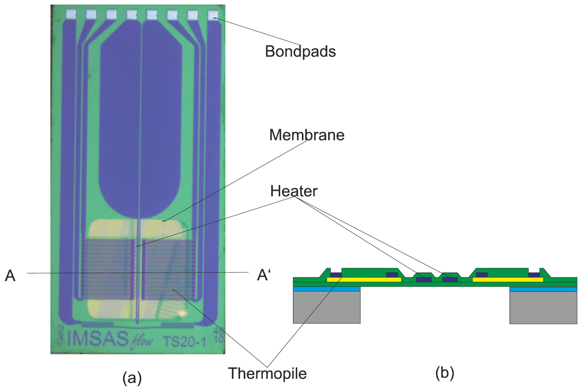
Micro-machined thermal flow sensors are used for many applications, especially ones that need a fast response time such as medical and automotive applications. For example, in the medical field, the respiration disturbances related to some cardiovascular diseases are a supplementary risk for the cardiovascular system. They require urgent diagnostic assessment and consistent therapeutic measures. Thermal flow sensors satisfy such specific requirements of high dynamic flow range and fast response time in controlling the patient's respiration [1]. Therefore, studying and understanding the thermal response time behavior is an important issue for such applications. The thermal flow sensors considered in this study are those developed by IMSAS [2-4]. These sensors are based on silicon as substrate material. They consist of a heater and two thermopiles embedded in a silicon nitride membrane, the thermopiles are placed symmetrically on both sides of the heater. The heater is made of tungsten-titanium, whereas the thermopiles are made of a combination of polycrystalline silicon and tungsten-titanium [2]. The thickness of the membrane is 600 nm and its area is 1 mm × 1 mm. Figure 1(a) shows an example of the referred thermal flow sensors and (b) depicts a cross section in the sensor membrane area. In case of zero flow, the heater generates heat which is distributed uniformly to both sides and no difference in temperature is detected between the thermopiles signals. However, in the case of flow, there is a difference in temperature between the two signals. This difference is related to the value of flow.

Although there is no established method for the response time measurements due to the difficulties of realizing generated defined fluidic steps [3], there are reports about measuring the response time. Some of these reports are: Sosna et al. [3], Ashauer et al. [5], Kohl et al. [6] and de Bree et al. [7]. In the first one, Sosna et al. investigate an electrical measurement of thermal response time and present a model for that measurement. According to this method, an electric heating impulse is applied to the sensor heater which causes a heat transfer through the membrane. The two thermopiles detect a rising in temperature (measured as an electric voltage) that leads to estimate the thermal response time. The disadvantage of Sosna's model is the characterization of the sensor membrane with one temperature value only; which leads to a noticeable difference between the experimental and the model results. The actual work presents a more detailed model in which the membrane is divided into 100 nodes. The temperature of each node is calculated by solving the heat transfer equations through a MATLAB-based modeling program for each time step (1 μs) of the program. Results meet the experimental results of the response time, and provide the sensor output signals (thermopiles) in the steady state case.

2. Description of the Modeling Program

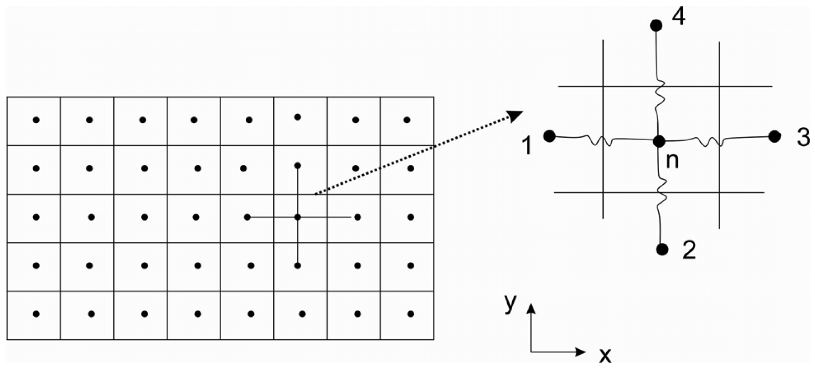
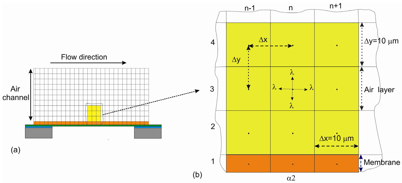
This modeling program uses the numerical analysis approach in order to solve heat transfer equations within the sensor membrane and the surrounding fluid. A cross section in the membrane and the air flow channel represents a two dimensional body with uniform thickness in the z-direction. We assume that there is no temperature gradient in that direction. By choosing appropriate spacing, the body is divided into a network of nodes. Each node is characterized by a single nodal point at its center as shown in Figure 2. It is assumed that the heat transfer occurs between nodal points only.

The formula for the evaluation of temperature in each node based on the explicit Finite-Difference conduction equation [8] is given by:

$$T_n^{t+1}=T_n^t+\Delta t\left[{\sum }_m\frac{T_m^t-T_n^t}{R_{mn}{C}_n}\right]$$

(1)

where m represents all four nodes adjacent to node n in both x and y directions; R_mn is the thermal resistance and C_n is the thermal capacitance:

$$R_{mn}=\{\begin{array}{cc}\frac{\Delta s}{\lambda .A_{k,mn}}& \mathit{\text{for}}\mathit{\text{conduction}}\\ \frac{1}{\alpha .A_{c,mn}}& \mathit{\text{for}}\mathit{\text{convection}}\end{array}$$

(2)

$$C_n=\rho c{V}_n$$

(3)

where Δs is the grid spacing; λ is thermal conductivity; α is the wall heat transfer coefficient; A_k,_mn is the area for conductive heat transfer between nodes m and n; A_c,mn is the area for convective heat transfer between nodes m and n; ρ is the density; c is the specific heat; and V_n is the volume element of node n.

The wall heat transfer coefficient is given by:

$$\alpha =Nu\frac{{\lambda }_{\mathit{\text{air}}}}{l}$$

(4)

where l is the characteristic length and Nu is the Nusselt number. We assume l to be the effective diameter which is defined as:

$$l=4\text{A}/\text{P}$$

(5)

with A the flow cross sectional area, and P the perimeter, respectively. In our case, l is obtained to be 1.2 mm. For the calculation of Nu two different cases are considered. The stagnant air case; where Nusselt number is a constant independent of Reynolds number, Prandtl number, and axial location. This constant value is estimated to be 2 for the chip [9]. By considering the rectangular cross section of the used air channel and by assuming laminar fully developed conditions, the Nusselt number is estimated to be 3.86 [10]. The wall heat transfer coefficient is then equal to 97 W/m²·K for the stagnant air case, but when we have flow the previous conditions are no longer applicable. The Nusselt number is calculated in this case according the following equation [10],

$$Nu=0.664{\mathit{\text{Re}}}^{\stackrel{1}{}/\underset{2}{}}\mathit{\text{Pr}}{}^{\stackrel{1}{}/\underset{3}{}}$$

(6)

where Re is Reynolds number and Pr is Prandtl number.

3. Results and Discussion

3.1. One Dimensional Model for the Response Time

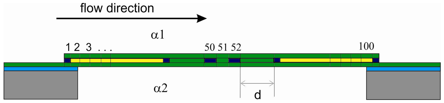
Firstly, a one-dimensional model is established to obtain the thermal response time of the flow sensor. A cross section of the sensor membrane is divided into 100 nodes as shown in Figure 3. These nodes are equal in dimensions but different in their properties i.e., thermal conductivity, density and specific heat capacity according to the constituents of each node. This enables us to precisely calculate the thermal resistance and thermal capacitance for the nodes. The values of the constituents' properties are listed in

Table 1. Properties of constituent's elements.

Element	λ [W/m·K]	cp [J/kg·K]	ρ [kg/m3]
Titanium	20	530	4,500
Tungsten	177	130	19,300
Poly-silicon	34	710	2,300
Silicon Nitride	4	750	3,100
Air	0.03	1,006	1.18

. In this model the time varying conduction in between the membrane nodes is considered, as well as the air convection of both membrane sides.

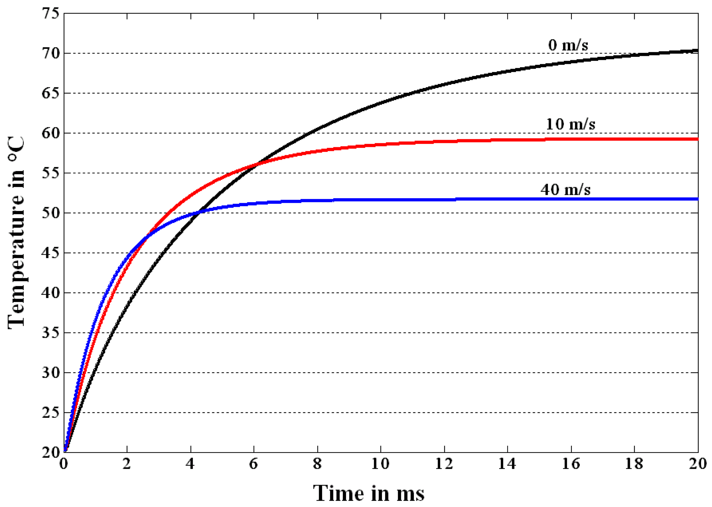
Two sensor configurations are considered regarding the membrane geometry: TS20 and TS50. They have the same membrane area 1 × 1 mm², but differ in the distance d between the heater and the hot contact of the thermopiles as shown in Figure 3. This distance equals 20 μm for TS20 and 50 μm for the sensor TS50. When a step function is given to the heater, this raises its temperature and leads to a heat transfer through the membrane which depends on the material's properties and the air velocity. First, a specified value is set for the air flow velocity. The flow goes through an air channel which is mounted onto the sensor membrane. Then the step function is given to the heater. The temperature of each node is affected by the temperatures of its adjacent nodes, as presented in Equation (1). The program calculates and registers the temperature values every μs for all nodes in the membrane, starting from the instance of applying the impulse to the heater. Figure 4 depicts the temperature curves for the thermopile signals for some air velocity values. Response time is then estimated from these curves, which corresponds to 63.2% of the stable sensor signal amplitude for the chosen velocity. It is necessary to mention that the heat transfer mechanisms for the zero flow case and the one under flow are different. The modeling program differences in calculation between the both cases as described in Section 2. Comparison here is done only to show the response time over the whole studied range.

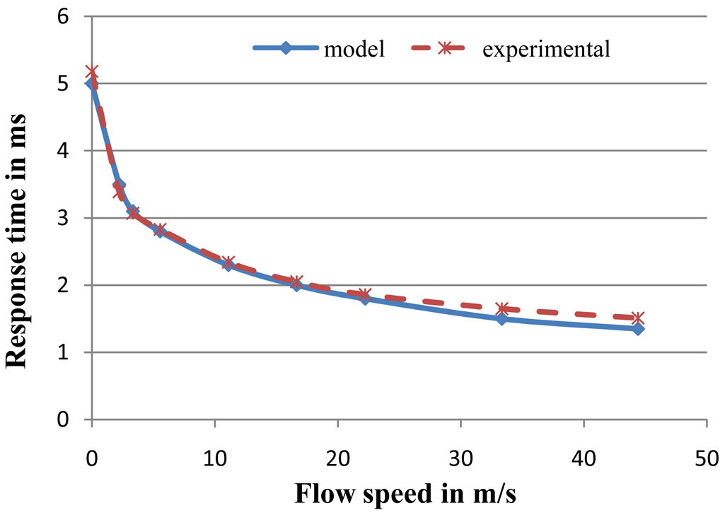
The response time of the configuration sensor TS20 is 5 ms in the stagnant air case. However, in the case when a flow exists, the time constant decreases to ca. 1.5 ms at air velocity of 44 m/s. As the flow increases, the heat transfer between heater and thermopiles rises and the response time is thus reduced. These results are compared with the experimental measurements performed by Sosna et al. [3] for the same sensor configurations and by applying the same conditions. Comparison shows high agreement between the model and the experimental results, especially for the low velocity range, but a slight difference between both results appears from the velocity 20 m/s and becomes larger as the flow speed increases, as presented in Figure 5. This difference could be explained by two arguments. The first argument is the fact that in Equation (6) the flow is assumed to be laminar. However, for velocities higher than 30 m/s the flow enters the transition region, which may cause some errors. The second argument is the fact that heat transfer is assumed to be only in the sensor membrane and the model does not take into account the heat carried by the fluid along the sensor's plane. However, the maximum error is less than 0.2 ms for the studied velocity range.

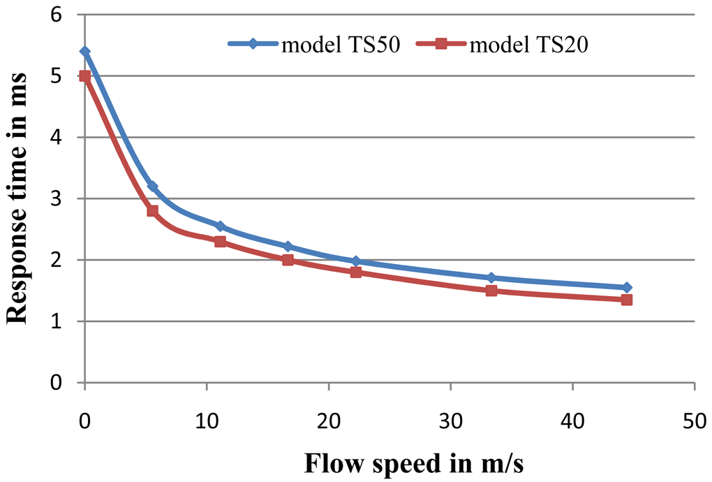
Model results also explain the dependence of the response time on the distance between the thermopiles and the heater. The larger the distance, the higher the response time because heat travels further, as shown in Figure 6, which compares the response times of two sensors (TS20 and TS50).

3.2. Two Dimensional Model for the Steady State

Secondly, another dimension (2D) is added to the previous model, mainly for the steady state case, to be able to model the thermopiles output as a function of flow velocities. The new dimension consists of virtual sublayers of the air flowing over the membrane through the air channel as depicted in Figure 7. In addition, we take into account the conduction among air nodes in both directions x and y, assuming that the air particles flow in straight lines along the air channel.

For each time step, the conduction equations are applied to all nodes, and then each virtual air node moves one step in the direction of the flow to replace the next node. This means we can assume for the sake of simplicity that all layers move at the same speed, which is not true in reality as the velocity should follow a parabolic pattern. Boundary conditions were taken by considering that heat transfer occurs only in the membrane and the air channel; other surroundings keep the same ambient temperature.

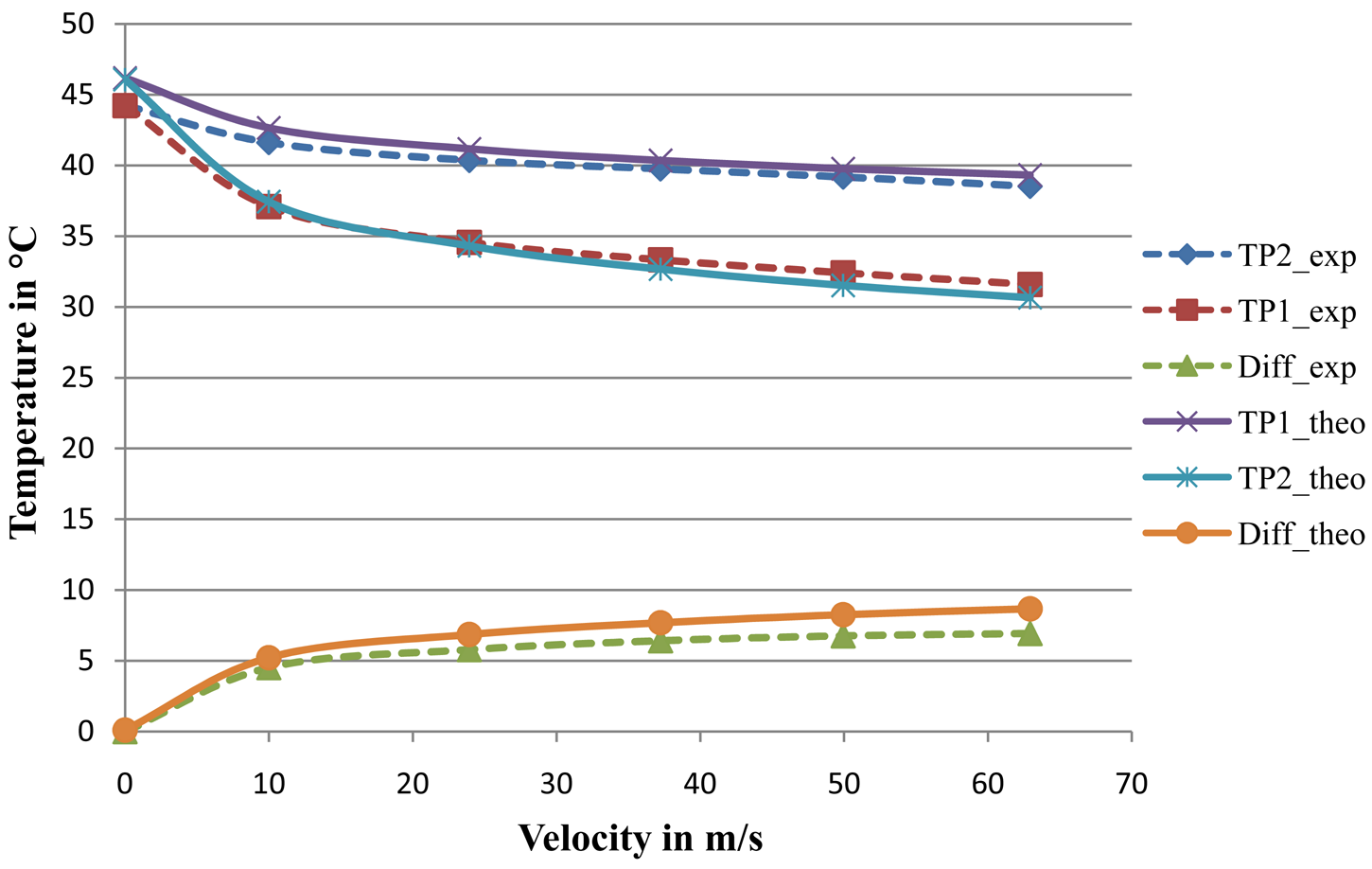
This 2D model is used to provide sensor output signals in the steady state case. In this case the velocity was set to values in the range from 0 to 70 m/s. The up- and downstream thermopile signals are extracted, their difference is calculated and the three of them are plotted as a function of the velocity. At zero flow, the two thermopiles give the same signals. When a flow exists, the difference between the two signals is detected, which increases with the increment of the air velocity, as expected [4,11]. The sensor is operated by constant power mode, because when the flow increases, the temperature of the heater decreases due to force convection, this leads then to a decrease in the thermopile's signals. Figure 8 shows a comparison between experimental and the 2D model results for sensor signals. The difference in results could be explained by the fact that all layers are assumed to move at the same speed, as mentioned above. Moreover, the process of homogeneity of units for both results may produce some errors; thermopiles' signals are extracted experimentally as voltage whereas program results are produced as temperatures. The relationship between the output voltage and the temperature difference for the thermopile case is the Seebeck coefficient. This Seebeck coefficient for the sensor thermopiles is estimated to be 4.3 mV/K [2], and then any deviation from the estimated value may cause additional differences between both results

4. Conclusion

A simple theoretical model for response time of thermal flow sensors was presented. Model results agree with experimental measurements and explain the dependence of the thermal response time on sensor geometry and air velocity.

References

- Hedrich, F.; Kliche, K.; Storz, M.; Billat, S.; Ashauer, M.; Zengerle, R. Thermal flow sensors for MEMS spirometric devices. Sens. Actuat. A: Phys. 2010, 162, 373–378. [Google Scholar]
- Buchner, R.; Sosna, C.; Maiwald, M.; Benecke, W.; Lang, W. A high temperature thermopile fabrication process for thermal flow sensors. Sens. Actuat. A: Phys. 2006, 130-131, 262–266. [Google Scholar]
- Sosna, C.; Walter, T.; Lang, W. Response time of thermal flow sensors with air as fluid. Sens. Actuat. A: Phys. 2011. [Google Scholar] [CrossRef]
- Buchner, R. Hochtemperaturprozess zur Fertigung miniaturisierter thermischer Strömungssensoren und ihre Applikation in Flüssigkeiten; Verlag Dr. Hut: Munich, Germany, 2009. [Google Scholar]
- Ashauer, M.; Glosch, H.; Hedrich, F.; Hey, N.; Sandmaier, H.; Lang, W. Thermal flow sensor for liquids and gases based on combinations of two principles. Sens. Actuat. A: Phys. 1999, 73, 7–13. [Google Scholar]
- Kohl, F.; Fasching, R.; Keplinger, F.; Chabicovsky, R.; Jachimowicz, A.; Urban, G. Development of miniaturized semiconductor flow sensors. Measurement 2003, 33, 109–119. [Google Scholar]
- de Bree, H.-E.; Jansen, H.V.; Lammerink, T.S.J.; Krijnen, G.J.M.; Elwenspoek, M. Bi-directional fast flow sensor with a large dynamic range. J. Micromech. Microeng. 1999, 9, 186–189. [Google Scholar]
- Pitts, D.; Sissom, L. Schaum's Outlines of Theory and Problems of Heat Transfer, 2nd ed.; McGraw-Hill: New York, NY, USA, 1998. [Google Scholar]
- Lang, W. Heat transport from a chip. IEEE Trans. Electron Devices 1990, 37, 958–963. [Google Scholar]
- Incropera, F.P.; DeWitt, D.P. Fundamentals of Heat and Mass Transfer, 5th ed.; John Wiley & Sons: Hoboken, NJ, USA, 2002. [Google Scholar]
- Gianchandani, Y.; Tabata, O.; Zappe, H. Comprehensive Microsystems; Elsevier Science and Technology: Cambridge, UK, 2007. [Google Scholar]
© 2011 by the authors; licensee MDPI, Basel, Switzerland. This article is an open access article distributed under the terms and conditions of the Creative Commons Attribution license (http://creativecommons.org/licenses/by/3.0/).
Share and Cite
Issa, S.; Sturm, H.; Lang, W. Modeling of the Response Time of Thermal Flow Sensors. Micromachines 2011, 2, 385-393. https://doi.org/10.3390/mi2040385
Issa S, Sturm H, Lang W. Modeling of the Response Time of Thermal Flow Sensors. Micromachines. 2011; 2(4):385-393. https://doi.org/10.3390/mi2040385
Chicago/Turabian StyleIssa, Safir, Hannes Sturm, and Walter Lang. 2011. "Modeling of the Response Time of Thermal Flow Sensors" Micromachines 2, no. 4: 385-393. https://doi.org/10.3390/mi2040385