
Quantum Genetic Algorithms for Computer Scientists

Department of Applied Mathematics (Biomathematics), Faculty of Biological Sciences, Complutense University of Madrid, Madrid 28040, Spain
Computers 2016, 5(4), 24; https://doi.org/10.3390/computers5040024
Submission received: 7 July 2016
/
Revised: 2 October 2016
/
Accepted: 11 October 2016
/
Published: 15 October 2016
Abstract
:Genetic algorithms (GAs) are a class of evolutionary algorithms inspired by Darwinian natural selection. They are popular heuristic optimisation methods based on simulated genetic mechanisms, i.e., mutation, crossover, etc. and population dynamical processes such as reproduction, selection, etc. Over the last decade, the possibility to emulate a quantum computer (a computer using quantum-mechanical phenomena to perform operations on data) has led to a new class of GAs known as “Quantum Genetic Algorithms” (QGAs). In this review, we present a discussion, future potential, pros and cons of this new class of GAs. The review will be oriented towards computer scientists interested in QGAs “avoiding” the possible difficulties of quantum-mechanical phenomena.
1. Introduction
In the late 1980s, genetic algorithms [1] achieved enough popularity as a method of optimization and machine learning. During this decade the Nobel Prize-winning physicist Richard Feynman thought the possibility of a quantum computer, a computer that operates using the effects of quantum mechanics. However, it would have to wait some time for the emergence of the exciting idea of designing a genetic algorithm capable of running on a quantum computer. However, is this possible?
Genetic Algorithms (GAs) are search algorithms based on Darwinian natural selection and genetic mechanisms present in organisms [2]. In a simple genetic algorithm (SGA) [1], solutions are encoded in arrays that are referred as chromosomes. Usually, the algorithm begins with an initial population of chromosomes, thus the initial set of solutions, which is randomly generated. Henceforth, the algorithm evolves over and over the population in search of an optimal solution. At each generation the chromosomes in the population are evaluated before selection, obtaining their fitness f values, thus the degree of achievement or goodness of the encoded solution. Immediately after chromosomes are evaluated, the algorithm selects the “parents” or mating pool of the next generation, simulating a concept introduced by Darwin: the survival of the fittest. Once a new generation of offspring chromosomes is obtained, the algorithm simulates genetic mechanisms such as crossover and mutation. However, there are genetic algorithms based on other genetic mechanisms such is the case of bacterial conjugation [3]. These mechanisms are very important in living organisms because they are responsible for the biological variability. In the case of crossover this genetic mechanism takes place during the mating between individuals promoting the population convergence towards sub-optimal solutions present in the search space. Nevertheless, in the case of mutation this genetic mechanism involves a random change that occurs in chromosomes, pushing the population to perform a random walk through the search space. The described steps are shown in Table 1, concluding the search once the SGA meets the termination condition, i.e., the algorithm has found an optimal solution [4]. At present, GAs have many applications in optimization problems, e.g., automated design, quality control, manufacturing systems, software design, financial forecasting, robotics, etc. being widely used in fields either economics, biology, chemistry and many others. However, from a theoretical point of view, is it possible to simulate “Darwinian evolution” in a quantum computer? In 1987 Calvin [5] coined the term “Darwin machine” to refer to a machine (analogous to a Turing machine) which returns as output the result of an iterative process similar to a GA. From a theoretical point of view the architecture of a conventional computer is adequate to implement GAs, and also to simulate from a Darwinian perspective the most important aspects of biological evolution. Consequently, whereas a digital computer can successfully simulate a Darwin machine the possibility to simulate a “Darwin quantum machine” in a quantum computer remains today a controversial question. However, what is known as “Quantum Darwinism” [6] will open up the possibility. Therefore, the Darwin’s concept of survival of the fittest could be simulated in any device capable of data manipulation based on quantum mechanical phenomena [7]. In any case, and without going into theoretical issues, since 1956 [8] when was first proposed the genetic algorithms Evolutionary Computation has made great progress. In 2002 Han [9] introduced a novel evolutionary algorithm inspired by quantum computing, growing from this date the number of publications on quantum-inspired genetic algorithms. In 2010 Ying [10] proposed that quantum computing could be used to achieve certain goals in Artificial Intelligence (AI). Over the last decade, the possibility to emulate a quantum computer has led to a new class of GAs known as “Quantum Genetic Algorithms”. In this review, we present a discussion, future potential, pros and cons of this new class of GAs, including some material presented in a lecture delivered at [11].
2. What is Quantum Computing?
One of the most striking ideas of quantum computing is that as long as a digital computer is a symbolic machine, i.e., an instruction execution engine, a quantum computer is a physical machine. This means that in a quantum computer the hardware-software duality is less obvious than in a classical computer, being the quantum circuit “hardware” itself an isolated “quantum system”. Therefore while in a digital computer a computation is given by the logical operations performed in a “symbolic system”, in a quantum computer a computation is the evolution experienced by the quantum system.
According to quantum mechanics the evolution of an isolated quantum system from an initial state to another final state, e.g., a quantum computer, is governed by the Schrödinger equation:
where i is the imaginary number and is a constant term named “reduced Planck constant”. Planck’s constant plays the role of relating the energy in a photon to frequency, and since frequency is measured in cycles per second it is more convenient to use . According to the mathematical expression the Schrödinger equation is a partial differential equation which “physical variable” is a state vector written in a somewhat special notation that we will discuss later. The vector depends on time and describes the state of a quantum system at time t, in this case the quantum computational state. Since we are dealing with a differential equation, the equation also includes a rate of change or differential term, i.e., . The Schrödinger equation is the holy grail of quantum computing because it characterizes the evolution of a computing state through time. The term H(t) is known as “Hamiltonian operator” and somehow given the initial state it represents the sequence of operations performed by a quantum computer. Establishing a parallelism between quantum and digital computers we assume that quantum state resembles the input of a digital computer. An interesting point is that if we know the Hamiltonian then the Schrödinger equation can be solved, so without going into details we will denominate U(t) as the solution of this equation. Hence, given an initial state the solution of the Schrödinger equation at time t is given by the following linear mapping in the state space:
Therefore and according with the above reasoning we can conclude that in a quantum computer the output is the result of the (i) evolution of the Schrodinger equation and subsequent (ii) measurement (the meaning of measurement in quantum mechanics is introduced later). As may be seen, the equation uses for the state vector a notation that is rather unusual. The reason is because quantum mechanics has its own customized notation for classical vector and matrix operations [12]. In 1930 the theoretical physicist Paul Dirac published the book “The Principles of Quantum Mechanics” introducing the ket notation to refer to a column vector:
and bra notation to denote a row vector:
Hence, the product of a bra and a ket vectors, which is written in the notation of Dirac as follows, is the ordinary inner product:
Alternatively, the product of a ket and bra vectors, is the outer product of the two vectors:
In quantum computing the elements of vectors and matrices are complex numbers but in practice we can ignore this detail.
2.1. Quantum Information
The unit of information in a quantum computer is the quantum bit or qubit, storing and states as well as a linear combination of both states (superposition principle). This linear combination represents a qubit in its “coherent state” or “quantum superposition”, i.e., where and are the qubit amplitudes of the states and . Amplitudes are complex numbers () so the exact state of a qubit is specified by two complex numbers describing the particular combination of 0 and 1 in the superposition state. The normalization of the states to the unit ensures that and therefore , are the probabilities of finding the qubit in or states. According to Dirac notation such superposition is represented in vector form as follows:
and therefore we will represent and states of a qubit:
In the realm of quantum mechanics the states of a qubit are represented geometrically in what is called as Bloch sphere. From a mathematical point of view, the state vector representing the state of a qubit is defined in a space referred as Hilbert space. In a very general sense and without going into details a Hilbert space is a complex vector space with the advantage that allows us to treat a function as a vector, conducting mathematical operations by the simple application of standard algebraic methods. In consequence the quantum computing state which evolution is ruled by Schrödinger equation is defined by a Hilbert space associated with a finite number of n qubits. Despite all these abstract concepts finally the definition of a universal quantum computer is close to the conceptual framework of classical computation [13].
One of the most amazing ideas of quantum mechanics is that any attempt to measure a quantum superposition, or equivalently any interaction of the quantum system with the environment, causes the destruction of the superposition (interference principle). This is a natural phenomenon known in quantum physics as “collapse of wave function ” and represents a major challenge in building a quantum computer. Consequently a measurement or observation of the qubit in its coherent state results in a lost of the superposition, transforming the qubit in a classic decoherent bit, i.e., 0 or 1 state. The interference principle has recently been simulated based on a new class of hybrid cellular automata [14] performing as either a quantum cellular automata (QCA) or as a classical von Neumann automata (CA).
In a quantum computer the input is stored in a quantum memory register:
The register state is the result of Kronecker or tensor product among two or more qubits (operation that is represented with the symbol ) as:
For instance, number 5 is represented in binary numbering system as , being the register state:
However, there are quantum states which cannot be written as a tensor product of two states, being known these special states as entangled states (entanglement principle). In this case, measurement results are dependent as it will occur at the following quantum state:
Once the information is processed by a quantum circuit, the output is the result of a measurement or observation of the qubits states resulting the collapse of wave function . Computation concludes once such measures have been made. In summary, in terms of computing a quantum algorithm maps an input state (or represented for simplicity as ) onto the output or final state (represented as ):
where U (or U(t), the solution of the Schrödinger equation) is referred to as “unitary evolution operator”. An important issue is that U operator can be decomposed in a sequence of q elementary quantum gates (abbreviated as Q-gates) defining these gates a quantum circuit. Q-gates perform unitary transformations on qubits, bearing in their function a resemblance with classical Boolean gates. Consequently from left to right:
A quantum circuit, thus the U decomposition, represents a quantum algorithm being somehow equivalent to a classical algorithm in a digital computer. However, quantum circuits show special features allowing to a quantum computer conduct computations with a lower number of exponential operations than classical computers.
2.2. Quantum Gates
Quantum gates (Q-gates) operate on qubits undergoing unitary transformations being such operations represented by matrices. Since these unitary transformations are rotations in the Bloch sphere then Q-gates are reversible gates. The most important quantum gates that operate with a single qubit are the identity gate I and Pauli gates X, Y and Z:
The identity gate I leaves a qubit unchanged. Pauli X gate performs a Boolean NOT operation, Pauli Y gate maps or and Pauli Z gate changes the phase of a qubit, thus , . For instance, let’s consider the following operations between one of the above quantum gates and or qubit states:
One of the most useful Q-gates is the Hadamard or H gate. This gate is a generalization of the discrete Fourier transform which can be defined recursively for two, three or more qubits:
Let’s be a superposition vector:
multiplying the matrix H by the above vector we obtain:
For example, if we multiply H by we obtain:
or using a different notation (Figure 1). Therefore, if we measure or observe the qubit state then we will have exactly 50% chance of seeing as 0 or 1. Similarly if now we multiply H by we obtain:
or in the alternative notation (Figure 1).
One of the applications of Hadamard gate is the initialization of a quantum register. Generalizing the H gate multiplication by to an n-qubit register that stores the value results in a superposition or mixed state:
It is interesting to note that in the case we could observe the quantum register in the above mixed state then we would see each of the 2n binary numbers x with equal probability.
Of course, there are also Q-gates for two or more qubits operations (e.g., SWAP, CNOT, Toffoli, Fredkin gates, etc.). The SWAP gate swaps two qubits:
Other Q-gates exhibit the special feature of including one or more qubits controlling the operation. These gates are called U-controlled gates, (e.g., CNOT, Toffoli and Fredkin gates). For instance, the CNOT gate (2 qubits) performs according to truth table (Table 2) the operation (Figure 2a). Note that value is observed after performing the measurement.
In contrast, Toffoli gate (3 qubits) conducts the operation (Figure 2b) according to the truth table (Table 3). The gate inverts the state of Q3 when Q1 and Q2 are set to . Note that value is observed after performing the measurement.
Another controlled gate is the Fredkin gate or CSWAP gate (3 qubits). This gate performs a controlled swap operation: if the control qubit state is equal to then it swaps Q1 and Q2 qubits. In summary, the operations conducted by these controlled gates are represented by the following unitary matrices:
Finally, a common element in quantum circuits is termed as oracle. It is a black box function that receives as input n qubits, performs a unitary transformation U and returns the result as output. One of its most important features is that it can measure and modify a quantum state without collapsing the state to a classical state. Furthermore, an oracle could solve a decision problem in linear time on a quantum computer. In the context of the quantum evolutionary algorithms an oracle would play the role of a classical algorithm conducting operations that are specific of a classical computer. The oracle is usually represented as U or in a more specific symbol as O.
In summary, quantum computer operations are ruled by quantum mechanics, data are qubit arrays and operations are reversible and carried out with quantum gates. Such quantum gates are represented by unitary matrices, so that operations are defined by a linear algebra in a Hilbert space. In contrast, a digital computer is governed by classical physics, data are represented by bit sequences (1010001101…) and operations are irreversible and performed by Boolean logic gates (AND, OR, NOT, NAND, etc.).
2.3. Quantum Algorithms and Quantum Circuits
Usually quantum algorithms (e.g., Shor’s algorithm, Grover’s algorithm, Deutsch’s algorithm, etc.) include quantum mechanical phenomena represented in Table 4 (modified from [15]).
In agreement with the main steps described above a quantum algorithm could be represented with a quantum circuit as shown in Figure 3. Thus, there is a correspondence between a quantum algorithm and quantum circuit. The circuit receives the input from the quantum register providing an output as a result of measuring or observing the state of each qubit. Once defined the ends of the circuit, several lines or cables are located in parallel between both ends, placing the quantum gates, oracle etc. (Table 5) according to the quantum algorithm. We will illustrate how a quantum circuit operates with the following example. Consider the EPR (Einstein, Podolsky and Rosen) circuit (Figure 4), one of the classic circuits in quantum computing. Based on this circuit it is possible conduct experiments of quantum teleportation, thus the transfer of quantum information based on entanglement. First, if we look at the left end of the circuit we note that in the top wire there is an H gate while the bottom wire does not have a quantum gate (or equivalently there is an I gate).
Since H and I are located in parallel lines then we perform the Kronecker product between both gates:
obtaining the following matrix:
Second, if we now look at the section of the circuit on the right side there is a CNOT gate connected in series with the wire where we obtained the above matrix. Since both are connected in series then we carry out the inner product or multiplication between matrices, such that:
obtaining the “EPR matrix” shown below:
In practice this means that the EPR circuit is represented by the above matrix. Suppose now that EPR circuit receives as input the following vector state:
The register information will be processed by the quantum circuit simply carrying out the inner product between the EPR matrix and the vector state, obtaining a new vector:
Once we obtained the above vector the output will be the result of measuring or observing the state of each qubit.
2.4. Quantum Computing in Practice
Nowadays the Canadian D-Wave Systems, Inc. is the only commercial company that offers quantum computers [16]. D-Wave One and Two models are adiabatic computers based on Washington 2048-qubit chip. According to this technology a quantum state converge to a solution based on Boltzmann probability distribution:
Since they are adiabatic computers the best performance is obtained for continuous optimization problems. In recent years D-Wave computers have been acquired by Lockeed Martin and Google (shared with NASA) having spent a total 10–15 mill US dollars. Interestingly, although most researchers lack enough money to buy one of these models, it is feasible to emulate a quantum computer on a conventional computer. Is possible to emulate the operations and algorithms characteristic of a quantum computer using a computer with good performance. At present quantum computing emulation could be conducted applying any of the procedures listed below:
2.4.1. Q-Circuit Simulators
Quantum circuit (Q-circuit) simulators are programs including a GUI for designing and evaluating quantum circuits. Some programs—e.g., [17]—include a compiler option to design a gate to be used in larger circuits. To take the first step there are available two good Q-circuit emulators: QCAD [18], a Windows-based environment for quantum computing simulation (see Table 5 and Figure 4) and jQuantum [19], a quantum computer simulation applet.
2.4.2. Q-Programming Languages
Another possibility is the programming of a quantum algorithm using imperative programming languages oriented to quantum computing [20]. A good example of this option is QCL (Quantum Computing Language) [21]—a programming language (Figure 5) for quantum computers developed by Bernhard Ömer. QCL has been applied in a variety of problems, e.g., solving systems of nonlinear equations [22], the implementation of Bernstein-Vazirani algorithm [23], parallelization of quantum gates [24], simulation of Dijkstra’s algorithm [25] and programming quantum genetic algorithms [26].
In the example shown in Figure 5, two qubits are declared with qureg command: a first qubit in a register labeled as u and the second qubit in a register v. Consequently, we have implemented a quantum memory . Following, using the reset command all qubits are forced to state zero, i.e., we reset the quantum state of the machine such that the machine state is empty . After the reset command a Hadamard function H(u) is applied over u and returns it in a quantum superposition. Since it is only an example without practical purpose, next the example illustrates the use of CNot(v,u), i.e., a controlled not gate with a target qubit v and a control qubit u. The gate mentioned flip v if u is in state one. Following, for the second time we reinitiated the quantum memory with reset command. Thereafter, Not(u) gate is applied to u qubit conducting a NOT operation in a similar manner to classical computing. Finally, we perform again a CNot(v,u) operation.
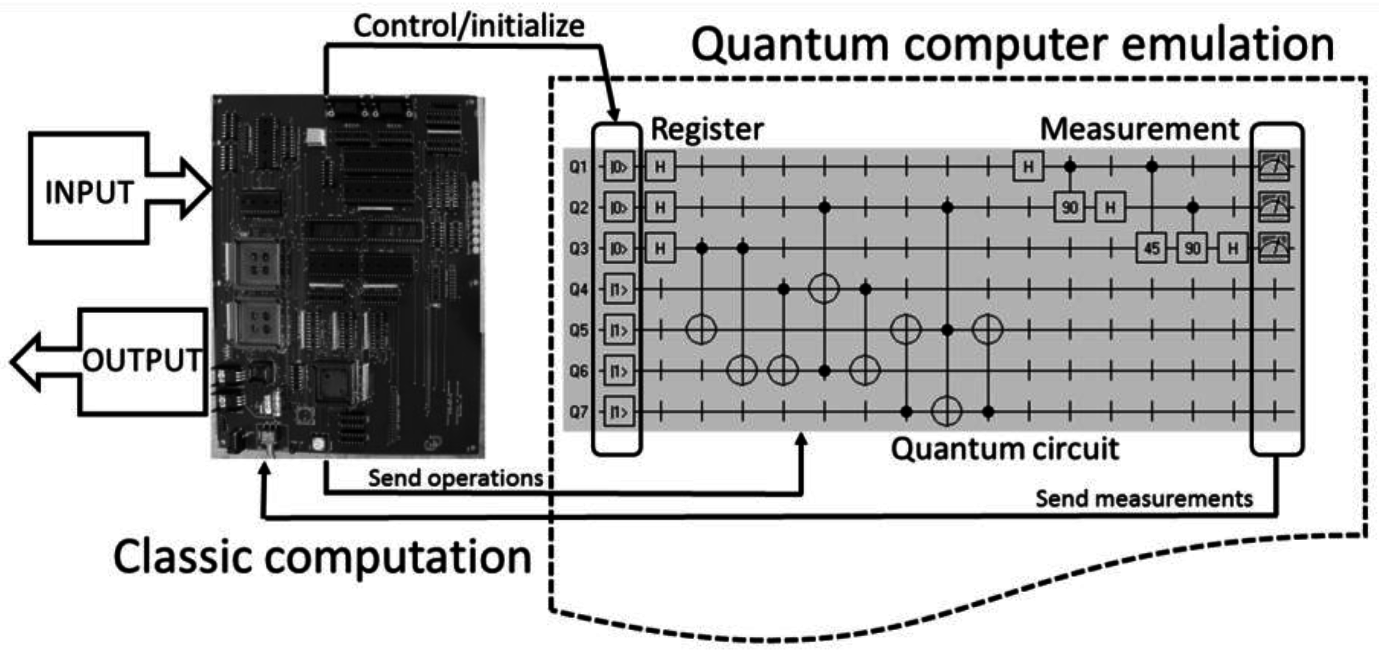
QCL emulates a “Quantum RAM” (QRAM) model (Figure 6), thus a hybrid architecture by which a computer simultaneously performs classical and quantum operations. According to QRAM model the classical computer performs classical computing, controls the quantum register evolution and send the quantum operations to the quantum computer. The quantum computer, which is really simulated on the classic computer, conducts the initialization of the quantum register state, performs unitary transformations and measurements, sending to the classical computer the output. Even when QCL is a fairly representative programming language [27], at present there are other programming languages oriented to quantum computers [28,29,30].
2.4.3. Simulated Q-Computer
Nowadays, programming on a conventional computer under a QRAM environment is the most common option. However, the program can be written in a simulated quantum computer, e.g., Google’s Quantum Computing Playground [31]. A user have accesses to a simulated GPU-accelerated quantum computer with an IDE interface and its own scripting language. The Google’s system has the ability to set quantum registers up to 22 qubits. Using a similar methodology the University of Bristol, Centre for Quantum Photonics (United Kingdom), offers an online quantum photonic chip simulator [32]: an example of quantum computing in the cloud. In this case, the program is written through an IDE showing a circuit, setting the user some photons into the input ports.
2.4.4. Do-It-Yourself: Quantum Computing with Python
Finally, in our opinion, one of the most useful approaches is to write your own program. Using a general purpose language, i.e., Python, we can efficiently implement any quantum algorithm combined with non-quantum computational procedures. Moreover, in the case of Python are available several quantum computing libraries, e.g., PyQu [33], qitensor [34], QuTiP [35], etc. In addition, SymPy [36], a Python library for symbolic computation, includes procedures to perform quantum operations.
3. Quantum Computing and Quantum Evolutionary Algorithms
Since the origins of quantum genetic algorithms (QGAs) [9] until today, lots of QGAs have been proposed in the scientific literature [37,38,39,40,41]. All kinds of quantum evolutionary algorithms have been successfully applied to optimization problems, such as the personnel scheduling problem [42], dynamic economic dispatch problem, e.g., in power systems [43], multi-sensor image registration [44], cryptanalysis [45], etc.
Quantum evolutionary algorithms share the main steps and features of their non-quantum counterparts. In its simplest form and adopting a QRAM architecture (Figure 6) a quantum (or quantum-inspired) evolutionary algorithm consists of the steps shown in Table 6.
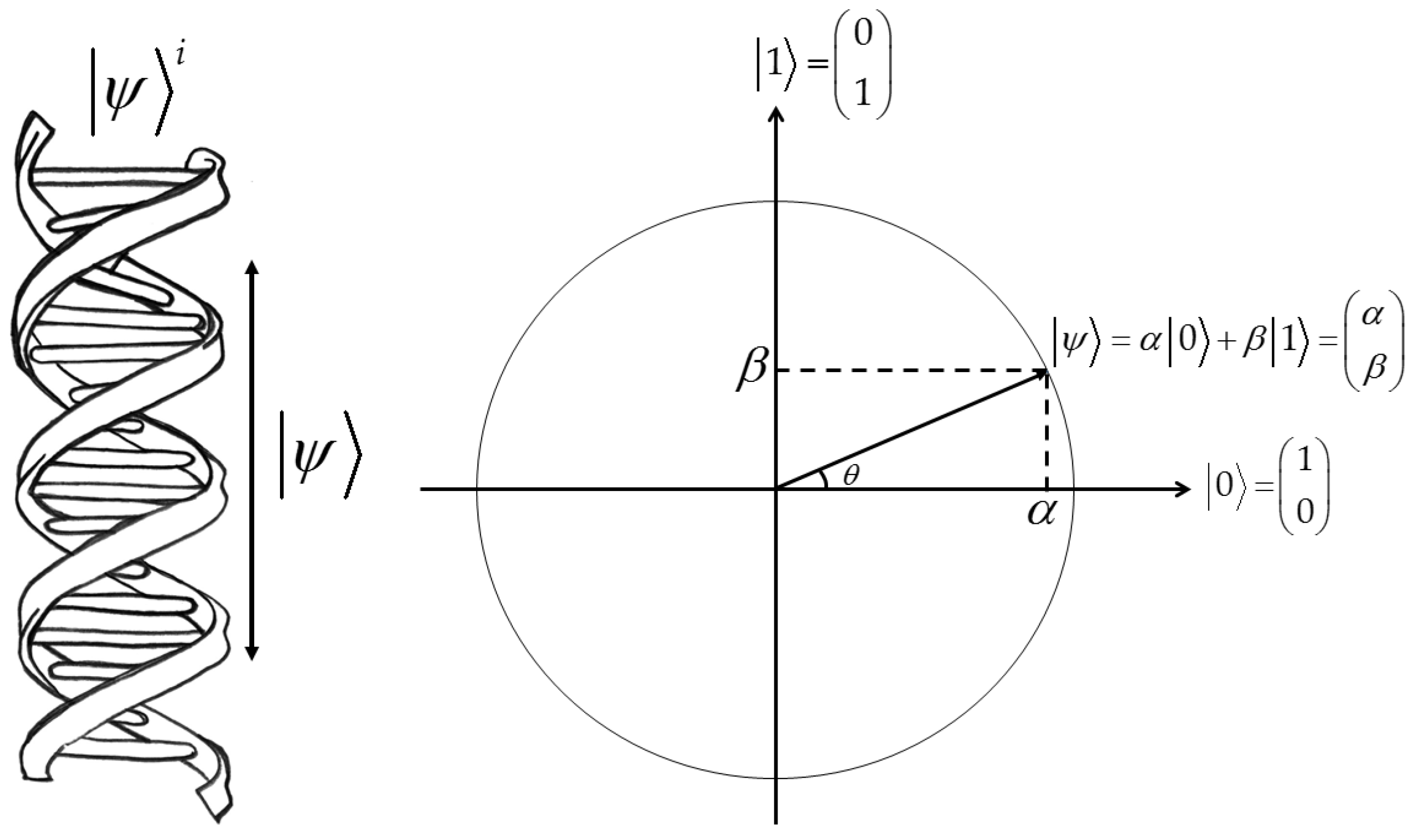
The first step consists in the initialization of a quantum population Q(0) of chromosomes. A quantum chromosome i is defined as a string of j qubits representing a quantum system with simultaneous states:
being the gene j, the qubit represented by vector (Figure 7):
Consequently a quantum population is defined by a set of quantum chromosomes or vectors, as shown below:
The most common technique to initialize the population is to set the value of the amplitudes of all qubits in the chromosomes to a value representing the quantum superposition of all states with equal probability. This is achieved from the product of the Hadamard matrix by the vector :
obtaining a superposition vector. Subsequently to this product a phase angle (0, ] is randomly obtained, being the argument of the trigonometric functions or elements in the rotation matrix U(t):
The initialization step concludes conducting the product of the rotation matrix by the superposition vector, resulting in a pair of amplitudes which define the state of j qubit:
Following, in a second step, we obtain a population P(t) composed of classical chromosomes or bit strings. This population is the result of a measure or observation of qubits states in the quantum chromosomes of the population Q(t). After measurement we get the classical population, such that P(t) is given by a set of vectors:
Qubit observation is simulated, modelling the wave function collapse as follows:
being a random number in the range [0, 1). Assuming we are running the simulation under a QRAM architecture, this step has the purpose to create a population P(t) of classical chromosomes. The aim is to conduct the fitness evaluation on a classical population using a digital computer. Otherwise, fitness evaluation on a quantum computer would produce the collapse of the quantum system destroying the superposition state. The evaluation of fitness is one of the main obstacles in the implementation of QGAs in a quantum computer.
A third step consists in the population update applying Q-gates, thus:
Q(t + 1) = U(t).Q(t)
From a theoretical point of view the evolution of the population is governed by Schrödinger’s equation, being Q-gates the operators that play the role of the “genetic mechanisms” transforming chromosomes. Since evolution takes place in a complex vector space, i.e., a Hilbert space, such transformations are unitary transformations. Thus, let U be a unitary matrix, e.g., a rotation matrix, then it will be a unitary transformation if it holds that U.U’ = I.
In the following section we describe the most characteristic quantum genetic operators.
3.1. Quantum Genetic Operators
At present there are several proposed quantum genetic operators performing genetic operations on quantum chromosomes. It is important to note that in the scientific literature sometimes these operators are termed indifferently like “interference gates” which can confuse the reader. In this review, we have renamed the operators, indicating between parentheses the term interference when in the literature such term is used in reference to such operator.
3.1.1. Qubit (Interference) Rotation Gate
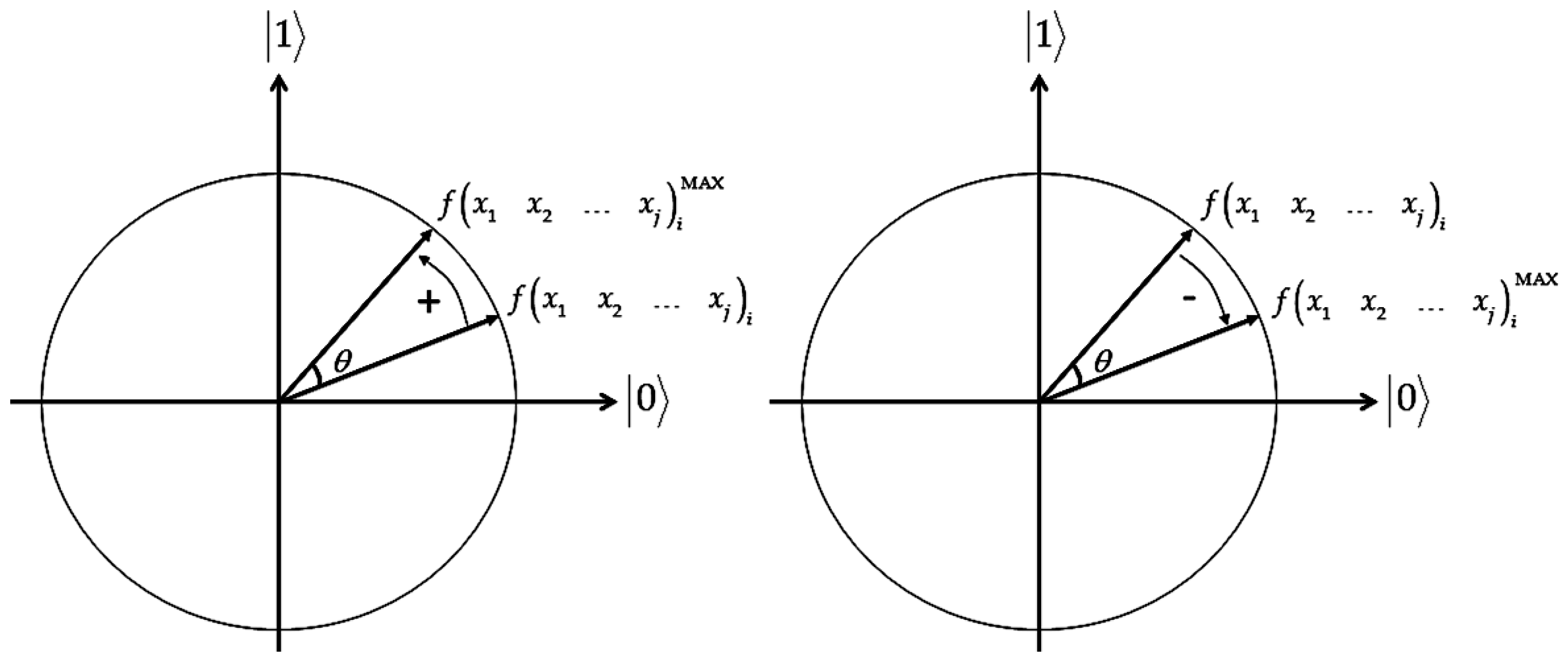
Although there are several updating operators the most characteristic is the interference or rotation Q-gate. The rotation operator or quantum interference is defined as a gate U(t):
Applying this operator the evolution of a population is the result of a process of unitary transformations. In particular, rotations approximating the state of chromosomes to the state of the optimum chromosome in the population. Thus, this gate amplifies or decreases the amplitude of qubits or genes according to the chromosome with maximum fitness . Consequently, the evolution of the quantum state is guided by the best individual (Figure 8):
being and the amplitudes of the j qubit before and after the updating, respectively. In general, the rotation angle is obtained according to the following expression:
where and represent the direction and rotation value, respectively. Note that rotation value plays the role of an “evolution rate”. Consequently, we should avoid too high or too low values. The values of these parameters are summarized in a look-up table (Table 7), comparing the fitness of the current chromosome with the fitness of the best individual .
A disadvantage of rotation operator is that the look-up table depends on the optimization problem, which affects the algorithm performance. Therefore the values in the table should be set according to the optimization problem: e.g., knapsack problem [46,47,48,49], OneMax problem [47], benchmark functions (i.e., De Jong, six-peaks and many-peaks functions) [50]. However, there is a standard table (Table 7) that is usually useful in many optimization problems [51]. In Table 7 is the angle step, having an effect on convergence speed, such that a very large value causes the population converges or diverges very quickly with respect to a local optimum. Unfortunately quantum genetic algorithm performance depends on look-up table values [48], being a general criterion to set values between 0.1 and 0.005 . One common solution is to use an adaptive strategy [37]. For example, suppose we define a range between 0.005 and 0.05 . In this example and according to [52] is changed as:
Note that rotation operator plays the role of the selection operator in SGA. In a classical SGA the selection operator simulates Darwinian natural selection, enhancing populations by promoting individuals with better fitness and punishing those with poorer performance. However, in QGA selection pressure is replaced by a change of all individuals towards the best individual. Therefore, when population is updated with the rotation operator the population converges to the fitter states, but usually QGAs are trapped in local optima undergoing premature convergence. In order to avoid this problem sometimes quantum genetic algorithms include either roulette or elite selection. For instance, a QGA with a selection step is used in an improved K-means clustering algorithm [53]. In fact, there are more extreme approaches such as [54] where a QGA includes selection and simulated annealing avoiding premature convergence. In other cases a selection step is included without resorting to operators commonly used in SGAs. Such is the case of a semiclassical genetic algorithm [55] where a selection operator seeks for the maximum fitness individual by means of a quantum approach, in particular using a variant of the Grover’s search algorithm.
3.1.2. Quantum Mutation (Inversion) Gate
In imitation of SGAs there is also available a quantum version of the classic mutation operator [57]. The gate performs an inter-qubit mutation of the jth qubit, swapping the amplitudes with the quantum Pauli X gate:
resulting in:
3.1.3. Quantum Mutation (Insertion) Gate
This gate [57,58] reminds the biological mechanism for chromosome insertion. Chromosome insertion means that a chromosome segment has been inserted into an unusual position on the same or different chromosome. The quantum version of this genetic mechanism involves the permutation or swap between two randomly chosen qubits (left qubit, right qubit). For example, suppose that given the following chromosome we choose randomly the first and third qubits:
once applied the insertion operator, we get the new chromosome:
3.1.4. Quantum Crossover (Classical) Gate
Quantum crossover [57] is simulated resembling the classical recombination algorithm used in SGAs but operating with amplitudes. However, whereas the quantum version of mutation could be implemented on a quantum computer, there are theoretical reasons preventing this with crossover. Nevertheless, and despite the theoretical limitations, the quantum version of classical crossover operator is applied in many practical optimization problems. In these cases a solution is searched using a quantum evolutionary “inspired” approach. Following, the operator is illustrated for the case of one point crossover. In this example if the cut point is randomly chosen, e.g., a point between first and second positions, then an exchange of chromosomal segments occurs:
resulting the following recombinant chromosomes:
3.1.5. Quantum Crossover (Interference) Gate
The present quantum operator [59] performs crossover by recombining according to a criterion based on drawing diagonals. In consequence, all individuals interfere with each other resulting the offspring. Consider the following example. When the crossover is performed with the next six chromosomes:
we obtain the following first and second recombinant chromosomes:
3.2. A Canonical Classification of Quantum Evolutionary Algorithms
In order to summarize this review as much as possible, most of the quantum evolutionary algorithms have been grouped into two major classes: Quantum Genetic Algorithms (QGAs) and Hybrid Genetic Algorithms (HGAs). Since there is no agreement on terminology, different names are used interchangeably: Quantum Evolutionary Algorithms (QEAs), Quantum-Inspired Evolutionary Algorithms (QIEAs), etc. Anyway, in general a QGA includes the main steps shown in Table 8. Likewise an HGA comprises the main steps set out in Table 9.
4. Towards True Quantum Evolutionary Algorithms
QGA and HGA algorithms can be considered as classical optimization methods inspired by the principles of quantum computing. Programs implementing such methods can be executed on a digital computer, without this implying practical or theoretical difficulties. At present one of the challenges in Quantum Artificial Intelligence is the design of true quantum evolutionary algorithms and therefore of programs that in the future can run on a quantum computer. However, some problems arise when we translate the main steps of a SGA to the quantum version. This is a paradoxical situation because a SGA bears a resemblance to Grover’s quantum algorithm: SGAs are parallel search methods although this feature is not implemented in their usual applications. One of the main problems with QGA and HGA algorithms [60] is to find a method to perform measurements of the population of individuals but without collapsing the superposition state of chromosomes. Furthermore, [60] notes that to date a key issue not addressed is how to implement in a quantum computer a crossover operator. Whereas mutation could be easily conducted in a quantum computer, i.e., using a Pauli X gate, it is unclear how to carry out crossover using for this purpose quantum mechanical phenomena.
One of the most interesting ideas is proposed in 2006 by [61,62] taking the first steps in the implementation of a genetic algorithm on a quantum computer. The authors of these papers proposed a true quantum evolutionary algorithm, which was termed as Reduced Quantum Genetic Algorithm (RQGA). The algorithm consists of the main steps described below (Table 10).
In the first place, the algorithm begins preparing a superposition of all individuals, i.e., N, or chromosomes of population Q(t):
Therefore, all individuals are represented by only one individual quantum register. That is, the entire population is represented by a single chromosome in a superposition state:
One of the key steps of RQGA is the correlation between the individual quantum register and a fitness quantum register :
From a formal point of view, we have a fitness quantum gate F which evaluates the fitness of individuals (Figure 9). In 2008 [63], a similar idea is also applied to other version of a true quantum evolutionary algorithm which was termed as Quantum Genetic Optimization Algorithm (QGOA).
In a second step the algorithm searches for the maximum fitness:
In the late 1990s, [64] proposed a quantum algorithm for searching the maximum value among N values. Once the operator F is applied, RQGA searches for the maximum fitness value based on the Grover’s search algorithm [65]. This is one of the most popular quantum algorithms oriented to search in an unstructured database. Without going into details on this algorithm, RQGA performs the following two steps. First, given a register with a set of fitness values an oracle O is designed to mark all the kets:
having a fitness value greater than a cutoff value:
such that:
Secondly, the algorithm concludes applying Grover’s diffusion operator G. This operator aims at finding the marked states, i.e., :
Finally, making a measure in the chromosome with maximum fitness is obtained. All these steps are summarized in the quantum circuit shown in Figure 10.
5. Simulation Experiments
In this review, we illustrate how to implement the above quantum genetic algorithms, using a simple optimization problem. The goal is to find the value of x within the range that maximizes the value of the benchmark function shown below:
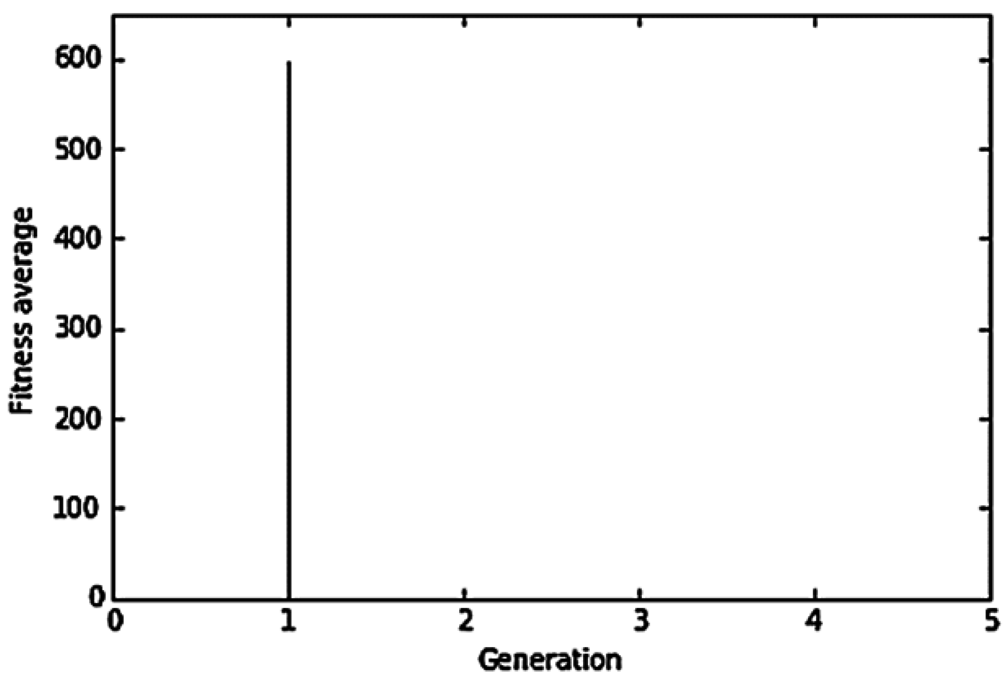
The f(x) function has an optimum reached with x = 11, thus 1011 in binary numbering system. Since in the experiments f(x) is multiplied by 100, the maximum fitness is equal to 599.9941. QGA, HGA and RQGA codes were written in Python 3.4.4 language and they can be downloaded from [66,67,68]. In the simulation experiments conducted with QGA we defined three experimental protocols: QGA in the absence of mutation (QGA1), QGA setting population and qubit mutation probabilities equal to 0.01 (QGA2) and QGA setting these parameters to lower values, in particular equal to 0.001 (QGA3). In HGA one-point crossover probability was set equal to 0.75, also conducting three kinds of experiments: simulation experiments in the presence of mutation, i.e., setting population and qubit mutation probabilities equal to 0.01 (HGA2) and setting these parameters to 0.001 (HGA3). As in the previous experiments with QGA we also conducted simulation experiments without mutation (HGA1). The simulation experiments conducted with above quantum genetic algorithms were compared with a non-quantum simple genetic algorithm (SGA). The SGA code can be downloaded from [69]. In this latter algorithm the one-point crossover probability was equal to 0.75 and the population and bit mutation probabilities were both equal to 0.01. Simulations were performed for 150 generations, with a population size of 50 chromosomes. Thereafter, we performed five experimental replicates with each of the above algorithms. Next, from each experimental replicate we selected the average fitness values from the last 10 generations. Finally, for each of the algorithms a total of 50 values (5 replicates × 10 fitness averages) was collected in a single sample. Statistical analysis [70] of the seven samples (SGA, HGA1, HGA2, HGA3, QGA1, QGA2 and QGA3) was accomplished using the statistical package STATGRAPHICS Centurion XVII version 17.1.12 (Statpoint Technologies, Inc. Warrenton, VA, USA).
6. Results
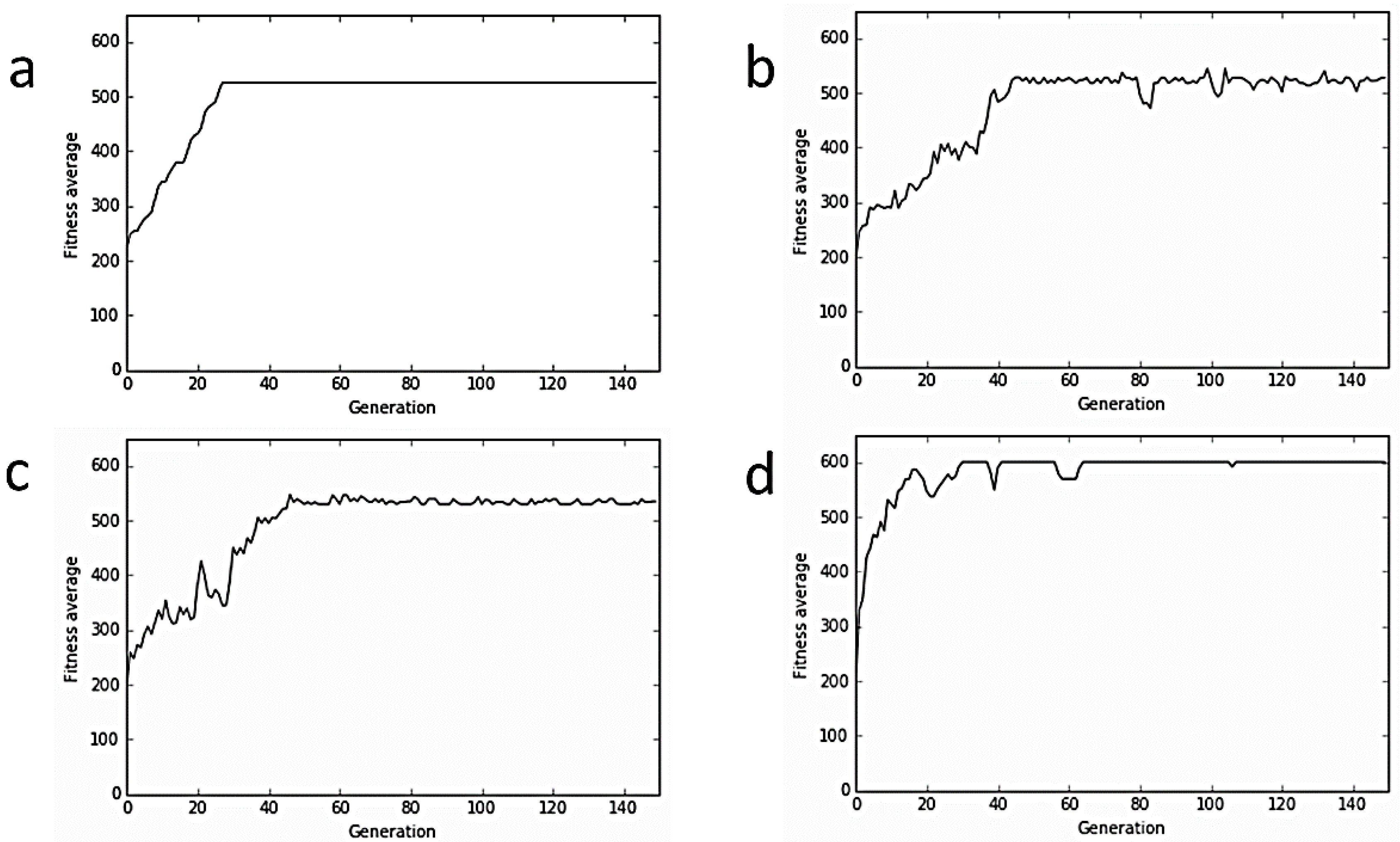
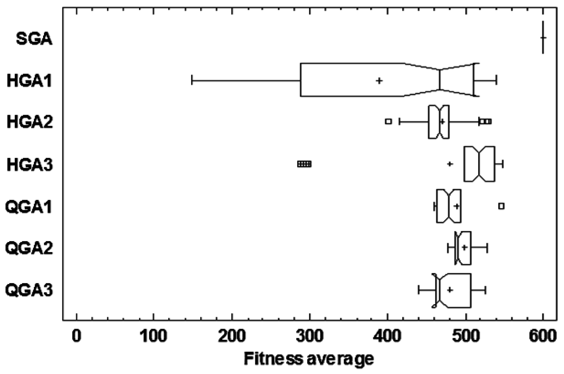
The obtained results show how the classical algorithm SGA has greater performance than the quantum versions of the genetic algorithm (Figure 11). In fact, SGA is the only evolutionary algorithm that achieves the maximum value of fitness, i.e., 599.9941 (Figure 12). The Kruskal-Wallis test (Table 11) shows with a p-value equal to zero that there are statistically significant differences among medians at the 95.0% confidence level. Compared to each other the algorithms we conclude that SGA differs significantly from HGA and QGA. The HGA algorithm without mutation (HGA1) differs significantly from HGA with mutation (HGA3), whereas there are not significant differences among the QGA protocols. One possible explanation for the better performance of SGA could be the mechanism that drives evolution. That is, in QGA and HGA evolution is the result of unitary transformations, particularly rotations approximating the state of chromosomes to the state of the optimum chromosome with maximum fitness. Since this procedure is repeated generation after generation the result is a fast convergence to local optima, taking place a phenomenon of local trapping. A general strategy to improve QGA performance consists of using minor enhancements of the algorithm. For instance, including new operators, e.g., a quantum disaster [56], perturbation [71] or other “customized” algorithms [72]. In many cases, these operators are only useful in highly specific applications, e.g., in Bioinformatics specific quantum operators (ResidueBlockShuffle, GapBlockShuffle, BlockMove, etc.) were devised by their authors [73] in a problem of multiple sequence alignment.
Therefore, we could conclude that in quantum evolutionary algorithms evolution (or optimization) is the result of a rotation quantum gate, which introduces an interference phenomenon. Thus, individuals are adjusted or modified to be more similar to the best individual in the population. Consequently, the population is subjected to a lower Darwinian selection pressure. However, in SGA once individuals are evaluated the algorithm simulating selection (e.g., wheel parents selection operator) will replace the old population P(t) with a new population P(t + 1) of individuals. Since individuals are selected according to their fitness values we are evolving a population of solutions via Darwinian evolution but with a greater selection pressure than QGA and HGA. Hence, SGA replaces obsolete strategies by innovative strategies represented by the offspring. Likewise, when crossover is included as a step in HGA algorithm, its performance usually improves approaching to SGA.
An advantage of the quantum genetic algorithms is that they require fewer chromosomes than SGA. Under a theoretical realm in a “true” quantum genetic algorithm, i.e., RQGA, we can consider that the population is made up of a single chromosome in a state of superposition. Although this fact may be bizarre at first sight, it is not from the perspective of quantum mechanics. Moreover, the algorithm RQGA demonstrates that using quantum computing the genetic search strategy becomes unnecessary (Figure 13): evolution takes place in a single generation.
In order to illustrate above idea let us consider the results we have obtained once the RQGA program was executed on a “quantum computer”. First, the program creates the superposition state:
In second place, the oracle O marks the maximum fitness of :
such that when is applied we obtain the superposition shown below:
This second step is repeated a given number of iterations. The Grover’s maximum number of iterations is calculated as:
being n the number of qubits or length of the quantum chromosome, thus n = 4 in the example of the function described in Section 5. Repeating the second step resulted in:
In third and last place the Grover’s diffusion operator G finds the chromosome in with a marked state. Therefore, performing the following operation the result is:
Finally, making a measure in we get the state that points to chromosome with maximum fitness:
In other words, in the present example we have 15 possible chromosomal states represented as:
Consequently, since RQGA algorithm found the state then according to Table 12 the optimum chromosome is with fitness .
7. Future Directions
Over the next years the incorporation of quantum computing in Artificial Intelligence will lead to a fast development of related research areas, e.g., machine learning, as a consequence of an increased execution speed and effectiveness of the algorithms. For instance [74] report an experimental implementation of a quantum support vector machine algorithm for an optical character recognition problem. In the experiments, they implemented a 4 qubit processor using the NMR technique with 13C-iodotrifluroethylene and a spectrometer at 306 K. Furthermore, in the future we will achieve the physical realization [75] of 50–100 qubits and therefore the hardware to build a quantum computer. At present, it is possible to experience with a 5 qubits quantum computer via a cloud computing platform and run experiments, such is the case of IBM’s quantum processor [76]. However, today, even when QGAs are inspired by principles of quantum computing they are eventually executed on a classical computer. In our opinion this scenario will change once we achieve the design and implementation of a RQGA on a quantum computer. Consequently, this will accelerate research on quantum evolutionary algorithms designing higher-order QGA [77], QGAs with entanglement [78] or hybridizing QGAs with the quantum version of optimization algorithms, e.g., artificial bee colony [79], cuckoo search [58], etc. The leap from emulation to the actual implementation of quantum algorithms is a big step that should be accompanied by a good training of future computer scientists on the fundamentals of quantum mechanics [80]. The result of these changes will be a dramatic increase of the applications of quantum evolutionary algorithms, either on specific problems, e.g., the analysis of cancer microarray data [81] or in classical engineering optimization problems [82]. Moreover, it is also expected an increase in the number of applications in the field of Artificial Intelligence, e.g., the N-Queens problem [83], and even in the field of Artificial Life [84]. In the future quantum computing may also have a profound influence on Darwinism [85], transforming our vision of life on Earth. However, until these advancements occur we must exploit the advantages that provides us the current software and hardware technologies, e.g., designing more efficient QGAs with the support of CUDA (from NVIDIA) platform and the Matlab Graphic Processing Unit (GPU) library [86].
8. Conclusions
In this paper, we survey the main concepts in quantum computing and quantum evolutionary computation. In recent years, the possibility to emulate a quantum computer has led to a new class of GAs, i.e., QGAs. At present, in this class of algorithms research is splitted between two trends or flavors. On the one hand, some researchers are “inspired” by quantum mechanics developing a new class of GAs. In this case, the researcher does not intend in the near future to run the algorithm in a quantum computer. The aim is to solve an optimization problem on a digital computer, either to test a novel improvement or hardware technology in the QGA, or solve real-world problems using a novel class of algorithm instead classical GAs. In our opinion, at present this is the main trend in research on QGAs. On the other hand, in recent years there has arisen a line of research that explores the possibility to design a “true” QGA, so that in the future the algorithm can be run on a quantum computer. According to the way of thinking we have followed through this paper, we believe that this last line of research may have a profound influence on Artificial Intelligence and Artificial Life as well as in disciplines such as Biology.
Acknowledgments
I would like to express my special thanks of gratitude to Dr. Gabriela Ochoa at the Department of Computing Science and Mathematics, University of Stirling, Scotland, for her advice and comments about my research work during my stay in the summer of 2015. R. Lahoz-Beltra was supported by a grant PRX14/00319 from Ministerio de Educación, Cultura y Deporte (Spain) through the program “Estancias de movilidad de profesores e investigadores seniores en centros extranjeros de enseñanza superior e investigación, incluido el Programa Salvador de Madariaga 2014”.
Conflicts of Interest
The author declares no conflict of interest.
References
- Goldberg, D.E. Genetic Algorithms in Search, Optimization, and Machine Learning; Addison-Wesley: Reading, MA, USA, 1989; pp. 1–432. [Google Scholar]
- Lahoz-Beltra, R. Bioinformática: Simulación, Vida Artificial e Inteligencia Artificial; Ediciones Díaz de Santos: A Coruña, Spain, 2004; pp. 237–323. (In Spanish) [Google Scholar]
- Perales-Gravan, C.; Lahoz-Beltra, R. An AM radioreceiver designed with a genetic algorithm based on a bacterial conjugation genetic operator. IEEE Trans. Evolut. Comput. 2008, 12, 129–142. [Google Scholar] [CrossRef]
- Ribeiro Filho, J.L.; Treleaven, P.C.; Alippi, C. Genetic-algorithm programming environments. IEEE Comput. 1994, 24, 28–43. [Google Scholar] [CrossRef]
- Calvin, W.H. The brain as a Darwin machine. Nature 1987, 330, 33–34. [Google Scholar] [CrossRef] [PubMed]
- Zurek, W. Quantum Darwinism. Nat. Phys. 2009, 5, 181–188. [Google Scholar] [CrossRef]
- Feynman, R.P. Simulating physics with computers. Int. J. Theor. Phys. 1982, 21, 467–488. [Google Scholar] [CrossRef]
- Fraser, A.S. Simulation of genetic systems by automatic digital computers. Aust. J. Biol. Sci. 1957, 10, 484–491. [Google Scholar] [CrossRef]
- Han, K.-H.; Kim, J.-H. Quantum-inspired evolutionary algorithm for a class of combinatorial optimization. IEEE Trans. Evolut. Comput. 2002, 6, 580–593. [Google Scholar] [CrossRef]
- Ying, M. Quantum computation, quantum theory and AI. Artif. Intell. 2010, 174, 162–176. [Google Scholar] [CrossRef]
- Lahoz-Beltra, R.; University of Stirling, Computing Science and Mathematics School of Natural Sciences, Stirling, Scotland, United Kingdom. Quantum Genetic Algorithms for Computer Scientists. Computing Science Seminars, Spring 2015, 26 June. Personal communication, 2015. [Google Scholar]
- Susskind, L.; Friedman, A. Quantum Mechanics: The Theoretical Minimum; Penguin Books: London, UK, 2015; pp. 1–364. [Google Scholar]
- Boghosian, B.M.; Taylor, W., IV. Simulating quantum mechanics on a quantum computer. Phys. D 1998, 120, 30–42. [Google Scholar] [CrossRef]
- Alfonseca, M.; Ortega, A.; de La Cruz, M.; Hameroff, S.R.; Lahoz-Beltra, R. A model of quantum-von Neumann hybrid cellular automata: Principles and simulation of quantum coherent superposition and decoherence in cytoskeletal microtubules. Quantum Inf. Comput. 2015, 15, 22–36. [Google Scholar]
- Zeiter, D. A Graphical Development Environment for Quantum Algorithms. Master’s Thesis, Department of Computer Science, ETH Zurich, Zürich, Switzerland, 3 September 2008. [Google Scholar]
- Quantum Computing. How D-Wave Systems Work. Available online: http://www.dwavesys.com/quantum-computing (accessed on 1 July 2016).
- Quantum Circuit Simulator. Available online: http://www.davyw.com/quantum/ (accessed on 25 April 2016).
- QCAD: GUI Environment for Quantum Computer Simulator. Available online: http://qcad.osdn.jp/ (accessed on 25 April 2016).
- jQuantum—Quantum Computer Simulation Applet. Available online: http://jquantum.sourceforge.net/jQuantumApplet.html (accessed on 25 April 2016).
- Hayes, B. Programming your quantum computer. Am. Sci. 2014, 102, 22–25. [Google Scholar] [CrossRef]
- QCL—A Programming Language for Quantum Computers. Available online: http://tph.tuwien.ac.at/~oemer/qcl.html (accessed on 25 April 2016).
- Al Daoud, E. Quantum computing for solving a system of nonlinear equations over GF(q). Int. Arab J. Inf. Technol. 2007, 4, 201–205. [Google Scholar]
- Arustei, S.; Manta, V. QCL implementation of the Bernstein-Vazirani algorithm. Bul. Inst. Politech. Din Iasi 2008, 54, 35–44. [Google Scholar]
- Glendinning, I.; Ömer, B. Parallelization of the General Single Qubit Gate and CNOT for the QC-lib Quantum Computer Simulator Library. In Proceedings of the PPAM 2003, Czestochowa, Poland, 7–10 September 2003; Wyrzykowski, R., Dongarra, J., Paprzycki, M., Wasniewski, J., Eds.; Volume 3019, pp. 461–468.
- Ray, P. Quantum simulation of Dijkstra’s algorithm. Int. J. Adv. Res. Comput. Sci. Manag. Stud. 2014, 2, 30–43. [Google Scholar]
- Yingchareonthawornchai, S.; Aporntewan, C.; Chongstitvatana, P. An Implementation of Compact Genetic Algorithm on a Quantum Computer. In Proceedings of the 2012 International Joint Conference on Computer Science and Software Engineering (JCSSE), Bangkok, Thailand, 30 May–1 June 2012; pp. 131–135.
- Introduction to Quantum Computing. A Guide to Solving Intractable Problems Simply. Available online: http://www.ibm.com/developerworks/library/l-quant/ (accessed on 24 February 2016).
- Quantum Programming Language. Available online: https://quantiki.org/wiki/quantum-programming-language (accessed on 24 February 2016).
- Adam Miszczak, J. High-Level Structures for Quantum Computing; Morgan & Claypool: San Rafael, CA, USA, 2012. [Google Scholar]
- Rüdiger, R. Quantum programming languages: An introductory overview. Comput. J. 2007, 50, 134–150. [Google Scholar] [CrossRef]
- Google’s Quantum Computing Playground. Available online: www.quantumplayground.net (accessed on 26 April 2016).
- Quantum in the Cloud. Available online: http://cnotmz.appspot.com/ (accessed on 26 April 2016).
- Quantum Computing Simulation in Pure Python. Available online: https://code.google.com/archive/p/pyqu/ (accessed on 26 April 2016).
- Qitensor: A Quantum Information Module for Python. Available online: https://github.com/dstahlke/qitensor (accessed on 26 April 2016).
- QuTiP: Quantum Toolbox in Python. Available online: http://qutip.org/ (accessed on 26 April 2016).
- Cugini, A. Quantum Mechanics, Quantum Computation, and the Density Operator in SymPy. Available online: http://digitalcommons.calpoly.edu/physsp/38/ (accessed on 26 April 2016).
- Han, K-H. Quantum-inspired evolutionary algorithms with a new termination criterion, gate, and two-phase scheme. IEEE Trans. Evolut. Comput. 2004, 8, 156–169. [Google Scholar]
- Zhang, G. Quantum-inspired evolutionary algorithms: A survey and empirical study. J. Heuristics 2011, 17, 303–351. [Google Scholar] [CrossRef]
- Roy, U.; Roy, S.; Nayek, S. Optimization with quantum genetic algorithm. Int. J. Comput. Appl. 2014, 102, 1–7. [Google Scholar]
- Sun, Y.; Xiong, H. Function optimization based on quantum genetic algorithm. Res. J. Appl. Sci. Eng. Technol. 2014, 7, 144–149. [Google Scholar]
- Zhifeng, Z.; Hongjian, Q. A New Real-Coded Quantum Evolutionary Algorithm. In Proceedings of the 8th WSEAS International Conference on Applied Computer and Applied Computational Science, Hangzhou, China, 20–22 May 2009; pp. 426–429.
- Wang, H.; Li, L.; Liu, J.; Wang, Y.; Fu, C. Improved quantum genetic algorithm in application of scheduling engineering personnel. Abstr. Appl. Anal. 2014, 2014, 1–10. [Google Scholar] [CrossRef]
- Lee, J.-C.; Lin, W.-M.; Liao, G.-C.; Tsao, T.-P. Quantum genetic algorithm for dynamic economic dispatch with valve-point effects and including wind power system. Electr. Power Energy Syst. 2011, 33, 189–197. [Google Scholar] [CrossRef]
- Talbi, H.; Draa, A.; Batouche, M. A novel quantum-inspired evolutionary algorithm for multi-sensor image registration. Int. Arab J. Inf. Technol. 2006, 3, 9–15. [Google Scholar]
- Hu, W. Cryptanalysis of TEA using quantum-inspired genetic algorithms. J. Softw. Eng. Appl. 2010, 3, 50–57. [Google Scholar] [CrossRef]
- Han, K.-H.; Kim, J.-H. Introduction of Quantum-Inspired Evolutionary Algorithm. In Proceedings of the 2002 FIRA Robot World Congress, Seoul, Korea, 26–28 May 2002; pp. 243–248.
- Laboudi, Z.; Chikhi, S. A Retroactive Quantum-Inspired Evolutionary Algorithm. In Proceedings of the Arab Conference on Information and Technology ACIT 2010, Benghazi, Lybia, 15–17 December 2010.
- Laboudi, Z.; Chikhi, S. Comparison of genetic algorithm and quantum genetic algorithm. Int. Arab J. Inf. Technol. 2012, 9, 243–249. [Google Scholar]
- Han, K.-H.; Kim, J.-H. Genetic Quantum Algorithm and Its Application to Combinatorial Optimization Problem. In Proceedings of the 2000 Congress on Evolutionary Computation, La Jolla, CA, USA, 16–19 July 2000; pp. 1354–1360.
- Ma, S.; Jin, W. A New Parallel Quantum Genetic Algorithm with Probability-Gate and Its Probability Analysis. In Proceedings of the 2007 International Conference on Intelligent Systems and Knowledge Engineering (ISKE 2007), Chengdu, China, 15–16 October 2007.
- Junan, Y.; Bin, L.; Zhenquan, Z. Research of quantum genetic algorithm and its application in blind source separation. J. Electron. 2003, 20, 62–68. [Google Scholar]
- Hang, B.; Jiang, J.; Gao, Y.; Ma, Y. A Quantum Genetic Algorithm to Solve the Problem of Multivariate. In Information Computing and Applications, Proceedings of the Second International Conference ICICA 2011, Qinhuangdao, China, 28–31 October 2011; Liu, C., Chang, J., Yang, A., Eds.; Springer: Berlin/Heidelberg, Germany, 2011; pp. 308–314. [Google Scholar]
- Xiao, J.; Yan, Y.; Lin, Y.; Yuan, L.; Zhang, J. A Quantum-Inspired Genetic Algorithm for Data Clustering. In Proceedings of the IEEE World Congress on Computational Intelligence Evolutionary Computation, 2008, CEC 2008, Hong Kong, 1–6 June 2008; pp. 1513–1519.
- Shu, W.; He, B. A Quantum Genetic Simulated Annealing Algorithm for Task Scheduling. In Advances in Computation and Intelligence, Proceedings of the Second International Symposium ISICA 2007, Wuhan, China, 21–23 September 2007; Kang, L., Liu, Y., Zeng, S., Eds.; Lecture Notes in Computer Science. Springer: Berlin/Heidelberg, Germany, 2007; Volume 4683, pp. 169–176. [Google Scholar]
- SaiToh, A.; Rahimi, R.; Nakahara, M. A quantum genetic algorithm with quantum crossover and mutation operations. Quantum Inf. Process. 2014, 13, 737–755. [Google Scholar] [CrossRef]
- Wang, H.; Liu, J.; Zhi, J.; Fu, C. The improvement of quantum genetic algorithm and its application on function optimization. Math. Probl. Eng. 2013, 2013, 1–10. [Google Scholar] [CrossRef]
- Mohammed, A.M.; Elhefnawy, N.A.; El-Sherbiny, M.M.; Hadhoud, M.M. Quantum Crossover Based Quantum Genetic Algorithm for Solving Non-Linear Programming. In Proceedings of the 8th International Conference on INFOrmatics and Systems (INFOS2012), Cairo, Egypt, 14–16 May 2012; pp. 145–153.
- Layeb, A. A novel quantum inspired cuckoo search for Knapsack problems. Int. J. Bio-Inspir. Comput. 2011, 3, 297–305. [Google Scholar] [CrossRef]
- Yu, Y.; Hui, Li. Improved quantum crossover based genetic algorithm for solving traveling salesman problem. Int. J. Adv. Comput. Technol. 2013, 5, 651–658. [Google Scholar]
- Sofge, D.A. Prospective Algorithms for Quantum Evolutionary Computation. In Proceedings of the Second Quantum Interaction Symposium (QI-2008), College Publications, Oxford, UK, 26–28 March 2008.
- Udrescu, M.; Prodan, L.; Vladutiu, M. Implementing Quantum Genetic Algorithms: A Solution Based on Grover’s Algorithm. In Proceedings of the 3rd conference on Computing frontiers, Ischia, Italy, 3–5 May 2006; pp. 71–82.
- Goswami, D.; Kumar, N. Quantum algorithm to solve a maze: Converting the maze problem into a search problem. 2013; arXiv:1312.4116. [Google Scholar]
- Malossini, A.; Blanzieri, E.; Calarco, T. Quantum genetic optimization. IEEE Trans. Evolut. Comput. 2008, 12, 231–241. [Google Scholar] [CrossRef]
- Ahuja, A.; Kapoor, S. A quantum algorithm for finding the maximum. 1999; arXiv: quant-ph/9911082. [Google Scholar]
- Grover, L.K. A fast quantum mechanical algorithm for database search. In Proceedings of the 28th Annual ACM Symposium on the Theory of Computing (STOC), Philadelphia, PA, USA, 22–24 May 1996; pp. 212–219.
- Lahoz-Beltra, R. Quantum genetic algorithm (QGA). Figshare 2016. [Google Scholar] [CrossRef]
- Lahoz-Beltra, R. Hybrid genetic algorithm (HGA). Figshare 2016. [Google Scholar] [CrossRef]
- Lahoz-Beltra, R. Reduced quantum genetic algorithm (RQGA). Figshare 2016. [Google Scholar] [CrossRef]
- Lahoz-Beltra, R. Simple genetic algorithm (SGA). Figshare 2016. [Google Scholar] [CrossRef]
- Lahoz-Beltra, R.; Perales-Gravan, C. A survey of nonparametric tests for the statistical analysis of evolutionary computational experiments. Int. J. Inf. Theor. Appl. 2010, 17, 49–61. [Google Scholar]
- Zhang, J.; Zhou, J.; He, K.; Gong, M. An improved quantum genetic algorithm for image segmentation. J. Comput. Inf. Syst. 2011, 7, 3979–3985. [Google Scholar]
- Zhao, Z.; Peng, X.; Peng, Y.; Yu, E. An Effective Repair Procedure Based on Quantum-Inspired Evolutionary Algorithm for 0/1 Knapsack Problems. In Proceedings of the 5th WSEAS International Conference on Instrumentation, Measurement, Circuits and Systems, Hangzhou, China, 16–18 April 2006; pp. 203–206.
- Huo, H.; Xie, Q.; Shen, X.; Stojkovic, V. A probabilistic coding based quantum genetic algorithm for multiple sequence alignment. Comput. Syst. Bioinf. Conf. 2008, 7, 15–26. [Google Scholar]
- Zhaokai, L.; Xiaomei, L.; Nanyang, X.; Jiangfeng, D. Experimental realization of quantum artificial intelligence. 2014; arXiv:1410.1054. [Google Scholar]
- Veldhorst, M.; Yang, C.H.; Hwang, J.C.C.; Huang, W.; Dehollain, J.P.; Muhonen, J.T.; Simmons, S.; Laucht, A.; Hudson, F.E.; Itoh, K.M.; et al. A two-qubit logic gate in silicon. Nature 2015, 526, 410–414. [Google Scholar] [CrossRef] [PubMed]
- IBM Makes Quantum Computing Available on IBM Cloud to Accelerate Innovation. Available online: https://www-03.ibm.com/press/us/en/pressrelease/49661.wss (accessed on 30 June 2016).
- Nowotniak, R.; Kucharski, J. Higher-Order Quantum-Inspired Genetic Algorithms. In Proceedings of the 2014 Federated Conference on Computer Science and Information Systems, Warsaw, Poland, 7–10 September 2014; pp. 465–470.
- Choy, C.K.; Nguyen, K.Q.; Thawonmas, R. Quantum-Inspired Genetic Algorithm with Two Search Supportive Schemes and Artificial Entanglement. In Proceedings of the 2014 IEEE Symposium on Foundations of Computational Intelligence (FOCI), Orlando, FL, USA, 9–12 December 2014; pp. 17–23.
- Duan, H.B.; Xu, C.-F.; Xing, Z.-H. A hybrid artificial bee colony optimization and quantum evolutionary algorithm for continuous optimization problems. Int. J. Neural Syst. 2010, 20, 39–50. [Google Scholar] [CrossRef] [PubMed]
- Mermin, N.D. From Cbits to Qbits: Teaching computer scientists quantum mechanics. Am. J. Phys. 2003, 71, 23–30. [Google Scholar] [CrossRef]
- Sardana, M.; Agrawal, R.K.; Kaur, B. Clustering in Conjunction with Quantum Genetic Algorithm for Relevant Genes Selection for Cancer Microarray Data. In Trends and Applications in Knowledge Discovery and Data Mining; Li, J., Ed.; Lecture Notes in Computer Science; Springer: Berlin/Heidelberg, Germany, 2013; Volume 7867, pp. 428–439. [Google Scholar]
- Mani, A.; Patvardhan, C. An adaptative quantum evolutionary algorithm for engineering optimization problems. Int. J. Comput. Appl. 2010, 1, 43–48. [Google Scholar]
- Draa, A.; Meshoul, S.; Talbi, H.; Batouche, M. A Quantum-inspired differential evolution algorithm for solving the N-Queens problem. Int. Arab J. Inf. Technol. 2010, 7, 21–27. [Google Scholar]
- Alvarez-Rodriguez, U.; Sanz, M.; Lamata, L.; Solano, E. Artificial life in quantum technologies. 2016; arXiv:1505.03775. [Google Scholar]
- Lahoz-Beltra, R. ¿Juega Darwin a Los Dados? Simulando la Evolución en el Ordenador; Nivola: Madrid, Spain, 2008; pp. 1–157. (In Spanish) [Google Scholar]
- Montiel, O.; Rivera, A.; Sepulveda, R. Design and Acceleration of a Quantum Genetic Algorithm through the Matlab GPU Library. In Design of Intelligent Systems Based on Fuzzy Logic, Neural Networks and Nature-Inspired Optimization. Studies in Computational Intelligence; Melin, P., Ed.; Springer: Basel, Switzerland, 2015; Volume 601, pp. 333–345. [Google Scholar]
Figure 1.
Qubit transformations with Hadamard gate.
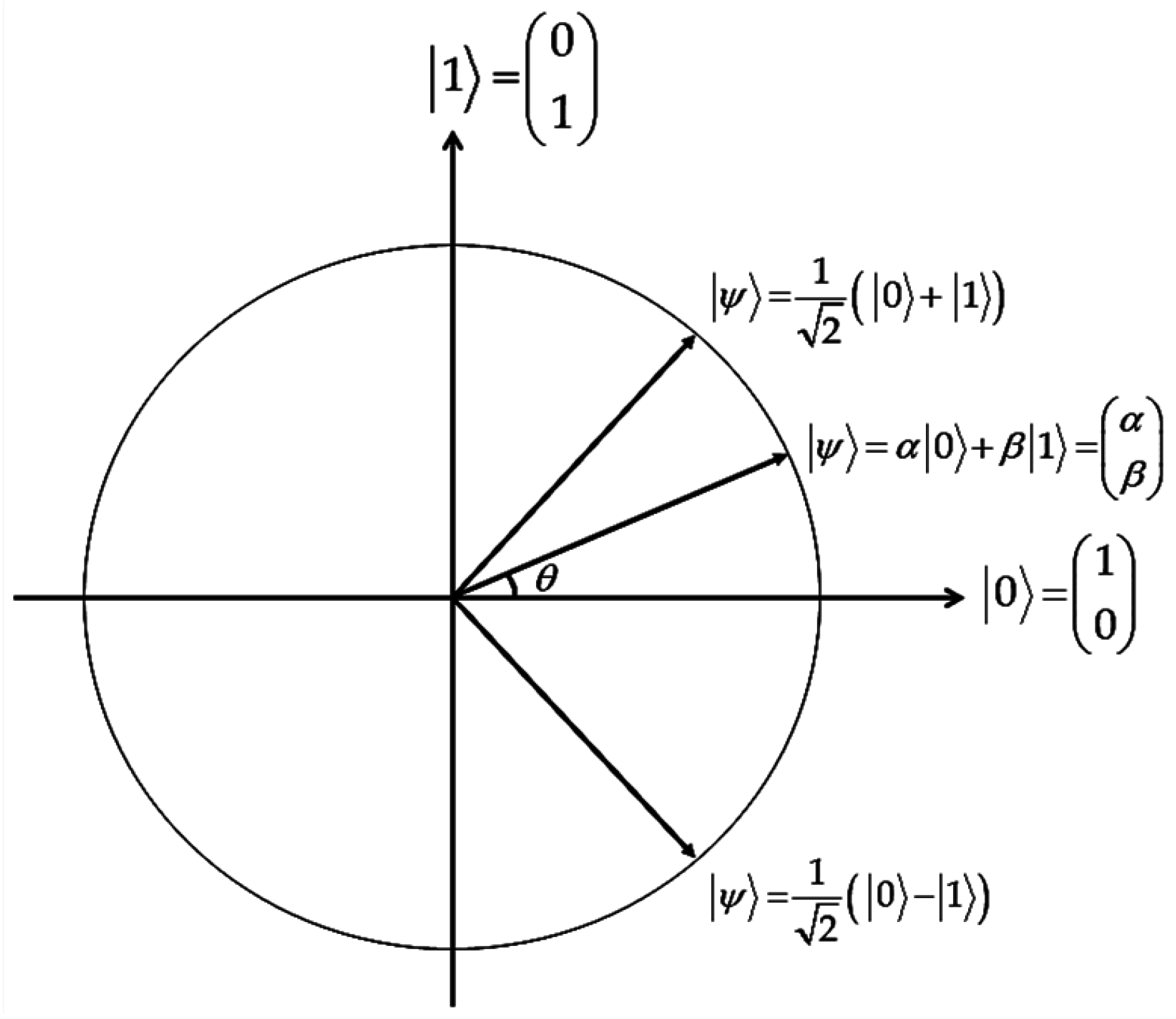
Figure 2.
U-controlled gates. (a) CNOT gate; (b) CCNOT gate.
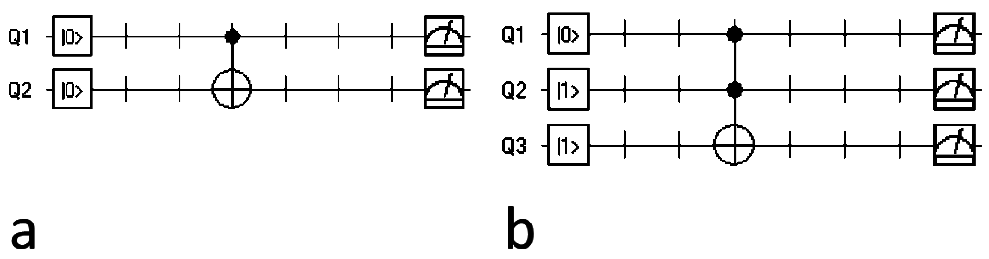
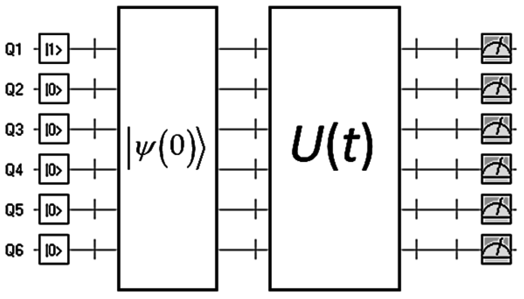
Figure 3.
Quantum circuit including (from left to right) a quantum register, input state , information processing step U(t), and the output as a result of measuring or observing the state of each qubit.
Figure 3.
Quantum circuit including (from left to right) a quantum register, input state , information processing step U(t), and the output as a result of measuring or observing the state of each qubit.

Figure 4.
EPR circuit.
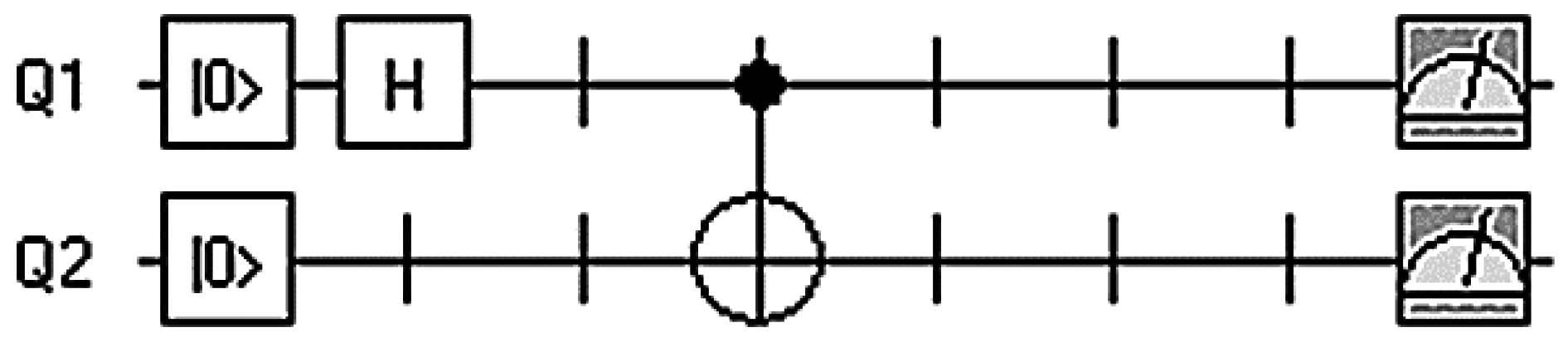
Figure 5.
An example of QCL program (for explanation see text).
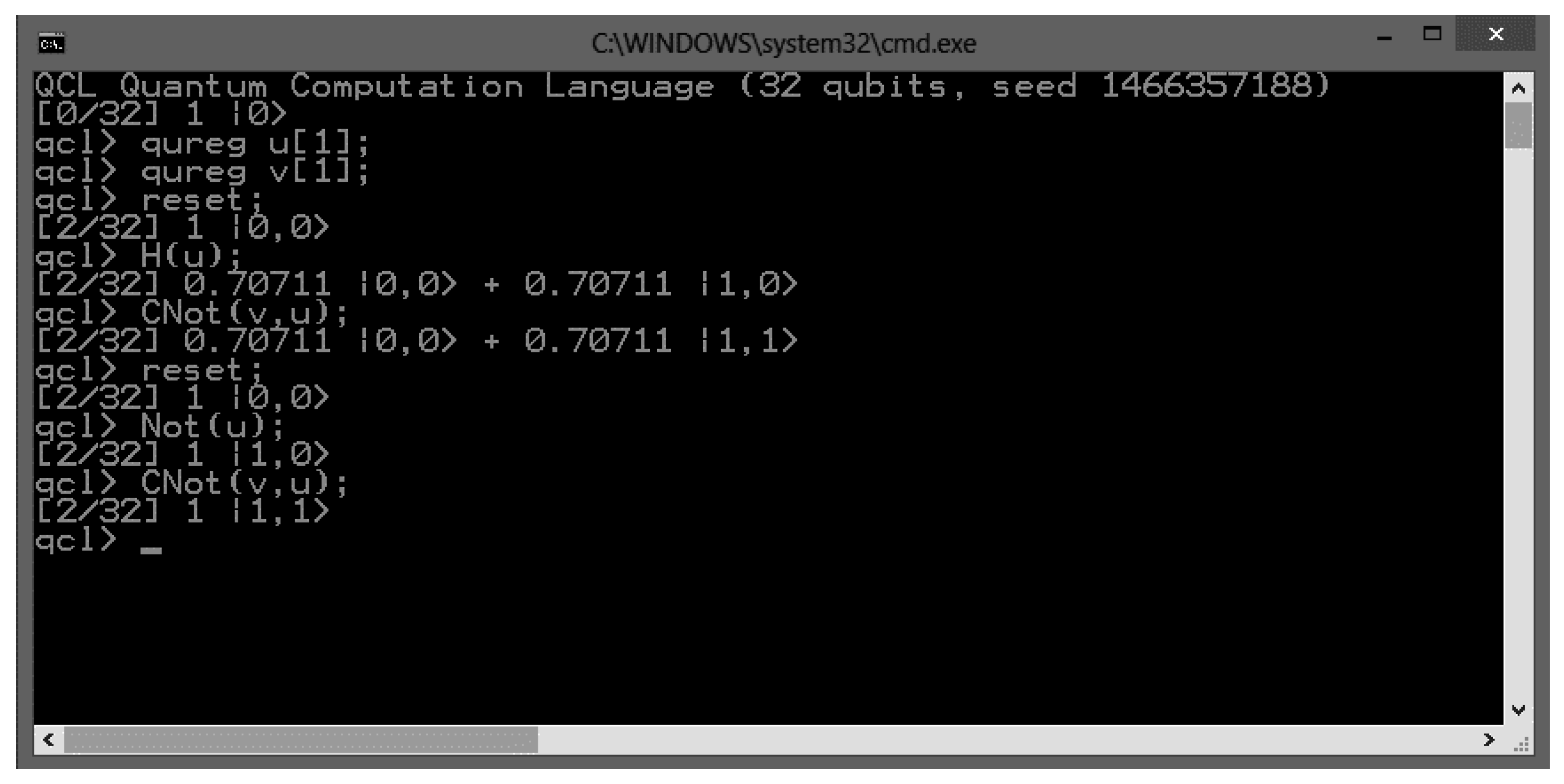
Figure 6.
QRAM architecture (for explanation see text).

Figure 7.
DNA modeled as and gene sequence represented as qubit in a superposition state.

Figure 8.
Rotation gate (for explanation see text).

Figure 9.
Fitness quantum gate.
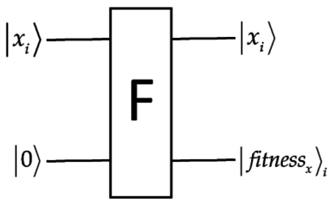
Figure 10.
Quantum circuit representing the RQGA.
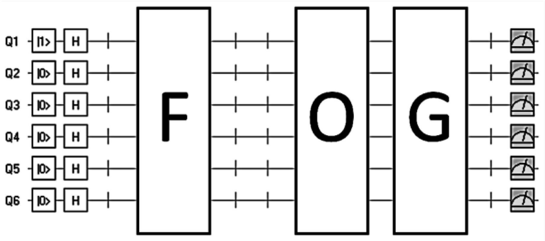
Figure 11.
Representative performance graph obtained in the benchmark function optimization experiments conducted with (a) Quantum genetic algorithm (QGA); (b) Hybrid genetic algorithm (HGA) with mutation; (c) Hybrid genetic algorithm (HGA) without mutation; (d) Simple genetic algorithm (SGA).
Figure 11.
Representative performance graph obtained in the benchmark function optimization experiments conducted with (a) Quantum genetic algorithm (QGA); (b) Hybrid genetic algorithm (HGA) with mutation; (c) Hybrid genetic algorithm (HGA) without mutation; (d) Simple genetic algorithm (SGA).

Figure 12.
Notched Box-and-Whisker Plots, one boxplot per evolutionary algorithm showing the medians (notches) and means (crosses) of the fitness [70]. Squares indicate outliers (unusual fitness values).
Figure 12.
Notched Box-and-Whisker Plots, one boxplot per evolutionary algorithm showing the medians (notches) and means (crosses) of the fitness [70]. Squares indicate outliers (unusual fitness values).

Figure 13.
Performance graph obtained in the benchmark function optimization experiment conducted with RQGA, a true quantum genetic algorithm based on Grover’s algorithm.
Figure 13.
Performance graph obtained in the benchmark function optimization experiment conducted with RQGA, a true quantum genetic algorithm based on Grover’s algorithm.


| Step | |
|---|---|
| 1 | Randomly initialize a population P(0) |
| 2 | Evaluate P(0) |
| 3 | while (not termination condition) do |
| 4 | begin |
| 5 | t ← t + 1 |
| 6 | Selection of parents from population P(t) |
| 7 | Crossover |
| 8 | Mutation |
| 9 | Evaluate P(t) |
| 10 | end |
| Q1 | Q2 | Q1 | * Q2 |
|---|---|---|---|
| 0 | 0 | 0 | 0 |
| 0 | 1 | 0 | 1 |
| 1 | 0 | 1 | 1 |
| 1 | 1 | 1 | 0 |
* Observed after performing the measurement.
| Q1 | Q2 | Q3 | * Q3 |
|---|---|---|---|
| 0 | 0 | 0 | 0 |
| 0 | 0 | 1 | 1 |
| 0 | 1 | 0 | 0 |
| 0 | 1 | 1 | 1 |
| 1 | 0 | 0 | 0 |
| 1 | 0 | 1 | 1 |
| 1 | 1 | 0 | 1 |
| 1 | 1 | 1 | 0 |
* Observed after performing the measurement.
| Step | |
|---|---|
| 1 | Prepare an input state |
| 2 | Apply quantum parallelism |
| 3 | Performs quantum information processing |
| 4 | Use interference to exploit the parallelism |
| 5 | Make a measure |
| Quantum Circuit Example | Symbol | Input → Output * |
|---|---|---|
 |  | |
 |  | |
 |  | |
 |  | |
 |  | |
 |  | |
 |  | |
 |  |
* Output value and probability of being observed after performing the measurement.
| Step | Quantum Computing | Classical Computing |
|---|---|---|
| 1 | Initialize a quantum population Q(0) | |
| 2 | Make P(0), measure of every individual Q(0) → P(0) | |
| 3 | Evaluate P(0) | |
| 4 | while (not termination condition) do | |
| 5 | begin | |
| 6 | t ← t + 1 | |
| 7 | Update Q(t) applying Q-gates: Q(t + 1) = U(t).Q(t) | |
| 8 | Make P(t), measure of every individual Q(t) → P(t) | |
| 9 | Evaluate P(t) | |
| 10 | end |
| 0 0 | False | 0 | - | - | - | - |
| 0 0 | True | 0 | - | - | - | - |
| 0 1 | False | +1 | −1 | 0 | 1 | |
| 0 1 | True | −1 | +1 | 1 | 0 | |
| 1 0 | False | −1 | +1 | 1 | 0 | |
| 1 0 | True | +1 | −1 | 0 | 1 | |
| 1 1 | False | 0 | - | - | - | - |
| 1 1 | True | 0 | - | - | - | - |
| Step | Quantum Computing | Classical Computing |
|---|---|---|
| 1 | Initialize a quantum population Q(0) | |
| 2 | Make P(0), measure of every individual Q(0) P(0) | |
| 3 | Evaluate P(0) | |
| 4 | while (not termination condition) do | |
| 5 | begin | |
| 6 | t t + 1 | |
| 7 | Rotation Q-gate | |
| 8 | Mutation Q-gate | |
| 9 | Make a measure Q(t) P(t) | |
| 10 | Evaluate P(t) | |
| 11 | end |
| Step | Quantum Computing | Classical Computing |
|---|---|---|
| 1 | Initialize a quantum population Q(0) | |
| 2 | Make P(0), measure of every individual Q(0) P(0) | |
| 3 | Evaluate P(0) | |
| 4 | while (not termination condition) do | |
| 5 | begin | |
| 6 | t t + 1 | |
| 7 | Rotation Q-gate | |
| 8 | Crossover operator | |
| 9 | Mutation Q-gate | |
| 10 | Make a measure Q(t) P(t) | |
| 11 | Evaluate P(t) | |
| 12 | end |
| Step | Quantum Computing |
|---|---|
| 1 | Initialize a superposition of all possible chromosomes |
| 2 | Evaluates fitness with operator F |
| 3 | Apply Grover’s algorithm |
| 4 | Ask to the oracle O |
| 5 | Apply Grover’s diffusion operator G |
| 6 | Make a measure |
| Algorithm | Sample Size | Mean Rank |
|---|---|---|
| SGA | 50 | 325.5 |
| HGA1 | 50 | 119.12 |
| HGA2 | 50 | 111.52 |
| HGA3 | 50 | 202.98 |
| QGA1 | 50 | 151.3 |
| QGA2 | 50 | 184.38 |
| QGA3 | 50 | 133.7 |
Statistic = 161.425; p-value = 0.0.
| State | ||
|---|---|---|
© 2016 by the author; licensee MDPI, Basel, Switzerland. This article is an open access article distributed under the terms and conditions of the Creative Commons Attribution (CC-BY) license (http://creativecommons.org/licenses/by/4.0/).
Share and Cite
MDPI and ACS Style
Lahoz-Beltra, R. Quantum Genetic Algorithms for Computer Scientists. Computers 2016, 5, 24. https://doi.org/10.3390/computers5040024
AMA Style
Lahoz-Beltra R. Quantum Genetic Algorithms for Computer Scientists. Computers. 2016; 5(4):24. https://doi.org/10.3390/computers5040024
Chicago/Turabian StyleLahoz-Beltra, Rafael. 2016. "Quantum Genetic Algorithms for Computer Scientists" Computers 5, no. 4: 24. https://doi.org/10.3390/computers5040024
Note that from the first issue of 2016, this journal uses article numbers instead of page numbers. See further details here.