A New Method of Histogram Computation for Efficient Implementation of the HOG Algorithm †


1
Department of Electronics, Telecommunications and IT, University Politehnica Bucharest, Bucharest 060042, Romania
2
Department of Automatics and Computer Science, University Politehnica Bucharest, Bucharest 060042, Romania
*
Author to whom correspondence should be addressed.
†
This paper is an extended version of our paper published in the 9th Computer Science & Electronic Engineering Conference (CEEC), Colchester, UK, 27–29 September 2017.
Computers 2018, 7(1), 18; https://doi.org/10.3390/computers7010018
Submission received: 5 January 2018
/
Revised: 11 February 2018
/
Accepted: 27 February 2018
/
Published: 1 March 2018
(This article belongs to the Special Issue Selected Papers from the 9th Computer Science and Electronic Engineering Conference (CEEC 2017))
Abstract
:In this paper we introduce a new histogram computation method to be used within the histogram of oriented gradients (HOG) algorithm. The new method replaces the arctangent with the slope computation and the classical magnitude allocation based on interpolation with a simpler algorithm. The new method allows a more efficient implementation of HOG in general, and particularly in field-programmable gate arrays (FPGAs), by considerably reducing the area (thus increasing the level of parallelism), while maintaining very close classification accuracy compared to the original algorithm. Thus, the new method is attractive for many applications, including car detection and classification.
1. Introduction
Perception algorithms for intelligent cars have been an important research topic for more than a decade. Significant progress has been achieved [1,2,3,4,5,6] and such algorithms are used for both autonomous car prototypes and for commercial driver assistance systems [4,5,6]. As is known [7,8], a video camera is the preferred sensor (sometimes integrated with a 2D laser [9]) due to its cost. At the same time, the support vector machine (SVM) classifier and the histogram of oriented gradients (HOG) as feature extractor are the most popular solution for object detection and classification [10]. Since HOG is a computationally intensive algorithm, it has been implemented on different platforms, such as graphical processors (GPUs) and more recently on Field-Programmable Gate Arrays (FPGAs). The latter have superior performance in terms of cost, speed, and power consumption [11,12]. All these aspects are essential for commercial applications in general and in particular for enabling classification systems that can work at high vehicle speed.
We believe that optimal implementations of the HOG algorithm can only be achieved if its parameters are properly selected [13] and if the algorithm is modified so that it fully enables an FPGA implementation which has a reduced area, computation time, and power consumption compared with the implementation of the classical HOG. Therefore, our main contribution presented in the paper is a new method for histogram computation which is simpler than the original one and can be implemented using less FPGA resources, thus allowing a higher degree of parallelism and, consequently, a higher speed. We already introduced some algorithm simplifications [14] which we will use in this paper as part of a new histogram computation method. The main challenge for the new method, and for all algorithm modifications in general, is to preserve an overall classification accuracy which is similar to that obtained when the classical HOG is used for feature extraction. We applied the new histogram computation method for car classification, which is an important application area, and less covered than others, but the method can be used for any of the numerous classification applications in which SVM and HOG are employed.
The paper is an extended and reviewed version of [1] and is organized as follows: in Section 2, we present some of the existing literature related to the HOG algorithm, including previous simplifications attempts and previous HOG implementations in FPGAs; in Section 3, we briefly review the classical HOG algorithm and the preliminary simplifications which we will use in the new computation method; in Section 4, we will discuss the new method; and in Section 5, we will present the results of its testing.
2. Related Work
The HOG algorithm was introduced in [15]. The authors performed a thorough analysis of how it can be used to extract image features, for an SVM classifier, for a pedestrian detection application. Their analysis includes the impact of different parameters on the overall classification performance. As we showed in [13], some of their findings can be directly used for any application (this includes, e.g., the number of bins, the type of normalization) while others, such as the cell size, the final descriptor representation, etc., may depend on the application.
Several attempts have been made to reduce the complexity of the classification process, including some proposals for reducing the HOG computation time.
In [16] is shown how the overall prediction time can be decreased, exploiting the fact that for positive (car) images, the HOG, represented in 8 bins, is symmetrical. Because the dimension of the feature vector is reduced to half, this also reduces (a little) the HOG computation time, as well as the classifier time. The authors show a reduction of about 30% of the total computation time, but without detailing the test conditions. In our opinion, the limitation of this method is that it can be applied only to front/rear views of cars, for which image symmetry exists. Also, in our opinion, for large sliding windows (compared to car size), the image and also the HOG are less symmetrical, due to the impact of other objects in the window.
In [17] is discussed another particular approach for faster car detection. It is based on the idea of detecting the shadow region under the cars. Again, it works when the car is seen from the front or rear. A relatively simple threshold technique is applied to identify the shadow regions in the image. An SVM with the HOG approach is then used to classify these regions as being (or not) car shadows. The method seems very interesting, due to the fast processing: the HOG is extracted from relatively few, small regions of the initial image, instead of the entire image. The authors claim a detection rate similar to or slightly better than other methods. However, as limitations, we think that it can be applied only in daytime, it depends on lighting conditions and relative sun position, and it is possible only from the front or rear view.
The literature also contains reports on HOG implementations in FPGAs, especially for pedestrian detection [18,19,20,21,22,23,24,25,26,27,28,29]. For us, it is interesting to note that they also include some previously introduced simplifications of HOG calculation, which are mostly implementation-related simplifications, rather than intrinsic algorithm changes. Such changes include the usage of lookup tables (LUTs) for obtaining the square root, replacement of several multiplications by shifting operations, as well as using for normalization the closest power-of-two number [21,22]. In [18] the authors present in detail the implementation of HOG and SVM, for person detection, on an FPGA. One new aspect presented in the paper is the effect of fixed-point number representation on the system precision. The conclusions are that a fixed-point representation of 18 bits or more introduces no error (compared with the floating-point reference implementation); for 17–12 bits, the introduced error is relatively small (less than 2% absolute error); whereas for 11 bits it goes over 2%. The authors select 13 bits for their final implementation. However, according also to [13], we believe that the number of bits in the fixed-point implementation does not have to be the same for all algorithm steps. Consequently, we believe it is important to evaluate the impact of a different number of bits at each computational stage to select the optimal combination.
In [23,24] the authors propose a very efficient implementation of the HOG and SVM algorithm, for person detection, initially in an FPGA [23], then on an Application Specific Integrated Circuit (ASIC) [24]. Their approach is focused on allowing maximum parallel implementation of the algorithms in hardware. For this, several algorithm simplifications are introduced. Thus, on the HOG side, the histogram extraction on the overlapping blocks is no longer performed. The most interesting proposal seems to be the execution of the SVM after the HOG for each block is calculated, and not at the end, for the entire HOG descriptor. In order to do so, the descriptor for each block is multiplied with the SVM coefficients, and the new result is then accumulated. The authors report a massive improvement in the speed of computation, especially on the SVM side. For the HOG itself, the improvement in speed is about 4 times, compared with a standard implementation with little parallelism. Our simplified method can be applied together with that presented in [23,24]. In fact, according to [24], the histogram calculation in HOG the authors implemented in the FPGA (in [23]) still took around 58% of the entire power consumption of the chip. To resolve the issue of the relatively high power consumption, the authors proceeded to the ASIC implementation [24]. In fact, our simplified HOG algorithm addresses exactly the same issue, decreasing the histogram calculation in HOG.
In [25,26] the authors present another efficient implementation of the same suite of algorithms, still for person detection, using an FPGA, a CPU, and a GPU in a pipeline architecture. In terms of the HOG itself, which is performed on the FPGA, the authors replace the arctangent computation with a suite of multiplications and comparisons. In this way they also avoid computing the division between the two gradient projections. The same approach is used also in [27]. In our approach, one of the simplifications we introduce addresses the same issue of the inefficient arctangent implementation on FPGA, but we compute the gradient slope and instead of a suite of inequalities we have an automatic bin allocation, implemented very effectively by using conventional degrees, so that the couple of multiplications and divisions needed are replaced with shifting operations. The authors do not present a detailed analysis of the speed gained and performance degradation due to this approach, but in [25] they report an overall 6% increase in the miss rate compared with the original algorithm. In our case, we detail these aspects for each of the simplifications we introduced.
In [29] the authors’ focus is, among others, to accelerate the HOG computation by using approximations of the arithmetic operations throughout the algorithm while keeping a limited error at each step. In this way, the final result is comparable with the original one within a controlled error interval and the classification performance is practically identical. By contrast, our goal is to simplify the most time-consuming blocks of the algorithm, thus achieving a superior level of parallelism (and, hence, speed) at the cost of a relatively small performance degradation.
Compared to previous work, which mostly focuses on efficient hardware architectures and also involves some limited HOG algorithm changes, our contribution is the proposal of a new, simpler histogram computation method. This method was conceived so that an optimal FPGA implementation of the HOG feature detector can be achieved. In this paper, we present results obtained for applying it in a car classification system, which is an area less investigated than pedestrian classification. Our results detail the performance of the new method compared with histogram computation in the original HOG.
3. Classical HOG Algorithm and Preliminary Simplifications
Before we present the new histogram computation method, we briefly review the classical HOG algorithm and also some preliminary simplifications we already introduced [14]. This will facilitate understanding of the new method and the reasons why we introduce it. Also, one of the simplifications introduced before, related to the gradient magnitude allocation to the histogram, will be used as a part in the new method.
3.1. Classical HOG Algorithm
As is known [15], the main steps of the algorithm are as follows:
- Computation of x and y gradients for each image pixel;
- Based on the gradients, computation of gradient magnitude and angle (using the arctangent) for each image pixel;
- For each cell of a specified dimension (CellSize), allocate the gradient magnitude in a predefined bin (from a total of NBins) depending on the gradient angle. For example, if NBins = 9, each bin will span over 20 degrees: [0, 20), [20, 40), …, [160, 180]. In general (for all angles which are not exactly in the center of a bin (e.g., 10, 30, etc.)), in the classical approach, the magnitude of the gradients is allocated proportionally to the respective bin and the adjacent one. For instance, a gradient with an angle of 25 degrees, which is closer to the center of Bin 2, will have 75% of its magnitude allocated to Bin 2 and 25% to Bin 1;
- In this way, for each cell is obtained a histogram of oriented gradients, with NBins, and the magnitude of each bin is calculated by adding the interpolated gradient magnitudes of all corresponding pixels;
- Several cells can be grouped together within a block (of BlockSize dimension) and the magnitudes of all histograms are normalized within this block. The normalized values become part of the final algorithm output. All possible combinations of blocks (of given BlockSize) are considered, including overlapping ones.
As can be noticed, the most computationally intensive steps of the algorithm are, particularly for an FPGA implementation, the arctangent, the cell histogram computation, and the block grouping and normalization. In this paper, we address the first two computationally intensive steps.
3.2. Preliminary HOG Simplifications
Before presenting the new histogram computation method, we will briefly review some simplifications we recently proposed [14]. These will be used in the new computation method.
The first simplification involves the bin span representation, and is based on replacing the physical degrees used in the classical algorithm with values which will facilitate the arithmetic operations. We will call these values conventional degrees. Thus, the 0–180° interval used in the classical algorithm for creating the histogram will be replaced by the 0–144 conventional degrees interval. The benefit of this representation is that when using NBins = 9, which was demonstrated by [15] as an optimal choice, the bin span of 20° is replaced by one of 16 conventional degrees. By this change, several multiplications and divisions will be replaced by shifting operations. As discussed in [13], this change does not modify at all the HOG algorithm output and hence does not affect the classification accuracy.
The second simplification, presented also in [14], consists of eliminating the interpolation between bins. For the sake of simplicity we will discuss it using physical degrees but, of course, in the actual implementation it is worth using the conventional degrees mentioned above. According to this simplified approach, a gradient with the angle of, e.g., 22° would be fully assigned to Bin 2 (within the interval 20–40°), instead of interpolating its magnitude between Bin 1 and Bin 2 as in the classical algorithm. As it can be easily seen, this significantly reduces the algorithm complexity, because it removes all the arithmetic and control operations requested by the interpolation. In [14] we demonstrated that, from a theoretical point of view, although the HOG output will be completely different, this change should not necessarily affect the classification algorithm accuracy. Based on the tests performed, we showed that in reality the precision–recall curves are slightly different compared with those of the original algorithm, in some regions being slightly better. Overall, the conclusion is that this simplification maintains a classification accuracy which is very close to that of the original algorithm and, due to its important positive impact on implementation complexity, it should be used in most applications [14].
In this paper, we will use these two simplifications together with a solution for replacing the arctangent computation, thus obtaining a new histogram computation method which we will show to be considerably more efficient to implement than the computation used in the classical HOG.
4. New Histogram Computation Method
As seen in Section 3, the classical histogram computation is based on two steps, both highly computational intensive: first, the angle is computed for each gradient vector (using the arctangent function and the projections of the gradient on x and y axis); then, based on angle, the magnitude of the gradient is allocated to the respective bins. The main bin is the one containing the determined angle of the gradient, but the magnitude is interpolated between this bin and one of its neighbors, depending on the value of the angle compared to the center of the main bin.
Our new histogram computation method replaces both these steps with simpler ones which are much more efficiently implemented in hardware.
4.1. Replacing the Arctangent with Slope
As mentioned above, especially in a hardware implementation, the arctangent computation is one of the blocks requiring many resources, especially in terms of area. On our Artix-7 (XC7A200T-1SBG484C) evaluation board, the Cordic IP used for computing the arctangent uses 386 LUTs and 353 registers and is, in all possible configurations, at least twice the area of a divider.
To overcome this problem, a possible solution is to replace the arctangent computation with an approximate one. As is known, there are several approximations of the arctangent proposed [30]. In general, these approximations still require multiple operations and/or several divisions.
Instead of approximating the arctangent, we propose to replace it with the slope computation. Indeed, the role of the arctangent computation within the original algorithm is to allow the allocation of each gradient within the right bin, based on the gradient angle determined by the arctangent. We propose, instead of the angle, to use the slope of the gradient for this purpose. As is known, the slope can be computed by the ratio y/x, where y and x are the gradient projections on the Cartesian coordinates. These projections are directly obtained when the gradients are computed.
4.1.1. Case of y and x Strictly Positive (Angles in the First Quadrant)
To begin, we will consider the situation when both y and x are strictly positive numbers. There are two important differences between the arctangent and the slope, if we consider them both as functions of (y, x). On one hand, the arctangent is bounded to π/2, whereas the slope is unlimited. On the other hand, for practically every interval, the variation of the slope is much more rapid than the variation of the arctangent.
To deal with the first difference, we can saturate the slope to a certain value. We can select this value to be numerically equal to π/2 (for the sake of consistency with the arctangent output, even if for the arctangent this is measured in radians, whereas for slope it is a nondimensional value).
Therefore, we will define the limited slope (ls) as
However, in this case, the more rapid variation of the slope could lead to a reduced differentiation of values at one of the interval limits. For instance, taking different values for (y, x), we can compare the output of the two functions. The results are shown in Table 1, where we also included the arctangent conversion to degrees and the corresponding conversion of ls(y, x) to the same numerical interval, as well as the main bin containing the respective values. As it can be seen, for all ratios y/x > π/2, the output of the ls function is saturated; hence, all values will be allocated to Bin 5. This is numerically equivalent to considering all angles larger than 57° as being in the same bin. Clearly, this is an important problem, because not being able to differentiate angles larger than 57° is expected to have an important impact on the classifier accuracy.
There are several possibilities to deal with this problem. Our approach (chosen for compatibility reasons) is to keep the saturation at π/2, but decrease the variation of the limited slope (ls) function so that the saturation occurs only for larger values (e.g., for values for which the arctangent values are larger than 80°, which correspond to allocation into the last bin). In this case, the function ls becomes
with parameter k > 1. For the y/x ratios considered above, we can see that a constant k = 4 is acceptable as it maintains an output different than 90° for all angles lower than around 80° and saturates only if the y/x ratio is larger than around 6. Because we consider grey images represented in 8 bits (with each pixel within [0, 255]), when the gradients are computed, they are in the general case in the [−255, 255] interval. However, considering only the positive gradients, they will be within [0, 255]. Because of this, y/x ratios larger than 6 can only happen if x is smaller than approximately 42°. On the other hand, if x is large, using k = 4 will lead to a similar reduced differentiation, but around 0 (in the first bin). Indeed, considering, e.g., x = 70, simple computation shows that all gradients with real angles 0–55° are all put in the same bin because the ls values are very small for all y < 100. Consequently, the value of k has to be changed depending on x. In our implementations we generally considered the following scheme for varying k:
One of the aspects to be investigated is if other values for k lead to better performance and also if they depend on the training/test set.
4.1.2. General Case (Angles in All Four Quadrants)
For angles in the other three quadrants, the arctangent function provides as outputs (after conversion to angles):
- -
- angles within [90°, 180°], if y > 0, x < 0,
- -
- negative angles within [0°, −180°], for y < 0.
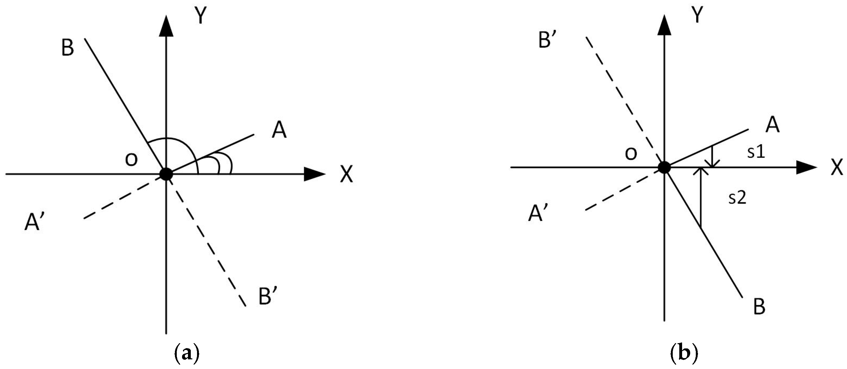
The classical HOG algorithm can work with both signed and unsigned angles. Usually the unsigned representation is preferable, as demonstrated in [14]; hence, the negative angles are converted to positive values by adding 180°. Through this operation, an angle of, e.g., −10° is converted to 170°. This makes perfect sense because the gradients with these two angles are on the same line (which corresponds to an edge in the image) and the descriptor should depend on the lines/edges. Therefore, the output of the arctangent, with this correction, will be in the interval [0°, 180°] when expressed in angles. This is illustrated in Figure 1a, where gradients with negative angles (OA’ and OB’) are represented by gradients on the same line (OA and OB) but with positive angles.
In our case, the ratio y/x depends on the signs of both y and x. Thus, for both y < 0 and x < 0, the output of the limited slope is positive and identical with the output obtained for |y| and |x|. This is acceptable for us because we obtain the same output for gradients on the same line, irrespective of their placement in Quadrant I or III. Similarly, if x × y < 0, the output will be the same for both the case when gradient is in Quadrant II and when in Quadrant IV.
Therefore, the simplest way is to consider the same expression for the limited slope function, irrespective of the signs of y and x. With the corresponding limitations, the function will therefore be
Its output will therefore be in the interval [−π/2, π/2], or, equivalently, within [−90, 90]. This is illustrated in Figure 1b, where gradients with negative x (OA’ and OB’) are represented with gradients on the same line (OA, OB) but with positive x. The slopes of these gradients (s1 and s2) are either positive or negative depending on the sign of the y-axis projection. By adding π/2, we can transform the output interval to one which is similar to that of the classical HOG.
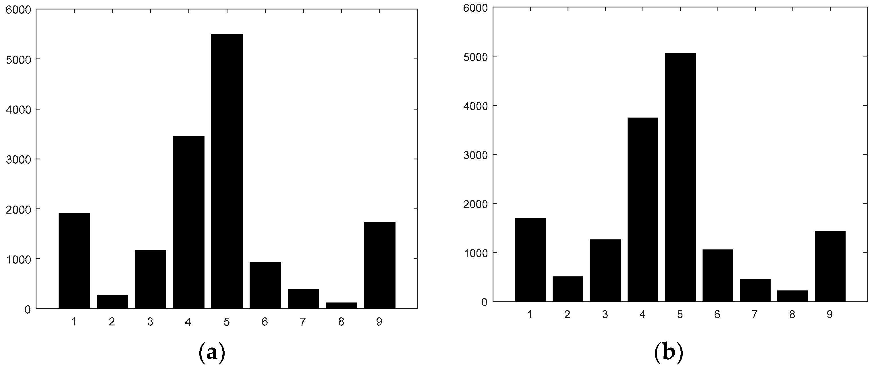
It is important to note that the histogram produced by the new computation method is completely different than that produced by the classical HOG. Indeed, for the same gradients, the slope has in general a value which is completely different than that of the angle; hence, that gradient will be allocated to a different bin than in the case of the classical HOG. Also, the bins of the histograms are within a different interval than for classical HOG ([−90, 90] versus [0°, 180°]). This means that the HOG output will be completely different. However, since this type of output will be used consistently for both training and testing, the classifier will be able to work in a similar manner. The exact performance will be determined by tests. For example, in Figure 2a,b we present cell histograms calculated using the arctangent function and the limited slope function, respectively. In both cases we used the classical allocation approach based on interpolating the magnitude between adjacent bins.
As can be seen, the two histograms look very different. Upon closer inspection, we can see that in the histogram based on arctangent, the most important angles correspond to 90°, 0° (Bins 1 and 9), and angles close to 180°. For the histogram based on slope, we can see that the important bins correspond also to small slopes, close to zero (Bins 5 and 6), and to very large slopes (Bins 1 and 9). However, the magnitude of bins corresponding to small slopes in Figure 2b is larger than that of bins corresponding to low angles in Figure 2a, whereas the magnitude of bins with large slopes is less important in Figure 2b compared with in Figure 2a.
4.2. New HOG Computation Method
By using the slope-based algorithm for determining the histogram bin, and the simplified magnitude allocation with no interpolation (see Section 3.2) a new method for histogram computation is obtained. Additionally, the no-interpolation allocation uses 9 bins of 16 conventional degrees each (see Section 3.2). The new approach is significantly simpler than the one in the original HOG. This is because it replaces the arctangent with a division, eliminating all the divisions and multiplications as well as the control code associated with the magnitude interpolation between adjacent bins, and because it replaces divisions to 20° with shifting.
However, because the new method contains simplified algorithmic blocks compared with the original one, it is important to determine how the classification accuracy is affected. We already showed [14] that the no-interpolation magnitude allocation maintains good classification accuracy when used together with the arctangent function. Since the slope introduced in the new algorithm is significantly different than the angle determined by the arctangent, it is important to study how this affects the magnitude allocation.
5. Results
For tests, we used a combination of static images from several databases as well as from pictures we took in traffic (highway, rural, and in town). These can be found and downloaded at [31]. We created two sets of training and test images. Thus, for Training Set 1 we used a combination of images provided by [32,33] for cars and non-cars, respectively. For Test Set 1 we used pictures from [34]. Training Set 1 consisted of 1700 negative images and 500 positive ones. Test Set 1 consisted of 113 pictures with no cars and 115 pictures with cars. For Training Set 2, we used our own pictures as well as selected pictures from [32]—in total, 848 negative images and 655 positive images. For Test Set 2, we used our own pictures, with 182 negative images and 120 positive images. The training and the test images had the size of 220 × 160 pixels. An example of images from each of the two sets is presented in Figure 3.
In all tests we determined and compared the precision and the recall values, the precision vs recall curves, as well as the area under curve (AUC) for each precision–recall curve. The classifier we used in all tests is a nonlinear SVM with an order 3 polynomial kernel. Within the SVM, the kernel maps the feature n-dimensional space into a space where the values are more easily separable within the two classes (cars and non-cars). Using such a kernel, the classification performance increases compared with that of the linear SVM.
5.1. Tests for Replacing the Arctangent with Slope
We first tested the classical HOG algorithm, replacing only the angle computation (given by the arctangent) with the gradient slope, explained in Section 4. The tests were done on the above data sets and we compared the precision and the recall with those of the standard algorithm using the arctangent.
The results are presented in Table 2 below for different combinations of training and test data. The very low recalls obtained when we combined different sets for training and test (especially in the last case) can be explained by the very different quality of the images in the two sets, as well as by the fact that in Set 2 only front- and rear-view car images are used, whereas Set 1 contains images from all views, including lateral.
As can be seen, the precision is very similar between the two algorithms in most situations. The recall is lower by 1% and 3% (absolute values), respectively, in the first two scenarios. Overall, we can say the performance is not much affected by using the allocation in bins based on gradient slope, instead of using the arctangent.
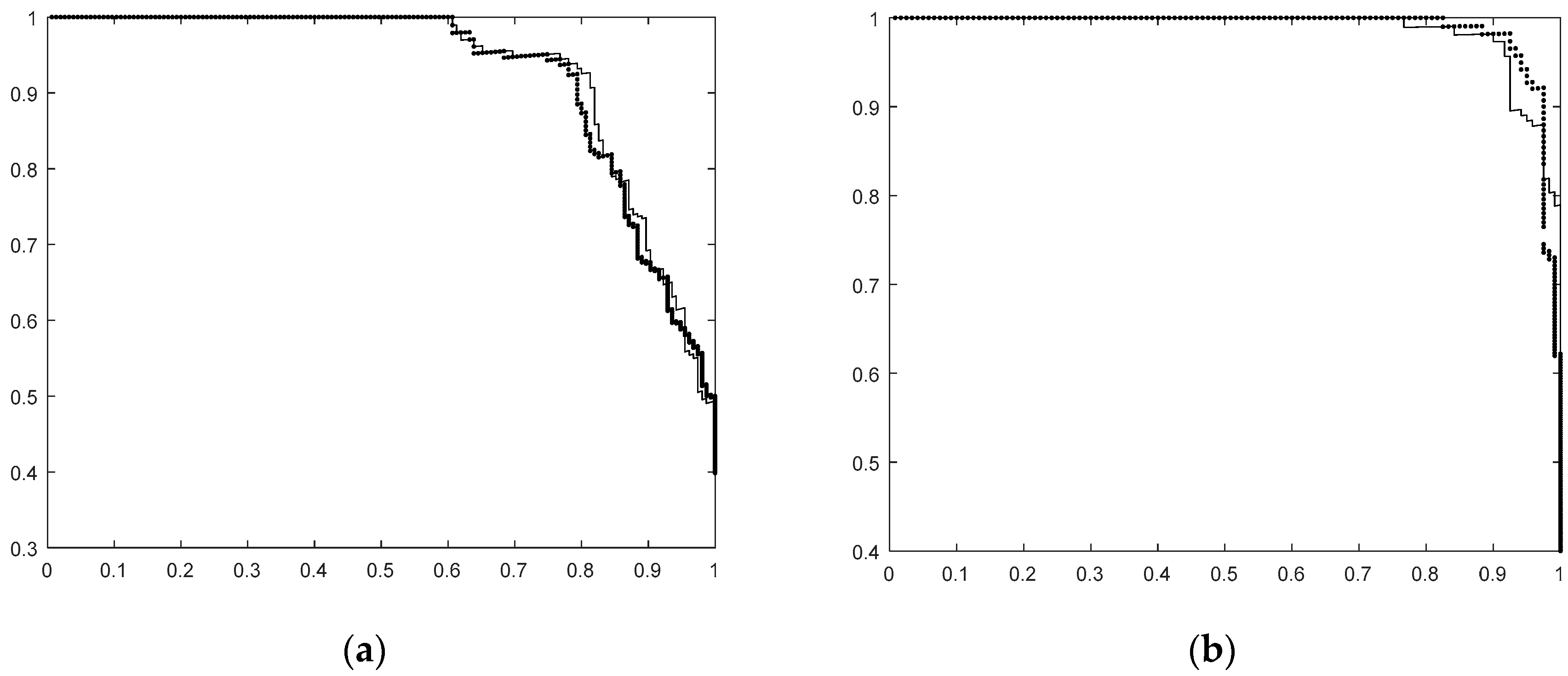
This is confirmed by the precision-recall curves. In Figure 4a,b we show this curves for the first two situations (corresponding to first two lines in Table 2). The precision–recall curves we present are based on the classifier score. As can be seen, the curves are very similar in both situations. For the classifier using the HOG based on gradient slope the curves look, in the region of interest, slightly worse for Set 1 and slightly better for Set 2 compared to that using the original HOG.
In all tests, the k constant was kept at the values defined in Formula (3) (see Section 4). Changing it slightly does not greatly affect the performance, while larger changes decrease the precision and the recall in all situations. Consequently, we can conclude that k as defined in Formula (3) does not depend on the training/test data, which is a positive aspect.
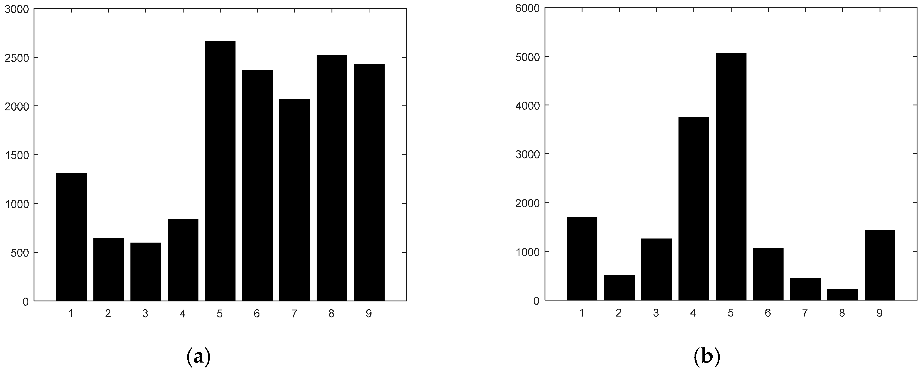
Another aspect which we investigated is how the performance is influenced using the new algorithm if we force all gradient components on axis x and respectively y to zero if they are smaller than a threshold. In other words, we implemented if (abs(grad_x(i)) < thr) grad_x(i) = 0. The idea for this attempt is given by [13], where we showed that if we truncate the final HOG descriptor to just a few bits, the overall performance may increase because the descriptor becomes “sharper”. Practically, by forcing small gradients to zero, we expect to obtain a filtering effect resulting in a sharper cell histogram, which will then translate into a sharper final descriptor. This is because we expect to increase the bins corresponding to either zero (if the y axis gradient is zero) or 90 (if the x axis gradient is zero), and slightly decrease the adjacent bins. For example, the cell histogram presented in Figure 2b changes after performing such an action to the one shown in Figure 5. Indeed, compared with Figure 2b, we can see that Bins 5 (corresponding to zero) and 1 and 9 (corresponding to +/− 90) are larger, whereas Bins 4, 2, and 8 are smaller, so indeed, the histogram became sharper after the filtering action.
We performed the same tests again, but this time including the gradient filtering as described above for the HOG calculation using the gradient slope. We obtained the results presented in Table 3.
As can be seen, the results seem to depend a lot on the test data. For tests using the data in Set 1 (rows 1 and 4), the improvement is very high, the new results being consistently better than those obtained for the original algorithm (see Table 2, on the same rows). However, when using test data in Set 2 the results are either similar or worse. Consequently, the impact of gradient filtering needs to be further studied, but it seems that for normal operating conditions (when the pictures in the training and the test sets are similar, as in the first two rows in Table 3) gradient filtering may be worth performing.
5.2. Tests for the New HOG Computation Method
In the following step, we tested the new HOG computation method which consists (see Section 4.2) of the slope computation and the no-interpolation gradient magnitude allocation.
We tested the new method in the same conditions as those presented above. Practically, compared to the tests above, we replaced the classical magnitude interpolation between adjacent bins with the simple algorithm presented in Section 3.2 which allocates the entire gradient magnitude to the bin determined based on the slope (without splitting the magnitude with one of the neighbor bins depending on the exact value of the slope). The results are presented in Table 4 (no filtering applied) and Table 5 (filtering with threshold 10 applied to the new method). As can be seen, the results in Table 4 are very close to the results presented in Table 2. This confirms that the simplified magnitude allocation algorithm introduces practically no errors and also shows that the new method, consisting of the bin calculation based on slope and the simplified magnitude allocation algorithm, can be successfully used in FPGA implementations. When filtering is performed, the results are also relatively close to those obtained by the original algorithm (but a little worse compared to Table 3, last two columns). This shows that filtering effect depends even more strongly on the test data when using the no-interpolation magnitude allocation, compared with the case when the original interpolation-based allocation is used. The decision on using (or not) filtering should be made after validating it in real test conditions. Further investigations may be needed to better explain the conditions which need to be satisfied in order for the filtering to improve the classification accuracy.
We used an Artix-7 (XC7A200T-1SBG484C) evaluation board with 33,650 logic slices, each with 4 LUTs and 8 registers, 13 Mbits of RAM, and 740 DSP slices. The implementation was performed using the SystemVerilog language and Vivado Web-Pack tools. In Table 6 we present the areas occupied for the HOG algorithm using each of the preliminary simplifications as well as the full new method for histogram computation. The areas are expressed for both slice LUTs and slice registers in terms of absolute and percentage of the area of the original HOG algorithm implementation.
As can be seen, the area of the HOG using the slope computation (instead of the arctangent) is significantly reduced compared with the area of the original HOG, especially in terms of LUTs. When we also introduce the simplified allocation, the area for the new histogram computation method is further reduced, especially in the slice registers. The reduction due to slope is due not only to the arctangent replacement, but also to the simplification of the logic for the sign correction mechanism.
Since our FPGA has 134,600 LUTs and 269,200 registers, the data in Table 6 show that one can implement three original HOG blocks in parallel, while for the new histogram computation, the parallelism increases to 11. Consequently, the speed increases also by 3.67 times.
In terms of classification accuracy variation, we present in Table 7 the percentage of the recall deterioration compared to the original algorithm (the precision is very little affected by all simplifications).
As can be seen, the decrease in the recall for the new histogram computation is always less than or equal to 3%. As shown in Table 4, the recall deterioration can be as little as 1% depending on the quality of training and test data sets and the number of different angles of car views. We believe that due to the very large reduction of area, the new method will have many applications.
5.3. Tests for Different Classifiers
All tests presented above have been done using an SVM classifier with an order 3 polynomial kernel. In order to see how the classification performance varies with different kernels, for the original as well as the modified computation method we performed the same tests as above, changing the kernel. We considered polynomial kernels of different orders, radial basis function RBF (Gaussian) kernel, and a linear kernel. In all cases, the performance for both computation methods changed similarly so that the difference in performance remained in general in the same interval as that presented in Table 7. The performance increased a little for higher polynomial orders and decreased for all other kernels. An interesting case is when the linear kernel is used. This reduces the complexity of the classifier not only for training but also for testing; therefore, it is worth investigating.
6. Discussions
In this paper we investigated how histogram computation can be made more efficient, especially when implemented within an FPGA. For this, we first showed how the arctangent can be replaced by the computation of a gradient slope. This requires one division in practice and occupies a smaller area than the arctangent. The classification accuracy is very minorly affected by this change. Furthermore, if gradient filtering is introduced, the performance is improved in some situations. These situations depend on the testing data and do not depend on the training ones.
Then, we also replaced the classical interpolation-based magnitude allocation with a simplified one with no interpolation. In this way, a new histogram computation method is obtained. Compared with the original method, it is significantly simpler because it replaces the arctangent with the slope computation and because it eliminates all the divisions and multiplications as well as the control code associated with the magnitude interpolation between adjacent bins. Its significantly smaller area allows a higher level of parallelism and a lower total cost. The no-interpolation mechanism does not introduce significant errors, so the overall accuracy of the new method is very close to that of the original one.
Finally, we tested both methods for different kernels of the SVM classifier. We found that for both methods, the polynomial kernel leads to best performance and, in general, the higher the order of the polynomial, the higher the performance; however, for orders above 3 the improvement is not important. For the linear classifier, which is the simplest, the decrease in performance is significant for both methods.
7. Conclusions
The new method for histogram computation introduced and validated in this paper is significantly less complex than the one in the original HOG. Because of this, it can be implemented in a much smaller area in FPGAs (around 4 times smaller), thus allowing a significant increase in parallelism, and, hence, in speed. The accuracy of the new method is only minorly decreased (less than 3% in absolute value) compared with that of the original one, showing that it can be successfully used in most FPGA-based HOG implementations. Because of the important reduction in speed, it may be also used as a block in more complex descriptors which include HOG plus extra information, such as [22]. The resulting system will have reduced computation time compared to [22], but also a higher accuracy than our current implementation.
Acknowledgments
This work has been partially funded by University “Politehnica” of Bucharest, through the “Excellence Research Grants” Program, UPB–GEX. Project title “The optimization and real-time implementation of artificial intelligence algorithms used in autonomous car applications, to classify moving objects”, Contract 104/26.09.2016 (EL.07.16.13).
Author Contributions
M.-E.I. developed the new slope-based allocation algorithm, the new histogram computation method, performed the algorithms simulations as well as the FPGA implementation and FPGA area calculations. C.I. added a more detailed explanation of the slope-based allocation algorithm, included the area under curve (AUC) criteria for precision-recall comparison, performed the algorithm tests for different classifiers and extended the related work paragraph, covering several other papers.
Conflicts of Interest
The authors declare no conflicts of interest.
References
- Ilas, M.E. New Histogram Computation Adapted for FPGA Implementation of HOG Algorithm—For Car Detection Applications. In Proceedings of the 9th Computer Science & Electronic Engineering Conference (CEEC), Colchester, UK, 27–29 September 2017. [Google Scholar]
- Luettel, T.; Himmelshach, M.; Wuensche, H.-J. Autonomous Ground Vehicles—Concepts and a path to the future. Proc. IEEE 2012, 1831–1839. [Google Scholar] [CrossRef]
- Lozano-Perez, T. Autonomous Robot Vehicles; Cox, I.J., Wilfong, G.T., Eds.; Springer Science & Business Media: Berlin, Germany, 2012. [Google Scholar]
- Rouff, C.; Hinchey, M. Experience from the DARPA Urban Challenge; Springer: London, UK, 2012; ISBN 978-0-85729771-6. [Google Scholar]
- Frazzoli, E.; Munther, D.A.; Feron, E. Real-time motion planning for agile autonomous vehicles. J. Guid. Control Dyn. 2012, 25, 116–129. [Google Scholar] [CrossRef]
- Ilas, C. Electronic sensing technologies for autonomous ground vehicles: A review. In Proceedings of the 8th International Symposium on Advanced Topics in Electrical Engineering (ATEE), Bucharest, Romania, 23–25 May 2013; pp. 1–6. [Google Scholar]
- Ilas, C. Perception in Autonomous Ground Vehicles—A Review. In Proceedings of the ECAI Conference, Pitesti, Romania, 27–29 June 2013; pp. 1–6. [Google Scholar]
- Ilas, C.; Mocanu, I.; Ilas, M. Advances in Environment Sensing and Perception Technologies and Algorithms for Autonomous Ground Vehicles. In Autonomous Vehicles; Bizon, N., Dascalescu, L., Tabatabaei, N.M., Eds.; Nova Science Inc.: New York, NY, USA, 2014; Chapter 4; pp. 113–146. ISBN 971-1-63321-326-5. [Google Scholar]
- Lin, B.Z.; Chien-Chou, L. Pedestrian detection by fusing 3D points and color images. In Proceedings of the IEEE/ACIS 15th International Conference on Computer and Information Science (ICIS), Okayama, Japan, 26–29 June 2016; pp. 1–5. [Google Scholar]
- Sivaraman, S.; Trivedi, M.M. Looking at vehicles on the road: A survey of vision-based vehicle detection, tracking, and behavior analysis. IEEE Trans. Intell. Transp. Syst. 2013, 14, 1773–1795. [Google Scholar] [CrossRef]
- Ma, X.; Walid Najjar, A.; Roy-Chowdhury, A.K. Evaluation and acceleration of high-throughput fixed-point object detection on FPGAs. IEEE Trans. Circ. Syst. Video Technol. 2015, 25, 1051–1062. [Google Scholar]
- Tasson, D.; Montagnini, A.; Marzotto, R.; Farenzena, M.; Cristani, M. FPGA-based pedestrian detection under strong distortions. In Proceedings of the IEEE Conference on Computer Vision and Pattern Recognition Workshops (CVPRW), Boston, MA, USA, 7–12 June 2015; pp. 65–70. [Google Scholar]
- Ilas, M.E. Parameter Selection for Efficient HOG-based car detection. In Proceedings of the IEEE 26th International Symposium on Industrial Electronics (ISIE), Edinburgh, UK, 19–21 June 2017. [Google Scholar]
- Ilas, M.E. HOG Algorithm Simplification and Its Impact on FPGA Implementation—With Applications in Car Detection. Proceedings of 9th IEEE Conference on Electronics, Computers and Artificial Intelligence, Targoviste, Romania, 29 June–1 July 2017. [Google Scholar]
- Dalal, N.; Triggs, B. Histograms of oriented gradients for human detection. In Proceedings of the IEEE Computer Society Conference on Computer Vision and Pattern Recognition, San Diego, CA, USA, 20–25 June 2005; Volume 1. [Google Scholar]
- Lee, SH.; Bang, K.H.; Jung, K. An efficient selection of HOG feature for SVM classification of vehicle. In Proceedings of the IEEE International Symposium on Consumer Electronics (ISCE), Madrid, Spain, 24–26 June 2015; pp. 1–2. [Google Scholar]
- Li, X.; Guo, X. A HOG feature and SVM based method for forward vehicle detection with single camera. In Proceedings of the 5th International Conference on Intelligent Human-Machine Systems and Cybernetics (IHMSC), Hangzhou, China, 26–27 August 2013; Volume 1, pp. 263–266. [Google Scholar]
- Hsiao, P.Y.; Lin, S.Y.; Huang, S.S. An FPGA based human detection system with embedded platform. Microelectron. Eng. 2015, 138, 42–46. [Google Scholar] [CrossRef]
- Benenson, R.; Mathias, C.; Timofte, R.; Van Gool, L. Pedestrian detection at 100 frames per second. In Proceedings of the IEEE Conference on Computer Vision and Pattern Recognition (CVPR), Providence, RI, USA, 16–21 June 2012; pp. 2903–2910. [Google Scholar]
- Hsiao, P.Y.; Lin, S.Y.; Chen, C.Y. A Real-Time FPGA Based Human Detector. In Proceedings of the International Symposium on Computer, Consumer and Control (IS3C), Xi’an, China, 4–6 July 2016; pp. 1014–1017. [Google Scholar]
- Hemmati, M.; Biglari-Abhari, M.; Berber, S.; Niar, S. HOG feature extractor hardware accelerator for real-time pedestrian detection. In Proceedings of the 17th Euromicro Conference on Digital System Design (DSD), Verona, Italy, 27–29 August 2014; pp. 543–550. [Google Scholar]
- Kim, J.; Baek, J.; Kim, E. A Novel On-Road Vehicle Detection Method Using π-HOG. IEEE Trans. Intell. Transp. Syst. 2015, 16, 3414–3429. [Google Scholar] [CrossRef]
- Mizuno, K.; Terachi, Y.; Takagi, K.; Izumi, S.; Kawaguchi, H.; Yoshimoto, M. Architectural study of HOG feature extraction processor for real-time object detection. In Proceedings of the 2012 IEEE Workshop on Signal Processing Systems (SiPS), Quebec City, QC, Canada, 17–19 October 2012; pp. 197–202. [Google Scholar]
- Mizuno, K.; Terachi, Y.; Takagi, K.; Izumi, S.; Kawaguchi, H.; Yoshimoto, M. A sub-100 mw dual-core HOG accelerator VLSI for parallel feature extraction processing for HDTV resolution video. IEICE Trans. Electron. 2013, 96, 433–443. [Google Scholar] [CrossRef]
- Bauer, S.; Köhler, S.; Doll, K.; Brunsmann, U. FPGA-GPU architecture for kernel SVM pedestrian detection. In Proceedings of the 2010 IEEE Computer Society Conference on Computer Vision and Pattern Recognition Workshops (CVPRW), San Francisco, CA, USA, 13–18 June 2010; pp. 61–68. [Google Scholar]
- Bauer, S.; Brunsmann, U.; Schlotterbeck-Macht, S. FPGA implementation of a HOG-based pedestrian recognition system. In Proceedings of the MPC-Workshop, Karlsruhe, Germany, 6 May 2009; pp. 49–58. [Google Scholar]
- Hahnle, M.; Saxen, F.; Hisung, M.; Brunsmann, U.; Doll, K. FPGA-based real-time pedestrian detection on high-resolution images. In Proceedings of the IEEE Conference on Computer Vision and Pattern Recognition Workshops (CVPRW), Portland, OR, USA, 23–28 June 2013; pp. 629–635. [Google Scholar]
- Chen, P.Y.; Huang, C.C.; Lien, C.Y.; Tsai, Y.H. An efficient hardware implementation of HOG feature extraction for human detection. IEEE Trans. Intell. Transp. Syst. 2014, 15, 656–662. [Google Scholar] [CrossRef]
- Wang, J.F.; Choy, C.S.; Chao, T.L.; Kit, K.C.; Pun, K.P.; Ouyang, W.L.; Wang, X.G. HOG arithmetic for speedy hardware realization. In Proceedings of the 2014 IEEE Asia Pacific Conference on Circuits and Systems (APCCAS), Ishigaki, Japan, 17–20 November 2014; pp. 61–64. [Google Scholar]
- Rajan, S.; Wang, S.; Inkol, R.; Joyal, A. Efficient approximations for the arctangent function. IEEE Signal Process. Mag. 2006, 23, 108–111. [Google Scholar] [CrossRef]
- Static Images. Available online: https://drive.google.com/drive/folders/0B7EEW4NFU3YdTUpsRXBNSm1JNEE?usp=sharing (accessed on 28 February 2018).
- Krause, J.; Stark, M.; Deng, J.; Li, F. 3D object representations for fine-grained categorization. Proceedings of IEEE International Conference on Computer Vision Workshops, Sydney, Australia, 2–8 December 2013; pp. 554–561. [Google Scholar]
- Opelt, A.; Pinz, A.; Fussenegger, M.; Auer, P. Generic object recognition with boosting. IEEE Trans. Pattern Anal. Mach. Intell. 2006, 28, 416–431. [Google Scholar] [CrossRef] [PubMed]
- Carbonetto, P.; Dorkó, G.; Schmid, C.; Kück, H.; De Freitas, N. Learning to recognize objects with little supervision. Int. J. Comp. Vis. 2008, 77, 219–237. [Google Scholar] [CrossRef]
Figure 1.
Gradient conversion to two quadrants: (a) classical histogram of oriented gradients (HOG) approach: gradients OA’ and OB’ are converted to OA and OB, respectively, and represented by the angles which are in the 0–180° interval; (b) new computation method: gradients OA’ and OB’ are converted to OA and OB, respectively, and represented by the slopes s1 and s2 which are in the [−90, 90] interval.

Figure 2.
Histogram of gradients: (a) Computed using the arctangent function. Each bin has a 20° span. Bin 1 starts with 0°. Bin 5 contains angles within [80°, 100°]. (b) Computed using the limited slope function. Each bin has a span of 20. Bin 1 starts with −90. Bin 5 contains slopes around 0.
Figure 2.
Histogram of gradients: (a) Computed using the arctangent function. Each bin has a 20° span. Bin 1 starts with 0°. Bin 5 contains angles within [80°, 100°]. (b) Computed using the limited slope function. Each bin has a span of 20. Bin 1 starts with −90. Bin 5 contains slopes around 0.

Figure 3.
Example of images used for training in Set 1 (a) and Set 2 (b).
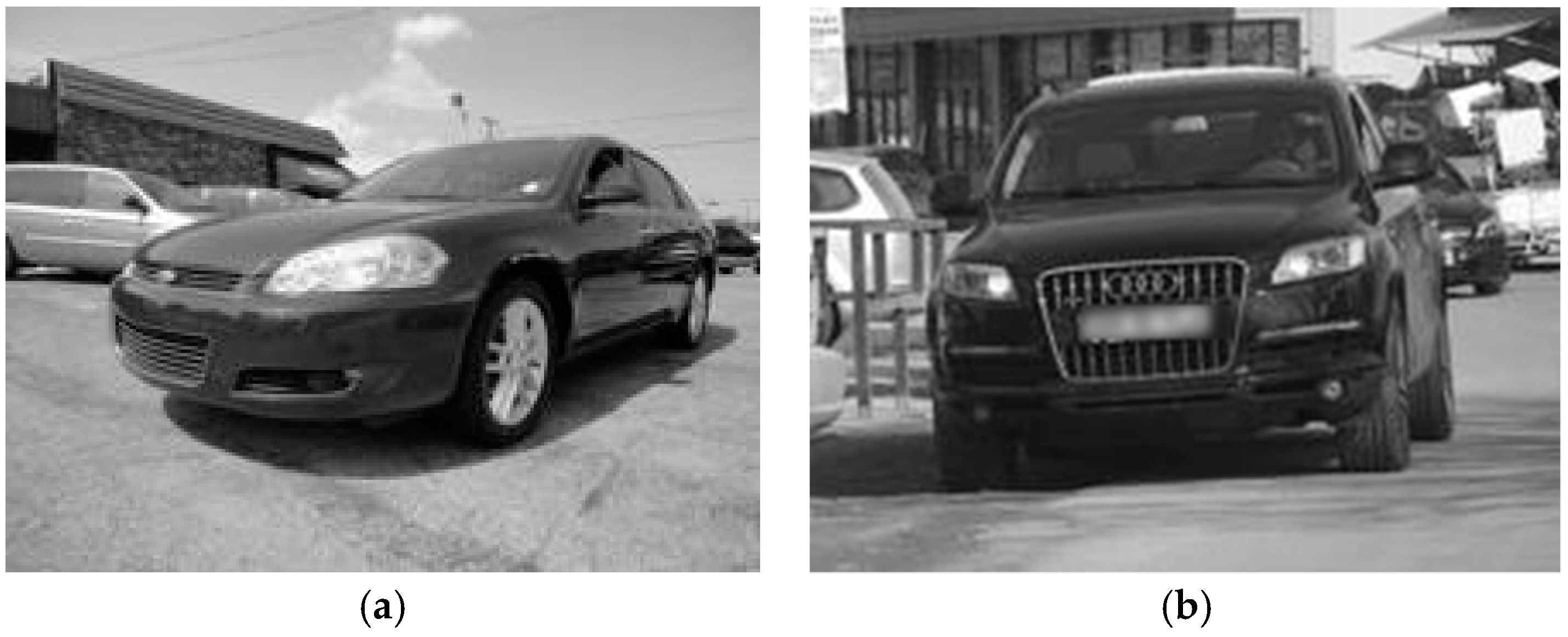
Figure 4.
Precision–recall curves for car classification using the original HOG (solid line, thinner) and the HOG using gradient slope for bin allocation (dotted line, thicker) (a) for Training Set 1, Test Set 1; (b) for Training Set 2, Test Set 2.
Figure 4.
Precision–recall curves for car classification using the original HOG (solid line, thinner) and the HOG using gradient slope for bin allocation (dotted line, thicker) (a) for Training Set 1, Test Set 1; (b) for Training Set 2, Test Set 2.

Figure 5.
Histogram of gradients computed using the limited slope function, for the same cell as the one presented in Figure 2, but after applying the filtering of gradient components, with a threshold of 10 (a). In (b) the original histogram shown in Figure 2b is repeated here, to facilitate comparison.

Table 1.
Different slope values and the corresponding values of arctangent and ls function, together with the resulting allocation bins.
Table 1.
Different slope values and the corresponding values of arctangent and ls function, together with the resulting allocation bins.
| y/x Ratio [-] | Atan(y, x) [rad] | ls(y, x) [-] | Atan(y, x) [deg] | ls × 180/π [-] | Atan Bin | ls Bin |
|---|---|---|---|---|---|---|
| 0.33 | 0.32 | 0.33 | 18.43 | 19.09 | 1 | 1 |
| 0.5 | 0.46 | 0.5 | 26.56 | 28.64 | 2 | 2 |
| 1 | 0.78 | 1 | 45 | 57.3 | 3 | 3 |
| 1.57 | 1.00 | 1.57 | 57.52 | 90 | 3 | 5 |
| 2 | 1.1 | 1.57 | 63.43 | 90 | 4 | 5 |
| 3 | 1.25 | 1.57 | 71.56 | 90 | 4 | 5 |
| 4 | 1.32 | 1.57 | 75.96 | 90 | 4 | 5 |
| 7 | 1.43 | 1.57 | 81.86 | 90 | 5 | 5 |
| 10 | 1.47 | 1.57 | 84.28 | 90 | 5 | 5 |
Table 2.
Precision and recall values for classification using the original HOG and the algorithm using gradient slope for bin allocation.
Table 2.
Precision and recall values for classification using the original HOG and the algorithm using gradient slope for bin allocation.
| Data Sets | Original HOG (Arctangent Based) | New Algorithm (Slope Based) | |||||
|---|---|---|---|---|---|---|---|
| Training | Test | Precision | Recall | AUC | Precision | Recall | AUC |
| Set 1 | Set 1 | 0.99 | 0.65 | 0.927 | 0.98 | 0.62 | 0.921 |
| Set 2 | Set 2 | 0.99 | 0.84 | 0.982 | 0.99 | 0.83 | 0.980 |
| Set 1 | Set 2 | 1 | 0.68 | 0.968 | 1 | 0.70 | 0.969 |
| Set 2 | Set 1 | 0.91 | 0.33 | 0.795 | 0.92 | 0.32 | 0.832 |
Table 3.
Precision and recall values for classification using the algorithm using gradient slope for bin allocation, with and without gradient filtering.
Table 3.
Precision and recall values for classification using the algorithm using gradient slope for bin allocation, with and without gradient filtering.
| Data Sets | New Algorithm (Slope Based, No Filtering) | New Algorithm (Slope Based, with Filtering) | |||||
|---|---|---|---|---|---|---|---|
| Training | Test | Precision | Recall | AUC | Precision | Recall | AUC |
| Set 1 | Set 1 | 0.98 | 0.62 | 0.921 | 1 | 0.69 | 0.919 |
| Set 2 | Set 2 | 0.99 | 0.83 | 0.980 | 1 | 0.83 | 0.972 |
| Set 1 | Set 2 | 1 | 0.70 | 0.969 | 1 | 0.65 | 0.949 |
| Set 2 | Set 1 | 0.92 | 0.32 | 0.832 | 0.97 | 0.42 | 0.881 |
Table 4.
Precision and recall values for classification using the original and the new HOG computation method.
Table 4.
Precision and recall values for classification using the original and the new HOG computation method.
| Data Sets | Original Histogram Computation Method | New Histogram Computation Method | |||||
|---|---|---|---|---|---|---|---|
| Training | Test | Precision | Recall | AUC | Precision | Recall | AUC |
| Set 1 | Set 1 | 0.99 | 0.65 | 0.927 | 0.98 | 0.62 | 0.922 |
| Set 2 | Set 2 | 0.99 | 0.84 | 0.982 | 0.99 | 0.83 | 0.980 |
| Set 1 | Set 2 | 1 | 0.68 | 0.969 | 1 | 0.68 | 0.966 |
| Set 2 | Set 1 | 0.91 | 0.33 | 0.795 | 0.93 | 0.33 | 0.833 |
Table 5.
Precision and recall values for classification using the original and the new HOG computation method, with filtering.
Table 5.
Precision and recall values for classification using the original and the new HOG computation method, with filtering.
| Data Sets | Original Histogram Computation Method | New Histogram Computation Method, with Filtering | |||||
|---|---|---|---|---|---|---|---|
| Training | Test | Precision | Recall | AUC | Precision | Recall | AUC |
| Set 1 | Set 1 | 0.99 | 0.65 | 0.927 | 1 | 0.69 | 0.919 |
| Set 2 | Set 2 | 0.99 | 0.84 | 0.982 | 1 | 0.81 | 0.972 |
| Set 1 | Set 2 | 1 | 0.68 | 0.969 | 1 | 0.63 | 0.949 |
| Set 2 | Set 1 | 0.91 | 0.33 | 0.795 | 0.97 | 0.42 | 0.881 |
Table 6.
Absolute and relative number of slice lookup tables (LUTs) and registers for the simplified versions of HOG, versus the original one.
Table 6.
Absolute and relative number of slice lookup tables (LUTs) and registers for the simplified versions of HOG, versus the original one.
| Implemented Algorithm | Slice LUTs Abs. Value | Slice LUTs Relative Value | Slice Registers Abs. Value | Slice Registers Relative Value |
|---|---|---|---|---|
| Original HOG (with arctangent, bin interpolation, and 20 degree bins) | 42,917 | 100% | 27,808 | 100% |
| HOG with 16 degree bins (with arctangent, bin interpolation, and 16 degree bins) | 40,239 | 93.76% | 23,052 | 82.90% |
| Simplified HOG (with arctangent, no bin interpolation, 16 degree bins) | 15,150 | 35.30% | 17,002 | 61.14% |
| New histogram computation, with slope, no interpolation, and bins of 16 units | 11,075 | 25.81% | 10,928 | 39.30% |
Table 7.
Relative number of slice LUTs and registers for the simplified versions of HOG, versus the original one.
Table 7.
Relative number of slice LUTs and registers for the simplified versions of HOG, versus the original one.
| Implemented Algorithm | Slice LUTs |
|---|---|
| Original HOG (with arctangent, bin interpolation, and 20 degree bins) | - |
| HOG with 16 degree bins (with arctangent, bin interpolation, and 16 degree bins) | 0% |
| Simplified HOG (with arctangent, no bin interpolation, 16 degree bins) | −1 to +1% 1 |
| New histogram computation, with slope, no interpolation, and bins of 16 units | −3 to −1% |
| New histogram computation, with slope, no interpolation, and bins of 16 units, with filtering, on similar training and test data | −3 to +4% 1 |
1 Recall may actually be increased.
Table 8.
Precision and recall values for classification using the original and the new HOG computation method, using a linear SVM classifier.
Table 8.
Precision and recall values for classification using the original and the new HOG computation method, using a linear SVM classifier.
| Data Sets | Original Histogram Computation Method | New Histogram Computation Method | |||||
|---|---|---|---|---|---|---|---|
| Training | Test | Precision | Recall | AUC | Precision | Recall | AUC |
| Set 1 | Set 1 | 0.95 | 0.68 | 0.889 | 0.97 | 0.64 | 0.898 |
| Set 2 | Set 2 | 0.97 | 0.81 | 0.950 | 0.95 | 0.81 | 0.940 |
| Set 1 | Set 2 | 1 | 0.51 | 0.870 | 0.97 | 0.52 | 0.880 |
| Set 2 | Set 1 | 0.89 | 0.30 | 0.741 | 0.92 | 0.36 | 0.800 |
© 2018 by the authors. Licensee MDPI, Basel, Switzerland. This article is an open access article distributed under the terms and conditions of the Creative Commons Attribution (CC BY) license (http://creativecommons.org/licenses/by/4.0/).
Share and Cite
MDPI and ACS Style
Ilas, M.-E.; Ilas, C. A New Method of Histogram Computation for Efficient Implementation of the HOG Algorithm. Computers 2018, 7, 18. https://doi.org/10.3390/computers7010018
AMA Style
Ilas M-E, Ilas C. A New Method of Histogram Computation for Efficient Implementation of the HOG Algorithm. Computers. 2018; 7(1):18. https://doi.org/10.3390/computers7010018
Chicago/Turabian StyleIlas, Mariana-Eugenia, and Constantin Ilas. 2018. "A New Method of Histogram Computation for Efficient Implementation of the HOG Algorithm" Computers 7, no. 1: 18. https://doi.org/10.3390/computers7010018
Note that from the first issue of 2016, this journal uses article numbers instead of page numbers. See further details here.