Performance Evaluation of Discrete Event Systems with GPenSIM


1
Faculty of Science and Technology, University of Stavanger, 4036 Stavanger, Norway
2
Faculty of Mechanical Engineering, Silesian University of Technology, 44-100 Gliwice, Poland
*
Author to whom correspondence should be addressed.
Computers 2018, 7(1), 8; https://doi.org/10.3390/computers7010008
Submission received: 13 December 2017
/
Revised: 4 January 2018
/
Accepted: 8 January 2018
/
Published: 10 January 2018
Abstract
:Petri nets are a useful tool for the modeling and performance evaluation of discrete event systems. Literature reveals that the Petri Net models of real-world discrete event systems are most frequently event graphs (a subclass of Petri nets). Literature also reveals that there are some simple methods for the performance evaluation of event graphs. The general-purpose Petri Net simulator (GPenSIM) is a new simulator that runs on the MATLAB platform. GPenSIM provides a Petri net language, with which Petri net classes and extensions can be developed. GPenSIM also provides functions for performance analysis. Since real-world discrete event systems usually possess a large number of resources, the Petri net models of these systems tend to become huge. Activity-Oriented Petri Nets (AOPN) is an approach that reduces the size of the Petri nets. In addition to the simulator functions, GPenSIM also realizes the AOPN approach on the MATLAB platform. Thus, AOPN is an integral part of GPenSIM. As a running example, a flexible manufacturing system is firstly modeled as an event graph, and then the size of the model is reduced with the AOPN approach. The advantages of GPenSIM and AOPN are discussed in this paper.
1. Introduction
Modeling, analysis, and performance evaluation of discrete event systems are conducted in order to find out useful information about the behavior of the systems, such as the productivity (flow rate), the existence of bottlenecks and deadlocks, etc. Petri net is useful for the performance evaluation of discrete event systems because of its useful properties such as self-documentation and explicit state information. A literature study reveals that the Petri Net models of discrete event systems are most frequently event graphs, which form a subclass of Petri nets [1,2,3]. Also, these event graphs are strongly connected. A literature study also reveals that there are some simple methods for performance evaluation and that these methods are only applicable for strongly connected event graphs [1,2,3].
General-purpose Petri Net simulator (GPenSIM) is a new tool for the modeling, simulation, and performance analysis of discrete event systems. GPenSIM, developed by the first author of this paper, is a toolbox on the MATLAB platform and is being used by universities around the world because of its simplicity, flexibility, and extensibility. To build Petri net models, GPenSIM provides a Petri net language, with which a variety of Petri net classes and extensions can be developed. GPenSIM also provides some functions for the analysis of Petri nets.
Activity-Oriented Petri Nets (AOPN) is an approach that can be used to simplify Petri net models of discrete event systems, especially ones with a large number of system resources. In addition to the Petri net simulator functions, GPenSIM also realizes AOPN on the MATLAB platform. Thus, AOPN has become an integral part of GPenSIM.
The novelty of this paper is the introduction of the Petri net simulator GPenSIM and the approach AOPN, for the performance analysis of real-world discrete event systems that have a large number of resources. This paper shows how easily GPenSIM can model, simulate, and analyze real-world discrete event systems on the MATLAB platform.
In this paper: GPenSIM and AOPN are introduced in Section 2 and Section 3, respectively. In Section 4, the basic definitions of Petri nets, event graphs, etc., are given. In Section 5 and Section 6, GPenSIM is used for the performance analysis of event graphs; as an example, a flexible manufacturing system is modeled as an event graph, and then simulated and performance-analyzed using GPenSIM. In the final sections of this paper (Section 7 and Section 8), the AOPN approach is used to simplify a Petri net model when the model becomes large due to the resources in the system.
2. Introducing the Petri Net Simulator GPenSIM
The general-purpose Petri net Simulator (GPenSIM) defines a new Petri net language for the modeling, simulation, and performance analysis of discrete event systems [4,5,6]. GPenSIM runs on the MATLAB platform. GPenSIM is also a real-time controller with which external hardware can be controlled [6,7,8].
2.1. The Design and Development of GPenSIM
GPenSIM was developed with three specific goals:
- (1)
- To allow the easy integration of Petri net models with any other tools that are available on the MATLAB platform. Being an industry standard platform, MATLAB has numerous toolboxes such as Fuzzy logic, Neural Network, Machine learning, Control systems, Advanced Statistics, etc. For example, a modeler can easily integrate a discrete event model with the Control systems toolbox, making a hybrid system. The simulation results from this hybrid system can be easily analyzed using the Advanced Statistical toolbox that is readily available on the MATLAB platform. Being a MATLAB toolbox, GPenSIM gives numerous possibilities for extending the discrete event models, which is not easy (if not impossible) in other software (e.g., Arena). This flexibility offered by GPenSIM is the reason why the Australian research team chose GPenSIM over the other tools, as they quote in their paper [9].
- (2)
- Easy to learn and use: GPenSIM is easy to learn and use. This is because the programming language of GPenSIM is MATLAB, which is a very simple Basic language clone. This ease of learning and use is the main reason why some of the users of GPenSIM have chosen it as a tool for the modeling and simulation of various discrete event systems, such as Gameplay analysis, flexible manufacturing systems, motor control, and service modeling (see the references [7,9,10,11,12,13]).
- (3)
- Easy to extend: Being a file-based system, a modeler can easily extend the functions available in GPenSIM. For example, Professor Tilbury’s group at the Michigan University, USA, created their own version (named “Attributed Hybrid Dynamical Nets”) by extending GPenSIM functions to transform it into a tool for modeling complex interconnected manufacturing systems [10].
GPenSIM supports many Petri net extensions and subclasses such as event graphs, inhibitor arcs, transition with priorities, enabling functions, color extension, etc. Implementing a Petri net model with GPenSIM usually happens via four M-files:
- Petri net Definition File (PDF): A PDF declares the static Petri net graph: the set of places, the set of transitions, and the set of connections (arcs) are declared in this file.
- Main Simulation File (MSF): The MSF declares the initial dynamics (e.g., initial tokens in the places, firing times of the transitions, firing costs of the transitions, etc.) and runs the simulations. When the simulation terminates, the code for plotting and printing the simulation results are also coded in this file.
- The common preprocessor file (COMMON_PRE): If there are additional conditions for the enabled transitions to satisfy before firing, these conditions are coded in the COMMON_PRE file.
- The common postprocessor file (COMMON_POST): If there are any postfiring actions to be performed after firing of transitions, these actions can be coded in the common postprocessor file.
2.2. Comparing GPenSIM with the Other Petri Net Simulators
GPenSIM is a unique simulator. However, some tools and proposals resemble GPenSIM, e.g., Stochastic Activity Network (SAN) [14]. In SAN, a Petri net is composed of places, transitions, and gates. The gates are similar to transitions but are unique as they can be connected with both places and transitions as inputs and outputs [14]. An input gate has an enabling predicate which determines whether an enabled gate can fire or not. Also, both the input and output gates can have functions, which are any computable actions. Further, in SAN, transitions in a Petri net can be either timed or untimed (instantaneous). Though beautiful in theory, SAN will be a difficult idea to realize as a tool. First of all, the introduction of gates as a third type of element into a Petri net disturbs the fundamental bipartite nature of Petri nets. The introduction of gates as a third type of element is unnecessary, too, as a transition can replace a gate if the transition is associated with an enabling predicate.
GPenSIM is a modern tool primarily designed for modeling real-life discrete event systems. In GPenSIM, there are just two types of elements: places and transitions. Every transition has an enabling predicate associated with it. In the preprocessor, this enabling predicate (Boolean variable “fire”) can be computed by any computable predicate, resulting in true (where the enabled transition can start firing) or false (where the enabled transition is prohibited from firing). Also, all transitions can have both input functions (for performing any actions before the start of firing) and output functions (for performing any postfiring actions).
When it comes to time, GPenSIM makes a clear separation between timed and untimed systems. This is because we believe that a system cannot be timed and untimed at the same time. For example, in a real-world discrete event system, if there is a transition that is fast, firing instantaneously compared with the other transitions, it should still take some time for firing, perhaps some milliseconds. Thus, it is not untimed, after all.
In summary, SAN looks like a predecessor to GPenSIM. However, GPenSIM is simpler and easier to use and to understand.
3. Introducing the Activity-Oriented Petri Nets (AOPN) Approach
In the next sections of this paper, a Flexible Manufacturing System (FMS) is given as an application example (see Figure 1) which will be modeled with Petri nets (Figure 2) and implemented and analyzed with GPenSIM. It is visible from the Petri net shown in Figure 2 that, even for a simple FMS with few manufacturing resources (four robots, two conveyor belts, and two Computer Numeric Controlled (CNC) machines), the Petri net model becomes large. It is usual for an FMS to have many more manufacturing resources. In this case, the Petri net models become too huge to handle. In such situations, the approach using Activity-Oriented Petri Nets (AOPN) can give smaller and more compact Petri net models that can be analyzed with ease. The software tool General-purpose Petri net Simulator (GPenSIM) is a realization of AOPN on the MATLAB platform [15].
The Background of AOPN
AOPN was introduced as “Petri Net Interpreted for Scheduling (PNS)” in earlier works, e.g., [16,17]. AOPN can be considered as a natural extension to Process-Oriented Petri Nets (POPN) and Resource-Oriented Petri Net (ROPN) [18,19]. POPN models are obtained by tracking the processes that make up the discrete event system [18]. In POPN, the connections between the places and the transitions resemble the topology of connection that exists between the elements in the physical system (e.g., machines and resources). Thus, POPN are simple to understand. However, one of the disadvantages of the POPN models is that they can be large. This is because all the resources and all their connections with the other elements in the system are shown in the model, causing an extra-large number of places, transitions, and arcs [16,17,18,19]. Another disadvantage of POPN is that they are prone to deadlocks. In POPN, arcs that connect the resources with the other elements induce “resource circuits” [18]; it has been proven [18] that the circuits cause some places (known as “siphons”) to get emptied of tokens, causing deadlocks.
In ROPN, each resource is represented by a single place [19]. The processes that compete for a resource are modeled separately as subnets, and the subnets are then merged to make the complete model. When merging, the subnets are merged in a manner such that the places that represent a specific resource in different subnets become a single unique place in the complete model [19]. Also, ROPN possesses inbuilt algorithms for deadlock detection and alleviation, and is thus less prone to deadlocks. However, the ROPN methodology is incapable of differentiating resource instances. For example, if a resource (machines m) has two instances mi and mj, there is no mechanism in ROPN to differentiate mi from mj. The ROPN methodology only allows the modeling of activities that use at most one resource at a time. AOPN is a remedy for this problem. AOPN is designed to tackle a modeling situation in which all the resources can be treated as independent of each other, and all instances of a resource can also be handled independently. AOPN can be considered as a natural extension to ROPN to support an activity demanding any number of resources and resource instances.
In summary, both POPN and ROPN methodologies are “resource-based modeling” methodologies emphasizing resources and their usage. Resources take central stage in the models, making the resources very visible while the activities are seen strewn around the resources, whereas, in AOPN, the emphasis is given to activities on the ground, as it is the activities that produce something or add value—resources are passive and are worthless unless they are utilized by some activity. Also, in AOPN, resource management is done transparently by the underlying system in the background (e.g., by GPenSIM). For a resource scheduling problem consisting of a total of n activities and r resources, the Table 1 shows the size of the Petri net models obtained by the three methodologies.
4. Petri Nets and Event Graphs: Definition and Properties
A Petri net is a bipartite graph, having only two types of elements: the active elements (known as transitions) and the passive elements (known as places).
4.1. Definitions
4.1.1. Definition: Classic Petri Net (PN) [1,2]
- A classic Petri Net is a 4-tuple PN = (P, T, A, m), where
- P is the set of places, P = {p1, p2, … , pn}
- T is the set of transitions, T = {t1, t2, … , tm},
- A is the set of arcs (from places to transitions and from transitions to places),
- A ⊆ (P × T) ⋃ (T × P), and
- m is the row vector of markings (tokens) on the set of places
- m = [m(p1), m(p2), …, m(pn)] ∈ Nn, m0 is the initial marking.
- Definition: Input and Output Sets of a Place
It is convenient to use •pj to represent the set of input transitions of a place pj and pj• to represent the set of output transitions of pj.
•pj = {ti ∈ T: (ti, pj) ∈ A}, pj• = {ti ∈ T: (pj, ti) ∈ A}.
4.1.2. Definition: Timed Petri Net (TPN)
- A Timed Petri Net is a 5-tuple TPN = (P, T, A, m0, D), where
- PN = (P, T, A, m0) is a classic Petri Net, and
- D: T → R+ is the duration function—a mapping of each transition to a positive rational number, meaning that the firing of each transition ti takes dti time units.
4.1.3. Definition: Event Graph (EG)
An Event Graph is a classic Petri net EG = (P, T, A, m0) in which each place has exactly one input and one output transition; that is, the sets of input and output transitions of each place have only one member: |•pj | = |pj•| = 1.
4.1.4. Definition: Strongly Connected Graph
In a directed graph, a pair of nodes is strongly connected if there is a path between them in both directions. A directed graph is strongly connected if there is a directed path joining any two nodes of the graph.
4.1.5. Definition: Elementary Circuit
In a strongly connected graph, there will be cycles (circuits). An elementary circuit in a strongly connected graph is a directed path that starts at one node and comes back to the same node, while no other node is repeatedly visited in the path.
4.2. Properties of Strongly Connected Event Graphs
Given below are some of the properties of strongly connected event graphs (SCEG). These properties are very useful for the performance evaluation of discrete event systems. In an SCEG:
- Property 2: Performance is bounded by its critical circuit [1,20]. The critical circuit is the elementary circuit that has the lowest flowrate r·r* = min Σ(m(pn))/Σ(dti), where Σ(dti) is the sum of the firing times of the transitions in the circuit and Σ(m(pn)) is the sum of all tokens in that circuit.
- Property 3: Under the assumption that a transition fires as soon as it is enabled, the firing rate of each transition in steady state (the same as the current token flow rate at any point in the circuit) is given by r = r* [20].
- Property 4: Deadlock-free if, and only if, every elementary circuit contains at least one token [1].
Based on the properties mentioned above, there are many tools available for the performance evaluation of SCEG. However, the General-purpose Petri Net Simulator (GPenSIM) is considered as the ideal tool for working with event graphs [9], and for interacting with other MATLAB toolboxes [10]. The following section describes the functions of GPenSIM for working with SCEG.
5. Implementing Petri Nets with GPenSIM
- A classic Petri Net: firing times are not assigned to any of the transitions, meaning all the transitions are primitive [2]; or
- A Timed Petri Net: firing times are assigned to all the transitions, meaning all the transitions are nonprimitive.
5.1. Implementing Timed Petri Nets with GPenSIM
In GPenSIM, it is not acceptable to assign firing times to some of the transitions and let the other transitions take zero value; we may assign very small values close to zero, but not zero [4]. GPenSIM interprets a Timed Petri Net in the following manner [4,5]:
- No variable firing time: the transitions representing events are assigned a firing time beforehand. The pre-assigned firing time can be deterministic (e.g., firing time dti = 5 TU) or stochastic (e.g., firing time dti is normally distributed with mean value 10 TU and standard deviation 2 TU). However, variable firing times are not possible.
- Maximal-step firing policy: The Timed Petri Net operates with the maximal-step firing policy; this means that, if more than one transition is collectively enabled and they are not in conflict with each other at a point of time, all of them fire at the same time.
- Enabled transition starts firing immediately: enabled transition can start firing immediately as long as there is no (forcibly) induced delay between the time a transition became enabled and the time it is allowed to fire.
Being a MATLAB toolbox, GPenSIM supports all the probability distributions (e.g., Gaussian, Uniform, Poisson, etc.) that are supported by MATLAB. The Normal distribution is mentioned above only as an example, “(e.g., firing time dti is normally distributed with mean value 10 TU and standard deviation 2 TU).”
The classic Petri net (or the original Petri net) is untimed, and all the transitions take zero time for firing. Hence, the transitions cannot represent any activities, as activities in the real world do take time. The Timed Petri Net was extended from the untimed Petri net based on the assumptions (interpretations) given in this section. The Timed Petri net does not give any advantage in terms of simulation computing cost. On the contrary, the Timed Petri net runs slower during simulations. However, we need the Timed Petri net to model real-world discrete event systems as the firing time of a transition represents the time taken by the activity, and the (virtual) tokens inside a transition represent the work-in-progress.
5.2. The GPenSIM Functions for the Performance Evaluation of Event Graphs
Table 2 lists some of the GPenSIM functions that are exclusively for the performance evaluation of strongly connected event graphs (SCEG).
The “pnclass” function checks the class of a Petri net and returns a vector of flags representing the following information:
- Flag 1: whether the Petri net is a Binary Petri Net or not (0 = not a binary Petri Net).
- Flag 2: whether the Petri net is a State Machine or not (0 = not a State Machine).
- Flag 3: whether the Petri net is an Event Graph or not (0 = not an Event Graph).
- Flag 4: whether the Petri net is a Timed Petri Net or not (0 = not a Timed Petri Net).
- Flag 5: number of Strongly Connected Components in the Petri Net.
The “stronglyconn” function returns the number of strongly connected components in a Petri net. If the returned value is a singleton, then the Petri net is strongly connected. There are several algorithms for finding strongly connected components, e.g., a simple two-pass depth-first search algorithm [21] and the recent and more efficient Rader’s method [22]. In GPenSIM, Rader’s method is implemented.
The “mincyctime” function returns the performance bottleneck (critical elementary circuit) of an SCEG. For finding the elementary circuits, this function makes use of the function “cycles”. The function mincyctime also suggests flow rate improvement if the optional input parameter “expected flowrate” is given. Given the current flowrate r* = [Σ(m(pn))/Σ(dti)] of the critical circuit, the expected flowrate (efr) can be achieved by either
- Increasing the token count of the critical circuit by Δm0,where Δm0 = [efr × Σ(dti)] − Σ(m(pn)); or
- Reducing the delay (total firing times) of the circuit by Δft,where Δft = Σ(dti) − [Σ(m(pn))/efr].
The “cycles” function finds the elementary circuits in a Petri net. There are several algorithms available for finding the elementary circuits, e.g., Tiernan and Tarjan’s method [23] or Johnson’s method [24]. However, the algorithm that is implemented in GPenSIM is a simple variant of the depth-first search technique. Even though this algorithm is not the most efficient, it is chosen because of its ease of implementation.
6. Simulation of Event Graphs with GPenSIM: An Example
The simple Flexible Manufacturing System (FMS) shown in Figure 1 is for making only one type of product. The FMS shown in Figure 1 is trivial and old. However, the particular problem is only presented in the paper as an example to show how easily it can be modeled and simulated with the new tool known as GPenSIM. In other words, the example is to show the simplicity of modeling and simulation with GPenSIM.
The operational specifications of the FMS are as follows:
- The input raw material of type 1 arrives on the conveyor belt C1. Robot R1 picks up the raw material of type 1 and places into the machine M1. Similarly, robot R2 picks up the raw material of type 2 from conveyor belt C2 and places it into the machine M2.
- Machine M1 makes the part P1, and M2 makes the part P2. When the parts are made by the machines M1 and M2, they are placed on the assembly station (AS) by the robots R1 and R2, respectively.
- Assembly station AS is used to join the two parts P1 and P2 together to form the semiproduct. Robot R2 does the part assembly at AS.
- Robot R3 picks the product from the assembly station and places it on the painting station PS.
- Robot R4 performs the surface polishing and painting.
- Once the painting is completed, robot R3 picks up the completed product from the painting station PS and packs it into the cartridge OB.
In the Petri net model shown in Figure 2, the following activities represent the FMS operations (“t” stands for transition):
- tC1: conveyor belt C1 brings the input material of type 1 into the FMS.
- tC2: conveyor belt C2 brings the input material of type 2 into the FMS.
- tC1M1: robot R1 moves raw material from conveyor belt C1 and places it on M1.
- tC2M2: robot R2 moves raw material from conveyor belt C2 and places it on M2.
- tM1: machining of part 1 at machine M1.
- tM2: machining of part 2 at machine M2.
- tM1AS: robot R1 moves part 1 from M1 to the Assembly Station AS.
- tM2AS: robot R2 moves part 2 from M2 to the Assembly Station AS.
- tAS: robot R2 assembles parts P1 and P2 together at the assembly station AS.
- tAP: robot R3 picks the product from the assembly station and places on the painting station PS.
- tPS: robot R4 performs surface polishing and painting on the product.
- tPCK: when the painting job is finished, R3 packs the product into the output cartridge.
6.1. The Petri Net Model
The Petri net model of the FMS is shown in Figure 2. The Petri net model is obtained by connecting the operations listed above, one after the other; the times taken by the operations are shown in Figure 2 as the firing times of the transitions.
The input buffers IB1 and IB2 (represented by the places pIB1 and pIB2) and the output buffer (place pOB) are for testing purposes only. These three places will be omitted in the final model, in order to make the Petri net a SCEG. This is because the presence of the three places will destroy the strong connectedness property. Thus, the Petri net will not be an event graph. It is safe to neglect the three buffers with the following assumptions:
- The supply of raw materials from the input buffers (IB1 and IB2) is never exhausted;
- The finished product will be placed into the output buffer OB that has no capacity restraints.
6.2. GPenSIM Code for Simulation
We usually need four files to code (implement) a Petri net model in GPenSIM:
- Petri Net Definition File (PDF): This is the coding of the static Petri net (the structure of the Petri net defined by the sets of places, transitions, and arcs).
- Main Simulation File (MSF): In this file, the initial dynamics (e.g., initial tokens in places pC1, pC2, pR1, pR2, and pR3, and the firing times of transitions) are declared.
- COMMON_PRE: In this file, the conditions for the enabled transitions to start firing are coded. However, in this FMS example, there are no additional conditions for the transitions as they start firing whenever they become enabled.
- COMMON_POST: The postfiring actions of the transitions are coded in this file. Again, this file is not necessary for the FMS example, as there are no post-actions needed to be carried out.
Due to brevity, the PDF is not shown in this paper. However, the interested reader is referred to the webpage [25] from where the complete code can be downloaded.
In the main simulation file (MSF), we want to compute the following:
- The cycle that creates the deadlock,
- The current flow rate, and
- How we can increase the flow rate to 0.07 tokens per TU.
The MSF is given below:
%%%% MSF: the main simulation file %%%%%%%%%%%%%%%%%%%%%
clear all; clc;
global global_info
global_info.STOP_AT = 100; % stop simulation after 100 TU
pns = pnstruct('fms_pdf'); % declare the PDF
% declare the firing times of the transitons
dyn.ft = {'tC1',10,'tC2',10, 'tM1',5,'tM2',10,'tAS',7,...
'tPS',8, 'tPCK',3, 'allothers'>,2};
% declare the initial markings
dyn.m0 = {'pC1',1,'pC2',1, 'pR1',1,'pR2',1,'pR3',1,'pR4',1, ...
'po1AS',1,'po2AS',1};
% combine static and dynamic parts to form the Petri net
pni = initialdynamics(pns, dyn);
mincyctime(pni, 0.07); % find the minimum cycle of event graph
6.3. The Simulation Results
The simulation results show that there are five elementary circuits (“cycles”) in the event graph.
This is a Strongly Connected Petri net.
Cycle-1: -> pC2 -> tC2 -> poC2 -> tC2M2
TotalTD = 12 TokenSum = 1 Cycle Time = 12
Cycle-2: -> tM2AS -> pi2AS -> tAS -> pR2 -> tC2M2 -> piM2 -> tM2 -> poM2
TotalTD = 21 TokenSum = 1 Cycle Time = 21
Cycle-3: -> pC1 -> tC1 -> poC1 -> tC1M1
TotalTD = 12 TokenSum = 1 Cycle Time = 12
Cycle-4: -> pR1 -> tC1M1 -> piM1 -> tM1 -> poM1 -> tM1AS
TotalTD = 9 TokenSum = 1 Cycle Time = 9
Cycle-5: -> po1AS -> tM1AS -> pi1AS -> tAS
TotalTD = 9 TokenSum = 1 Cycle Time = 9
Cycle-6: -> pi2AS -> tAS -> po2AS -> tM2AS
TotalTD = 9 TokenSum = 1 Cycle Time = 9
Cycle-7: -> pR4 -> tPS
TotalTD = 8 TokenSum = 1 Cycle Time = 8
Cycle-8: -> poAS -> tAP -> piPS -> tPS -> piCK -> tPCK -> pR3 -> tAS
TotalTD = 20 TokenSum = 1 Cycle Time = 20
Minimum-cycle-time is: 21, in cycle number-2
*** Token Flow Rate: ***
In steady state, the firing rate of each transition is:
1/C* = 0.047619
meaning, on average, 0.047619 tokens pass through
any node in the Petri net, per unit period of time.
*** We can increase the current flow rate to 0.07 tokens/TU, by improving the critical circuit alone ...
In the circuit-2 either:
1. increase the sum of tokens by 1 tokens, or,
2. decrease the total delay (firing times) by 6.7143 TU.
The simulation result shows that the elementary circuit number 2 is the bottleneck as it has highest cycle time (=21), which means the flow rate of the circuit is 1/21 = 0.0476 tokens per TU. The second highest cycle time (=20) belongs to the circuit number 8, having a flow rate of 1/20 = 0.05.
We can achieve the performance (flow rate) of 0.07 tokens per TU by enhancing the bottleneck (circuit number 2). The proposed enhancements are (1) to increase the sum of tokens by one (meaning adding one more robot/machine in parallel), and (2) to decrease the total delay by 6.7 TU (meaning to reduce the firing times of the robot/machine involved in circuit 4 by 6.7 TU).
The results also show that there are no deadlocks (the Petri net is live) as each elementary circuit has at least one token.
7. The Two Phases of the AOPN Approach
Activity-Oriented Petri Nets (AOPN) is an approach that consists of two phases [26]. In Phase I, the static Petri Net model is created. In this phase, mainly the activities are considered, and they are represented by transitions. The resources are grouped into two groups: (1) the “focal” resources, and (2) the “utility” resources. In addition to the activities, the focal resources will also be included in the static Petri Net model. The focal resources will be represented by places in the Petri net. The utility resources will be considered later in Phase II (the run-time model). Thus, a compact Petri Net model is obtained with only the transitions representing the activities and, if there are any focal resources, they will be represented by places. Using the tool GPenSIM, coding the static Petri net in Phase I will result in the Petri net definition file (PDF).
In Phase II, the run-time details that are not considered in Phase I are added to the Petri Net model. For example, transitions (activities) requesting, using, and releasing the utility resources are coded in the run-time model. Using the tool GPenSIM, the run-time details in Phase II will result in the files COMMON_PRE and COMMON_POST. The interested reader is referred to the GPenSIM user manual available from the website [4].
Let us remodel the FMS example using the AOPN approach.
7.1. Phase I: Creating the Static Petri Net Graph
Let us assume that the two conveyor belts, the two CNC machines, and the four robots are all utility resources. This means that in the first phase of the AOPN approach, which serves to create the static Petri Net graph by taking an “activity-oriented view”, only the activities and their precedence relationship between them will be seen in the model. The places representing the utility resources (the conveyor belts, the robots, and the machines) are not considered in Phase I. Because of the absence of these resources (represented by places, e.g., pC1, pR1) in the Petri net graph, along with all their connections (arcs) from these places to the transitions representing the activities, the resulting Petri net graph becomes much smaller than the usual Petri Net models. Figure 3 shows the resulting static Petri net graph by the AOPN approach.
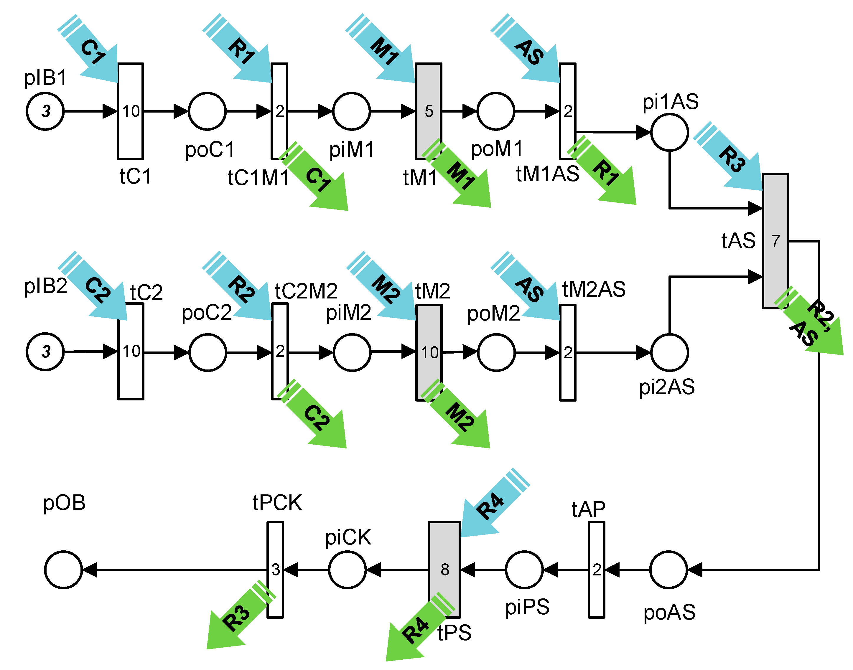
7.2. Phase II: Adding the Run-Time Dynamics
The second phase of the AOPN approach is the addition of the run-time dynamics on the static Petri Net graph to make it the initial dynamic Petri net model. For example, the details about the activities requesting, using, and releasing a variety of resources are added in the second phase [6,26]. The initial markings of the places and the firing times of the transitions are also added in the second phase.
Table 3, given below, shows the activities and the resources used by these activities.
Figure 4 shows the Petri net model obtained after Phase II of the AOPN approach. The dynamic model shows the resources required by the different transitions and the resources released after firing. Also shown in Figure 4 are the initial markings of the places and the firing times of the transitions.
8. Simulation with GPenSIM
In this section on coding and simulations, the first subsection presents some of the useful functions in GPenSIM for modeling scheduling problems with the AOPN approach. The second subsection presents the implementation details of the FMS example.
8.1. Scheduling Using GPenSIM
There are some issues in the scheduling of resources:
- Instances of a resource: A resource can have many indistinguishable copies (“instances”), e.g., there are three cashiers in a shop (resource cashier has three instances). For a customer, it does not make sense to prefer one cashier over the others. In this case, we could generalize all the cashiers into a group, name this resource as “cashier”, and say that cashier is a single resource with three instances.
- Generic resources: There are some “named” resources available, but all of them are the same for some specific applications, e.g., in a mechanical workshop, there are three mechanics named “Alan”, “Bobby”, and “Chan”; though they are specialists in some works, when it comes to engine repair, they all are the same. Thus, for engine repair, we can pick a generic mechanic, without specifically naming anyone.
- Specific resources: When the resources are named, we may request specific (named) resources. For example, in the mechanical workshop, “Chan” is an electrician. Hence, when we need an electrical fixing, we would prefer to use the specific resource “Chan”.
- Write Access: When a resource has many instances, a transition may try to acquire one or many of these instances. Write access means that the resource will be locked, and all the instances will be made available to a requesting transition.
Table 4 shows a number of GPenSIM functions available for the modeling of resource scheduling.
8.2. Code Implementation with GPenSIM
As discussed in the Section 3 and Section 4, implementing a Petri net model using GPenSIM usually results in four files: the main simulation file (MSF), the Petri net Definition file (PDF), and the two common processor files (COMMON_PRE file and COMMON_POST file).
The PDF file given below defines the static Petri net graph by declaring the sets of places, transitions, and arcs.
PDF:
% PDF: 'fms_AOPN_pdf.m'
function [png] = fms_AOPN_pdf()
png.PN_name = 'AOPN model of a FMS';
png.set_of_Ps = {'pIB1','pIB2', 'pOB',... %input & output buffers
'poC1','poC2','piM1','piM2','poM1', 'poM2', ...%intermediate buffers
'pi1AS','pi2AS','poAS', 'piPS','piCK'}; %intermediate buffers
png.set_of_Ts = {'tC1','tC2', 'tC1M1','tC2M2', 'tM1','tM2',...
'tM1AS','tM2AS','tAS', 'tAP', 'tPS', 'tPCK'};
png.set_of_As = {'pIB1','tC1',1, 'tC1','poC1',1, ... % tC1 connections
'poC1','tC1M1',1, 'tC1M1','piM1',1, ... % tC1M1 connections
'piM1','tM1',1, 'tM1','poM1',1,... % tM1 connections
'poM1','tM1AS',1, 'tM1AS','pi1AS',1,... % tM1AS connections
'pIB2','tC2',1, 'tC2','poC2',1, ... % tC2 connections
'poC2','tC2M2',1, 'tC2M2','piM2',1,... % tC2M2 connections
'piM2','tM2',1, 'tM2','poM2',1,... % tM2 connections
'poM2','tM2AS',1, 'tM2AS','pi2AS',1,... % tM2AS connections
'pi1AS','tAS',1,'pi2AS','tAS',1, 'tAS','poAS',1,... % tAS connections
'poAS','tAP',1, 'tAP','piPS',1,... % tAP connections
'piPS','tPS',1, 'tPS','piCK',1, ... % tPS connections
'piCK','tPCK',1, 'tPCK','pOB',1}; % tPCK connections
The MSF is shown below. In the MSF, firstly, the initial dynamics (e.g., initial tokens in places, firing times of transitions, available system resources) are declared. Then, the simulation iterations are started by calling the function “gpensim”. When the simulation iterations are complete, the results can be plotted (graphics) or displayed.
MSF:
% MSF: 'fms_AOPN.m'
% AOPN model of a Flexible Manufacturing System
global global_info
global_info.STOP_AT = 300;
pns = pnstruct('fms_AOPN_pdf'); % the PDF file
dp.m0 = {'pIB1',3,'pIB2',3}; % initial markings on the places
dp.ft = {'tC1',10,'tC2',10,'tM1',5,'tM2',10,... % firing times
'tAS',7,'tPS',8, 'tPCK',3, 'allothers',2}; % firing times
dp.re = {'C1',1,inf,'C2',1,inf, 'M1',1,inf,'M2',1,inf, ... % resources
'R1',1,inf,'R2',1,inf,'R3',1,inf,'R4',1,inf}; % resources
pni = initialdynamics(pns, dp); % initial run-time PetriNet
sim = gpensim(pni); % simulation iterations
prnschedule(sim); % print the simulation results
The common processor file COMMON_PRE declares the resources required by the enabled transitions to start firing, whereas COMMON_POST declares the resources released by the fired transitions. The information coded in these two files is the same information that is presented in Table 3 in a tabular format.
COMMON_PRE:
function [fire, transition] = COMMON_PRE(transition)
switch transition.name
case'tC1', granted = requestSR({'C1',1});
case'tC1M1', granted = requestSR({'R1',1});
case'tM1', granted = requestSR({'M1',1});
case'tC2', granted = requestSR({'C2',1});
case'tC2M2', granted = requestSR({'R2',1});
case'tM2', granted = requestSR({'M2',1});
case'tAS', granted = requestSR({'R3',1});
case'tPS', granted = requestSR({'R4',1});
case {'tM1AS','tM2AS', 'tAP','tPCK'}, granted = 1; % request nothing
end % switch
fire = granted; % fire if the required resource is granted
COMMON_POST:
function [] = COMMON_POST(transition)
switch transition.name
case'tC1' % do nothing
case'tC1M1', release('tC1'); % release resource acquired by tC1
case'tM1', release(); % release resource acquired by tM1
case'tM1AS', release('tC1M1'); % release resource acquired by tC1M1
case'tC2' % do nothing
case'tC2M2', release('tC2'); % release resource acquired by tC2
case'tM2', release(); % release resource acquired by tM2
case'tM2AS'% do nothing
case'tAS', release('tC2M2');
case'tAP' % do nothing
case'tPS', release(); % 'R4'
case'tPCK', release('tAS');
end % switch
n = ntokens('pOB'); % get the number of tokens in pOB
if eq(n,3), global_info.STOP_SIMULATION = 1; end % stop if n==3
8.3. Simulation Result
The simulation result given below is for the production of three units of products, as the simulation was started with three initial tokens in each of the places pIB1 and pIB2. The simulation result gives a very detailed analysis of the resource usage. Also, if the transitions (activities) and the resources are assigned costs (fixed costs and variable costs), the final costs of the products would be displayed in the result; however, the costs are neglected (assigned zero value) in this example.
Simulation results
RESOURCE USAGE:
RESOURCE INSTANCES OF ***** C1 *****
tC1 [0 : 12]
tC1 [12 : 24]
tC1 [24 : 36]
Resource Instance: C1:: Used 3 times. Utilization time: 36
RESOURCE INSTANCES OF ***** C2 *****
tC2 [0 : 12]
tC2 [12 : 33]
tC2 [33 : 54]
Resource Instance: C2:: Used 3 times. Utilization time: 54
RESOURCE INSTANCES OF ***** M1 *****
tM1 [12 : 17]
tM1 [24 : 29]
tM1 [36 : 41]
Resource Instance: M1:: Used 3 times. Utilization time: 15
RESOURCE INSTANCES OF ***** M2 *****
tM2 [12 : 22]
tM2 [33 : 43]
tM2 [54 : 64]
Resource Instance: M2:: Used 3 times. Utilization time: 30
RESOURCE INSTANCES OF ***** R1 *****
tC1M1 [10 : 19]
tC1M1 [22 : 31]
tC1M1 [34 : 43]
Resource Instance: R1:: Used 3 times. Utilization time: 27
RESOURCE INSTANCES OF ***** R2 *****
tC2M2 [10 : 31]
tC2M2 [31 : 52]
tC2M2 [52 : 73]
Resource Instance: R2:: Used 3 times. Utilization time: 63
RESOURCE INSTANCES OF ***** R3 *****
tAS [24 : 44]
tAS [45 : 65]
tAS [66 : 86]
Resource Instance: R3:: Used 3 times. Utilization time: 60
RESOURCE INSTANCES OF ***** R4 *****
tPS [33 : 41]
tPS [54 : 62]
tPS [75 : 83]
Resource Instance: R4:: Used 3 times. Utilization time: 24
RESOURCE USAGE SUMMARY:
C1: Total occasions: 3 Total Time spent: 36
C2: Total occasions: 3 Total Time spent: 54
M1: Total occasions: 3 Total Time spent: 15
M2: Total occasions: 3 Total Time spent: 30
R1: Total occasions: 3 Total Time spent: 27
R2: Total occasions: 3 Total Time spent: 63
R3: Total occasions: 3 Total Time spent: 60
R4: Total occasions: 3 Total Time spent: 24
***** LINE EFFICIENCY AND COST CALCULATIONS: *****
Number of servers: k = 8
Total number of server instances: K = 8
Completion = 86
LT = 688
Total time at Stations: 309
LE = 44.9128 %
**
Sum resource usage costs: 0 (NaN% of total)
Sum firing costs: 0 (NaN% of total)
Total costs: 0
**
9. Discussion
General-purpose Petri Net Simulator (GPenSIM) is a software for the modeling, simulation, performance analysis, and control of discrete event systems. GPenSIM, developed by the first author of this paper, runs on the MATLAB platform. Though GPenSIM is new, it has been accepted by some universities around the world because of its simplicity, flexibility, and for the possibilities of interaction with the other MATLAB toolboxes and the external environment. GPenSIM (current version 9) can be freely downloaded from the website [4].
GPenSIM is being used to solve many engineering problems. For example, Service-Oriented Architecture [9], Solving Repetitive Production Planning Problems [26], Assembly Line Balancing Problems [27], Gameplay [11], Flexible Manufacturing Systems [12], Service Modeling [13], and Complex Interconnected Manufacturing Systems [10]. With GPenSIM, control of external hardware is also possible, e.g., a logical control system of a marine diesel engine [7], control of Atlantic salmon farming industry processes [28], and real-time control of a humanoid robot [8]. Finally, being a MATLAB toolbox, GPenSIM is used for integrating Petri net models with the other MATLAB toolboxes, e.g., with a Neural Network to make a learning Petri net model [29], with Fuzzy Logic to make Fuzzy Petri nets [30], and integration with the RWTH Lego NXT toolbox for real-time control of Lego robots [28].
9.1. Gpensim Is Not Only for Event Graphs
In the first half of this paper, the focus was given to strongly connected event graphs. The performance of a strongly connected event graph can easily be evaluated using the functions available in GPenSIM. The paper starts with the Event Graph, which is a particular class of Petri nets (defined in Section 4.1), that possess the properties defined in Section 4.2. The materials presented in Section 4.1 and Section 4.2 are for event graphs only.
However, the application of GPenSIM is not limited to event graphs. As stated in Section 2, GPenSIM supports nearly all the well-known Petri net classes and extensions (including inhibitor arcs, color extension, enabling functions, priorities, etc.). Since GPenSIM is flexible, other ad hoc extensions can also be easily implemented in GPenSIM.
9.2. The Advantages of the AOPN Approach
The AOPN approach presented in Section 3 and Section 7 can be used to simplify Petri net models of discrete event systems, especially ones with a large number of system resources. The AOPN approach can be used to obtain compact models, and the functions available in GPenSIM can be used for performance evaluation. For reproducibility, the complete code for the simulations shown in the paper is available from the website [25]; the interested reader is encouraged to download the code and experiment with it.
To understand the advantage of the AOPN approach from the example given in this paper, we have to compare Figure 2 (Timed Petri net model) with Figure 3 (AOPN model). Figure 4 shows the run-time model where the arrows labeled “C1” and “R1” show the transitions requesting and releasing resources during run-time. Again, by comparing Figure 2 and Figure 3, we can see that the AOPN approach provides compact models. Because of the compact models (fewer places and arcs), the Petri net models run faster during simulations. However, this is only a secondary advantage.
The main advantage of the AOPN approach is the following. For the AOPN approach, as GPenSIM provides resource management support during simulations (managing resource reservations, allocations, and retrievals), GPenSIM also provides a detailed analysis of the resource usage, which is not possible by simply running a Petri net as in the case of the other Petri net simulators.
Author Contributions
Conflicts of Interest
The authors declare no conflict of interest.
References
- Peterson, J.L. Petri Net Theory and the Modeling of Systems; Prentice-Hall: Englewood Cliffs, NJ, USA, 1981. [Google Scholar]
- Proth, J.M. Performance evaluation of manufacturing systems. In Practice of Petri Nets in Manufacturing; Springer: Dordrecht, The Netherlands, 1993; pp. 147–183. [Google Scholar]
- Commoner, F.; Holt, A.W.; Even, S.; Pnueli, A. Marked directed graphs. J. Comput. Syst. Sci. 1971, 5, 511–523. [Google Scholar] [CrossRef]
- GPenSIM: A General Purpose Petri Net Simulator. Available online: http://www.davidrajuh.net/gpensim (accessed on 15 December 2017).
- Davidrajuh, R. Developing a new Petri net tool for simulation of discrete event systems. In Proceedings of the IEEE Second Asia International Conference on Modeling & Simulation (AICMS 08), Kuala Lumpur, Malaysia, 13–15 May 2008; pp. 861–866. [Google Scholar]
- Davidrajuh, R. Modeling Discrete-Event Systems with GPenSIM: An Introduction; Springer: Dordrecht, The Netherlands, 2018. [Google Scholar]
- Pan, X.L.; He, G.; Zhang, C.J.; Ming, T.F.; Wang, X.C. Research on Modeling and Simulating of Discrete Event System Based on Petri Net. In Advanced Engineering Forum; Trans Tech Publications: Zürich, Switzerland, 2012; Volume 4, pp. 80–85. [Google Scholar]
- Davidrajuh, R. Modeling Humanoid Robot as a Discrete Event System: A Modular Approach Based on Petri Nets. In Proceedings of the IEEE 2015 3rd International Conference on Artificial Intelligence, Modelling and Simulation (AIMS), Sabah, Malaysia, 2–4 December 2015. [Google Scholar]
- Cameron, A.; Stumptner, M.; Nandagopal, N.; Mayer, W.; Mansell, T. Rule-based peer-to-peer framework for decentralised real-time service oriented architectures. Sci. Comput. Program. 2015, 97, 202–234. [Google Scholar] [CrossRef]
- Lopez, F.; Barton, K.; Tilbury, D. Simulation of Discrete Manufacturing Systems with Attributed Hybrid Dynamical Nets. Unpublished work. 2017. [Google Scholar]
- Chang, H. A Method of Gameplay Analysis by Petri Net Model Simulation. J. Korea Game Soc. 2015, 15, 49–56. [Google Scholar] [CrossRef]
- Jyothi, S.D. Scheduling Flexible Manufacturing System Using Petri-Nets and Genetic Algorithm; Department of Aerospace Engineering, Indian Institute of Space Science and Technology: Thiruvananthapuram, India, 2012. [Google Scholar]
- Hussein, L.Z.S. Simulation of Food Restaurant Using Colored Petri Nets. J. Eng. Dev. 2014, 18, 77–88. [Google Scholar]
- Sanders, W.H.; Meyer, J.F. Stochastic activity networks: Formal definitions and concepts. In School Organized by the European Educational Forum; Springer: Berlin/Heidelberg, Germany, 2000; pp. 315–343. [Google Scholar]
- Davidrajuh, R. Activity-Oriented Petri Net for Scheduling of Resources. In Proceedings of the 2012 IEEE International Conference on Systems, Man, and Cybernetics, Seoul, Korea, 14–17 October 2012. [Google Scholar]
- Davidrajuh, R. Representing Resources in Petri Net Models: Hardwiring or Soft-coding? In Proceedings of the 2011 IEEE International Conference on Service Operations and Logistics, and Informatics, Beijing, China, 10–12 July 2011. [Google Scholar]
- Davidrajuh, R. Scheduling using ‘Activity-based Modeling’. In Proceedings of the 2011 IEEE Conference on Computer Applications & Industrial Electronics (ICCAIE 2011), Penang, Malaysia, 4–7 December 2011. [Google Scholar]
- Wu, N.; Zhou, M. System Modeling and Control with Resource-Oriented Petri Nets; CRC Press: New York, NY, USA, 2010. [Google Scholar]
- Zhou, M.C.; DiCesare, F. Parallel and sequential mutual exclusions for Petri net modeling of manufacturing systems with shared resources. IEEE Trans. Robot. Autom. 1991, 7, 515–527. [Google Scholar] [CrossRef]
- Chretienne, P. Exécutions controlées des réseaux de Petri temporisés. TSI Tech. Sci. Inform. 1984, 3, 23–31. [Google Scholar]
- Cormen, T.H. Introduction to Algorithms; MIT Press: Cambridge, MA, USA, 2009. [Google Scholar]
- Rader, C.M. Connected components and minimum paths. In Graph Algorithms in the Language of Linear Algebra; Jeremy, K., Gilbert, J., Eds.; SIAM Publications: Philadelphia, PA, USA, 2011. [Google Scholar]
- Tiernan, J.C. An efficient search algorithm to find the elementary circuits of a graph. Commun. ACM 1970, 13, 722–726. [Google Scholar] [CrossRef]
- Johnson, D.B. Finding all the elementary circuits of a directed graph. SIAM J. Comput. 1975, 4, 77–84. [Google Scholar] [CrossRef]
- Complete Code for the Examples. Available online: http://www.davidrajuh.net/gpensim/Pub/2018/computers-j/ (accessed on 15 December 2017).
- Skolud, B.; Krenczyk, D.; Davidrajuh, R. Solving Repetitive Production Planning Problems. An Approach Based on Activity-oriented Petri Nets. In Advances in Intelligent Systems and Computing, Proceedings of the International Joint Conference SOCO’16-CISIS’16-ICEUTE’16 (ICEUTE 2016, SOCO 2016, CISIS 2016), San Sebastián, Spain, 19–21 October 2016; Springer: Cham, Switzerland, 2017; Volume 527, pp. 397–407. [Google Scholar]
- Davidrajuh, R. Solving Assembly Line Balancing Problems with Emphasis on Cost Calculations: A Petri nets Based Approach. In Proceedings of the IEEE Modelling Symposium (EMS), Pisa, Italy, 21–23 October 2014; pp. 99–104. [Google Scholar]
- Davidrajuh, R. Developing a petri nets based real-time control simulator. Int. J. Simul. Syst. Sci. Technol. IJSSST 2012, 12, 28–36. [Google Scholar]
- Fadhilah, R. Fuzzy Petri Nets as a Classification Method for Automatic Speech Intelligibility Detection of Children with Speech Impairments. Ph.D. Thesis, University of Malaya, Kuala Lumpur, Malaya, 2016. [Google Scholar]
- Melberg, R. Modeling, Simulation, and Control of Atlantic Salmon Farming Industry Processes. Ph.D. Thesis, University of Stavanger, Stavanger, Norway, 2010. [Google Scholar]
Figure 1.
The Flexible Manufacturing System (FMS).
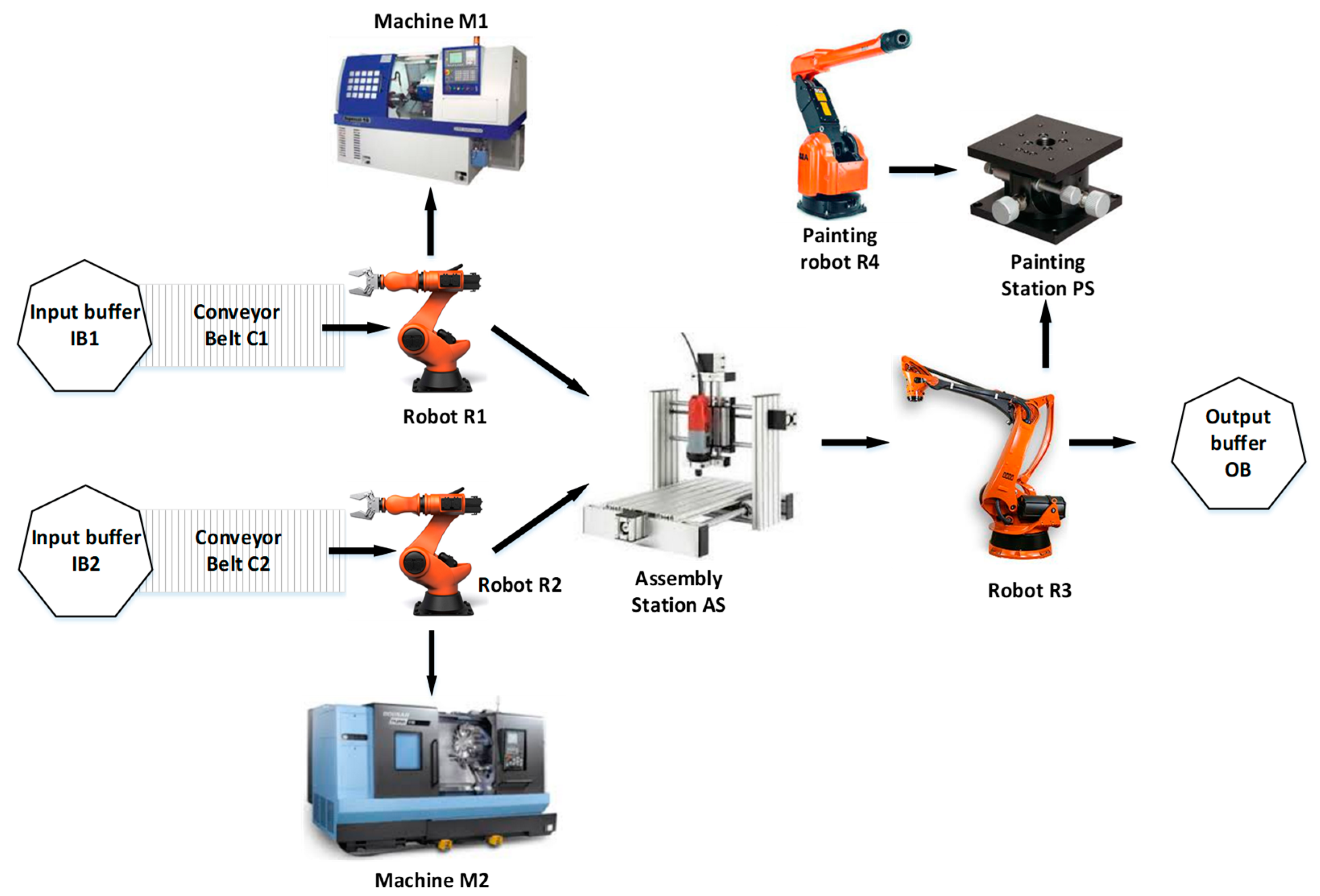
Figure 2.
Petri Net model of the FMS.
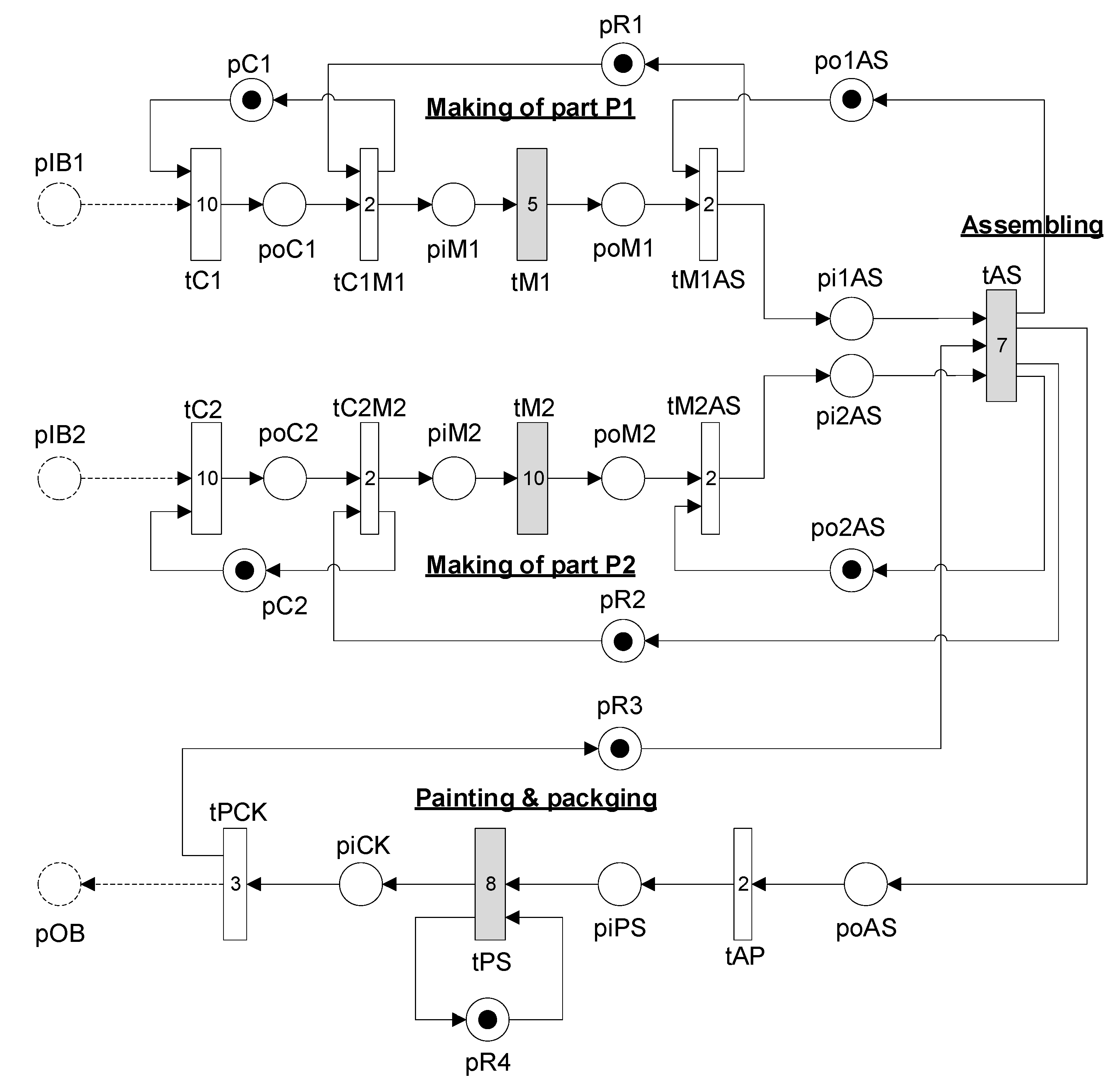
Figure 3.
The compact Petri Net model obtained by Phase I of the AOPN approach.
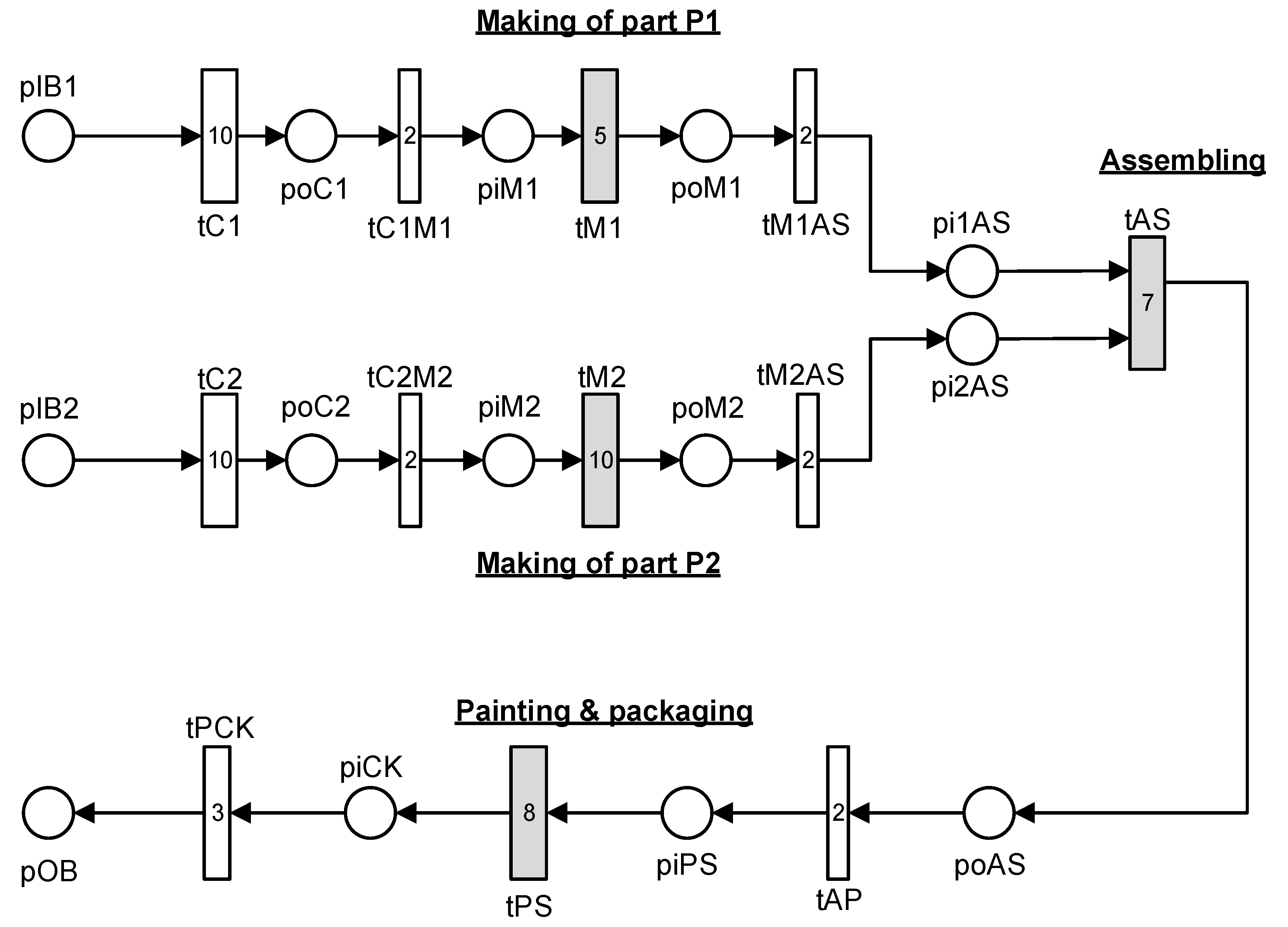
Figure 4.
The run-time Petri Net model obtained by Phase II of the AOPN approach.


Table 1.
Summary: Comparing Process-Oriented Petri Nets (POPN), Resource-OPN (ROPN), and Activity-OPN (AOPN).
Table 1.
Summary: Comparing Process-Oriented Petri Nets (POPN), Resource-OPN (ROPN), and Activity-OPN (AOPN).
| POPN [18] | ROPN [19] | AOPN [15] | |
|---|---|---|---|
| Number of places | O(n + r) | O(r) | O(n) |
| Number of transitions | O(n) | O(r2) | O(n) |
Table 2.
General-purpose Petri Net Simulator (GPenSIM) functions for performance evaluation of strongly connected event graphs (SCEG).
Table 2.
General-purpose Petri Net Simulator (GPenSIM) functions for performance evaluation of strongly connected event graphs (SCEG).
| GPenSIM Function | Purpose |
|---|---|
| pnclass | Find out the class of Petri net |
| stronglyconn | Find out the number of strongly connected components in the Petri net |
| mincyctime | Finding the performance bottleneck in a SCEG |
| cycles | Extract the elementary circuits in a Petri Net |
Table 3.
The activities and the resources used by these activities.
| Transition | Resources Required to Start Firing | Resources Released After Firing |
|---|---|---|
| tC1 | C1 | - |
| tC1M1 | R1 | C1 (acquired by tC1) |
| tM1 | M1 | M1 |
| tM1AS | - | R1 (acquired by tC1M1) |
| tC2 | C2 | - |
| tC2M2 | R2 | C2 (acquired by tC2) |
| tM2 | M2 | M2 |
| tM2AS | - | - |
| tAS | R3 | R2 (acquired by tC2M2) |
| tAP | - | - |
| tPS | R4 | R4 |
| tPCK | - | R3 (acquired by tAS) |
Table 4.
GPenSIM functions for the modeling of resource scheduling.
| GPenSIM Function | Purpose |
|---|---|
| availableInst | check whether any instances are available in a resource |
| availableRes | check whether any resources are available (not in use) |
| requestsSR | request a number of instances from specific (“named“) resources |
| requestGR | request a number of resource instances, without naming any re-source |
| requestAR | request a number of resource instances among many alternatives |
| requestWR | request all the instances of a specific resource (either all or none) |
| release | release all the resources and resource instances held by a transition |
| Prnschedule | prints information on resource usage |
© 2018 by the authors. Licensee MDPI, Basel, Switzerland. This article is an open access article distributed under the terms and conditions of the Creative Commons Attribution (CC BY) license (http://creativecommons.org/licenses/by/4.0/).
Share and Cite
MDPI and ACS Style
Davidrajuh, R.; Skolud, B.; Krenczyk, D. Performance Evaluation of Discrete Event Systems with GPenSIM. Computers 2018, 7, 8. https://doi.org/10.3390/computers7010008
AMA Style
Davidrajuh R, Skolud B, Krenczyk D. Performance Evaluation of Discrete Event Systems with GPenSIM. Computers. 2018; 7(1):8. https://doi.org/10.3390/computers7010008
Chicago/Turabian StyleDavidrajuh, Reggie, Bozena Skolud, and Damian Krenczyk. 2018. "Performance Evaluation of Discrete Event Systems with GPenSIM" Computers 7, no. 1: 8. https://doi.org/10.3390/computers7010008
Note that from the first issue of 2016, this journal uses article numbers instead of page numbers. See further details here.