The Influence of Priming on Reference States

Max-Planck-Institute of Economics, Kahlaische Str. 10, D-07745 Jena, Germany
Games 2010, 1(1), 34-52; https://doi.org/10.3390/g1010034
Submission received: 27 January 2010
/
Revised: 8 March 2010
/
Accepted: 12 March 2010
/
Published: 16 March 2010
Abstract
:Experimental and empirical evidence shows that the utility an individual derives from a certain state depends on the reference state she compares it to. According to economic theory, the reference state is determined by past, present and future outcomes of either the individual herself or her reference group. The experiment described in this paper suggests that, in addition, reference states depend to a significant degree on environmental factors not relevant for outcomes. It indicates that reference states - and hence utility - can relatively easily be influenced without changing people’s outcomes, e.g., through priming.
1. Introduction
Can individual utility change if outcomes and expectations remain constant? According to economic theory, the answer is no: Individuals derive utility from their current [1] or future outcomes [2], which they compare to their reference state [3,4,5]. The reference state is also determined by outcomes, e.g., the outcomes the individual received in the past [6], the outcomes relevant others receive [7], the outcomes the individual expects [8], etc. As long as none of these outcomes changes, reference states and individual utility do not change.
The experiment described in this paper adds a new component to this theory: It suggests that reference states depend to a significant degree on the cues that individuals encounter in their environment, even if these cues are neither outcome-relevant nor are individuals consciously aware of them. In addition, it implies that reference states are not fully determined "within" the individual, but can relatively easily be influenced from outside.
Participants in the experiment first completed a priming task (see e.g. [9,10,11]. Each subject was primed with one of three concepts: a concept focusing on material achievements, a neutral concept, or a concept focusing on social achievements. The priming neither affected participants’ outcomes, nor did it reveal any outcome-relevant information, nor were participants aware of being primed. Afterwards, all subjects participated in a lottery where they could invest all or part of their endowment. Applying prospect theory [3], systematic differences in subjects’ investments were then used to identify differences in their reference states [12].
The main experiment was run as a pen-and-paper classroom experiment. In addition, a computerized laboratory experiment was conducted to account for technical limitations of the main experiment and provide further control. The results show that the investments of subjects who were primed with the concept focusing on material achievements differ significantly from those of the subjects who were primed with the social and neutral concepts. This suggests that the individuals’ reference states have changed as the result of encountering different environmental cues at the priming stage.
The findings have implications for economic theory and experimental methods. First, they suggest that reference states do not only depend on outcomes, but also on environmental factors that are not relevant for outcomes. Through these factors they are potential subject to manipulation. Second, the results provide further evidence that individual utility is not as stable as economic theory tends to assume. Earlier research has already identified influences on behavior that are not outcome-relevant, like framing [13] and anchoring (e.g. [14]). The results presented here suggest that even if preferences are stable and framing effects are absent, utility can vary widely depending on - supposedly - subtle environmental factors. Finally, the findings show that nuances of the design of economic experiments may lead to unintended priming effects and influence subjects’ reference states. This may render seemingly identical treatments or experiments non-comparable, and experimental results hard to interpret.
It should be noted that this study - as any research on reference states - suffers from the unobservability of its object. However, understanding the formation of reference states is crucial for the understanding of individual utility and decision making in a broad range of situations. This makes it worth accepting the methodological compromises involved in this kind of research. While in survey studies (e.g. [15,16]) this compromise involves accepting non-incentivized statements, in our case it involves accepting the indirect measurement of the variable of interest.
2. Experiment
2.1. Classroom experiment
The main experiment was run as a pen-and-paper classroom experiment. It consisted of two stages. At the first stage subjects completed a priming task. Priming is a method developed in (social) psychology to activate mental representations without drawing participants’ attention to this activation (see [17] for an early conceptualization of mental representations and their activation). Over the past 30 years a number of different priming techniques have been developed and their effects on a wide range of situations and decisions studied (see [9] for a recent review and discussion). This research suggests that priming subjects with a single concept can have a number of simultaneous effects, whose interaction is not yet fully understood. The analysis in this paper focuses on the effect of priming on subjects’ reference states.
Participants in the experiment were primed with three different concepts. They received 20 groups of five words each that they had to sort into meaningful phrases of four words. The instructions included one sample phrase. There were three treatments. Half of the phrases were of neutral content, e.g., “Trees have green leaves.”. These were the same in all treatments. The remaining phrases differed between treatments. In the first treatment (MAT), these phrases referred to material achievements, e.g., “Consultants earn high wages.” The second treatment (CONT) was a control treatment, which included only neutral phrases. In the third treatment (SOC), the non-neutral phrases referred to social achievements, e.g., “Volunteers help in sports clubs.”. All phrases referred to common knowledge items. It seems highly unlikely that they induced participants to update their expectations regarding their future income or wealth. In addition, pre-experimental tests with student assistants who completed the tasks but where otherwise ignorant of the design indicated that participants were not aware of being primed with specific concepts. This is in line with earlier experiments using priming (see, [10]). However, for technical reasons a formal funneled debriefing procedure [18] was not included in the classroom experiment.
The second stage was identical across treatments. People received an endowment of 5 Euro and could invest any amount between 0 and 5 Euro in a lottery. In this lottery, investments were tripled or lost, each with 50% chance. Amounts not invested were kept by the participants, i.e., the expected payoff was
In addition to stating their investments, participants were also asked for the minimum fixed amount of money they would have preferred over their participation in the lottery.
E(payoff) = 5 − investment + 0.5 ∗ 3 ∗ investment = 5 + 0.5 ∗ investment .
The experiment was conducted in two undergraduate lectures at the University of Jena in fall 2007. There were 193 participants overall. After participants had made their decisions, 25 of them were drawn randomly to be paid. Their lottery results were determined by flipping a coin, and payments were made after the lecture. All participants were aware of this procedure when making their decisions (See a translated version of the instructions in appendix B.).
2.2. Laboratory experiment
Tests conducted prior to the classroom experiment suggested that participants did not guess the purpose of the priming stage. However, as mentioned above, for technical reasons a formal debriefing stage ensuring that subjects did not guess the purpose of the study could not be included in the classroom experiment. Nor could subjects’ emotions be assessed to establish whether the priming stage affected subjects’ overall feelings (affective priming).1
To account for these limitations, a computerized control experiment was run in the laboratory of the Max-Planck-Institute (MPI) in Jena in February 2010. Due to the lab environment, the procedure differed somewhat from that of the classroom. Rather than being surprised by the experiment during an ordinary lecture, subjects were invited to participate in the experiment through ORSEE (Greiner, 2004). Upon arrival, they received detailed instructions, describing the different stages of the experiment and the structure of the lottery (see appendix C). Then they were asked to sort the words into meaningful phrases, and subsequently determined their investment in the lottery and the minimum amount they would have been satisfied with in place of the lottery.
As the final step, subjects filled in a detailed questionnaire. The first part assessed their emotional state using the Positive Affect and Negative Affect Scales (PANAS) developed by [19], i.e., 10-item mood scales that comprise the Positive and Negative Affect Schedule.2 The second part contained the funneled debriefing procedure established by [18], that is used in priming experiments to test for subjects’ naivety regarding the primed concept and the overall purpose of the study. In particular, subjects were asked what they thought the purpose of the experiment was, the question it tried to study, whether the different tasks were related, whether their behavior in one task was influenced by what they did in another, and whether they noted anything unusual or a certain theme or pattern in the groups of words.
After all subjects had completed the questionnaire, payments were made and the experiment ended. There were 92 participants in this experiment, all of them were paid according to the rules of the MPI lab. To ensure credibility of the procedure, lottery results were again determined by each participant flipping a coin.
Compared to the classroom environment, the laboratory is well suited to provide a controlled setup for the experiment, and to obtain all necessary data without running into technical or organizational problems. However, it also suffers from a number of limitations. The most relevant limitation for the purpose of the current experiment is that the laboratory environment itself serves as a (material) prime. The MPI advertises its experiments with a monetary argument, offering decent expected payoffs from the participation in its experiments. Accordingly, most participants take part for exactly this reason, which must be expected to affect the mind set in which they enter the lab. Further, since most of the participants in this experiment had already participated in earlier experiments, they had already experienced that MPI experiments offer the opportunity to earn substantial amounts of "easy" money. This may have enforced the monetary "priming" by the laboratory environment. Many statements that subjects’ made in post-experimental questionnaires of earlier experiments confirm this effect.
In addition, subjects may think that there is a (theoretically) "right" decision in the investment stage, since this is what they expect from the MPI and from experience in earlier experiments. Finally, in the laboratory the instructions already included a detailed plan of all stages of the experiment and enough time to think about them. This gave subjects the chance to plan their decisions in the lottery stage before even reading the groups of words, which may have provided an anchor for their later decisions. Several subjects explicitly stated in the questionnaire that they had made this decision before the experiment started. These limitations of the lab environment should be kept in mind when interpreting the results.
3. Background and Methodology
There is by now broad agreement in the literature that individual utility from realized outcomes depends on the individual’s outcome x and on the reference state r that she compares this outcome to (see [3]):3
There is, however, less agreement on how the reference state is formed. The most frequently suggested factors to influence r are: one’s own previous outcomes (status quo or habit formation, see e.g. [6,21]), the outcomes of relevant others (social comparison, e.g. [7]), one’s expected outcomes (e.g. [8,22]), or the outcomes one aspires for (e.g. [12,23,24,25]). As these examples show, models of reference formation assume the reference state to depend on the individual’s or relevant others’ outcomes, be them past, present, or future. Individual differences in the evaluation of these outcomes are captured by the functional forms of u and v, which are individual specific. However, u and v are assumed to be stable at least in the medium term. This means that although the form of u and v may change over a life-time, in the short-run individual utility depends only on the arguments of u and v, that is, on outcomes.
U(x) = u(x) + v(x|r)
The hypothesis that this paper is based on is that reference states - and hence utility - also depend on non-outcome relevant factors that individuals encounter in their environment. To test this hypothesis, the experiment systematically varies the cues that the subjects encounter at the priming stage, and attempts to identify differences in reference states that result from this variation. The way to identify these differences is through measuring differences in people’s risk attitudes. This approach has been used by [12], and is described in detail there. It is based on prospect theory, which suggests that loss averse individuals who face prospective losses take more risk than individuals who face prospective gains. This is due to the value function being concave for gains, but convex for losses (see [3]).
Given the same prospects, for individuals with higher reference states it is more likely that (some of) the possible outcomes are worse than their reference states. Accordingly, individuals with higher reference states are more likely to face losses from these prospects, and hence are less risk averse on average. Using this relation, and keeping the prospects that subjects can choose from the same across treatments, one can infer the influence of the different treatments on subjects’ reference states from the influence on their risk attitudes. In contrast to survey studies of reference state formation, one therefore does not have to rely on self-reports when determining whether the treatments lead to systematic differences in subjects’ reference states.
The argument is as follows: participants are randomly distributed across treatments. Since it is possible that students who sit in the first rows differ systematically from those who sit in the last rows, the treatments were distributed equally across rows. This means that subjects’ pre-experimental outcomes and reference states can be assumed to be randomly distributed. Participants in all treatments face the same lottery at stage two of the experiment, that is, a priori they face the same expected outcomes. Accordingly, past, present and expected future outcomes (given investments) do not differ systematically between treatments. The priming at stage one of the experiment intends to affect subjects’ reference states. If environmental cues systematically influence reference states, then the reference states of participants in different treatments will differ systematically. But if reference states differ systematically, then expected outcomes are also evaluated differently. According to the relation between prospective gains and losses on one hand, and risk attitudes on the other, this should be reflected in systematic differences in subjects’ risk attitudes between treatments. Hence, if one can find significant differences in average risk aversion between treatments, this implies that the treatments have influenced subjects’ reference states, and hence their utility.
It should be noted that an alternative interpretation of systematic differences in subjects’ risk attitude is possible, which is not based on reference states. Participants may distinguish between expected utility from income (EUI) and expected utility from terminal wealth (EUTW) (e.g. [26]). The broader the range of outcomes that they take into account when making their investment decision, the less risk averse subjects will be under a concave utility function. Hence, if the treatments lead to systematic differences in investments, this could suggest that environmental cues influence the range of outcomes that individual utility is based on.
Although this interpretation bears on a different theoretical effect than the one discussed above, the underlying argument is similar. In both cases, systematic differences in risk attitudes between treatments indicate that environmental cues influence the way individuals evaluate a given outcome, and the utility they derive from it. By focusing on the interpretation based on prospect theory, I therefore do not rule out alternative interpretations that are derived from this basic argument. Rather, prospect theory is chosen for the abundance of experimental and empirical evidence that exists in its support (see Section 1).
Further, the treatment could be suspected to influence risk attitudes directly, i.e., not by way of influencing reference states. This could be the case, e.g., if risky decisions were made in different domains, for which research has found domain-specific risk attitudes [27,28,29]. This is not the case here, since all investments are made according to the same instructions, i.e., in the same domain of lottery investments (see appendix). Similarly, investments preceding the ones we are analyzing, that could influence risk attitudes, i.e., through a house money effect (see [30,31]), are not present either.
Finally, differences in risk attitudes between treatments cannot be explained by framing effects. The part of the experiment that is related to the lottery and subjects’ investment decisions was formulated in exactly the same way in all three treatments. Hence, the investment decision was made given the same frame for all subjects. The two parts were also clearly separated in the instructions of the classroom experiment, with the lottery (the "game") appearing as a reward for the subjects rather than as part of the actual task (see instructions). The term ’experiment’ was not mentioned at either stage.
4. Results
4.1. Classroom experiment
The results are summarized in Table 1. Average and median investments are higher in the MAT treatment than in the CONT and SOC treatments. The difference between the MAT and the SOC treatments is statistically significant (Wilcoxon rank-sum test, p=0.0287). With 16% and 25%, respectively, the average and median differences in investments between the MAT and the SOC treatment are also non-negligible in size.
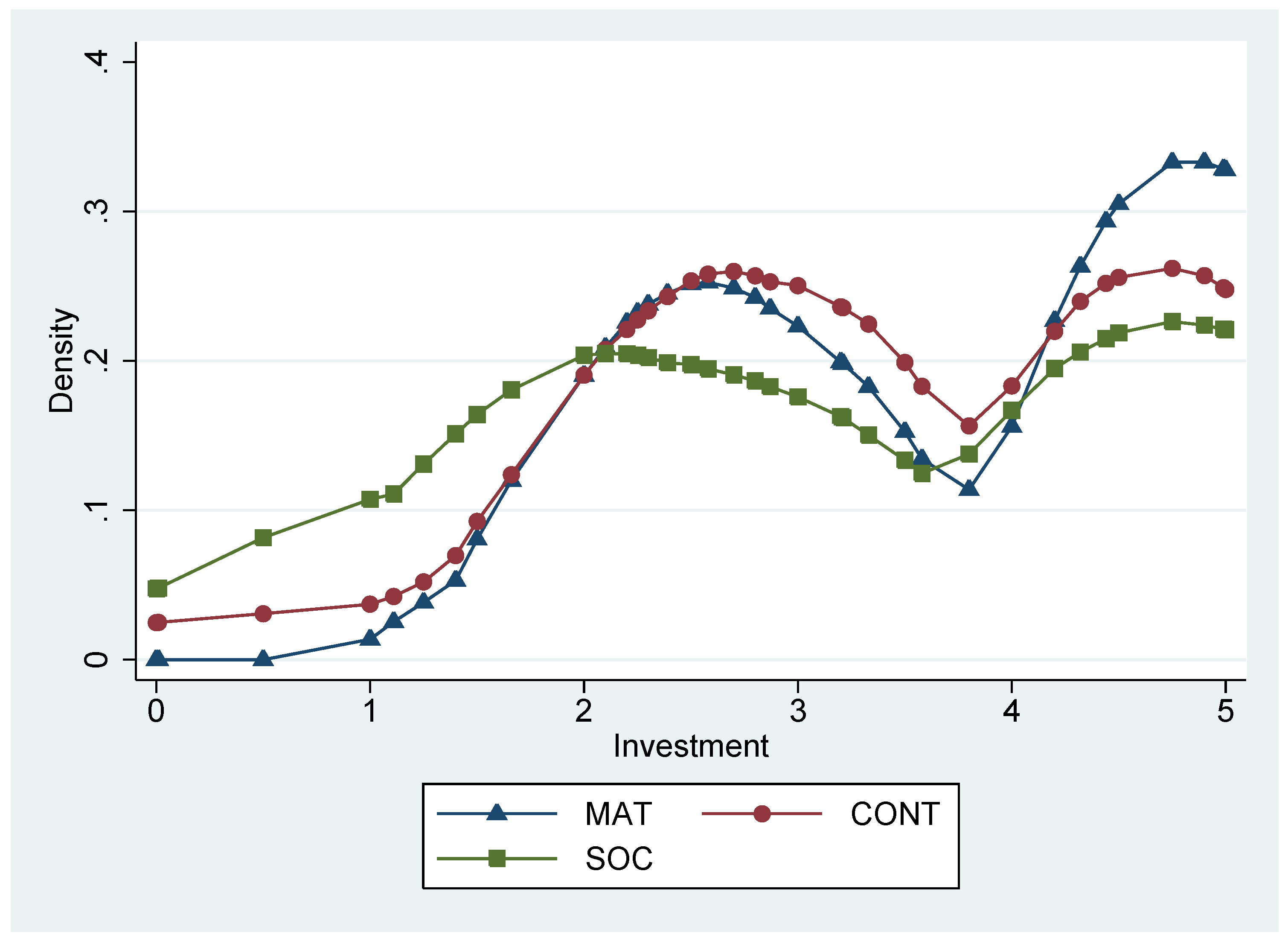
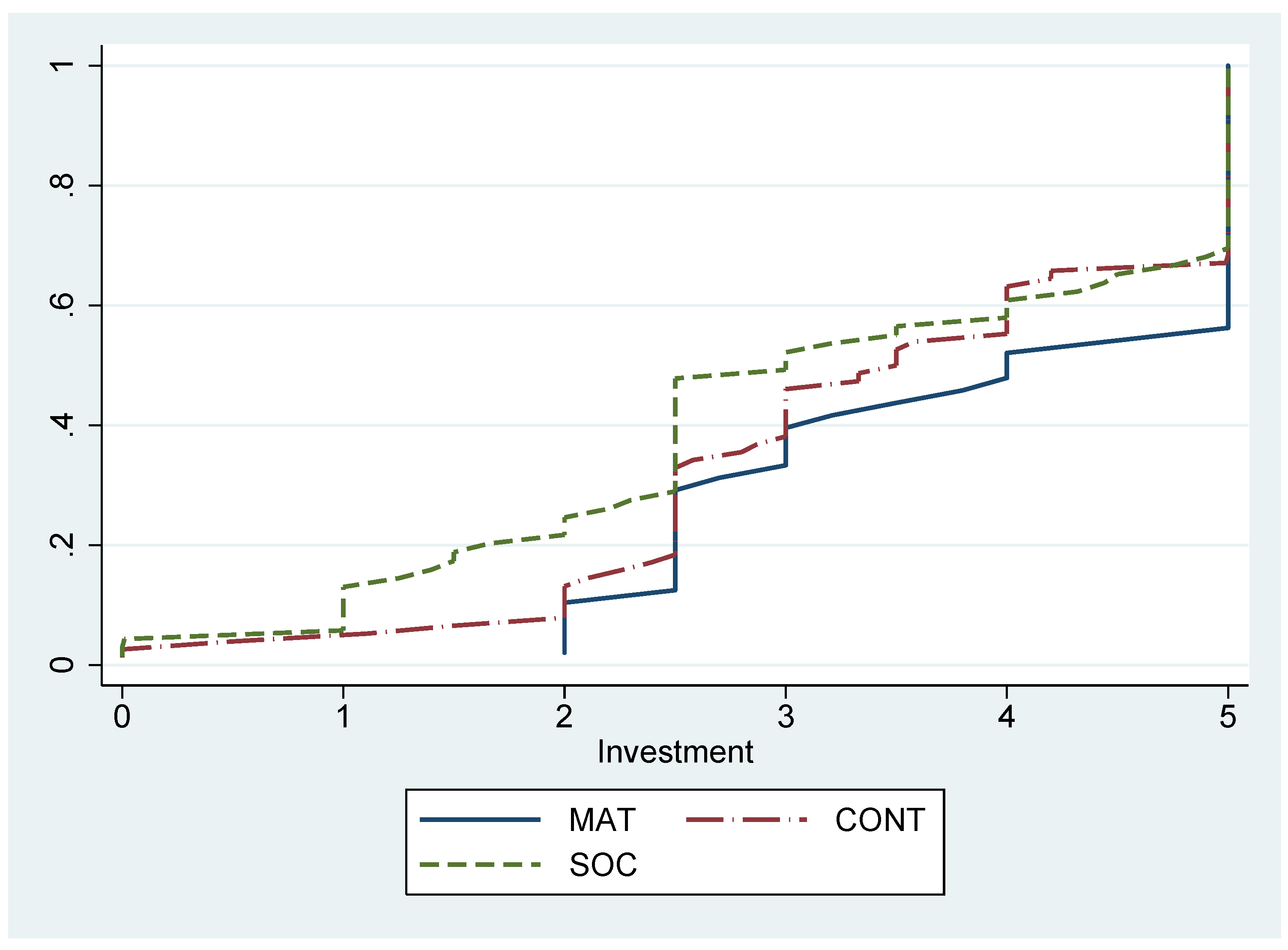
The distribution of individual investments is displayed in Figure 1 in the appendix. It indicates that the main differences between treatments arise at the tails of the distribution. Figure 2 shows that the cumulative distribution of the investment in the MAT treatment first-order stochastically dominates those of the CONT and SOC treatments. Further, it indicates that the cumulative distribution of the investment in the CONT treatment second-order stochastically dominates the one of the SOC treatment.
A similar picture arises for the minimum fixed amount people would have preferred over their participating in the lottery (`minimum’), with the caveat that these amounts were not incentivized. The differences in minimum amounts are significant between the MAT and SOC treatments (p=0.0087) and the MAT and CONT treatments (p=0.0041), but not between the SOC and CONT treatments (see also Figure 3 and Figure 4). This measure, in the way it was assessed similar to earlier survey research, offers additional support for a difference in reference states between treatments.
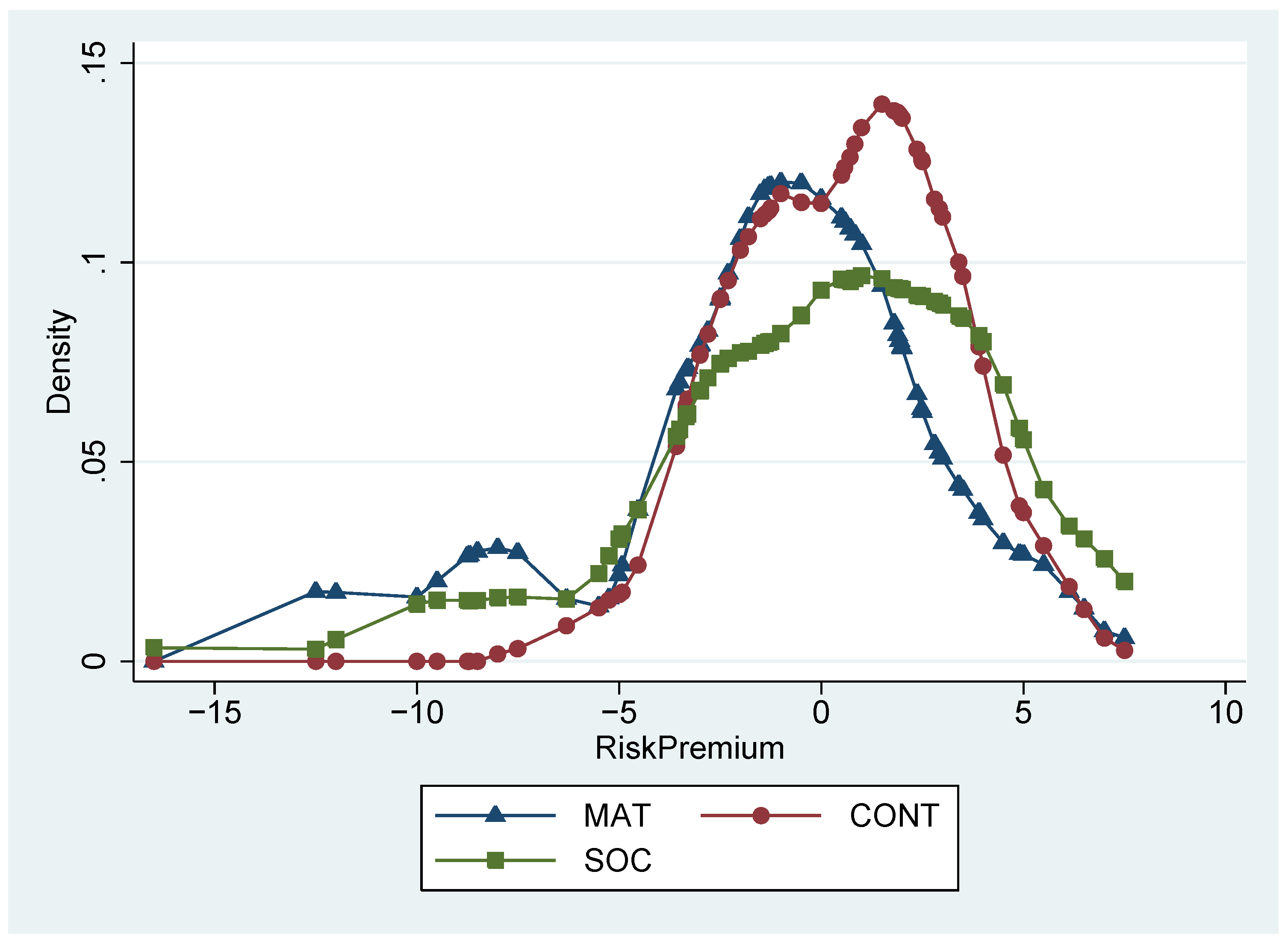
The risk premium, defined as the difference between the expected payoff given an individual’s investment and her minimum, is lower in the MAT treatment than in the CONT and SOC treatments. The Wilcoxon test shows again that the differences between the MAT and SOC treatments (p=0.0552) and the MAT and CONT treatments (p=0.0055) are statistically significant, but the difference between the CONT and SOC treatments is not (see Figure 5 for the distribution). Figure 6 shows that the cumulative distribution of the risk premium in the SOC treatment first-order stochastically dominates the one of the MAT treatment, which again is second-order stochastically dominated by the CONT treatment.
Regressions confirm the results of the non-parametric tests, also showing significant differences in investments and minimum amounts for the MAT, CONT and SOC treatments (1% level, see Table 2 in appendix A for details.).
When making their investment decisions, the participants in all three treatments faced the same situation, i.e., the same expected outcomes given their investments. Hence, the lower average risk aversion in the MAT treatment (higher investment, lower risk premium) implies that subjects in this treatment have a higher average reference state regarding monetary outcomes than subjects in the CONT and SOC treatments [3]. Since participants were randomly assigned to treatments, the difference in reference states can be attributed to subjects being exposed to different concepts at the priming stage.
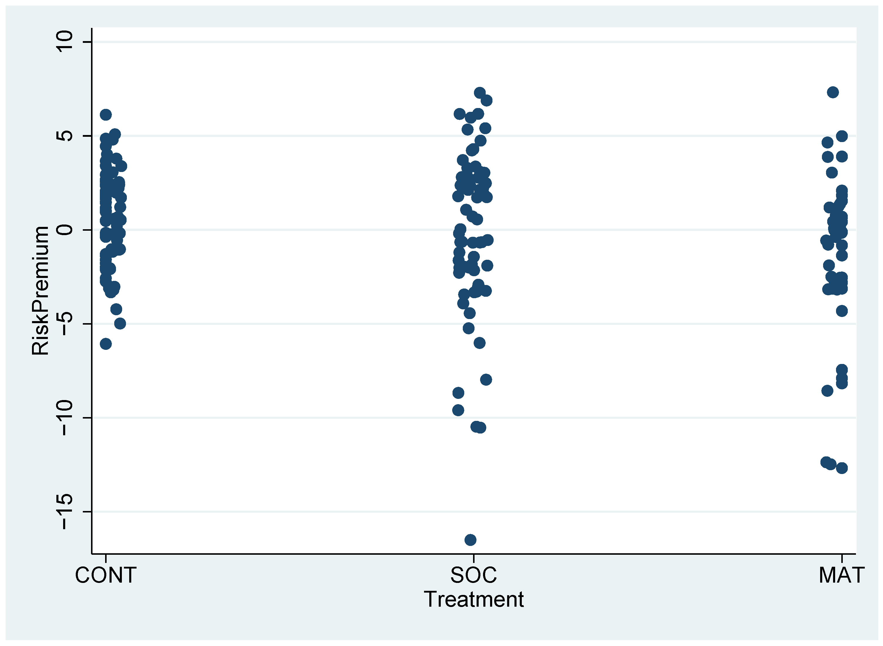
Another result is noteworthy: the standard deviation of the risk premium is significantly higher in the MAT and SOC treatments than in the CONT treatment (Variance ratio test, p < 0.001, see also Figure 7). This suggests that there may be different types of subjects that show different reactions to a particular environmental cue. For example, subjects with a generally social attitude may experience a weak or even resisting reaction when primed with the material concept, while subjects that generally focus more on material achievements may experience a strong enforcing reaction. In contrast, if the same subjects encounter social environmental cues, they may show opposite reactions.
4.2. Laboratory experiment
The results of the laboratory experiment regarding investment and minimum support those of the classroom experiment. Subjects in the material treatment show higher investments and ask for higher minimum fixed amounts than those in the control and social treatments. However, the differences are smaller than in the classroom experiment and only partly significant (see Table 3 in appendix A). This can be interpreted as an effect of the priming that occurs through the general environment in the lab of the MPI, and of the procedure that the rules of experimental economics require (in particular regarding the advertising of payments and the instruction phase).
The control mechanisms used in the lab suggest that the priming was done properly, and did not affect subjects’ general emotional state. As Table 4 in appendix A shows, subjects in the different treatments do not report significantly different emotions in the PANAS dimensions. Further, none of the 92 subjects correctly guessed the purpose of the study or reported that later decisions in the experiment were influenced by earlier stages. This is ensuring since in contrast to many priming experiments in psychology, the rules of experimental economics did not allow the use of a cover story in either experiment (classroom or lab).
In sum, the laboratory experiment confirms the conclusions of the classroom experiment, shows the correct functioning of the priming procedure and does not suggest the prevalence of an affective priming effect. However, it suggests that the general procedure in experimental economics, in particular the advertising of payments, may itself lead to a certain priming effect.
5. Discussion
The experiment shows that individuals’ reference states are influenced by the concepts they encounter in their environment. This leads to a change in utility and behavior, even if individuals are neither consciously aware of the different concepts, nor are their outcomes affected by them.
When interpreting the results, it should be taken into account that in the main experiment the priming took place in the noisy environment of a classroom experiment, where participants’ concentration on the task is naturally limited. Further, communication between participants of different treatments could not be avoided completely, which must be expected to lead to a reduction in the treatment effects. In addition, the priming phase took only about five minutes, since constructing the phrases was fairly straightforward. The significant differences between treatments that arise in spite of these constraints point to the large potential effect that exposure to different concepts in one’s environment may have on reference states, and hence on individual utility and behavior.
The findings have three major implications. First, they offer additional insights into the formation of reference states. In particular, they suggest that apart from an individual’s own past, present and expected future outcomes and the outcomes of relevant others, reference states also depend on environmental factors that do not influence outcomes. This makes them potential subject to manipulation by intentional or unintentional provision of environmental cues. Second, the results provide further evidence that a purely outcome-based model of individual utility may be incomplete, and may lead to unexplained differences in welfare and behavior. Finally, they show that when conducting experiments in economics, even small nuances of the instructions or design can influence subjects’ reference states and hence their behavior. This can render the results non-comparable to other experiments, and hard to interpret in absolute terms. In addition, the results of the laboratory environment suggest that the way experiments in economics are frequently conducted may have a significant priming effect itself, which may need to be taken into account when interpreting such evidence.
The results of the experiment are preliminary and further research is needed for substantiation. However, if the findings can be confirmed by future studies, they have implications for policy. In particular, they suggest that individuals who encounter less emphasis on material achievements in their environment have on average lower reference states regarding these achievements. They derive higher utility from any given level of material consumption. Put differently, with lower reference states a given level of utility requires less material achievements. This makes it easier for individuals to accept lower levels of consumption, or slower rises in material living standards. In times of shrinking natural resources, this may eventually contribute to a sustainable use of these resources without compromising individual utility.
Finally, two limitations of the study should be mentioned. First, as most experimental studies, it was conducted with students rather than with a representative sample of the population. Second, the effect on reference states was measured less than ten minutes after the priming, and it is hard to predict to what extent it would persist in the medium-term. Both points should be addressed in future studies before the results can be generalized.
Supplementary materials
Supplementary File 1Supplementary File 2Supplementary File 3Acknowledgements
I thank two anonymous referees, Vincent Crawford, Oliver Kirchkamp, Tobias Regner, Ondřej Rydval, seminar participants at University of Jena and Max-Planck-Institute of Economics, and participants in the IAREP/SABE Meeting 2008, the ESI-EVA Workshop 2008, the 4th European Conference on Positive Psychology, and the Conference on Economic De-growth 2008, for helpful comments. Research assistance by Tobias Regner, Michael Brodrecht, Adrian Liebtrau and Markus Heinemann is gratefully acknowledged.
Appendix A - Data

| MAT | CONT | SOC | ||
|---|---|---|---|---|
| investment | mean | 3.84 | 3.48 | 3.23 |
| median | 4 | 3.5 | 3 | |
| minimum | mean | 7.9 | 5.48 | 5.86 |
| median | 7.5 | 5 | 5 | |
| risk premium | mean | -1.57 | 0.55 | 0.14 |
| median | -0.5 | 0.58 | 0 | |
| observations | 48 | 75 | 69 |
Table 2.
Classroom experiment: Tobit (investment) and OLS (minimum) regressions with investment and minimum as dependent variables and robust standard errors
| investment | minimum | |||
|---|---|---|---|---|
| coeff. | st.error | coeff. | st.error | |
| CONT | -1.5392 | .5853*** | -3.2880 | 1.2146*** |
| SOC | -1.6858 | .6071*** | -2.5295 | 1.2820** |
| Age | .1038 | .0541* | .0550808 | .1241 |
| MAT*Female | -1.5207 | .6426** | -1.0795 | 1.4847 |
| constant | 3.0392 | 1.3440** | 7.4171 | 2.9891** |
MAT, CONT and SOC denote the treatments, with MAT as the default. The differences between the treatments are significant at the 1%-level (***) and 5%-level (**). Age is weakly significant at 10% (*), with older participants investing more. Female participants do not invest differently in general, but they react less in the MAT treatment.
Appendix B - Instructions classroom experiment
1. Sorting of groups of words
Please sort the following words into meaningful phrases. In each line you should omit one word. [..] Please use no more than about 20-30 seconds per line. Afterwards, just move on to the next line. If you
think there are two ways to form a phrase, choose one.
Table 3.
Laboratory experiment: Tobit (investment) and OLS (minimum) regressions with investment and minimum as dependent variables and robust standard errors
| investment | minimum | |||
|---|---|---|---|---|
| coeff. | st.error | coeff. | st.error | |
| CONT | -.1782 | .3130 | -1.2627 | .8109 |
| SOC | -.0594 | .2812 | -1.0286 | .5902* |
| Decision time | .0444 | .0224* | .0417 | .0313 |
| Female | -.5970 | .2650** | -.0413 | .5742 |
| Difficulty | -.2768 | .1625* | -.4943 | .4036 |
| constant | 3.1203 | .3434*** | 9.7308 | .9372*** |
Decision time is the time until subjects decided upon their investment and minimum amounts, respectively. Difficulty is the self-reported measure of difficulty of sorting the groups of words.
Table 4.
Laboratory experiment: Tobit regressions with Positive Affect and Negative Affect as dependent variables and robust standard errors
| Positive Affect | Negative Affect | |||
|---|---|---|---|---|
| coeff. | st.error | coeff. | st.error | |
| CONT | -.5357 | 1.9678 | 1.5477 | 1.1102 |
| SOC | -2.3266 | 1.9226 | 1.4733 | 1.1233 |
| Profit | .4462 | .4939 | .8346 | .3114*** |
| Coin | 1.9727 | 4.2697 | -8.3927 | 2.6503*** |
| Female | -1.7753 | 1.6780 | -1.6157 | .9399* |
| Difficulty | .2478 | .9214 | -.8164 | .6304 |
| constant | 25.6926 | 2.6388*** | 11.308 | 1.5439*** |
Profit is subjects’ profit from the lottery, with Coin as the result of flipping the coin (0=lose, 1=win).
[Here followed the 20 groups of words. Direct translations are sometimes difficult due to grammatical reasons]
Groups of words in the control treatment:
1. saw - chair - leg - four - have
2. different - use - material - dog - artist
3. like - pick- woodpecker - chicken - cereal
4. help - morning - alarm clock - usually - ring
5. drink - Muesli - taste good - breakfast - for 6. low - clouds - thick - be - fog
7. leaf - tree - have - green - smile
8. often - sweets - stairs - kids - like
9. light - air - need - living things - a lot of
10. chair - drink - good - office - need
11. cover - have - book - page - thin
12. sometimes - bring - eat - clouds - rain
13. fall - autumn - in - leaf - rustle
14. cake - step - crunch - snow - under
15. change - time - pass - music - the
16. well - taste - better - shall - food
17. hive - live - chicken - in - bee
18. lunch - noon - be - drop - at
19. salty - different - skewed - sea - be
20. faster get run computers ever
Groups of words in the social treatment (groups not specified are as in the neutral treatment):
1.people - live - stone - happy - longer
3. work - be - bred - shall - fulfilling
4. man - fork - being - social - be
6. help = parents - children - table - their
9. friend - enjoyable - meet - be - nice
11. poor - help - Mother Theresa - the - blue
13. heart - hair - cause - problem - stress
14. make - happy - eat - people = friendship
17. recommend - the - cup - Dalai Lama - compassion
19. help - sport - mouse - club - volunteer
Groups of words in the material treatment(groups not specified are as in the neutral treatment):
1. company - customer - better - big - pay
3. salary - have - chair - consultant - high
4. car - glass - fast - expensive - be
6. successful - tree - profit - company - make
9. increase - high - almost - motivation - wage
11. be - jewelry - protect - precious - suit
13. million - pay - can - lottery - shall
14. become - fast - smart - rich - investor
17. can - problem - task - solve - money
19. have - price - come - its - comfort
| Statistics: | ||||||||
| Major: | ||||||||
| Semester: | ||||||||
| Age: | ||||||||
| Sex: | o | female | o | male | ||||
2. Game
You just have “virtually” received 5 EUR. You can invest part of it or the whole amount in a lottery. Afterwards we flip a coin. If the coin shows “heads”, you receive three times your invested amount. In addition you receive the remaining amount of the 5 EUR that you did not invest. If the coin shows “tails”, you receive only the remaining amount of the 5 EUR that you did not invest.
Ex. 1: You received 5 EUR. You invest 1.13 EUR. a) The coin shows heads. You receive 3*1.13 EUR = 3.39 EUR, and 5.00 EUR - 1.13 EUR = 3.87 EUR as the remaining amount. This means that overall you receive 3.39 EUR + 3.87 EUR = 7.26 EUR. b) The coin shows tails. You receive only the remaining amount, i.e., 3.87 EUR.
Ex. 2: You received 5 EUR. You invest 4.32 EUR. a) The coin shows heads. You receive 3*4.32 EUR = 12.96 EUR, and 5.00 EUR - 4.32 EUR = 0.68 EUR as the remaining amount. This means that overall you receive 12.96 EUR + 0.68 EUR = 13.64 EUR. b) The coin shows tails. You receive only the remaining amount, i.e., 0.68 EUR.
| After you state the amount you want to invest below, we collect the sheets. Then we randomly draw 25 numbers. For the sheets with these numbers we pay you according to your investment and the flip of the coin. We flip a coin separately for each of the 25 numbers. You can pick up your payoff immediately after the lecture, or at the secretaries office. |
| [Here followed some technical remarks regarding the identification of sheets with subjects.] |
Now please state the amount you would like to invest in the lottery. The amount should be between 0.00 EUR and 5.00 EUR:
I invest_._ _EUR in the lottery.
Instead of playing the game, we could simply have given you a fixed amount of money. What minimum amount of money would you have preferred over your participation in the game?
at least_._ _EUR
Appendix C - Instructions laboratory experiment
Instructions
Welcome and thanks for participating in this experiment! Please remain silent and turn off your mobile phones. Please note that during the entire experiment it is not allowed to exchange information with other participants. If you do not follow these rules, we have to stop the experiment and you will not receive any payments. If you have any questions, please raise your hand. We will answer your question(s) individually. Please do not ask your question(s) aloud.
All your decisions are treated anonymously. You will be paid your show-up fee of 2.50 Euro and all amounts you will earn during the experiment at the end of the experiment in cash, without other participants being able to see your payoff.
Procedure
Part 1
You sort groups of words into meaningful phrases in good German. The groups of words are shown on screen as soon as the experiment starts.
Part 2
You receive an endowment of 5.00 EUR. You can invest this endowment partly or fully in a lottery. Once you have done this, we come to you and you flip a coin. If the coin shows “heads”, your investment is tripled. In addition, you receive the remains of the 5.00 EUR that you did not invest. If the coin shows “tails”, you receive only the remains of the 5.00 EUR that you did not invest. The following examples clarify these rules.
Example 1
You receive 5.00 EUR endowment. You invest 1.13 EUR. a) The coin shows “heads”. You receive 3*1.13 EUR = 3.39 EUR, plus 5.00 EUR - 1.13 EUR = 3.87 EUR remaining endowment. Overall, you therefore receive 3.39 EUR + 3.87 EUR = 7.26 EUR. b) The coin shows “tails”. You receive only the remaining endowment, that is, 3.87 EUR.
Example 2
You receive 5.00 EUR endowment. You invest 4.32 EUR. a) The coin shows “heads”. You receive 3*4.32 EUR = 12.96 EUR, plus 5.00 EUR - 4.32 EUR = 0.68 EUR remaining endowment. Overall, you therefore receive 12.96 EUR + 0.68 EUR = 13.64 EUR. b) The coin shows “tails”. You receive only the remaining endowment, that is, 0.68 EUR.
Payoff
After you flipped the coin, we prepare your payoff. During this time you answer a short questionnaire. Afterwards you receive your payoff (profit from the lottery + show-up fee) and the experiment ends.
If you have any further questions, please raise your hand. Otherwise the experiment starts in a few moments.
References
- von Neumann, J.; Morgenstern, O. Theory of Games and Economic Behavior; Princeton University Press, 1944. [Google Scholar]
- Caplin, A.; Leahy, J. Psychological Expected Utility and Anticipatory Feelings. Quarterly Journal of Economics 2001, 116(1), 55–80. [Google Scholar]
- Kahneman, D.; Tversky, A. Prospect Theory: An Analysis of Decision under risk. Econometrica 1979, 47(2), 263–292. [Google Scholar]
- Matthey, A. Yesterdays expectation of tomorrow determines what you do today: The role of reference-dependent utility from expectations. Jena Economic Research Paper 2008-003, 2008. [Google Scholar]
- Kőszegi, B.; Rabin, M. Reference-dependent consumption plans. American Economic Review 2009, 99(3), 909–936. [Google Scholar]
- Campbell, J.; Cochrane, J. By Force of Habit: A Consumption-Based Explanation of Aggregate Stock Market Behavior. Journal of Political Economy 1999, 107(2), 205–251. [Google Scholar]
- Abel, A. Asset Prices under Habit Formation and Catching up with the Joneses. American Economic Review 1990, 80, 38–42. [Google Scholar]
- Kőszegi, B.; Rabin, M. A Model of Reference-dependent Preferences. Quarterly Journal of Economics 2006, 121(4), 1133–1165. [Google Scholar]
- Bargh, J.A. What have we been priming all these years? On the development, mechanisms, and ecology of nonconscious social behavior. European Journal of Social Psychology 2006, 36, 147–168. [Google Scholar] [CrossRef] [PubMed]
- Dijksterhuis, A.; Aarts, H.; Smith, P.K. The power of the subliminal: On subliminal persuasion and other potential applications. In The new unconscious; Hassin, R., Uleman, J.S., Bargh, J.A., Eds.; Oxford University Press: New York, NY, USA, 2005; pp. 77–106. [Google Scholar]
- Vohs, K.D.; Mead, N.L.; Goode, M.R. The psychological consequences of money. Science 2006, 314, 1154–1156. [Google Scholar]
- Matthey, A.; Dwenger, N. Don’t aim too high: the potential costs of high aspirations. Jena Economic Research Paper 2007-097, 2007. [Google Scholar]
- Tversky, A.; Kahneman, D. Rational Choice and the Framing of Decisions. The Journal of Business 1986, 59(4), S251–S278. [Google Scholar]
- Ariely, D.; Loewenstein, G.; Prelec, D. Tom Sawyer and the construction of value. Journal of Economic Behavior and Organisation 2006, 60, 1–10. [Google Scholar] [CrossRef]
- Stutzer, A. The role of income aspirations in individual happiness. Journal of Economic Behavior and Organization 2004, 54(1), 89–109. [Google Scholar]
- Rizzo, J.A.; Zeckhauser, R.J. Pushing incomes to reference points: Why do male doctors earn more. Journal of Economic Behavior and Organization 2007, 63(3), 514–536. [Google Scholar]
- Hebb, D. O. Organization of behavior; Wiley: New York, 1949. [Google Scholar]
- Bargh, J. A.; Chartrand, T. L. The mind in the middle: A practical guide to priming and automaticity research. In Handbook of research methods in social and personality psychology; Judd, H. T., Reis, M. C., Eds.; Cambridge University Press: New York, NY, USA, 2000; pp. 253–285. [Google Scholar]
- Watson, D.; Clark, L.A.; Tellegen, A. Development and Validation of Brief Measures of Positive and Negative Affect: The PANAS Scales. Journal of Personality and Social Psychology 1988, 54(6), 1063–1070. [Google Scholar]
- Krohne, H.W.; Egloff, B.; Kohlmann, C.-W.; Tausch, A. Untersuchung mit einer deutschen Form der Positive and Negative Affect Schedule (PANAS). Diagnostica 1996, 42, 139–156. [Google Scholar]
- Gomes, F.; Michaelides, A. Portfolio Choice with Internal Habit Formation: A Life-Cycle Model with Uninsurable Labour Income Risk. CEPR Discussion Paper No. 3868, 2003. [Google Scholar]
- Shalev, J. Loss Aversion Equilibrium. International Journal of Game Theory 2000, 29(2), 269–287. [Google Scholar]
- Simon, H. Theories of decision making in economics and behavioral science. American Economic Review 1959, 49, 253–283. [Google Scholar]
- Lopes, L.; Oden, G.C. The Role of Aspiration Level in Risky Choice: A Comparison of Cumulative Prospect Theory and SP/A Theory. Journal of Mathematical Psychology 1999, 43, 286–313. [Google Scholar]
- McBride, M. Money, Happiness, and Aspirations: An Experimental Study. University of California-Irvine, Department of Economics Working Paper 060721, 2007. [Google Scholar]
- Cox, J.C.; Sadiraj, V. Small- and large-stakes risk aversion: Implications of concavity calibration for decision theory. Games and Economic Behavior 2006, 56, 45–60. [Google Scholar] [CrossRef]
- Schoemaker, P.J.H. Are risk-attitudes related across domains and response modes? Management Science 1990, 36, 1451–1463. [Google Scholar]
- Weber, E.U.; Blais, A.E.; Betz, N.E. A domain-specific risk-attitude scale: measuring risk perceptions and risk behavior. Journal of Behavioral Decision Making 2002, 15, 263–290. [Google Scholar] [CrossRef]
- Wittenberg, E. Do risk attitudes differ across domains and respondent types? Medical Decision Making 2007, 27, 281–287. [Google Scholar]
- Thaler, R.H.; Johnson, E.J. Gambling with the house money and trying to break even: The effects of prior outcomes on risky choice. Management Science 1990, 36(6), 643–660. [Google Scholar]
- Weber, M.; Zuchel, H. How Do Prior Outcomes Affect Risk Attitude? Comparing Escalation of Commitment and the House-Money-Effect. Decision Analysis 2005, 2(1), 30–43. [Google Scholar]
- 1.The author is grateful to an anonymous referee for pointing out these issues.
- 2.We used the German version developed by [20].
Figure 1.
Classroom experiment: Distribution of investment over treatments.

Figure 2.
Classroom experiment: Cumulative distribution of investment over treatments.

Figure 3.
Classroom experiment: Distribution of minimum over treatments.
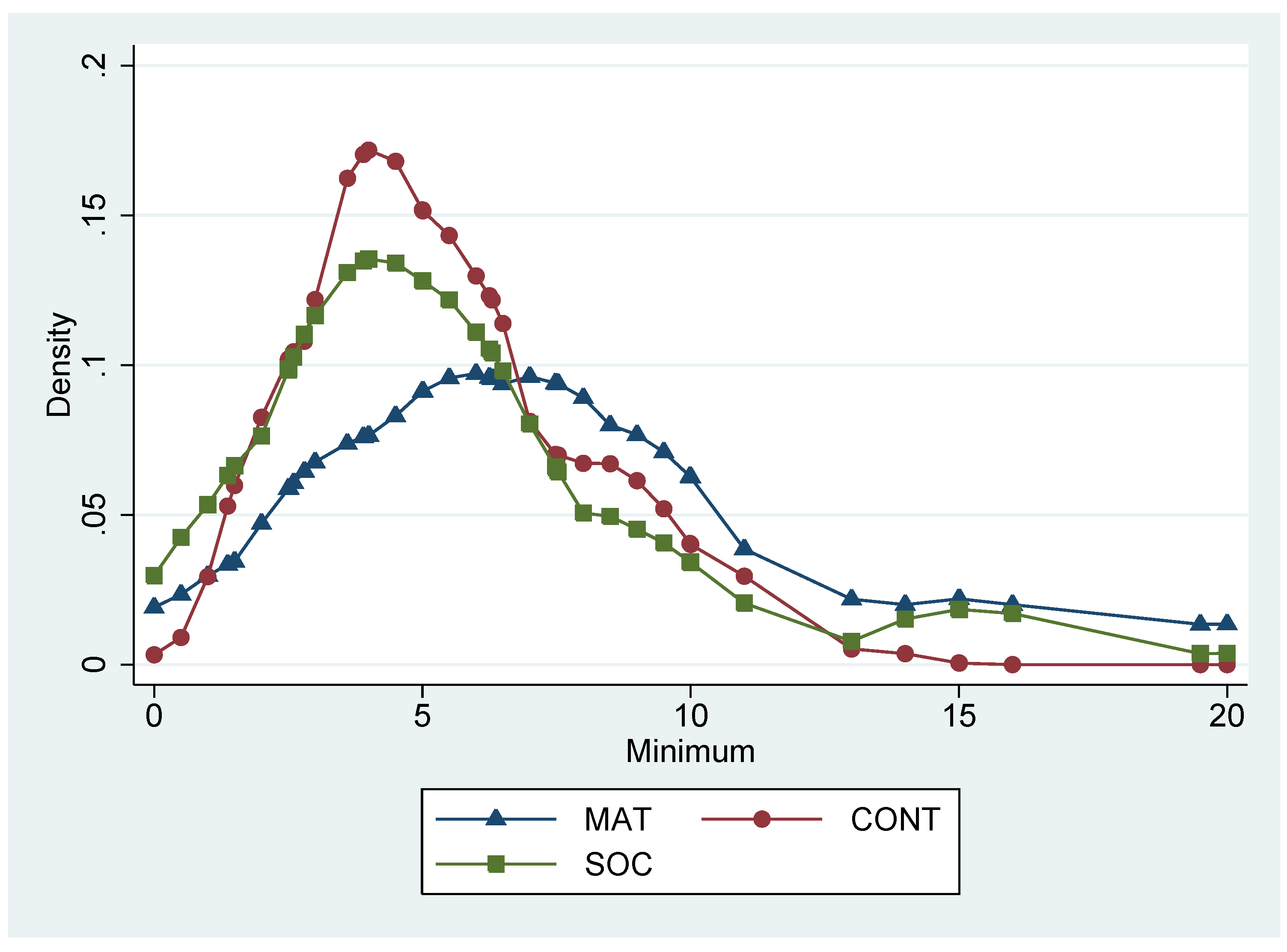
Figure 4.
Classroom experiment: Cumulative distribution of minimum over treatments.

Figure 5.
Classroom experiment: Distribution of risk premium over treatments.

Figure 6.
Classroom experiment: Cumulative distribution of risk premium over treatments.
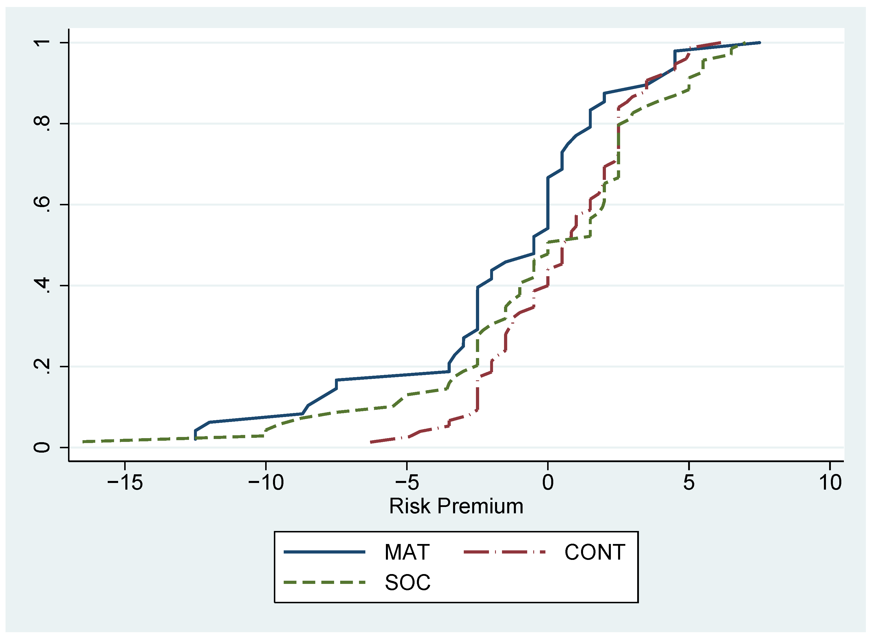
Figure 7.
Classroom experiment: Distribution of risk premium over treatments, scatter view. Horizontal differences between data points of one treatment are included for reasons of visibility.
Figure 7.
Classroom experiment: Distribution of risk premium over treatments, scatter view. Horizontal differences between data points of one treatment are included for reasons of visibility.
© 2010 by the author; licensee Molecular Diversity Preservation International, Basel, Switzerland. This article is an open-access article distributed under the terms and conditions of the Creative Commons Attribution license http://creativecommons.org/licenses/by/3.0/.
Share and Cite
MDPI and ACS Style
Matthey, A. The Influence of Priming on Reference States. Games 2010, 1, 34-52. https://doi.org/10.3390/g1010034
AMA Style
Matthey A. The Influence of Priming on Reference States. Games. 2010; 1(1):34-52. https://doi.org/10.3390/g1010034
Chicago/Turabian StyleMatthey, Astrid. 2010. "The Influence of Priming on Reference States" Games 1, no. 1: 34-52. https://doi.org/10.3390/g1010034