Modelling Social Dynamics (of Obesity) and Thresholds

Abstract

This paper focuses on the dynamic aspects of individual behavior affected by its social embedding, either at large (society-wide norms or averages) or at a local neighborhood. The emphasis is on how initial conditions can affect the long run outcome and to derive, discuss and apply the conditions for such thresholds. For this purpose, intertemporal social pressure (from peers, from norms, or from fashions) is modelled in two different ways: (i) individual benefit is influenced by the possession of a stock (in the application: weight) and the society wide average, and (ii) individual benefits depend on a norm that follows its own motion, of course driven by agents’ behavior. The topical issue of obesity serves as motivation and corresponding models and examples are presented and analyzed.

1. Introduction

The objective of this paper is to derive mechanisms linked to preferences affected by dynamic social interactions that allow for different long run outcomes contingent on initial conditions and in particular for threshold effects, i.e., starting above or below a threshold and thus at possibly similar initial conditions leads to different long run consequences. Further complexities such indeterminacy and limit cycles are addressed only in passing. The set up is a competitive symmetric equilibrium where agents lack strategic power. Therefore, the emphasis is on dynamics rather than on game theory, which is presumably complementary to most other contributions in this special issue.

The familiar but ‘easy’ route to history dependent outcomes—assuming increasing returns—is eschewed as well as the point in [1] that diminishing returns (rendering the first order conditions sufficient in contrast to easy route where the sufficient conditions are violated) allow for history dependence too. Instead history dependent outcomes are linked to different kinds of dynamic social interactions. For concreteness, these mechanisms and their potential explanatory power are applied to the topical issue of obesity by modelling the evolution of the body mass index (BMI). Dynamic mechanisms different from the ones in this paper are compiled in the book of [2].

The application to obesity is chosen for two reasons. Firstly, obesity is a dramatic yet very recent phenomenon in the industrialized countries in particular in the United States with some 20% of the population being obese (and even higher among blacks). Secondly, this phenomenon is often linked to social aspects, peer pressure and alike. One route to explain this dynamic phenomenon is that both a critical mass and social aspects (such as cultural ones consistent with the differences across ethnic groups) are crucial. For example, [3] uses dynamic simulations that relate the recent increases in obesity rates to falling food prices. [4] finds that self-control problems can explain the growth in BMI. Academic papers are however mixed on this issue, e.g., [5] questions the peer effect found in [6], and some papers argue that social pressure is in the form of discrimination, stigmatization and harassment and thus rather limiting than fostering obesity, e.g., [7].

Social interactions and social norms or benchmarks can affect individual preferences through different channels:

• The agent’s actions depend on the others’ (peers, averages, norms, law, etc.) actions. Since actions are a flow, corresponding social interactions are essentially static yielding a game of the type investigated first in [8] and later in many papers, e.g., in [9,10,11] that introduce moderate social influence as sufficient condition for unique outcomes in static social interaction games. More precisely, assume that the payoff of each player $\pi \left(b,B\right)$ depends on the own action, in our case the own body mass index (BMI) b, and on the average $\left(B\right)$, then moderate social influence (MSI), i.e.,

  $$\left|\frac{{\pi }_{bB}}{{\pi }_{bb}}\right|<1$$

  (1)

  is sufficient for a unique equilibrium of this static game. [12] applies the concept to quantify social multipliers.
• The agent’s preferences are affected by the relation of an individual stock, say wealth, education, weight, etc. vis a vis the same stock held by others. This requires a dynamic analysis, because the evolution of the stock, individually and aggregate, must be analyzed. This set up is considered in [6] in a fairly general form.
• Finally, the socially relevant variable is itself a dynamic process affected by the aggregate of private actions and stocks. In this case an additional differential equation traces the evolution of this ‘norm’, which is affected by the agent’s actions and stocks and which affects the individual preferences. For example how people like to dress will influence the evolution of fashions which in turn influences how people feel in their dress.

This paper focuses on dynamics and thus on the items 2 and 3. However, the last section proposes briefly a dynamic and also spatial extension departing from 1, i.e., static interactions. Section 2 investigates if the social reference level is itself a stock variable (say weight) and derives those conditions that are crucial for thresholds and relates them to a measure of dynamic social influence as a counterpart to (1); an application to obesity follows the theoretical exposition. Section 3 considers the consequences of norms that evolve on their own—some norms (good or bad) spread like a virus through the population. For example, most every day conventions concerning greeting, eating and recently smoking, removing dog droppings, etc.—moved slowly through the population, of course governed by the actions of members of the society and affecting their behavior; again this concept is first introduced in general and then applied to study the evolution of obesity. Section 4 considers briefly some extensions, first to more states and then to an entirely different framework (cellular automata) that requires less smart agents responding to observed behavior without the need (or even possibility) to forecast future social reference levels.

2. Social Reference Given by the Average Stock

2.1. Framework

The set up of agents’ intertemporal decisions concerning eating and their social interdependence follows the framework developed in [13]. More precisely, each agent solves the following optimal control problem of maximizing his net present value (using the constant discount rate $r>0$) of benefits subject to the the evolution of his weight,

$$\underset{\left\{e\right(t)\in \mathbb{R}\}}{max}\underset{0}{\stackrel{\infty }{\int }}exp\left(-rt\right)\pi \left(e\left(t\right)b\left(t\right),B\left(t\right)\right)dt$$

(2)

$$\dot{b}\left(t\right)=e\left(t\right),b\left(0\right)=b_0,b\left(t\right)\ge 0$$

(3)

$\pi (e,b,B)$ is the agent’s instantaneous benefit, ($\pi \in C^2$, jointly concave in $(e,b)$ and strictly in e), e is the control and describes the food intake (calories) in excess of metabolic needs, $b\left(t\right)$ is the agent’s body mass index in period t, which is assumed to be non-negative since we focus on obesity (we are not interested in anorexia nervosa, alternatively $b=0$ refers to the minimum weight). B is the average body mass index and in a symmetric equilibrium,

$$B\left(t\right)=b\left(t\right)\forall t$$

(4)

However, B is a datum given to individuals (if I acquire a large BMI $\left(b\right)$ then this has no effect on the, say Austrian, average). The appearance of B in the objective is crucial for the considered problem, because it matters how fat one is in comparison with the ‘others’, in particular, to attract sexual partners. At the same time, all what matters is that this average provides a benchmark in the sense of affecting individual payoffs, but not a norm in the normative sense, say like Kant’s categorical imperative (compare [14]). The differential equation traces the weight by accumulating consumption deviating from the level necessary to keep the weight unchanged, say $e_0$, which is assumed to be independent of the actual weight for reasons of simplicity only.

An equilibrium refers to a set of paths $\left\{e\left(t\right),b\left(t\right),B\left(t\right),t\in [0,\infty )\right\}$ that satisfy each agents’ optimality conditions and symmetry, $b\left(t\right)=B\left(t\right)$. A steady state of these equilibrium paths in the two-dimensional plane (due to the assumption of symmetry) can have one of the following (local) characteristics: unstable (the two eigenvalues of the Jacobian are positive or have positive real parts), which gives rise to thresholds (in particular if multiple steady states exist); saddlepoint stable (one eigenvalue is negative the other is positive) this gives (local) uniqueness since only the proper choice of the jumping variable (consumption, or equivalently the costate variable) allows to converge to the steady state; stable (both eigenvalues are negative or have negative real parts) which renders indeterminacy since any choice (thus uncountable many) allows to converge to the steady state.

Reference [13] shows that any (interior) steady state is characterized by the condition that the marginal rate of substitution between (over-) weight and eating must equal the discount rate,

$$\phi \left(b\right)\equiv -\frac{{\pi }_b\left(0,b,b\right)}{{\pi }_e\left(0,b,b\right)}=r$$

(5)

The existence of history dependent outcomes and related thresholds requires multiple steady states, one of them being unstable, i.e., the determinant of the Jacobian $\left(J\right)$ of the canonical equations induced by the first conditions of the maximization problem (2)-(4) must be positive. The following locally defined magnitude is crucial for dynamic behavior:

Definition: 

The expression,

$$DSI:=\left(-\frac{{\pi }_{bB}}{{\pi }_{bb}}\right)-\left(\frac{{\pi }_{eb}+{\pi }_{eB}}{{\pi }_{bb}}\right)r$$

(6)

is called the dynamic social influence (DSI), moderate if its (absolute) value is less than 1 and non-moderate if it is larger than 1.

This definition of dynamic social influence consists of three terms: social influence as measured in the static case (the first bracket in (6)) while the other two terms are dynamic in nature, because they reflect how the control (here eating) affects social interaction along the stock (weight in the application). Of these two terms, the term ${\pi }_{eb}$ is potentially void of social interactions such that $DSI\ne 0$ is possible without any social interaction (i.e., if B has no effect). Therefore, the definition of dynamic social influence extends the static counterpart and in fact, the property of moderate dynamic social influence (MDSI) is similar to MSI in static models, namely of ensuring stability and also that the slope of the stationary ‘reaction’ function is less than 1. Using this definition of dynamic social influence the following properties characterize thresholds (a sketch of the proof is given in the Appendix).

Positive and non-moderate dynamic social influence (NMDSI)

$$\left(-\frac{{\pi }_{bB}}{{\pi }_{bb}}\right)-\left(\frac{{\pi }_{eb}+{\pi }_{eB}}{{\pi }_{bb}}\right)r>1$$

(7)

is a necessary (but not sufficient) condition for a threshold. This condition implies locally evaluated at a steady state $\left(b_{\infty }\right)$ a negative determinant of the Jacobian and is equivalent to

$${\phi }^{\prime }\left(b_{\infty }\right)<0^1$$

(8)

A threshold (i.e., an unstable steady state) requires in addition

$$r>\frac{{\pi }_{eB}}{{\pi }_{ee}}$$

(9)

This condition holds trivially for the here plausible assumption of ${\pi }_{eB}\ge 0$, i.e., if the individual marginal utility from eating is increasing as the average BMI increases. For completeness, (7) coupled with the opposite inequality in (9) implies indeterminacy (i.e., stability of the steady state due to two negative eigenvalues of the Jacobian).

This proposition stresses that the static measure of social influence (1) is insufficient for the dynamic analysis, in particular, thresholds are possible if this static measure is moderate and the outcome can be unique even if this static measure is non-moderate. Of course, complementarity,

$${\pi }_{bB}>0$$

(10)

i.e., that the marginal ‘benefit’ from one’s own BMI is increasing if the average BMI is higher, is helpful for threshold effects. Indeterminacy requires at least, ${\pi }_{eB}<0$, i.e., marginal utility from consumption decreases as the average weight increases, which seems implausible in the context of obesity and such outcomes are thus ignored in the following.

2.2. Applications to Obesity

The following example departs from separable benefits and very simple functional forms (others like CRRA utility from consumption, exponential penalties for overweight, etc. will do the same) and parameterization. Payoff π consists of: utility from eating—assuming the most simple linear-quadratic utility from eating beyond the metabolic needs, $u=e-\frac{e^2}{2}$—minus the corresponding expenditures $\left(pe\right)$ where p denotes the price per unit of food and the constant expenditures for meeting the metabolic needs are ignored because they are irrelevant for the optimization; the utility loss from over-weight $\left(k>0\right)$; the loss (or benefit) from one’s body shape relative to the average ($v>0$, this delivers the crucial complementarity, ${\pi }_{bB}>0$); and two dynamic interaction terms that are helpful to establish NMDSI,

$$\pi \left(e,b,B\right)=e-\frac{e^2}{2}-pe-\frac{k}{3}{b}^3-v\frac{b}{B}+\alpha eb+\beta eB$$

(11)

The first, ${\pi }_{eb}=\alpha >0$ accounts for addictive elements of eating, or for a gourmet aspect, because a rich history of eating may provide a better evaluation and joy from eating compared with people just meting their metabolic needs $\left(b=0\right)$. The second interaction term, ${\pi }_{ex}=\beta >0$, is social from the beginning (and not only indirectly as the first one) and captures that one can enjoy eating more if all relevant people are over-weight too, e.g., by mitigating otherwise bad conscience. The corresponding derivatives,

$$\begin{array}{ccc}\hfill {\pi }_e& =& 1-e-p,{\pi }_{ee}=-1<0,{\pi }_{eb}=\alpha >0,{\pi }_{eB}=\beta >0\hfill \\ \hfill {\pi }_b& =& -k{b}^2-\frac{v}{B},{\pi }_{bb}=-2kb,{\pi }_{bB}=\frac{vb}{B^2}\hfill \\ \hfill {\pi }_B& =& \frac{vb}{B^2}=\frac{v}{b}\text{at}\text{a}\text{symmetric}\text{equilibrium}\hfill \end{array}$$

imply complementarity and that the agent’s objective is jointly concave in the individual variables if the corresponding determinant of the Hessian is positive,

$${\pi }_{ee}{\pi }_{bb}-{\pi }_{eb}^2=2vb-{\alpha }^2>0$$

(12)

which is the case for $b>\frac{{\alpha }^2}{2v}$. Non-moderate dynamic social influence is necessary for any kind of complexity and the corresponding crucial condition for NMDSI (or $det\left(J\right)>0$ or respectively ${\phi }^{\prime }<0$) is,

$$\left(\alpha +\beta \right)r+\frac{v}{y^2}-2ky>0$$

(13)

which holds at ‘low’ levels of steady states as candidates for thresholds (indeterminacy can be ruled out since ${\pi }_{eb}>0$), while the opposite inequality and thus saddlepoint stability applies to larger steady states, of course provided that multiple steady states exist. This calculation stresses how different kinds of interactions contribute to non-moderate dynamic social influence and thus to complexity: social interaction as in the static games, ${\pi }_{bB}>0$, which is here related to the sign (positive, i.e., complementary) and size of the parameter v, and the inherently dynamic interaction terms ${\pi }_{eB}=\alpha$ and also ${\pi }_{eb}=\beta$, which has no obvious social link. Indeed one can find examples for thresholds even if the static interaction is moderate or entirely missing (e.g., in the wealth example below).

Using the above derivatives and the symmetry (4) in the corresponding first order conditions yields the canonical equations,

$$\begin{array}{ccc}\hfill \dot{b}& =& 1+\mathsf{\lambda }-p+\left(\alpha +\beta \right)b\hfill \end{array}$$

(14)

$$\begin{array}{ccc}\hfill \dot{\mathsf{\lambda }}& =& \left(r-\alpha \right)\mathsf{\lambda }-\alpha \left(1-p+\left(\alpha +\beta \right)b\right)+\frac{v}{b}+k{b}^2\hfill \end{array}$$

(15)

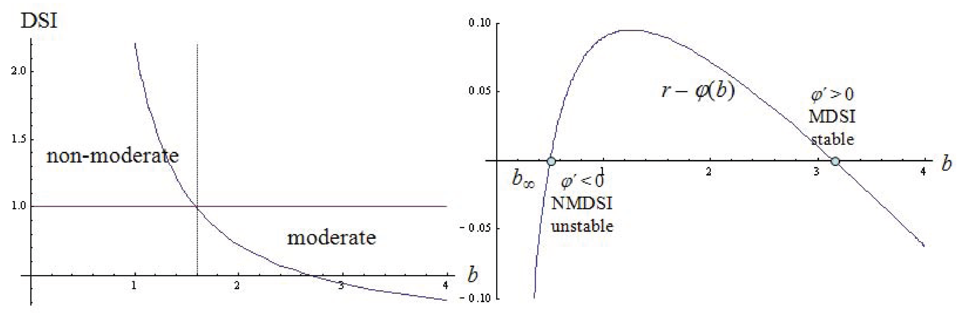
where the right hand side of $\dot{b}$ is the optimal consumption rule after substituting (4). Figure 1 uses a particular numerical example of (11) to demonstrate the construction of the crucial elements without any need to solve (at this exploratory stage) the canonical equations or to compute the steady states. It plots on the left hand side the magnitude of dynamic social influence (DSI) and on the right hand side the steady state condition,

$$r-\phi \left(b\right)=r-\frac{v+k{b}^3}{b\left(1-p+\left(\alpha +\beta \right)b\right)}=0$$

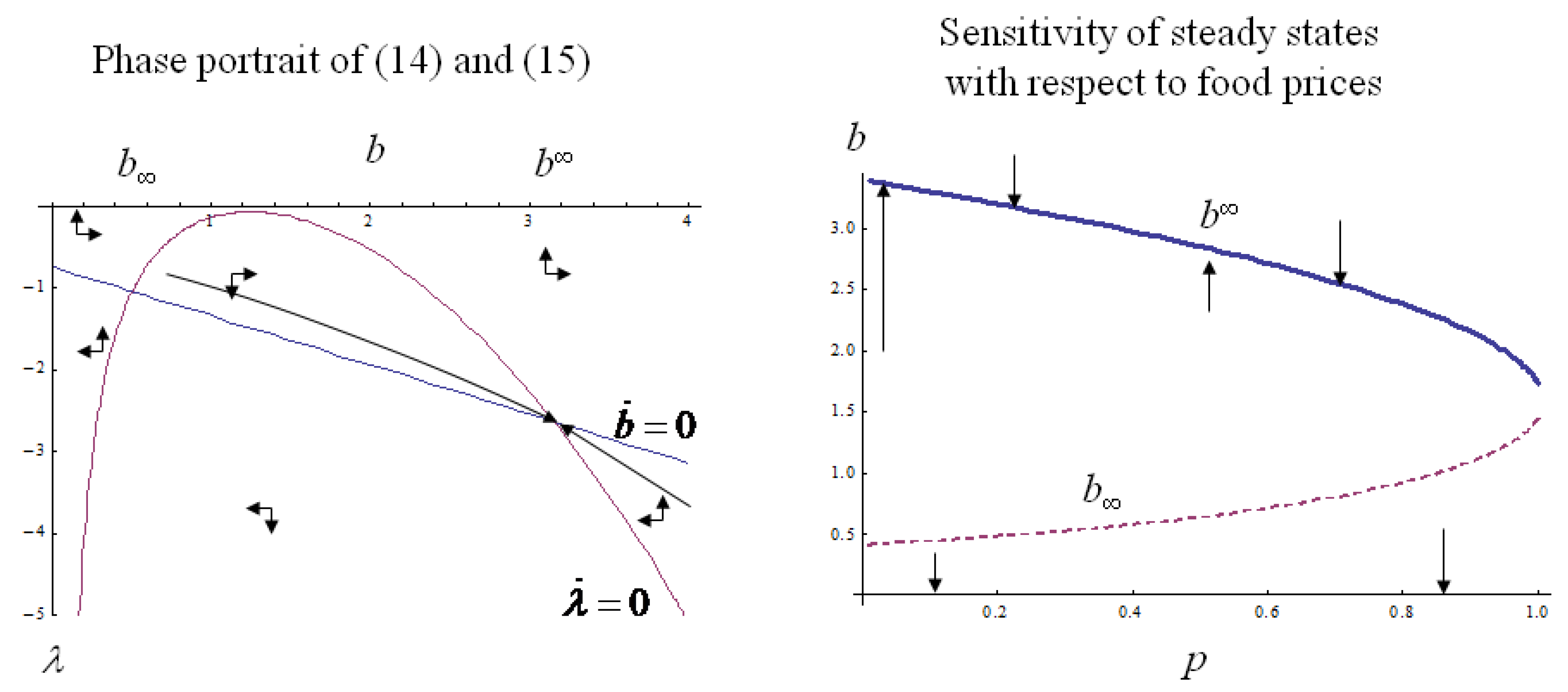
which yields two steady states in the (relevant) positive orthant that satisfy the state constraint (there exists a third root for $b<0$). The lower steady state, $b_{\infty }$ (payoff is jointly concave there), is in the domain of NMDSI. This follows also from ${\phi }^{\prime }\left(b_{\infty }\right)>0$, which in turn implies instability (Proposition 1), because the real parts (of the two complex) eigenvalues of the Jacobian $\left(J\right)$ of the above system of differential equations (14)–(15) are positive. The second steady state $b^{\infty }$ is a saddlepoint $\left(det\left(J\right)<0\right)$ due to ${\phi }^{\prime }\left(b^{\infty }\right)>0$. Hence the long run outcome will be either a society with a high BMI (the saddlepoint stable interior steady state) or the boundary solution $b\to 0$ (no over-weight). However, the long run outcome depends here not only on the initial condition but also on expectations. The reason is that the lower steady state is an unstable focus (both eigenvalues are complex) as indicated in the phase portrait on the left hand side of Figure 2, which creates an overlap. i.e., an interval of initial conditions $b_0\in \left(\underline{b},\overline{b}\right)$ that all allow to reach the two (saddlepoint) stable steady states (0 and $b^{\infty }$ in Figure 3) by satisfying all optimality and consistency conditions, compare [15] and [13] for computing this overlap. In such a case, history (i.e., an initial condition) is insufficient to determine the long run outcome and assumptions about the agents’ expectations beyond assuming rational expectations are necessary to determine the economy’s evolution.

Reference [16] relates obesity to the fall in food prices. A related result (the negative dependence of the stable long run outcome on food prices seems obvious) can be also established with respect to the threshold. The right hand side of Figure 2 shows the steady states for different food prices $\left(p\right)$ and how the lower steady state and thus the threshold (as mentioned, there exist overlaps around this lower steady state) increases with respect the food price. Therefore, an exogenous lowering of food prices can turn society away from its move towards normal weight (say in Europe after the eating binge following the second world war) to a path heading towards the obese steady state.

Figure 1. Dynamic social influence (DSI) and determination of steady states for the example (11) and the parameter values: $r=0.2,p=0.25,\alpha =0.1,\beta =\frac{1}{2},k=0.05,v=0.1.$

Figure 1. Dynamic social influence (DSI) and determination of steady states for the example (11) and the parameter values: $r=0.2,p=0.25,\alpha =0.1,\beta =\frac{1}{2},k=0.05,v=0.1.$

Figure 2. Example of specification (11) for the parameter values: $r=0.2,p=0.25,\alpha =0.1,\beta =\frac{1}{2},k=0.05,v=0.1.$

Figure 2. Example of specification (11) for the parameter values: $r=0.2,p=0.25,\alpha =0.1,\beta =\frac{1}{2},k=0.05,v=0.1.$

2.3. Other Applications

2.3.1. Labor Market

Workers move at a rate $\dot{y}=u$ incurring quadratic costs between ‘agriculture’ ${}_a$ and ‘manufacturing’ ${}_m$ that pays higher wages if sufficiently many work in factories (due to the increasing returns in manufacturing). An individual worker’s instantaneous payoff is

$$\pi (x,y,u)=y{w}_m\left(x\right)+\left(1-y\right)w_a-\frac{k}{2}{u}^2$$

(16)

where $w_a$ and $w_m$ are the wages. Wages in agriculture $\left(w_a\right)$ are constant, while the wages in manufacturing depend positively (due to increasing returns) on the degree of industrialization, i.e., on the average time that all workers spend in factories (denoted by x), $w_m\left(\tilde{x}\right)=w_a$, $w_m^{\prime }>0$, $w_m^{\prime \prime }=0$, where $\tilde{x}=$ critical level at which manufacturing pays the same wage as agriculture. The variable $0\le y\le 1$ is the individual time spent in the factory, thus $\left(1-y\right)$ is the time the agent works in the fields. [15] emphasizes that externalities and increasing returns, a theme trumped by Brian Arthur in many ways, e.g., in [17], are necessary for multiple equilibria in this and other frameworks. However, [18] shows that increasing returns are neither necessary nor sufficient and that it is non-moderate social influence (i.e., the opposite inequality in (1))) coupled with complementarity (10) that triggers multiple long run outcomes considering the generalization $w\left(y,x\right)$ for the earnings in manufacturing (the multiplicative term in (16) implies increasing returns in manufacturing).

2.3.2. Wealth Status

Reference [19] extends the standard open-economy Ramsey model by accounting for wealth related status (in passing it shows that the consideration of status is observational equivalent to benefit from wealth in spite of the externality induced by status considerations): Agents’ benefits consist of neoclassical utility from consumption $u\left(c\right)$ and status s depending on own $\left(a\right)$ and average $\left(A\right)$ wealth subject to the evolution of assets a, (earning constant interest $\rho <r$ and a constant wage w) and a no-Ponzi game condition:

$$\begin{array}{ccc}& & \underset{\left\{c\right(t\left)\right\}}{max}\underset{0}{\overset{\infty }{\int }}exp(-rt)\left[u\left(c\right)+s(a,A)\right]dt\hfill \end{array}$$

(17)

$$\begin{array}{ccc}\hfill \dot{a}& =& \rho a+w-c,a\left(0\right)=a_0,\underset{t\to \infty }{lim}a\left(t\right)e^{-\rho t}\ge 0\hfill \end{array}$$

(18)

First of all transforming (17) and (18) into the set up (2)—(4), $\rho a+w-c\to e$, results in the payoff

$$\pi \left(e,a,A\right)=u(\rho a+w-e)+s(a,A)$$

It is very simple to obtain history dependent outcomes (almost generic if an interior steady state exists), which in addition eliminates the (implausible) boundary outcome in the standard model, $y\to -w/\rho$, $e\to 0$, [20], but only conditional on not too much debt at the beginning.

2.3.3. Addiction

Adding social interactions to the rational addiction model of [21] yields,

$$\begin{array}{ccc}& & \underset{\left\{c\right(t\left)\right\}}{max}\underset{0}{\stackrel{\infty }{\int }}exp(-rt)\left[u(c,y,x)-pc\right]dt\hfill \end{array}$$

(19)

$$\begin{array}{ccc}\hfill \dot{y}& =& c-\delta y,y\left(0\right)=y_0\hfill \end{array}$$

(20)

in which c is current drug consumption, y measures the history of drug use (δ is the corresponding depreciation rate), and $u_{cy}>0$ captures addiction: a higher level of addiction as measured by y causes a higher loss in marginal utility from a reduction in consumption. This sign is similar to the above modelling of obesity, which contains therefore an element of addiction if the utility loss from dieting increases (at the margin) with respect to one’s overweight. Already [21] addresses the issue of history dependence but relates that to the non-concavity of utility with respect to the state, which is the well known route to thresholds that is not pursued in this paper. Instead introducing the corresponding aggregate of addiction prevalent within the relevant group, denoted by x and $x=y$ in a symmetric equilibrium, accounts for peer or social pressure. Given this influence and complementarity (presumably related to peer group rather than the population at large) one can trigger different long run outcomes conditional on initial conditions similar to the above example about obesity.

2.3.4. Fashions

Agents have preferences for certain kinds of clothes (e.g., a short or a long skirt) and at the same time want to follow a fashion, or want to distance themselves from a trend. Thus let x denote the average or aggregate of ‘in’-dresses and y the corresponding private possessions and $p(x,y)$ the individual benefit to show off with y given that the others own $x.$ Accounting for the costs, $k\left(c\right)$, positive for acquiring c pieces ($k^{\prime }>0$ for $c\ge 0$) and zero or negative (i.e., for a price paid in the second hand market) for getting rid of a piece results in an asymmetry due to imperfections of the second hand market.

3. Model II—Dynamic Social Norms

The model is as in (2) and (3) but with the difference that the social norm is not equal to the average but is itself the outcome of a dynamic process. For example, a fashion created by a particular event (movie), new role models (e.g., anorectic models, like Twiggy in 1960s), etc. create a benchmark, which itself feeds on the public acceptance and this acceptance in turn determines the future benchmark. For example, famous people can (and have) made drug abuse popular and as the drug abuse increases, the social stigma with drug use may increase or decrease. Or on the positive side, the behavior of famous people such as movie and rock stars buying organic food, fair-trade products, hybrid cars, and offsets for carbon emissions (e.g., the Rolling Stones on their last World Tour) may set a new norm as, e.g., the enormous increase of the revenues of fair-trade goods even during the recession year 2009 documents (more precisely2, by 11.9% for bananas with a share of already 32.5%). Such norms may spread like a virus through the population.

Using the notation from above and introducing a general set up, N denotes the current norm or reference point for individuals affecting their payoffs where the conceivable dependence on the aggregate B is dropped in order to focus on the separate and dynamic evolution of the norm,

$$\pi =\pi \left(e,b,N\right)$$

The norm evolves contingent on social aggregates (individuals have again measure zero) including E for average consumption (static spillovers in π are ignored, i.e., no E appears in π),

$$\dot{N}=g\left(E,B,N\right)$$

Reference [22] considers such dynamic externalities in pure adjustment cost models proving existence and deriving conditions for limit cycles ($g_N>0$ at a steady states fosters a bifurcation for sufficiently convex adjustment costs, while $g_N<0$ ensures saddlepoint stability); [23] considers the general system (derived below) but focuses also on limit cycles.

Given this additional state, the first order conditions do not change except for the additional dependence of the control (here consumption e) on the norm N, thus

$$\begin{array}{ccc}\hfill e^{*}& =& e^{*}\left(b,\mathsf{\lambda },N\right)\hfill \\ \hfill e_b^{*}& =& -\frac{{\pi }_{eb}}{{\pi }_{ee}},e_{\mathsf{\lambda }}^{*}=-\frac{1}{{\pi }_{ee}},e_N^{*}=-\frac{{\pi }_{eN}}{{\pi }_{ee}}\hfill \end{array}$$

Assuming that the agents have rational expectations, i.e., perfect foresight of the future norms in this deterministic framework, the following triple of differential equations characterizes a symmetric perfect foresight equilibrium,

$$\begin{array}{ccc}\hfill \dot{b}& =& e^{*}\left(b,b,N,\mathsf{\lambda }\right),b\left(0\right)=b_0\hfill \end{array}$$

(21)

$$\begin{array}{ccc}\hfill \dot{\mathsf{\lambda }}& =& r\mathsf{\lambda }-{\pi }_b\left(e^{*}\left(b,b,N,\mathsf{\lambda }\right),b,b,N\right),\underset{t\to \infty }{lim}exp\left(-rt\right)b\left(t\right)\mathsf{\lambda }\left(t\right)=0\hfill \end{array}$$

(22)

$$\begin{array}{ccc}\hfill \dot{N}& =& g(e^{*}\left(b,b,N,\mathsf{\lambda }\right),b,N),N\left(0\right)=N_0\hfill \end{array}$$

(23)

The eigenvalues of the Jacobian J of the above differential equation system,

$$\begin{array}{ccc}\hfill J& =& \left(\begin{array}{ccc}{e}_b^{*}& e_{\mathsf{\lambda }}^{*}& e_N^{*}\\ -{\pi }_{be}{e}_b^{*}-{\pi }_{bb}& r-{\pi }_{be}{e}_{\mathsf{\lambda }}^{*}& -{\pi }_{be}{e}_N^{*}-{\pi }_{bN}\\ g_e{e}_b^{*}& g_e{e}_{\mathsf{\lambda }}^{*}& g_e{e}_N^{*}+g_N\end{array}\right)\hfill \\ & =& -\frac{1}{{\pi }_{ee}}\left(\begin{array}{ccc}{\pi }_{eb}& 1& {\pi }_{eN}\\ {\pi }_{ee}{\pi }_{bb}-{\pi }_{eb}^2& -\left(r{\pi }_{ee}+{\pi }_{be}\right)& {\pi }_{bN}{\pi }_{ee}-{\pi }_{be}{\pi }_{eN}\\ g_e{\pi }_{eb}& g_e& g_e{\pi }_{eN}-g_N{\pi }_{ee}\end{array}\right)\hfill \end{array}$$

(24)

determine the local stability properties of a hyperbolic system and they are given by the roots of the characteristic polynomial,

$$\begin{array}{ccc}\hfill P\left(\epsilon \right)& =& {\epsilon }^3-\text{tr}\left(J\right){\epsilon }^2+\omega \epsilon -det\left(J\right)\hfill \end{array}$$

(25)

$$\begin{array}{ccc}\hfill \text{tr}\left(J\right)& =& r+g_N-\frac{{\pi }_{eN}}{{\pi }_{ee}}{g}_e,\hfill \end{array}$$

(26)

$$\begin{array}{ccc}\hfill \omega & =& \frac{{\pi }_{eB}{g}_B-{\pi }_{bb}+r\left({\pi }_{ee}{g}_N-{\pi }_{eb}\right)}{{\pi }_{ee}}\hfill \\ & & +\frac{g_e\left({\pi }_{eB}\left({\pi }_{eB}-{\pi }_{eb}\right)-{\pi }_{ee}\left({\pi }_{bB}+r{\pi }_{ee}\right)\right)}{{\pi }_{ee}^2}\hfill \end{array}$$

(27)

$$\begin{array}{ccc}\hfill det\left(J\right)& =& \frac{g_B{\pi }_{eB}\left({\pi }_{eb}-{\pi }_{eB}\right)}{{\pi }_{ee}^2}+\frac{\left(r+{\pi }_{bB}\right)g_B-\left({\pi }_{bb}+r{\pi }_{eb}\right)g_N}{{\pi }_{ee}}\hfill \end{array}$$

(28)

The three eigenvalues $\{{\epsilon }_1,{\epsilon }_2,{\epsilon }_3\}$ can be explicitly calculated and vice versa these eigenvalues ${\epsilon }_i$ determine the coefficients (26)–(28) of the characteristic polynomial, see Table 1. Given this three-dimensional system, usual saddlepoint stability implies for each initial condition $\left(b_0,N_0\right)$ a unique initial value of the costate ${\mathsf{\lambda }}_0$. The associated two-dimensional stable manifold in the $\left(b,\mathsf{\lambda },N\right)$—space corresponds to the case where two eigenvalues have negative real parts (or are negative). In contrast, thresholds require that the stable manifold is one-dimensional (one eigenvalue is negative, the other two are positive or have positive real parts). The projection of this manifold into the $\left(b,N\right)$-space is a line that separates the basins of attractions of the (saddlepoint-) stable steady states and as in the simpler framework of Section 2 there may exist also an overlap. Finally, if all eigenvalues are negative or have negative real parts, indeterminacy results, because irrespective where we start (of course sufficiently close to a steady state due to the local nature of the analysis), we will converge to steady state. The following two propositions, which are taken from and proven in [23], summarize the different outcomes.

Table 1. Relation between eigenvalues the coefficients of (25).

assuming ${\epsilon }_3\in \mathbb{R}$
	$\begin{array}{c}{\epsilon }_{1,2}\in \mathbb{R}\hfill \end{array}$	$\begin{array}{c}{\epsilon }_{1,2}=\rho \pm \omega i\hfill \end{array}$
$\begin{array}{c}\hfill det\left(J\right)=\end{array}$	$\begin{array}{c}{\epsilon }_1{\epsilon }_2{\epsilon }_3\end{array}$	$\begin{array}{c}{\epsilon }_3({\rho }^2+{\omega }^2)\hfill \end{array}$
$\begin{array}{c}\hfill tr\left(J\right)=\end{array}$	$\begin{array}{c}{\epsilon }_1+{\epsilon }_2+{\epsilon }_3\end{array}$	$\begin{array}{c}{\epsilon }_3+2\rho \hfill \end{array}$
$\begin{array}{c}\hfill \omega =\end{array}$	$\begin{array}{c}{\epsilon }_1({\epsilon }_2+{\epsilon }_3)+{\epsilon }_2{\epsilon }_3\end{array}$	$\begin{array}{c}2\rho {\epsilon }_3+({\rho }^2+{\omega }^2)\hfill \end{array}$
Source: [23].

Table 1. Relation between eigenvalues the coefficients of (25).

assuming ${\epsilon }_3\in \mathbb{R}$
	$\begin{array}{c}{\epsilon }_{1,2}\in \mathbb{R}\hfill \end{array}$	$\begin{array}{c}{\epsilon }_{1,2}=\rho \pm \omega i\hfill \end{array}$
$\begin{array}{c}\hfill det\left(J\right)=\end{array}$	$\begin{array}{c}{\epsilon }_1{\epsilon }_2{\epsilon }_3\end{array}$	$\begin{array}{c}{\epsilon }_3({\rho }^2+{\omega }^2)\hfill \end{array}$
$\begin{array}{c}\hfill tr\left(J\right)=\end{array}$	$\begin{array}{c}{\epsilon }_1+{\epsilon }_2+{\epsilon }_3\end{array}$	$\begin{array}{c}{\epsilon }_3+2\rho \hfill \end{array}$
$\begin{array}{c}\hfill \omega =\end{array}$	$\begin{array}{c}{\epsilon }_1({\epsilon }_2+{\epsilon }_3)+{\epsilon }_2{\epsilon }_3\end{array}$	$\begin{array}{c}2\rho {\epsilon }_3+({\rho }^2+{\omega }^2)\hfill \end{array}$
Source: [23].

Assume that $det\left(J\right)>0$ at a steady state, then the following stability properties hold:

• Either $tr\left(J\right)<0$ or $\omega <0$ saddlepoint stability, i.e., two eigenvalues are either negative or have negative real parts.
• A pair of complex eigenvalues with non-negative real parts, thus local instability $tr\left(J\right)>0$ and $\omega >0$; yet the converse does not hold, i.e., $det\left(J\right)>0$, $tr\left(J\right)>0$ and $\omega >0$ still allow for saddlepoint stability.
• $det\left(J\right)=tr\left(J\right)\omega$ (where $tr\left(J\right)>0$ and $\omega >0$) leads to a pair of purely imaginary eigenvalues. Possibly associated with this ‘bifurcation’ are limit cycles. In fact, stable limit cycles exist.

Assume that $det\left(J\right)<0$ at a steady state, then the following stability properties hold

• $det\left(J\right)<tr\left(J\right)\omega$ implies instability, i.e., only one eigenvalue is negative, the other two are positive or have positive real parts.
• Total stability, i.e., all eigenvalues are negative or have negative real parts iff $tr\left(J\right)<0,\omega >0,det\left(J\right)<0$ and $det\left(J\right)>tr\left(J\right)\omega$.

The crucial point is again to find multiple equilibria of which one must be unstable in order to give rise to a threshold, case one in the above Proposition 3. Derivation of general conditions that are comparable to those in the previous section are much more cumbersome and thus the remainder of this section focuses on an example.

3.1. Application to Obesity

The importance of social norms and of their dynamic evolution is stressed in [16]: “in 1994, average weight for an American woman was 147 pounds, and the average desired weight was 132 pounds. By 2002, the average had increased to 153 pounds, and average desired weight had increased to 135 pounds. These figures ... suggest a reduction in ... social pressure to maintain lower weights. The recent survey of weight perception finds that 87% of Americans, including 48% of obese Americans, believe that their body weight falls in the “socially acceptable” range.” A simple example how facts adjust norms dynamically (as suggested by the above quote) is

$$\dot{N}=N\left(1+B-N\right)$$

(29)

In words, $N=1$ is something like the natural norm given, which corresponds to $B=0$ and all having a perfect BMI. However, as the overweight in the society increases the norm adjusts upwards and at a steady state, $N_{\infty }=B_{\infty }+1$. The dynamic rise in the norm follows in (29) the familiar logistic law. Eliminating all other kinds of social interactions in order to focus on this dynamically evolving norm (and of course to simplify) and to differentiate the specification from the one in (11), consider the following simple payoff for an individual,

$$\pi \left(e,b,N\right)=ln\left(e_{min}+e\right)-pe-\frac{k}{2}{b}^2-v{\left(\frac{b+1}{N}\right)}^2$$

(30)

where $e_{min}$= the metabolic need, $\left(pe\right)$ are the food expenditures (the constant expenditure $p{e}_{min}$ have no effect on the intertemporal optimization), and quadratic penalties for overweight (and thus as well as for anorectic BMIs) and for deviating from the norm. This implies the following characterization of a dynamic, symmetric competitive equilibrium,

$$\begin{array}{ccc}\hfill \dot{b}& =& \frac{1+e_{min}\left(\mathsf{\lambda }-p\right)}{p-\mathsf{\lambda }}\hfill \end{array}$$

(31)

$$\begin{array}{ccc}\hfill \dot{\mathsf{\lambda }}& =& r\mathsf{\lambda }+kb+\frac{2v\left(1+b\right)}{N^2}\hfill \end{array}$$

(32)

$$\begin{array}{ccc}\hfill \dot{N}& =& N\left(1+b-N\right)\hfill \end{array}$$

(33)

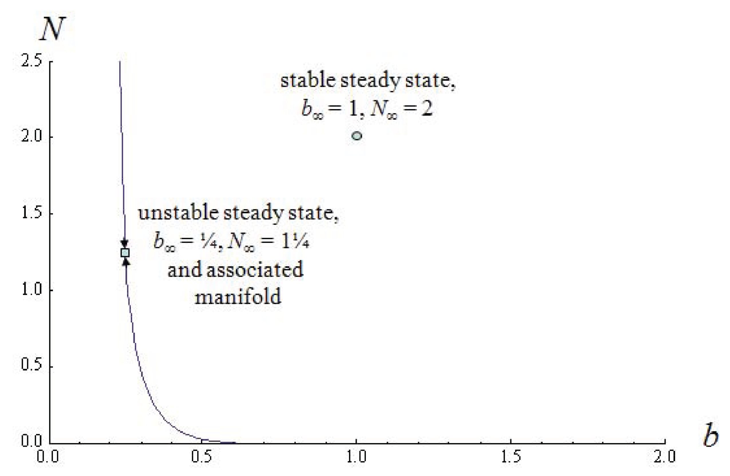
This example permits the computation the coefficients of the characteristic polynomial and of the (two) steady states (suppressed but available on request) of which the lower steady state (if existing and identified by subscripted ∞ in Figure 3) is unstable and a node creating a threshold in the space of state $\left(b\right)$ and the norm $\left(N\right)$. Figure 3 shows these steady states and constructs (numerically) the one-dimensional manifold in the state space separating the domains of attractions where to the left of this threshold, the system converges to the boundary equilibrium determined by the state constraint, $b\ge 0$, i.e., normal BMI. Variations in food prices $\left(p\right)$ have an effect very similar to one shown in Figure 2.

Figure 3. Multiple steady states and intertemporal equilibria due to (dynamic) norms of the example (30) and the parameter values: $r=0.5,e_{\text{min}}=0.1,p=1,k=2,v=2.5.$

Figure 3. Multiple steady states and intertemporal equilibria due to (dynamic) norms of the example (30) and the parameter values: $r=0.5,e_{\text{min}}=0.1,p=1,k=2,v=2.5.$

4. Extensions

4.1. Additional (Private) States

Clearly, introducing a second state $\left(x\right)$ into (2)–(4) allows for further realism and does not complicate the analysis much beyond the one in the previous section: the optimal motions take place in a two-dimensional manifold in a four-dimensional space (if ignoring now the aspects of dynamic social norms) such that the threshold is a curve in the state space and that limit cycles are possible, as in the case of a dynamic norm. Some examples relevant for the case of obesity follow.

Gourmet

One may add another stock of consumption history,

$$\dot{x}=f\left(e,x\right)=e-\theta x$$

that accounts for the second effect from eating in building up a taste (as already briefly mentioned); θ describes how this taste depreciates. This stock (taste) increases the (marginal) benefit from eating $\left({\pi }_{ex}>0\right)$, e.g., by avoiding low quality food, may have direct benefit from one’s self image of being a connoisseur (of wine, or food, thus, ${\pi }_x>0$) and such a reputation of being a gourmet can provide in addition an element of social status, ${\pi }_{xX}>0$. [24] considers a related two state variable model of (drug) consumption without social interactions and show that strictly concave preferences permit limit cycles given sufficient ‘adjacent complementarity’, [25].

Wealth

Another alternative is to include wealth $\left(a\right)$ as expressed in (18) but where it makes sense to assume that the wage depends on aggregate and individual BMI, $w=w\left(b,B\right)$. In addition own wealth matters directly and/or including a social element, i.e., relative to average wealth. [26] shows that the inclusion of such wealth effects (again without social interactions) allows for limit cycles in a model of rational addiction even for separable specifications and thus for a different reason than in [25].

4.2. Cellular Automata

Finally, we address also the first channel mentioned in the introduction and consider static preferences and social interactions but within a dynamic and also spatial framework. Including simultaneously time and space in the investigation amounts to study partial differential equations, which are hard to analyze and are therefore hardly applied in economics. Therefore, cellular automata are proposed, which provide a simple framework allowing for rich outcomes, see [27,28] for an exposition, even a new kind of science according to [29]. To some surprise, economic applications of this powerful instrument are rare and a few exceptions are [30] on conventions and [31] on bureaucratic corruption.

With static preferences, an agent’s payoff depends on own action and those of the relevant group. The relevant group consists of ‘neighbors’, for simplicity with radius r in a linear city along a circle (in the two-dimensional case one has to differentiate between different—von Neumann or Moore—neighborhoods). Given the complex interactions of these overlapping neighborhoods rational expectations are impossible (at least in general, in particular if the automaton is of class 3 or even of class 4, see [27,28] for corresponding definitions); compare also the related example about visiting the El-Farol bar [32]. Therefore, agents must act myopically ([3] makes a similar assumption) observing the past behavior of their neighbors, when they maximize their own payoff (identical for each agent in our symmetric set up),

$$\underset{b_{it}}{max}\pi \left(b_{it},b_{i-r,t-1},...,b_{i-1,t-1},b_{it-1},b_{i+1,t-1},...,b_{i+r,t-1}\right)$$

Applying the implicit function theorem (assuming, ${\pi }_{b_{it}^2}<0$) to the above maximization implies a map of the observed past actions into the new action,

$$b_{it}^{*}=F\left(b_{it},b_{i-r,t-1},...,b_{i-1,t-1},b_{i,t-1},b_{i+1,t-1},...,b_{i+r,t-1}\right)$$

A cellular automaton is an iterating map F—above (and in economics in general) described by the individual agent’s maximization—that updates in each period t the action of a site i, here $b_{it}$, depending on the neighbors’ actions in period $(t-1)$ from a fixed radius r into the set of feasible actions. The action space is typically discrete and of dimension k, $b_{it}\in \left\{0,1,...k-1\right\}$. Individual payoffs depend on the current action $\left(u\right)$ and how this action compares with those of the neighbors $\left(v\right)$. For reasons of simplicity only the aggregate over the past actions in the neighborhood matters $\left(B_{i,t-1}\right)$,

$$b_{it}=F\left(B_{i,t-1}\right):=\underset{b_{it}\in \left\{0,1,...k\right\}}{max}\pi \left(b_{it},B_{i,t-1}\right)=u\left(b_{it}\right)+v\left(b_{it},B_{i,t-1}\right)$$

(34)

$$B_{i,t-1}=\underset{j=-r}{\sum ^r}{b}_{i+j,t-1}\text{or}{B}_{i,t-1}=\underset{j=-r}{\sum ^{-1}}{b}_{i+j,t-1}+\underset{j=1}{\sum ^r}{b}_{i+j,t-1}$$

(35)

The first definition of $B_{i,t-1}$ includes the own past action and is called totalistic, while the second definition considers only the neighbors and is called outer-totalistic. Therefore, all what is needed is a decision rule, here for all possible constellations of $B_{i,t-1}$, which gives ${\left(2r\right)}^{k-1}$ combinations for the first definition of $B_{i,t-1}$.

In the context of obesity think that during winter-time, eating provides benefit to ease winter depression $u\left(b_{it}\right)$ but the corresponding gain in weight will put one at a disadvantage in the summer season (shorts or bikinis depending on gender) if one’s neighbors ate less. Self-images of the agent (compare [33]), health concerns etc. may induce additional costs on overeating, which all are part of $v\left(b_{it},B_{i,t-1}\right)$. Of course, the more of your peers are slim, the more harmful is one’s overweight. For a start consider two actions: to enter the season normal $\left(0\right)$, or obese $\left(1\right)$ and a radius of $r=3$. The first action entails private costs but social gains and the converse holds for the second option, eating, where the benefit from eating may depend on the observed state: being obese among slim friends may generate a bad conscience from eating. As mentioned, restriction to totalistic rules allows for different outcomes from 0 up to 7 if the own past actions have an influence too. Figure 3 shows the outcome for the simple rule that individual behavior simply follows the majority (rule $\#240=2^7+2^6+2^5+2^4$),

$$b_{it}=\left\{\begin{array}{c}1\\ \\ 0\end{array}\text{if}{B}_{i,t-1}\begin{array}{c}\ge \\ \\ <\end{array}\right\}4$$

(36)

Starting with initial random distributions this produces a spatial pattern of stable islands (slim or obese) depending on initial conditions. The left hand side of Figure 4 shows the results for a seed of 50% being obese, the example on the right hand side for a seed of 25% produces only a single island and some simulations none at all. Of course a lower initial seed makes overweight islands even less likely; conversely is the effect of lowering the threshold in the above rule (say to 3). This example is somewhat in line with the simulations of peer effects in [34] that ‘individuals at the edges of a cluster may quickly halt the spread of obesity.’ These simple examples stress also in this different framework the sensitivity with respect to initial conditions. However, such simple not growth inhibiting rules can only produce simple (class 1 or class 2, again see [28]) automata.

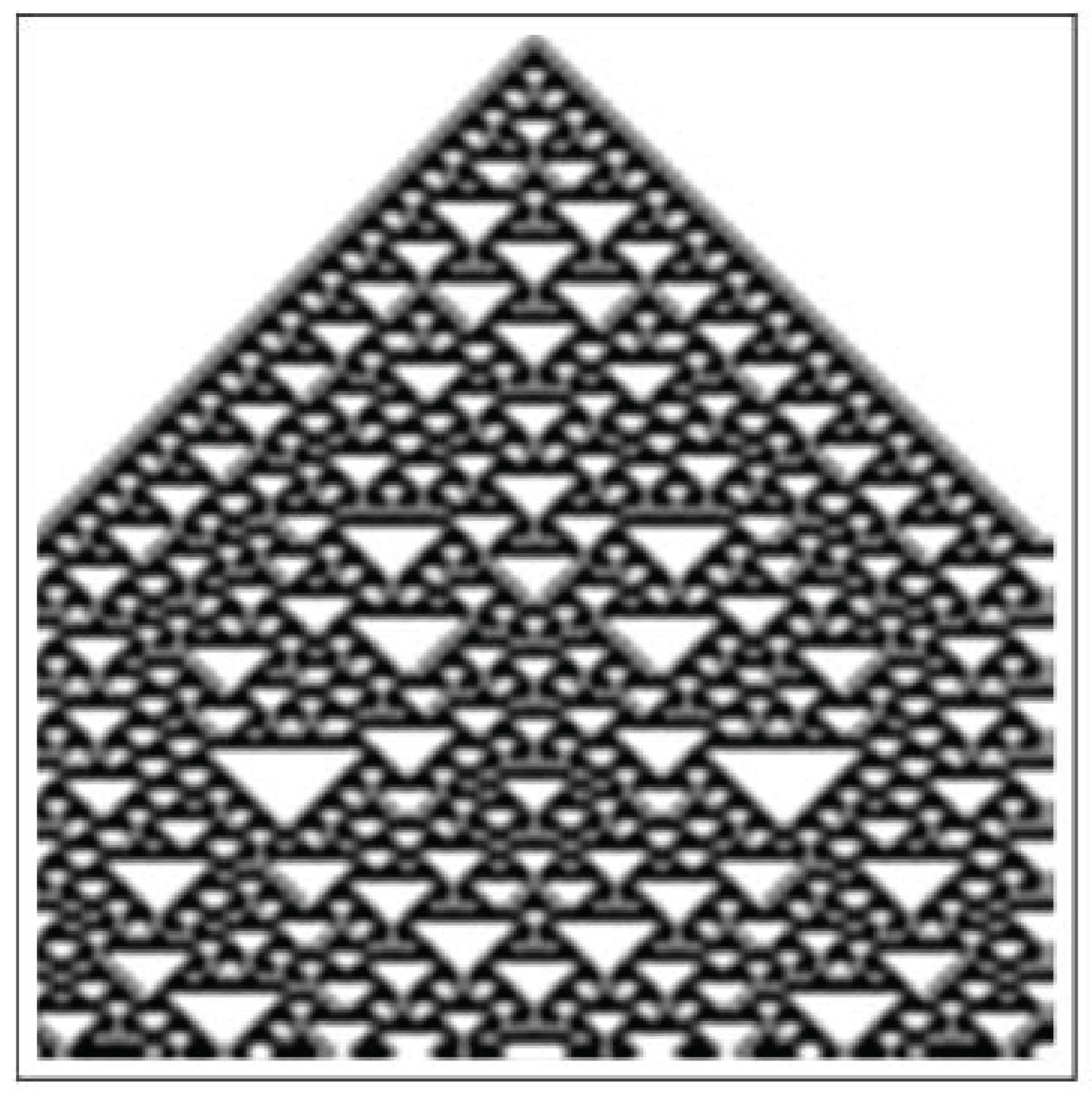
Adding some growth inhabitation—e.g., high benefits if not being obese in an otherwise obese society, say due to the huge success with the girls—can then produce complex behavior even for $k=2$; this may be a plausible description in the context of fashions with agents striving to follow the herd up to a point but to stress individualism beyond a threshold (as Yogi Berra is often quoted, "the place is so crowded, no one goes there anymore"). However to differentiate the following example from the one above, we assume in addition three states $\left(k=3\right)$ – normal $=0$, overweight $=1$, and obese $=2$—and a radius of $r=1$. This gives 27 triples but only different 7 sums under a totalistic rule, and growth inhibition is assumed for the above given reason, e.g.,

$$b_{it}=\left\{\begin{array}{c}2\\ 1\\ 0\end{array}\text{if}{B}_{i,t-1}\in \begin{array}{c}\left\{3,4\right\}\\ \left\{1,2,5\right\}\\ \left\{0,6\right\}\end{array}\right\}$$

(37)

which produces the rule $\#471=3^5+2x{3}^4+2x{3}^3+2$ and the pattern shown in Figure 5, this time started with a single seed at 1 (another representation popular in this field, which will produce a white array = no obesity for the above rule #240 since only a minimum of 4 obese can turn a slim person into an obese one) and uniformly randomly distributed over the three categories.

Figure 4. Eating behavior according to (36) - follow the majority: eat if at least 4 out of the neighborhood of 7 (radius r = 3 and totalistic) are obese. Assuming two states (0 = normal = white, 1 = obese = black) gives the cellular automaton rule #240. Simulations are for 100 agents (circular) and 100 time steps.

Figure 4. Eating behavior according to (36) - follow the majority: eat if at least 4 out of the neighborhood of 7 (radius r = 3 and totalistic) are obese. Assuming two states (0 = normal = white, 1 = obese = black) gives the cellular automaton rule #240. Simulations are for 100 agents (circular) and 100 time steps.

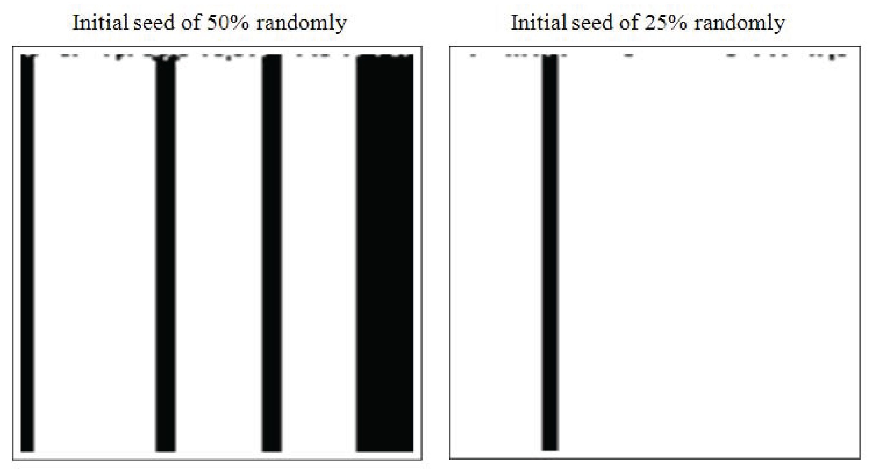
Figure 5. Eating behavior influenced by neighbors according to (37), radius r = 1, three states (k = 3): 0 = normal = white, 1 = overweight = grey, 2 = obese = black. Assuming a totalistic rule gives the cellular automaton rule #471. Simulations are for 100 agents (circular) and 100 time steps initiated by a single obese.

Figure 5. Eating behavior influenced by neighbors according to (37), radius r = 1, three states (k = 3): 0 = normal = white, 1 = overweight = grey, 2 = obese = black. Assuming a totalistic rule gives the cellular automaton rule #471. Simulations are for 100 agents (circular) and 100 time steps initiated by a single obese.

5. Final Remarks

The purpose of this paper is to highlight different mechanisms to trigger history dependent outcomes and related thresholds and to link them to social interactions. The applicability of these frameworks and of the derived conditions is demonstrated for a few examples that try to describe the phenomenon that a society may turn obese once a threshold is crossed, or finds itself across the threshold after a shock (e.g., due to unexpected low food prices). The analysis was however confined to competitive settings such that the strategic leverage of each player is negligible. Therefore a natural extension is to consider dynamic and socially related interactions where each player can influence the social reference level or norm and thus has also an interest to influence it strategically. This amounts to dynamic games which may turn out to be solvable for the first set up but hard in the case of a dynamic norm, at least for sub-game perfect Markov strategies.

References

- Wirl, F.; Feichtinger, G. History Dependence in Concave Economies. J. Econ. Behav. Organ. 2005, 57, 390–407. [Google Scholar] [CrossRef]
- Durlauf, S.N.; Young, H.P. Social Dynamics; MIT Press Cambridge: Cambridge, MA, USA, 2001. [Google Scholar]
- Burke, M.A.; Heiland, F. Social Dynamics of Obesity. Econ. Inq. 2007, 45, 571–591. [Google Scholar] [CrossRef]
- Cutler, D.M.; Glaeser, E.L.; Shapiro, J.M. Why have Americans Become more Obese? J. Econ. Perspect. 2003, 17, 93–118. [Google Scholar] [CrossRef]
- Cohen-Cole, E.; Fletcher, J.M. Is Obesity Contagious? Social Networks vs. Environmental Factors in the Obesity Epidemic. J. Health Econ. 2008, 27, 1382–1387. [Google Scholar] [CrossRef] [PubMed]
- Fowler, J.H.; Christakis, N.A. Estimating Peer Effects on Health in Social Networks: A Response to Cohen-Cole and Fletcher; Trogdon, Nonnemaker, Pais. J. Health Econ. 2008, 27, 1400–1405. [Google Scholar] [CrossRef] [PubMed]
- Miller, B.J.; Lundgren, J.D. An Experimental Study of the Role of Weight Bias in Candidate Evaluation. Obesity 2010, 18, 712–718. [Google Scholar] [CrossRef] [PubMed]
- Cooper, R.; John, A. Coordinating Coordination Failures in Keynesian Models. Quart. J. Econ. 1988, CII, 441–463. [Google Scholar] [CrossRef]
- Mailath, G.J.; Postlewaite, A. The Social Context of Economic Decisions. J. Eur. Econ. Assoc. 2003, 1, 354–362. [Google Scholar] [CrossRef]
- DeMarzo, P.M.; Vayanos, D.; Zwiebel, J. Persuasion Bias, Social Influence and Unidimensional Opinions. Quart. J. Econ. 2003, 118, 651–667. [Google Scholar] [CrossRef]
- Glaeser, E.L.; Scheinkman, J.A. Non-Market Interaction. In Advances in Economics and Econometrics: Theory and Applications. Eighth World Congress; Dewatripoint, M., Hansen, L.P., Turnovsky, S., Eds.; Cambridge University Press: Cambridge, MA, USA, 2003; Volume 1, pp. 339–369. [Google Scholar]
- Glaeser, E.L.; Sacerdote, B.I.; Scheinkman, J.A. The Social Multiplier. J. Eur. Econ. Assoc. 2003, 1, 345–353. [Google Scholar] [CrossRef]
- Wirl, F. Social Interactions within a Dynamic Competitive Economy. J. Optimiz. Theor. Appl. 2007, 133, 385–400. [Google Scholar] [CrossRef]
- Brekke, K.A.; Kverndokk, S.; Nyborg, K. An Economic Model of Moral Motivation. J. Public Econ. 2003, 87, 1967–1983. [Google Scholar] [CrossRef]
- Krugman, P. History versus Expectations. Quar. J. Econ. 1991, CVI, 651–667. [Google Scholar] [CrossRef]
- Arthur, W.B. Increasing Returns and Path Dependence in the Economy; The University of Michigan Press: Ann Arbor, MI, USA, 1994. [Google Scholar]
- Wirl, F.; Feichtinger, G. History versus Expectations: Increasing Returns or Social Influence? J. Socio-Econo. 2006, 35, 877–888. [Google Scholar] [CrossRef]
- Hof, F.X.; Wirl, F. Wealth Induced Multiple Equilibria in Small Open Economy Versions of the Ramsey Model. Homo Oeconomicus 2008, 25, 1–22. [Google Scholar]
- Barro, R.J.; Sala-i-Martin, X. Economic Growth; Mc Graw Hill: Columbus, OH, USA, 1995. [Google Scholar]
- Becker, G.S.; Murphy, K.M. A Theory of Rational Addiction. J. Polit. Econ. 1988, 96, 675–700. [Google Scholar] [CrossRef]
- Wirl, F. Stability and Limit Cycles in Competitive Equilibria Subject to Adjustment Costs and Dynamic Spillovers. J. Econ. Dynamics Control 2002, 26, 375–398. [Google Scholar] [CrossRef]
- Wirl, F. Stability and Limit Cycles in One-Dimensional Dynamic Optimizations of Competitive Agents with a Market Externality. J. Evol. Econ. 1997, 7, 73–89. [Google Scholar] [CrossRef]
- Dockner, E.; Feichtinger, G. Cyclical Consumption Patterns and Rational Addiction. Amer. Econ. Rev. 1993, 83, 256–263. [Google Scholar]
- Ryder, H.E., Jr.; Heal, G.M. Optimal Growth with Intertemporally Dependent Preferences. Rev. Econ. Stud. 1973, 40, 1–31. [Google Scholar] [CrossRef]
- Wirl, F.; Feichtinger, G. Persistent Cyclical Consumption. Variations on the Becker-Murphy Model on Addiction. Ration. Soc. 1995, 7, 149–159. [Google Scholar] [CrossRef]
- Wolfram, S. Theory and Application of Cellular Automata: Advanced Series on Complex Systems; World Scientific Publishing: Singapore, 1986. [Google Scholar]
- Wolfram, S. Cellular Automata and Complexity: Collected Papers; Addison-Wesley Publishing Company: Reading, MA, USA, 1994. [Google Scholar]
- Wolfram, S. A New Kind of Science; Wolfram Media: Champaign, IL, USA, 2002. [Google Scholar]
- Berninghaus, S.; Schwabe, U. Conventions, Local Interaction, and Automata Networks. J. Evol. Econ. 1996, 6, 297–312. [Google Scholar] [CrossRef]
- Wirl, F. Socio-Economic Typologies of Bureaucratic Corruption and Implications. J. Evol. Econ. 1998, 8, 199–220. [Google Scholar] [CrossRef]
- Arthur, W.B. Inductive Reasoning and Bounded Rationality. Amer. Econ. Rev. 1994, 84, 406–411. [Google Scholar]
- Benabou, R.; Tirole, J. Incentives and Prosocial Behavior. Amer. Econ. Rev. 2006, 96, 1652–1678. [Google Scholar] [CrossRef]
- Bahr, D.B.; Browning, R.C.; Wyatt, H.R.; Hill, J.O. Exploiting Social Networks to Mitigate the Obesity Epidemic. Obesity 2009, 17, 723–728. [Google Scholar] [CrossRef] [PubMed]
Appendix
This appendix derives the first order conditions for the individual agent’s optimal control model, establishes the dynamic system characterizing symmetric competitive equilibria, establishes a condition for steady states, and computes finally the eigenvalues of the Jacobian, which allow to characterize the stability properties—unstable (the two eigenvalues are positive or have positive real parts), saddlepoint stable (one eigenvalue is negative the other is positive), and stable (both eigenvalues are negative or have negative real parts).
Defining the current value Hamiltonian, , the Hamiltonian maximizing condition
implies
such that the the following canonical equations system for a symmetric competitive equilibrium results,
As a consequence, at an interior steady state, the following must hold,
and thus (5). The corresponding Jacobian,
has the eigenvalues
and
The term, destroys the symmetry of the Jacobian and introduces social interactions that are not accounted for in the (static) literature on social interactions and this proves crucial.
Differentiating yields
Dividing numerator and denominator by and accounting for the equality in (5) reduces this derivative to
Therefore, since .
- 1This is opposite to [13] due a negative valued stock b and positive marginal utility from consumption, πc > 0.
© 2010 by the authors; licensee MDPI, Basel, Switzerland. This article is an open access article distributed under the terms and conditions of the Creative Commons Attribution license (http://creativecommons.org/licenses/by/3.0/.)
Share and Cite
MDPI and ACS Style
Wirl, F.; Feichtinger, G. Modelling Social Dynamics (of Obesity) and Thresholds. Games 2010, 1, 395-414. https://doi.org/10.3390/g1040395
AMA Style
Wirl F, Feichtinger G. Modelling Social Dynamics (of Obesity) and Thresholds. Games. 2010; 1(4):395-414. https://doi.org/10.3390/g1040395
Chicago/Turabian StyleWirl, Franz, and Gustav Feichtinger. 2010. "Modelling Social Dynamics (of Obesity) and Thresholds" Games 1, no. 4: 395-414. https://doi.org/10.3390/g1040395