The Dynamics of Costly Signaling

Universiteit van Amsterdam, Institute for Logic, Language, and Computation, Science Park 904,1098XH Amsterdam, Netherlands
Games 2013, 4(2), 163-181; https://doi.org/10.3390/g4020163
Submission received: 11 February 2013
/
Revised: 1 April 2013
/
Accepted: 11 April 2013
/
Published: 26 April 2013
(This article belongs to the Special Issue Advances in Evolutionary Game Theory and Applications)
Abstract
:Costly signaling is a mechanism through which the honesty of signals can be secured in equilibrium, even in interactions where communicators have conflicting interests. This paper explores the dynamics of one such signaling game: Spence’s model of education. It is found that separating equilibria are unlikely to emerge under either the replicator or best response dynamics, but that partially communicative mixed equilibria are quite important dynamically. These mixtures are Lyapunov stable in the replicator dynamic and asymptotically stable in the best response dynamic. Moreover, they have large basins of attraction, in fact larger than those of either pooling or separating equilibria. This suggests that these mixtures may play significant, and underappreciated, roles in the explanation of the emergence and stability of information transfer.
1. Introduction
How can the honesty of communication between two agents be ensured when their interests do not coincide? This is one way of framing the question Spence [1] posed in his seminal paper about job market signaling. His famous answer was that a particular structure of costly signaling can guarantee honesty in equilibrium. However, a complication typical of signaling models in this tradition is that they often have an infinite number of equilibria. Such an abundance of equilibria makes equilibrium selection a daunting task. Those seeking to address this issue have often posited equilibrium refinements with the aim of identifying only a small number of plausible equilibrium outcomes.1
This paper takes a different approach to equilibrium selection in Spence’s original model of education. Instead of applying an equilibrium refinement, Spence’s game will be embedded into two common game dynamics: the replicator and best response dynamics. These dynamics arise from very different modeling assumptions. The replicator dynamic is a paradigm example of an unsophisticated process of imitation, whereas the best response dynamic is an archetype of myopic rational behavior. Nonetheless, both have been proposed as models of learning in games [4,5]. In order to study equilibrium selection and maintenance, the dynamic stability of the equilibria in Spence’s model and the sizes of the basin of attraction of each attractor will be investigated under both these dynamics.
Section 2 reviews Spence’s game and Section 3 carries out this study into the dynamics. It is found that mixed equilibria, which are largely ignored in the signaling literature, play a very important role in the emergence and stability of information transfer. It is proven that these mixtures are Lyapunov stable in the replicator dynamic and asymptotically stable in the best response dynamic. It is also shown that these mixtures have large basins of attraction; so large, in fact, that randomly chosen initial conditions are more likely to lead to a mixture than to one of the pure equilibria, which are those generally selected by standard refinements. Since both dynamics are most easily interpreted as models of large populations, these mixtures are naturally interpreted as polymorphic market states. Additionally, when multiple separating equilibria are present in the model, only the separating equilibrium in which high quality senders use the cheapest signal that is too costly for low quality types to profit by duplicating—called the Riley equilibrium—is stable under the best response dynamic. The Riley equilibrium also has the largest basin of attraction, at least when compared with other separating possibilities, under the replicator dynamic.
These results are discussed and connected to the literature in Section 5. It is suggested that this class of mixed equilibria may play a significant, and under-appreciated, role in the explanation of information transfer in competitive markets. Due to the fact that costly signaling games arise also in models of various biological [6,7] and linguistic phenomena [8,9,10,11], these results indicate that attention to mixed equilibria may be fundamental for an understanding of the evolution of communication more generally.
2. Job Market Signaling
The standard presentation of Spence’s [1] model of education takes the form of a signaling game with two players: a worker (the sender) and an employer (the receiver); see, e.g., [12], [13], or [14] for textbook accounts. The worker knows her ability level θ, but her prospective employer does not. After observing θ, the worker chooses some level of education to purchase. The worker incurs a cost obtaining this education. It is assumed that the value of the worker to the employer is θ, and that, after observing the worker’s message (choice of e), the employer pays the worker a wage w that is equal to the employer’s expectation of θ. To model this assumption the employer is frequently presumed to seek to minimize the quadratic difference between the wage and θ, hence the payoff to the employer is given as . The payoff to the employee is .
To simplify analysis, it is typically assumed that employees are one of two types; i.e., . Denote the probability of a worker being of these types and (with ). Following Spence’s original article, let , , and , so that and . These assumptions are not necessary for the equilibrium analysis of Spence’s model, but they make the dynamical analysis of the next section tractable, so for ease of exposition they are made now.
It is well known that this game has an infinite number of perfect Bayesian equilibria. Coupled with the appropriate beliefs, they come in three flavors: pooling, separating, and hybrid. In a pooling equilibrium both types of worker send the same message and the employer offers the wage upon the receipt of this message. In this sort of equilibrium the worker does not reveal any information about her type. In a separating equilibrium, type workers send message and type workers send . The employer then offers the wage 2 upon receipt of message and 1 upon receipt of message . Education level functions as a perfect indicator of worker productivity in a separating equilibrium.
Hybrid equilibria are mixtures in which one type of worker chooses one level of education with certainty and the other type randomizes between pooling and separating. In these mixed equilibria, education level carries some information, but information transfer is imperfect. An example of a particular hybrid equilibrium is given in the following section. Hybrid equilibria are often ignored in discussions of Spence’s signaling game2, but the dynamic analysis presented in the rest of this paper suggests that they may play an important role in the informational structure of markets.
So there are three types of equilibria and a continuum of each type. Many refinements have been proposed to limit this variety to just the reasonable equilibria. Indeed, the signaling and screening refinement literature is so immense that it is impossible to summarize even a small fraction of it here. Here, however, are two influential refinements. Riley [17] showed (in a more general model) that there is a unique equilibrium that Pareto dominates the family of separating equilibria, and this equilibrium (sometimes called the Riley equilibrium) is one in which high quality senders use the cheapest signal that is too costly for low quality senders to duplicate. In light of this fact, it is natural to think that if a market finds its way to a separating equilibrium, we should expect it to be the Riley equilibrium. After all, why would high quality senders invest in a more expensive signal than is necessary? In terms of Spence’s model as described above, the Riley equilibrium is the separating equilibrium with . In a different approach to equilibrium selection, Cho and Kreps [18] suggested refining beliefs off the equilibrium path. Their Intuitive Criterion, as applied to Spence’s model, has a great deal of bite. It eliminates all equilibrium outcomes except the Riley equilibrium. In a related paper Cho and Sobel [16] analyze another refinement of off equilibrium path beliefs that selects the Riley equilibrium in this game.3
Nöldeke and Samuelson [2] pioneered an alternative approach to equilibrium selection in Spence’s model. Finding inspiration in Spence’s remark that certain equilibrium outcomes would not survive a dynamic process of belief and strategy revision coupled with arbitrarily small perturbations, they investigated such a dynamic model explicitly. Their “Spencian" dynamic leads to one of three types of recurrent sets. One such set is the Riley equilibria. Another contains pooling equilibria. The third contains a two period cycle. The cycles consists of type senders always sending the message and type senders switching between sending and on each iteration of the dynamic. These cycles roughly correspond to the hybrid equilibria described above, and Nöldeke and Samuelson show that this cycle exists if an only if there is a mixed sequential equilibrium of the variant of Spence’s model developed in [18]. This approach has been further pursued by Jacobsen et al. [3], who extended Young’s [19] stochastic dynamic for agents with limited memories to games of incomplete information. They found that this stochastic process yields a strong prediction: whenever the signaling game has separating equilibria, in the long-run this system’s limiting distribution will put almost all its weigh on the Riley equilibrium.
Here a complementary approach is pursued. Instead of investigating a dynamic tailor-made for Spence’s game (like Nöldeke and Samuelson [2]) or the limiting distribution of a Markov process (like Jacobsen et al. [3]), I will simply embed this game into the two most vanilla learning dynamics around (the replicator and best response dynamics). Section 5 compares the results yielded by these different approaches.
3. Pruning Spence’s Game
The previous section reviewed how it is that message cost structure can allow honest signaling in equilibrium. However, a purely static analysis limited to a game’s equilibrium structure leaves some important questions unanswered. For example, how likely is it that a population of senders and receivers ends up at a separating equilibrium instead of at pooling or at a mixture? Another unaddressed question is whether or not such a population is guaranteed to converge to an equilibrium. Nöldeke and Samuelson’s discrete-time revision protocol did not always converge to an equilibrium, but what about more run-of-the-mill dynamical systems? Such dynamics are known to exhibit complex behavior in some circumstances. For example, neither the replicator dynamic nor the best response dynamic is guaranteed to converge to the mixed Nash equilibrium of generalized rock-paper-scissors. Instead, the population may cycle around the equilibrium or spiral outward toward the boundary of phase space under the replicator dynamic, or end up oscillating endlessly in a stable limit cycle under the best response dynamic [20]. In any case, results of this sort demonstrate the importance of understanding out-of-equilibrium play and how it can lead to—or deviate from—equilibrium.
However, in order to study the dynamics here in detail, it is necessary to prune the strategy space of Spence’s game because there is not a thoroughly developed theory of adaptive dynamics for games, and in particular asymmetric Bayesian games, with infinite strategy spaces. If the important dynamical question is understanding how a system evolves to either pooling, separating, partial communication, or non-convergence, then an obvious way to shrink the strategy space is to limit workers to just two messages: the costless message and a more expensive message . Then it is natural to focus on just three pure strategies for the worker: pool by always sending , separate by sending when type and when type , and pool by always sending . Call these strategies , , and . This restriction enables us to focus on just two pure employer strategies: act as though the signal carries no information about type by offering the pooling wage , and act as though the signal perfectly identifies the type (i.e., offer 1 if is received and offer 2 if is received). Call the former strategy and the latter . This pruned extensive form game is shown in Figure 1.4
Figure 1.
The extensive form representation of Spence’s game in which workers choose from only two levels of education and employers either act as though senders are pooling (P) or act as though the message indicates low quality (L) or act as though the message indicates high quality (H).
Figure 1.
The extensive form representation of Spence’s game in which workers choose from only two levels of education and employers either act as though senders are pooling (P) or act as though the message indicates low quality (L) or act as though the message indicates high quality (H).
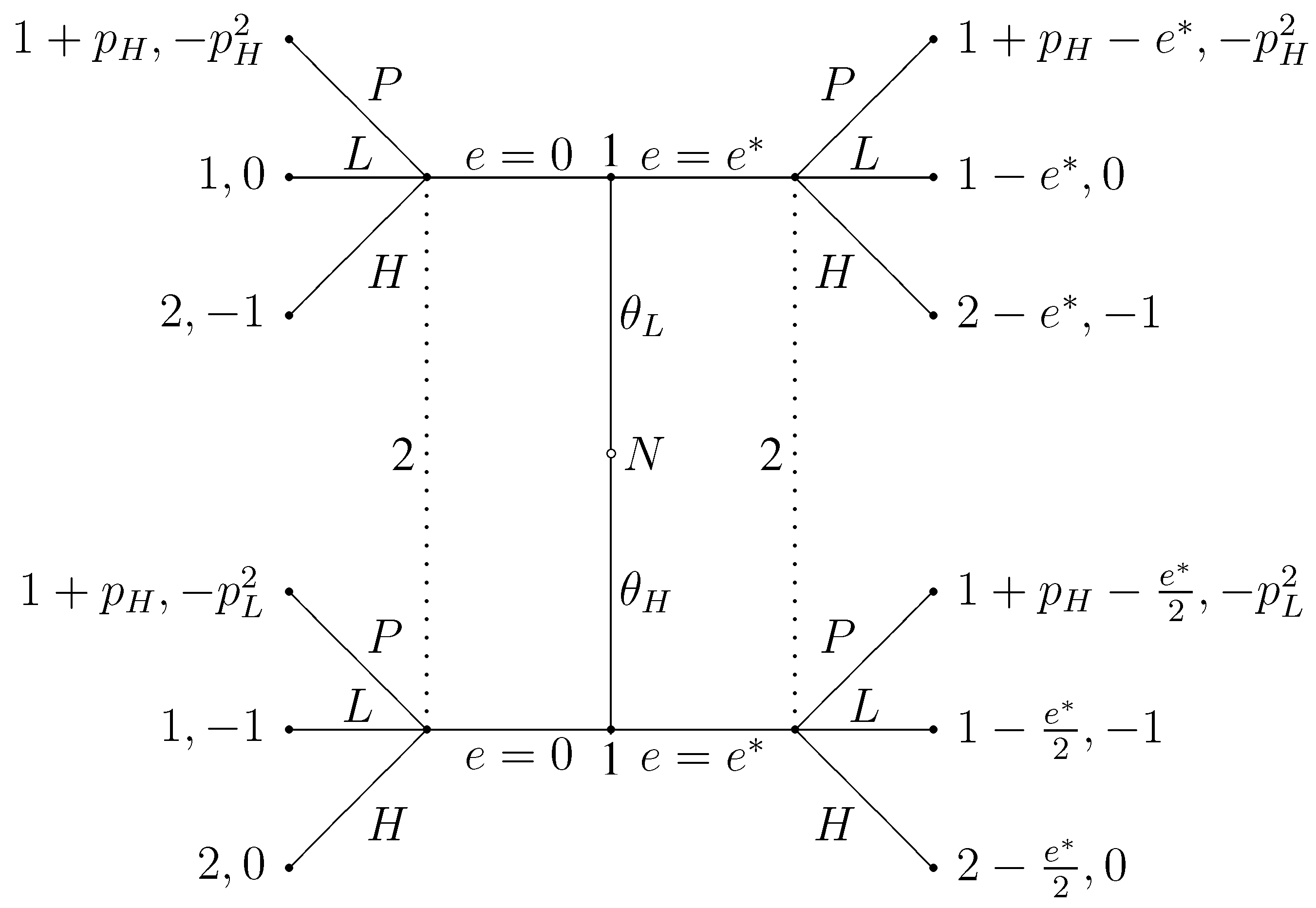
Both the replicator dynamic and the best response dynamic are infinite population models, and payoffs to strategy types are given by the type’s expected payoff when matched with a random member of the population. Therefore, we can now focus analysis on the normal game shown in Table 1 in which the payoffs are the expectations of payoffs from the extensive form game. Notice that if the receiver plays , the sender’s unique best response is to play . Likewise, the receiver’s best response to is to play . Thus, the profile is a strict Nash equilibrium. It corresponds to a pooling equilibrium in Spence’s original game; workers do not purchase education and employers do not listen to signals.
Similarly, the receiver’s unique best response to is to play . Likewise, the receiver’s unique best response to a sender who separates is to play herself. These best response relationships are independent of the cost of the more expensive message, . To determine the equilibrium structure of this game, It only remains to determine sender’s best response to a receiver playing the pure strategy . will be the sender’s unique best response if and only if . Accordingly, when , the profile corresponds to a separating equilibrium in the full game.
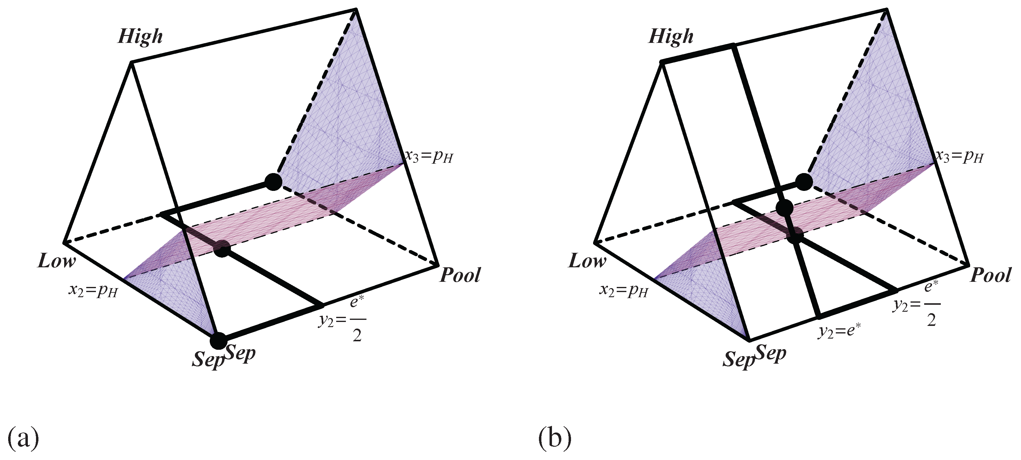
On the other hand, if then this separating profile is not an equilibrium. Nonetheless, an important mixed equilibrium exists for these values of . The profile in which the sender randomizes between and with probabilities and , and the receiver randomizes between and with probabilities and respectively is a Nash equilibrium when . It corresponds to a hybrid equilibrium in the original game in which high productivity workers send message with certainty and low productivity workers randomize between separating from and pooling with the high type. The mixed strategy space and best response correspondences for both cases are drawn in Figure 2. These correspondences are crucial for analyzing the best response dynamic below.

Figure 2.
Best response correspondences for the pruned Spence signaling game with (a) and (b) . The sender’s best reply is shown by the thick line. The receiver’s best reply is shown by the translucent surface. signifies the probability that the sender plays , the probability that the sender plays , and the probability that the receiver plays . Nash equilibria are highlighted by black dots.
Although this game has eliminated an infinite number of sending and receiving strategies, it still captures the spirit of Spence’s model. Pooling is always an equilibrium outcome, and separating can be an equilibrium if the high quality types send a sufficiently costly message. Thus, just like in Spence’s model, a costly education can signal high quality and secure high wages even though education itself may not increase productivity. Now that we have a two player normal form game that retains some of the structure of Spence’s original model, it is possible to proceed in analyzing the dynamics of job market signaling.
4. Dynamics
The adaptive dynamics considered here are the two-population replicator and best response dynamics. The first population is the population of workers. Denote the proportion that chooses each strategy , , and as , , and . The second population consists of employers. Let and be the proportions of the population that play and . Because and , the dynamics for this system live in the three dimensional space where is the dimensional simplex . Coordinates in phase space will be written .5
The replicator dynamic for the pruned game is given by the three differential equations
where A is the sender’s payoff matrix and B is the receiver’s payoff matrix. Although this dynamic was originally formulated by [21] to model natural selection in an asexually reproducing population, it also provides a model of cultural learning in economic situations. In this context, the equations give the fluctuations in strategy distributions as agents imitate successful members of their population. In other words, these equations describe large populations of employers and workers in which individual agents, when called on to revise their strategy choice, choose to imitate a more prosperous player [22].
An advantage of focusing on the replicator dynamic is that stability analysis of its rest points can provide information about the stability of these points under all two population uniformly monotone selection dynamics. This family of game dynamics is characterized by a positive linear correlation between relative growth rates and payoff differences. Since a rest point is asymptotically stable for the replicator dynamic if and only if it is asymptotically stable under every two population uniformly monotone selection dynamic ([23], Theorem 3.5.3), studying this process provides an understanding of the behavior of this larger class of selection dynamics.
The best response dynamic for the pruned game is written as
where and is defined similarly.6 The usual interpretation of this dynamic is that a small fraction of each large population revises their strategy at each time interval. Upon revision, they choose a best reply to the current state. A complication in analyzing this system is that it is not in general differentiable at rest points (Nash equilibria) because it is at these points where abruptly changes and is often many-valued. However, an analytic virtue of this dynamic is that piecewise linear solutions can be constructed from any initial condition. This is due to the fact that, at every state, the best response dynamic moves the population in a straight line toward the current best reply profile; see, e.g. [24] or [23]. This fact will be used in the constructions below.
4.1. Separating Equilibria
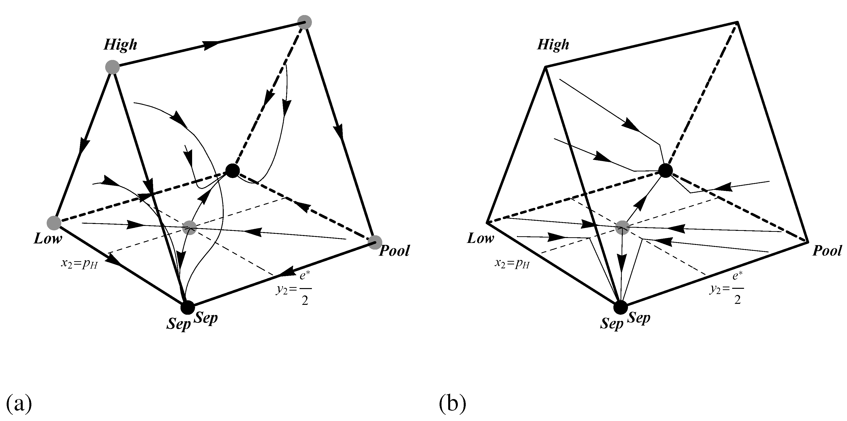
When the dynamics of the pruned game shown in Table 1 are straightforward. There are two strict Nash equilibria: and . Therefore, the corresponding states and are asymptotically stable under both dynamics. Furthermore, the pure sending strategy is strictly dominated by the pure strategy . Pure strategies that are strictly dominated by other pure strategies are driven to extinction by both dynamics. Thus every initial condition in the interior of phase space is brought to the boundary face. On this boundary face there is a mixed Nash equilibrium at . Through linearization (for the replicator dynamic) or inspection of the best response correspondences (for the best response dynamic), it is easy to see that this mixed equilibrium is unstable. Phase portraits for both systems are illustrated in Figure 3. Additionally, since asymptotically stable rest points in the replicator dynamic are asymptotically stable for every two population uniformly monotone selection dynamic, we can immediately conclude that the pooling and separating equilibria are asymptotically stable under all such dynamics.
Figure 3.
Phase portraits showing the dynamics of the pruned Spence signaling game with for (a) the replicator dynamic and (b) the best response dynamic. Black and grey dots indicate stable and unstable rest points respectively.
Figure 3.
Phase portraits showing the dynamics of the pruned Spence signaling game with for (a) the replicator dynamic and (b) the best response dynamic. Black and grey dots indicate stable and unstable rest points respectively.

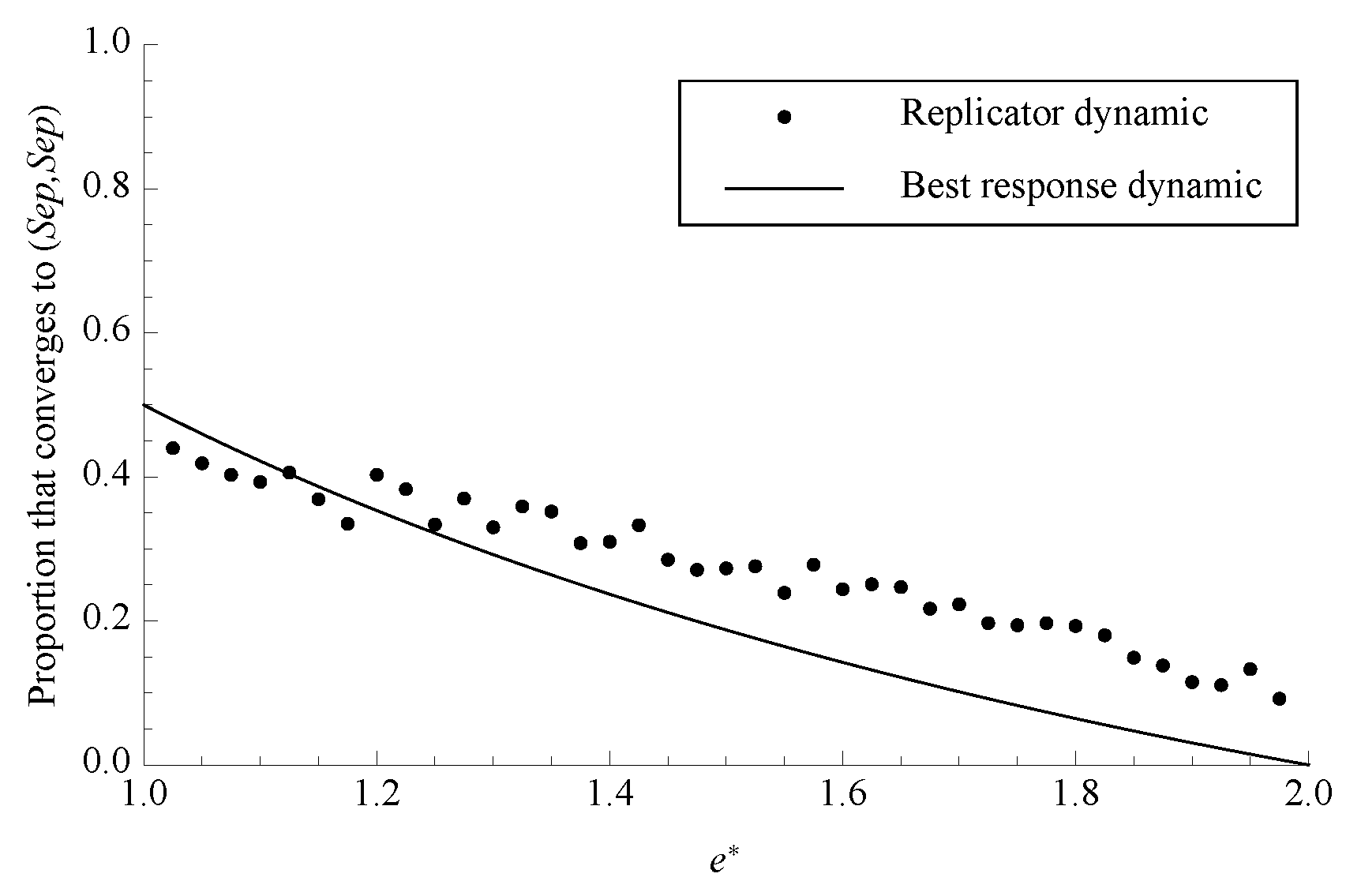
A noteworthy feature of these systems is just how small the basin of attraction for the separating equilibrium is. For the replicator dynamic, it is necessary to use numerical integration to estimate the proportion of phase space that converges to each of the strict Nash equilibria. On the other hand, for some values of that make the geometry relatively simple, the size of the basin of attraction for separating under the best response dynamic can be found analytically. The basin of attraction for separating is the portion of phase space contained within the two two-dimensional separatrices that lead directly to the unstable rest point, so for the best response dynamic it is possible to find the exact size of the basin that leads to separating by decomposing the space on the separating side of these separatrices into simple geometric figures and finding their combined volume. A chart of the proportion of phase space that leads to separating under both dynamics is shown in Figure 4.
Figure 4.
The proportion of phase space that converges to separating under both dynamics with . Each data point for the replicator dynamic is the average of 1000 randomly chosen initial conditions.
Figure 4.
The proportion of phase space that converges to separating under both dynamics with . Each data point for the replicator dynamic is the average of 1000 randomly chosen initial conditions.

4.2. Hybrid Equilibria
When , the dynamics become more complex. remains a strict Nash equilibrium and hence asymptotically stable. There are also two other rest points, each mixtures. One, at coordinates , is unstable. The other rest point lies at . This rest point corresponds to the hybrid equilibrium in which high quality workers always send and low quality workers flip a biased coin to determine whether to send or 0. Unfortunately, establishing the stability of this state is nontrivial. Linear stability analysis is inconclusive for the replicator dynamic because the rest point is not hyperbolic. Neither is linear stability analysis feasible for the best response dynamic because the dynamic is not differentiable at this location. However, the point H is indeed stable under the replicator dynamic.
Theorem 1. The hybrid equilibrium is neutrally stable under the replicator dynamic when .
Proof. See the appendix. □
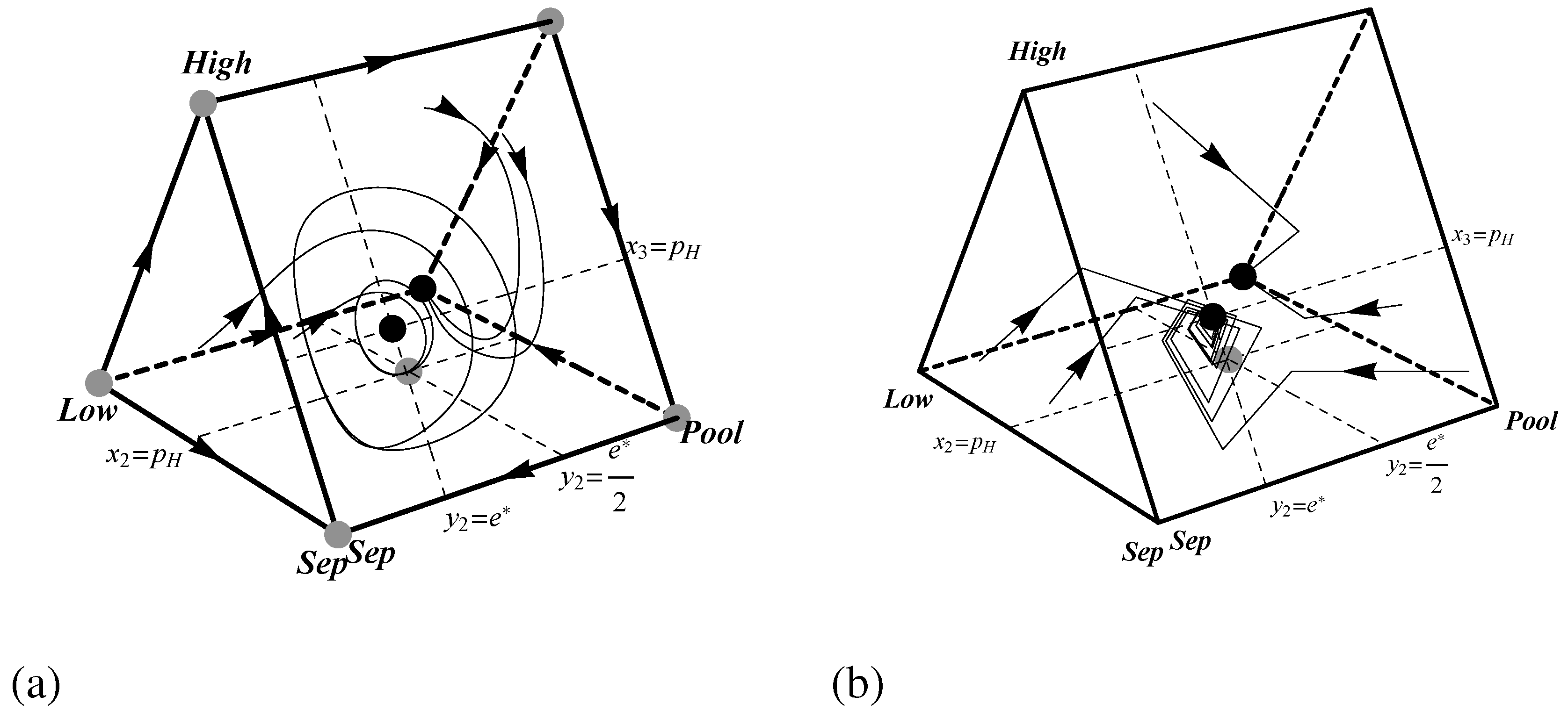
Hirsch et al. [25] call rest points like H “spiral centers." Initial conditions near H quickly spiral toward the boundary face. Then, once on this face, they cycle endlessly in closed periodic orbits centered on H. Thus, the hybrid equilibrium H is neutrally stable. Figure 5 shows a phase portrait for this system. Unfortunately, since H is not a hyperbolic rest point, nothing can be concluded about the stability of H under all uniformly monotone selection dynamics. A perturbation to the dynamic will change the system’s qualitative behavior, sending orbits, for instance, either spiraling into or away from H.
Figure 5.
Phase portraits showing the dynamics of the pruned Spence signaling game with for (a) the replicator dynamic and (b) the best response dynamic. Black and grey dots indicate stable and unstable rest points respectively.
Figure 5.
Phase portraits showing the dynamics of the pruned Spence signaling game with for (a) the replicator dynamic and (b) the best response dynamic. Black and grey dots indicate stable and unstable rest points respectively.
Although the stability of H under the best response dynamic is not as delicate, it is also not straightforward to demonstrate. Because the pruned Spence game is a non-degenerate game, the best response dynamic must approach an equilibrium [26]. This rules out the possibility that the system will enter a cycle, but does not tell us whether or not the hybrid equilibrium is stable. Nevertheless, it can be proved using a Poincaré map that H is in fact asymptotically stable under the best response dynamic.
Theorem 2. The hybrid equilibrium is asymptotically stable under the best response dynamic.
Proof. See the appendix. □
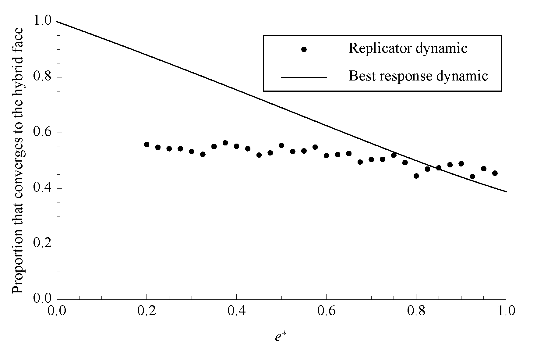
The system’s phase portraits are shown in Figure 5. Since H is not an attractor under the replicator dynamic, we cannot ask how much of phase space is attracted to H. However, since the linearization of H does have one negative eigenvalue, it is possible to investigate how much of phase space is attracted onto the boundary face. Once again, it is possible to solve for the exact proportion of phase space that is attracted to H under the best response dynamic (at least for some values of for which the geometry is not too complex). Figure 6 shows the sizes of these basins of attraction for H under both dynamics. Notice that, for all values of , a greater fraction of phase space ends in either at H or in oscillations centered on H than ended at the separating equilibrium above.
Figure 6.
The proportion of phase space that converges to the boundary face under both dynamics with . Each data point for the replicator dynamic is the average of 1000 randomly chosen initial conditions.
Figure 6.
The proportion of phase space that converges to the boundary face under both dynamics with . Each data point for the replicator dynamic is the average of 1000 randomly chosen initial conditions.
4.3. Separating vs. Hybrid Equilibria
The above showed that hybrid equilibria are stable under both dynamics and have large basins of attraction. However, so far this equilibrium type has only been pitted against pooling. Will players adopt a hybrid equilibrium even when a separating equilibrium is also an option? To approach this question, it is possible to study a slightly larger strategic form game in which pooling, separating, and hybrid equilibria all coexist. This enlarged game is shown in Table 2. In the interaction captured by this expanded game, each worker sends one of three messages: 0, , or with . The natural sending strategies include separating with high quality workers sending () and separating with those workers sending (). The corresponding receiver strategies interpret all messages less than as originating from a low quality worker () and interpret all messages less than as indicating low productivity ().
Both the replicator and best response dynamics for this game live in the five dimensional space . For , there are three stable rest points corresponding to the types of equilibria. The pooling profile and the separating profile are strict Nash equilibria and hence asymptotically stable states. There is also a hybrid equilibrium in which the sender randomizes between and and the receiver randomizes between and . This equilibrium is neutrally stable under the replicator dynamic and asymptotically stable under the best response dynamic. In fact, the replicator dynamics from Section 4.1 and Section 4.2 above are recaptured on boundary faces of the replicator dynamic for the expanded game in Table 2.
It is convenient to use the logit dynamic to estimate the proportion of the space attracted to each rest point under the best response dynamic. For small values of η, this dynamic, given here by
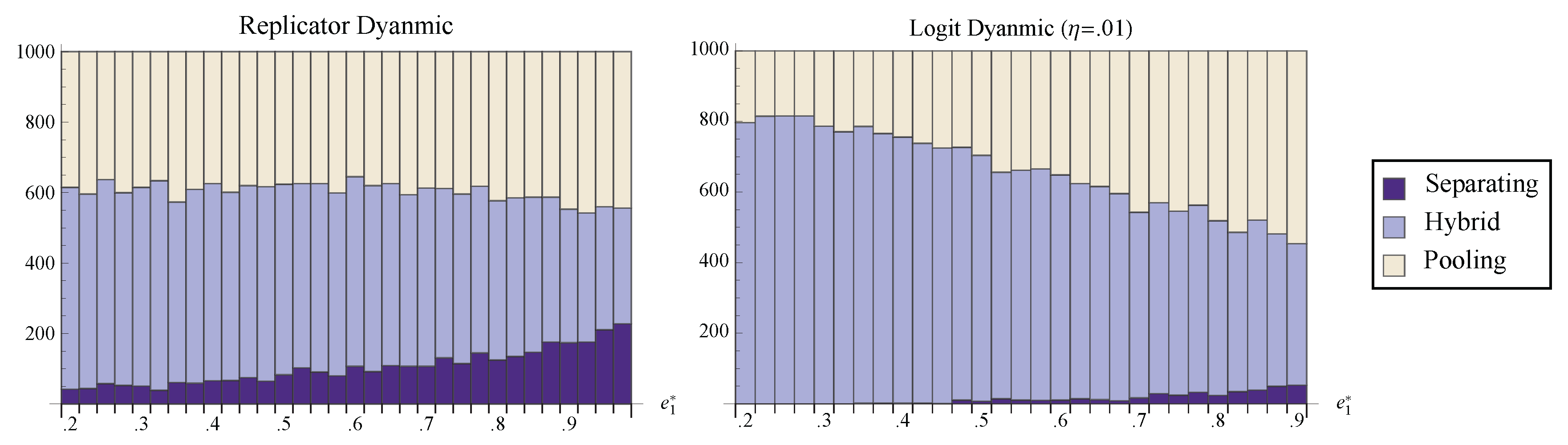
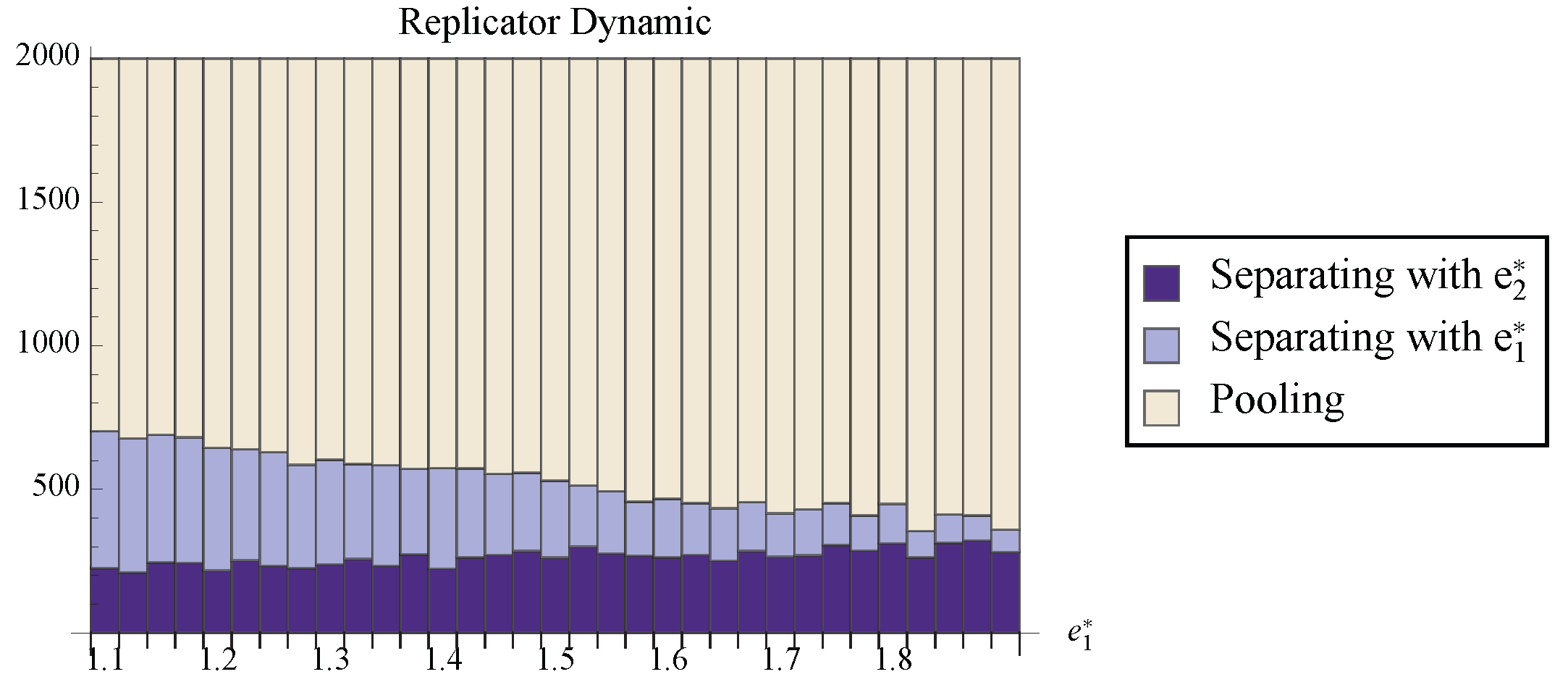
approximates the best response dynamic [27]. Figure 7 shows the number of randomly chosen initial conditions that converged to the pooling, separating, and hybrid equilibria. Notice that for all values of , the hybrid face attracts a larger portion of phase space than the separating equilibrium. Indeed, even under the best of conditions, perfect communication seems a relatively unlikely outcome of the dynamic process. Most initial states lead to partial information transfer or to no communication at all.
Figure 7.
The number of randomly chosen initial conditions that converged to pooling, separating, and the hybrid face under both the replicator dynamic and the logit dynamic with . is held fixed at while is varied.
Figure 7.
The number of randomly chosen initial conditions that converged to pooling, separating, and the hybrid face under both the replicator dynamic and the logit dynamic with . is held fixed at while is varied.
4.4. Riley Equilibria
It is also possible to use the expanded game from Table 2 to investigate which of two separating equilibria the dynamics is most likely to lead to. When , the sending strategy can be excluded to ease analysis since it is strictly dominated by . This leaves three sending strategies—, , and —with two strict Nash equilibria— and . These states are asymptotically stable under both the replicator and best response dynamics (and hence also under every two population uniformly monotone selection dynamic). There is also a Nash equilibrium component in which the sender plays and the receiver plays with probability and with probability .
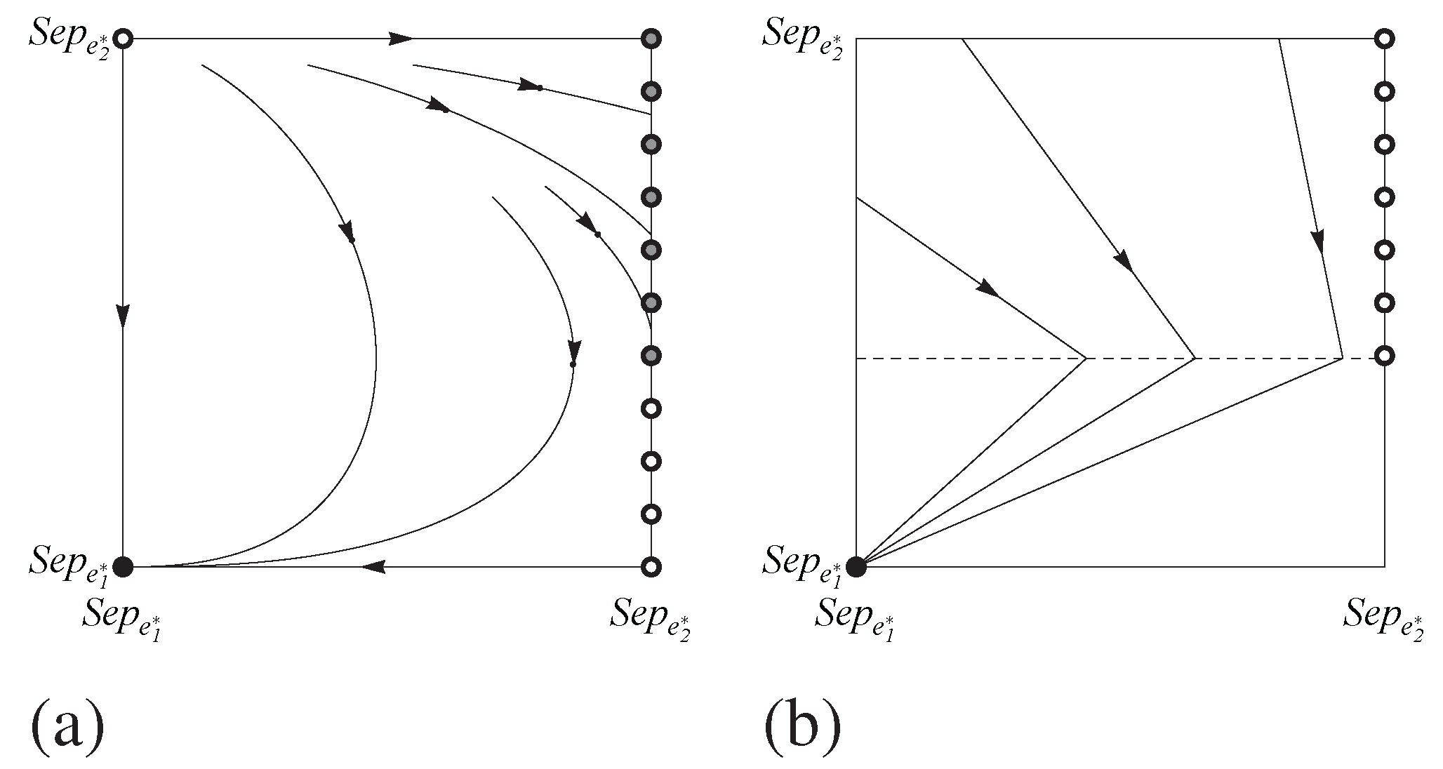
Although this Nash component constitutes a set of connected rest points under the best response dynamic, it is unstable. To see why, Figure 8 shows a phase portrait for a reduced system without the strategies and . Because the strategy profile is unstable, the best response dynamic provides a rather strong device for equilibrium selection. If the system evolves to a separating equilibrium, it will be the one in which high quality senders use the cheapest signal that is too costly for low quality senders to gain by sending. In other words, the best response dynamic here predicts that the system will arrive at what [2] call the Riley equilibrium.
Figure 8.
Phase portraits for the game in Table 2 limited to the sending and receiving strategies and for (a) the replicator dynamic and (b) the best response dynamic. The horizontal direction shows the sending population and the vertical direction shows the receiving. Black, grey, and white dots indicate asymptotically stable, neutrally stable, and unstable rest points respectively.

This Nash component is also part of a line of rest points connecting the receiver strategies and under the replicator dynamic. Here, unlike the flow for the best response dynamic, every point on the interior of this component is neutrally stable. Figure 8 provides some visual intuition, and Figure 9 shows the fraction of randomly chosen initial conditions that ended at each attracting set for the replicator dynamic. Notice that, although the stable line can have a rather large basin of attraction, it is still true that the separating state with the cheaper signal attracts a larger proportion of the space. So although the replicator dynamic does not provide as strong of prediction as the best response dynamics, the results suggest that the Riley equilibrium is the most likely separating outcome.
Figure 9.
The number of randomly chosen initial conditions that converged to each stable set under the replicator dynamic. For all trials, and .
Figure 9.
The number of randomly chosen initial conditions that converged to each stable set under the replicator dynamic. For all trials, and .
5. Discussion
The previous section showed that the usual predictions of equilibria refinements applied to Spence’s game are not validated by dynamic analysis in two respects. First, contrary to influential refinements such as the Intuitive Criterion, pooling is a likely result of both adaptive processes investigated above. As much as optimists may hope to rule out such uninspired states in which no information is conveyed, these non-communicative states may be the norm rather than the exception. Second, mixtures may be more likely than previously thought. Refinements often exclude hybrid equilibria from being considered rational solutions to Spence’s game. However, the dynamic analysis above demonstrates that mixtures are likely outcomes of learning and evolution. Although the hybrid is not asymptotically stable under the replicator dynamic, its boundary face can attract a large proportion of initial conditions. Even more strikingly, under the best response dynamic the hybrid is asymptotically stable and, for small values of , attracts almost all of phase space.
It is not implausible that a greater appreciation of hybrid equilibria may contribute to a more thorough understanding of real-life social interactions. Imagine that the job market was actually in an equilibrium in which types separated. In such a world, education would function as a perfect indicator of worker type, but this is perhaps somewhat unrealistic. In the actual world, for example, it is not always the case that only the highest quality workers invest the most in education. It seems perhaps more plausible that education level acts a noisy signal of type. High productivity workers invest in education, but some less productive workers pay the cost too and thereby masquerade as high quality. This is the picture of a market at a hybrid equilibrium, and it seems, prima facie, a more sober description of behavior actually seen in the world. Refinements have been too quick to exclude these mixed equilibria from consideration.
This moral is also relevant to game theoretic models of communication in biology. Spence’s model of job market signaling bears a remarkable resemblance to the structure of costly signaling models from biology. Zahavi [6] proposed that extravagant characteristics, such as the peacock’s tail, evolved because they honestly signal quality to prospective mates. According to this theory of sexual signaling, the peacock can be thought of as investing in the production of a gaudy tail in order to win access to peahens. Thus, the peacock’s tail plays the role of education in Spence’s model. Grafen [7] spelled out Zahavi’s proposal with a mathematical framework that is structurally similar to Spence’s game. However, Zahavi’s costly signaling hypothesis has recently been questioned. Arguments leveled against it include the charge that signaling equilibria leave all participants worse off [28] and the observation that signal cost is not necessary in equilibrium if there are costs imposed on out-of-equilibrium play [29].
This paper’s results suggest yet another criticism of the costly signaling hypothesis. Perhaps it is the case that, from a dynamic point of view, costly signaling is just a very unlikely outcome of the evolutionary process. Of course, this research does not immediately transfer to biological models, but studying the dynamics of such systems would be an interesting next step, the beginnings of which have recently been taken by Huttegger and Zollman [30], who have investigated the evolution of signaling in a related interaction known as the Sir Philip Sidney game. This is a costly signaling game developed as a model of begging behavior between mother birds and their chicks [31]. Using methods similar to those in this paper, Huttegger and Zollman have shown that the basin of attraction for the separating equilibrium in this game can be quite small, at least under the replicator dynamic. Their result echoes what has been shown above: although separating may be a Nash equilibrium, it may be a very unlikely outcome of evolutionary and learning dynamics. Thus, if we want to understand costly signals seen in nature, it might be prudent to look beyond separating equilibria to the game’s hybrid equilibria.
This conclusion can also be adapted for costly signaling models found in linguistics. Spence’s game has been co-opted to provide a first shot at a theory of politeness [8], the assumption being that polite messages are more costly to utter. However, although politeness may be a strict Nash equilibrium, the results seen here indicate that it may be an infrequent outcome of social learning. Similarly, linguists often use common-interest signaling games with costly signals to model a range of phenomena [9,10,11]. The conditions under which these games have evolutionarily stable and neutrally stable strategies are known [11], but the results seen here reveal that this static picture only provides part of the story. In addition to understanding the equilibrium structure (and even in addition to knowing which states have basins of attraction), we would like to know which are likely outcomes of the evolution or learning. The case study here shows that partially communicative mixed strategies may have large basins, and such information cannot be obtained through an analysis of equilibrium structure alone.
On the other hand, at least one prediction of more traditional game-theoretic analysis is recaptured through the dynamic approach above. Namely, this paper provides further evidence for the claim that the Riley equilibrium is the most likely separating outcome. Less efficient separating equilibria have much smaller basins under the replicator dynamic and are not even stable under the best response dynamic. These results buttress those from both Nöldeke and Samuelson [2] and Jacobsen et al. [3]. Nöldeke and Samuelson showed that under their Spencian dynamic the Riley equilibrium is the only stable separating equilibrium. Jacobsen et al. showed that in Young’s [19] stochastic dynamic, the Riley equilibrium is the only separating equilibrium with any weight in the system’s limiting distribution. Thus the observation that the Riley equilibrium is the most likely separating outcome is robust across a variety of models.
Acknowledgments
I would like to thank Brian Skyrms, Simon Huttegger, Michael McBride, Rory Smead, and Kevin Zollman for helpful comments on earlier drafts of this paper. I would also like to thank two anonymous referees for their very thoughtful comments.
References
- Spence, M. Job market signaling. Q. J. Econ. 1973, 87, 355–374. [Google Scholar] [CrossRef]
- Nöldeke, G.; Samuelson, L. A dynamic model of equilibirum selection in signaling markets. J. Econ. Theor. 1997, 73, 118–156. [Google Scholar] [CrossRef]
- Jacobsen, H.J.; Jensen, M.; Sloth, B. Evolutionary learning in signalling games. Game. Econ. Behav. 2001, 34, 34–63. [Google Scholar] [CrossRef]
- Schlag, K.H. Why imitate, and if so, how? A boundedly rational approach to multi-armed bandits. J. Econ. Theor. 1998, 78, 130–156. [Google Scholar] [CrossRef]
- Gilboa, I.; Matsui, A. Social stability and equilibrium. Econometrica 1991, 59, 859–869. [Google Scholar] [CrossRef]
- Zahavi, A. Mate selection: A selection for a handicap. J. Theor. Biol. 1975, 53, 205–214. [Google Scholar] [CrossRef]
- Grafen, A. Biological signals as handicaps. J. Theor. Biol. 1990, 144, 517–546. [Google Scholar] [CrossRef]
- Van Rooij, R. Being polite is a handicap: Towards a game theoretical analysis of polite linguistic behavior. In Proceedings of the 9th Conference on Theoretical Aspects of Rationality and Knowledge, Bloomington, IN, USA, 2003; pp. 45–58.
- Van Rooij, R. Signalling games select Horn strategies. Linguis. Philos. 2004, 27, 493–527. [Google Scholar] [CrossRef]
- Jäger, G. Evolutionary game theory and typology: A case study. Language 2007, 83, 74–109. [Google Scholar] [CrossRef]
- Jäger, G. Evolutionary stability conditions for signaling game with costly signals. J. Theor. Biol. 2008, 253, 131–141. [Google Scholar] [CrossRef] [PubMed]
- Fudenberg, D.; Tirole, J. Game Theory; MIT Press: Cambridge, UK, 1991. [Google Scholar]
- Gibbons, R. Game Theory for Applied Economists; Princeton University Press: Princeton, NJ, USA, 1992. [Google Scholar]
- Osborne, M.J.; Rubinstein, A. A Course in Game Theory; MIT Press: Cambridge, UK, 1994. [Google Scholar]
- Riley, J.G. Silver signals: Twenty-five years of screening and signaling. J. Econ. Lit. 2001, 39, 432–478. [Google Scholar] [CrossRef]
- Cho, I.; Sobel, J. Strategic stability and uniqueness in signaling games. J. Econ. Theor. 1990, 50, 381–413. [Google Scholar] [CrossRef]
- Riley, J. Informational equilibrium. Econometrica 1979, 47, 331–359. [Google Scholar] [CrossRef]
- Cho, I.; Kreps, D.M. Signaling games and stable equilibria. Q. J. Econ. 1987, 102, 179–221. [Google Scholar] [CrossRef]
- Young, P.H. The evolution of conventions. Econometrica 1993, 61, 57–84. [Google Scholar] [CrossRef]
- Gaunersdorfer, A.; Hofbauer, J. Fictitious Play, Shapley Polygons, and the Replicator Equation. Game. Econ. Behav. 1995, 11, 279–303. [Google Scholar] [CrossRef]
- Taylor, P.D.; Jonker, L. Evolutionarily stable strategies and game dynamics. Math. Biosci. 1978, 40, 145–156. [Google Scholar] [CrossRef]
- Weibull, J.W. Evolutionary Game Theory; MIT Press: Cambridge, UK, 1997. [Google Scholar]
- Cressman, R. Evolutionary Dynamics and Extensive Form Games; MIT Press: Cambridge, UK, 2003. [Google Scholar]
- Hofbauer, J.; Sigmund, K. Evolutionary Games and Population Dynamics; Cambridge University Press: Cambridge, UK, 1998. [Google Scholar]
- Hirsch, M.W.; Smale, S.; Devaney, R.L. Differential Equations, Dynamical Systems, & an Introduction to Chaos; Elsevier Academic Press: London, UK, 2004. [Google Scholar]
- Berger, U. Fictitious play in 2×n games. J. Econ. Theor. 2005, 120, 139–154. [Google Scholar] [CrossRef]
- Fudenberg, D.; Levine, D.K. The Theory of Learning in Games; MIT Press: Cambdrige, UK, 1998. [Google Scholar]
- Bergstrom, C.T.; Lachmann, M. Signalling among relatives. I. Is costly signalling too costly. Philosophical Transactions of the Royal Society, London 1997, 352, 609–617. [Google Scholar] [CrossRef]
- Lachmann, M.; Számadó, S.; Bergstrom, C.T. Cost and conflict in animal signals and human language. Proceedings of the National Academy of Science 2001, 98, 13189–13194. [Google Scholar] [CrossRef] [PubMed]
- Huttegger, S.M.; Zollman, K.J.S. Dynamic stability and basins of attraction in the Sir Philip Sidney game. Proceedings of the Royal Society B: Biological Sciences 2010, 277, 1915–1922. [Google Scholar] [CrossRef] [PubMed]
- Maynard Smith, J. Honest signalling: The Philip Sidney game. Anim. Behav. 1991, 42, 1034–1035. [Google Scholar] [CrossRef]
- Carr, J. Applications of Center Manifold Theory; Springer: New York, NY, USA, 1981. [Google Scholar]
- Guckenheimer, J.; Holmes, P. Nonlinear Oscillations, Dynamical Systems, and Bifurcations of Vector Fields; Springer: New York, NY, USA, 1983. [Google Scholar]
A. Proofs
Proof of Theorem 1. At H, the Jacobian matrix of the replicator dynamic for the pruned Spence signaling game reduces to
The characteristic equation has solutions and
These solutions are the eigenvalues of J. and, by hypothesis, . Therefore and , and consequently . Therefore, is real and negative, and both and are purely imaginary.
From the Center Manifold Theorem [32,33] it follows that there exists a stable manifold tangent to ’s eigenspace and a center manifold tangent to the eigenspace corresponding to and . According to the Center Manifold Theorem, since J has no eigenvalues with positive real part, the stability of rest point H depends solely on the dynamics upon the center manifold.
The center eigenspace here is simply the boundary face of phase space (indeed, the center manifold is identical to this boundary face). From inspecting the pruned game, it is easy to see that this face is characterized by a best response cycle. Indeed, the dynamics on this face are the dynamics of matching pennies. Under the two population replicator dynamic, it is well known that matching pennies yields closed periodic orbits centered on the mixed Nash equilibrium [22,23,24]. Thus, this is also the behavior of the system on the center manifold. Since the mixed Nash is neutrally stable in matching pennies, the hybrid equilibrium is neutrally stable in the pruned Spence signaling game. □
Proof of Theorem 2. This result will be shown by the construction of a first return map from to such that iteration of the map leads to H. Let
if and
otherwise. This adjustment when is necessary to guarantee that a point on returns to instead of converging to the pooling equilibria. Likewise let
with . These surfaces (shown in Figure 10) are the locations at which the solution trajectories to the best response dynamic abruptly change direction.
Figure 10.
The surfaces and are illustrated in (a) along with a solution orbit starting from . The iteration of the first return map and convergence to H is demonstrated in (b).
Figure 10.
The surfaces and are illustrated in (a) along with a solution orbit starting from . The iteration of the first return map and convergence to H is demonstrated in (b).
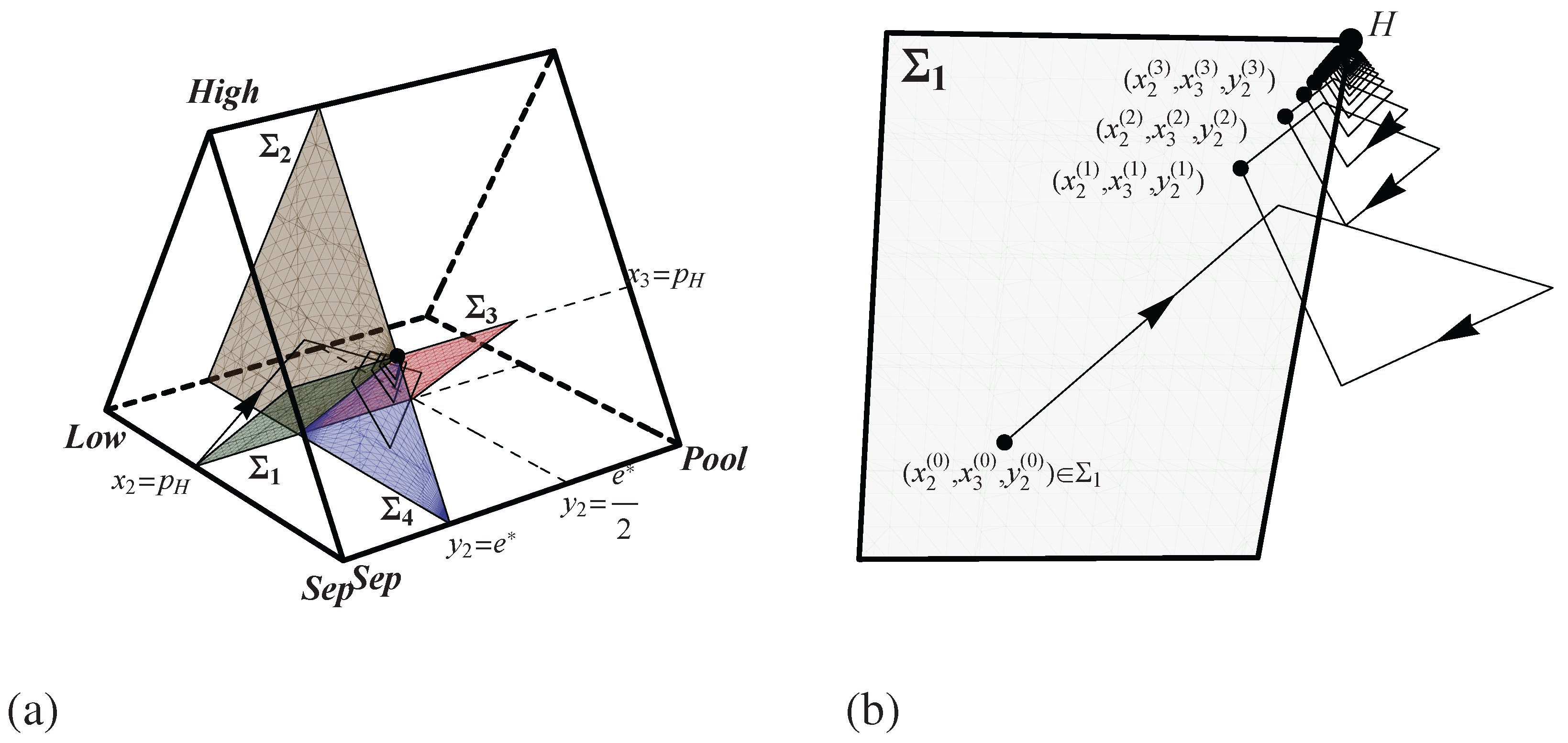
Due to the piecewise linear nature of the solution orbits, every orbit leaving each of these surfaces travels in a straight line toward the current best response profile. For instance, a solution from an initial condition on will travel in a line toward until it intersects at which point the solution changes direction to point to until intersecting , and so on. Working all this out, one can see that an initial condition on at coordinates will intersect at coordinates given by the linear equation
Then the solution will be carried to with an intersection at
Next, the solution aims to with an intersection at
Finally, the solution returns to at the location given by
Putting the four linear components together, the first return of a state on with coordinates and will be at the location given by the two dimensional map
As this fractional linear recurrence is iterated, the coordinates of the return to are
This solution (as well as all of the above linear algebra) can be easily verified in Mathematica. Looking at asymptotic behavior one sees that, and , so any initial condition on will be taken to H under the best response dynamic. Therefore, the point H is asymptotically stable. □
- 2They are not mentioned in either Fudenberg and Tirole [12] or Osborne and Rubinstein [14], and are not discussed in Spence [1]. Similarly, in his expansive survey of screening and signaling research, Riley [15] does not cover these mixtures. They are, however, discussed in Cho and Sobel [16] and Gibbons [13],
- 3.Furthermore, in the pruned Spence game that is introduced in the next section, their refinement selects the hybrid equilibrium when a separating equilibrium does not exist.
- 4Note that the interaction here is modeled as a two-player game. One player is the worker, and nature chooses her type. As was pointed out by a referee, in some economic applications it may be more natural to treat different worker types as different players. Although this is true, such a model would not be amenable to straightforward analysis in the dynamics considered here.
- 5It is convenient here to work directly with , and instead of or .
- 6Since is a set-valued function, the best response dynamic is not technically a dynamical system. Instead it is a differential inclusion.
© 2013 by the author; licensee MDPI, Basel, Switzerland. This article is an open access article distributed under the terms and conditions of the Creative Commons Attribution license (http://creativecommons.org/licenses/by/3.0/).
Share and Cite
MDPI and ACS Style
Wagner, E.O. The Dynamics of Costly Signaling. Games 2013, 4, 163-181. https://doi.org/10.3390/g4020163
AMA Style
Wagner EO. The Dynamics of Costly Signaling. Games. 2013; 4(2):163-181. https://doi.org/10.3390/g4020163
Chicago/Turabian StyleWagner, Elliott O. 2013. "The Dynamics of Costly Signaling" Games 4, no. 2: 163-181. https://doi.org/10.3390/g4020163