Article

Unraveling Results from Comparable Demand and Supply: An Experimental Investigation

1
Department of Economics, Stanford University, Stanford, CA 94305-6072, USA
2
National Bureau of Economic Research, 1050 Massachusetts Ave., Cambridge, MA 02138, USA
3
Department of Economics, Stanford University, Stanford, CA 94305-6072, USA
4
Department of Economics, Boston College, Chestnut Hill, MA 02467, USA
*
Author to whom correspondence should be addressed.
Games 2013, 4(2), 243-282; https://doi.org/10.3390/g4020243
Submission received: 30 March 2013 / Revised: 4 May 2013 / Accepted: 6 May 2013 / Published: 19 June 2013
(This article belongs to the Special Issue Games and Matching Markets)

Abstract

:
Markets sometimes unravel, with offers becoming inefficiently early. Often this is attributed to competition arising from an imbalance of demand and supply, typically excess demand for workers. However this presents a puzzle, since unraveling can only occur when firms are willing to make early offers and workers are willing to accept them. We present a model and experiment in which workers’ quality becomes known only in the late part of the market. However, in equilibrium, matching can occur (inefficiently) early only when there is comparable demand and supply: a surplus of applicants, but a shortage of high quality applicants.

1. Introduction

In many professional labor markets most entry-level hires begin work at around the same time, e.g., soon after graduating from university, or graduate or professional school. Despite a common start time, offers can be made and contracts can be signed at any time prior to the start of employment. Such markets sometimes unravel, with offers becoming earlier and more dispersed in time, not infrequently well over a year before employment will begin.1
Unraveling is sometimes a cause of market failure, particularly when contracts come to be determined before critical information is available.2 Attempts to prevent or reverse unraveling are often a source of new market design in the form of new rules or market institutions.3
It is commonly suggested, both by economists and lay participants in these markets, that unraveling results from competition related to an imbalance of demand and supply. For example, [14], writing about the market for new physicians around 1900, writes
“ The number of positions offered for interns was, from the beginning, greater than the number of graduating medical students applying for such positions, and there was considerable competition among hospitals for interns. One form in which this competition manifested itself was that hospitals attempted to set the date at which they would finalize binding agreements with interns a little earlier than their principal competitors.”
Describing the growth of early admissions to colleges, [15] quotes a 1990 U.S. News and World Report story4
“ Many colleges, experiencing a drop in freshman applications as the population of 18-year-olds declines, are heavily promoting early-acceptance plans in recruiting visits to high schools and in campus tours in hopes of corralling top students sooner.”
There is also no shortage of commentary by market participants linking excess demand for workers to unraveling.5 And indeed, a number of unraveling events seem to have been initiated by a shock to supply or demand. See e.g., [3,18] for a description of just such a development in the market for gastroenterology fellows, in which a shock that produced excess demand for fellows (i.e., a shock that led, for the first time, to fewer fellowship applicants than fellowship positions) led to unraveling that lasted for a decade.
But, when looking at a labor market, it is not uncommon for participants on both sides of the market to be nervous about their prospects, and it can be difficult to be sure which is the short side of the market. We report an experiment in which the supply and demand can be controlled in a detailed way.
The issue is that, even in a market with more applicants than positions, there may be a shortage of the most highly qualified applicants. For example, the market for law clerks has experienced serious unraveling, with positions for new graduates in some recent periods being filled two years before graduation (see [19,20,21]). [22] writes of the judges’ perception of that market as follows:
“ But why the fervent competition for a handful of young men and women when our law schools spawn hundreds of fine young lawyers every year? Very simply, many judges are not looking just for qualified clerks; they yearn for neophytes who can write like Learned Hand, hold their own in a discussion with great scholars, possess a preternatural maturity in judgment and instinct, are ferrets in research, will consistently outperform their peers in other chambers and who all the while will maintain a respectful, stoic, and cheerful demeanor.
... Thus, in any year, out of the 400 clerk applications a judge may receive, a few dozen will become the focus of the competition; these few will be aggressively courted by judges from coast to coast. Early identification of these ” precious few” is sought and received from old-time friends in the law schools - usually before the interview season even begins.”
In just the same way, there are many federal appellate court judges, but only a few dozen are considered to have highly prestigious clerkships.
A similar story can be told about college admissions. For example, [23] says
“ There are more than two thousand four-year colleges in the United States. Only about two hundred reject more students than they accept. The vast majority of American colleges accept eighty per cent or more of those who apply. But among the top fifty there is a constant Darwinian struggle to improve selectivity.”
So both law clerks and college admissions are examples of markets in which participants on each side of the market can think of themselves as being on the long side, i.e., as facing a shortage of appropriate opportunities, if they focus on an elite subset of participants on the other side of the market. In such markets it can be hard to assess the relative balance of demand and supply in field data.
We will argue that such a situation, which we call comparable demand and supply, is in fact characteristic of markets in which we should expect to see costly, inefficient unraveling. The intuition is that unraveling requires both that firms want to make early offers and that applicants want to accept them. If information about match quality evolves over time, and if one side of the market knows that it will be in short enough supply to attract a good match when the good matches become clear, then there will not be unraveling, as one side of the market will want to await the resolution of the uncertainty.6
Unraveling will cause changes in who is matched with whom, but whether this will cause big efficiency losses will depend on whether the demand and supply imbalances are such that some "mismatches" are inevitable (in which case unraveling may just cause redistribution of mismatches), or whether they can largely be avoided by awaiting information on match quality (in which case too-early matches are likely to be inefficient).
This paper reports an experiment on these issues.7 The control available in the laboratory allows us to precisely vary the conditions of demand and supply.8 Section 2 outlines the elements of a theoretical model, sufficiently to apply it to the experimental design presented in Section 3.
Although we will concentrate here on the predictions about unraveling and inefficiency as a function of demand and supply, we will also note that the theoretical framework we develop enriches the standard model of stable matching in ways that allow for some novel predictions about the effect on one side of the market of adding participants to the other side. In particular we show that, although in the standard model i.e., after uncertainty regarding the applicant quality is resolved, adding more applicants to the market is always good for firms under the Gale-Shapley [43] stable deferred-acceptance rules (cf. [44]) and the subgame perfect equilibrium prediction in our protocol, the SPE predictions of our model can reverse when we allow multiple stages of hiring with uncertainty about the applicant quality being resolved in the middle of the game.

2. The Model

Consider a market with nF firms and nA applicants. Every firm f wants to hire up to one applicant, and every applicant a can work for up to one firm. Firms and applicants have one of two possible qualities, high (h) or low (l). A matching is a mapping that (i) maps each agent to a partner on the other side of the market or leaves her unmatched, and (ii) for any firm f and applicant a, maps f to a if and only if it maps a to f. The interpretation is that a firm f and an applicant a are matched if firm f hired applicant a and applicant a works for firm f.
Unmatched firms and applicants receive a payoff of 0. If firm f and applicant a are matched with each other, they receive payoffs that depend upon their own quality, the quality of the matched partner, and a random variable. We assume every agent prefers a high quality partner to a low quality partner, and being unmatched is the least preferred alternative for each agent. For each firm f of quality i, the payoff for being matched with an applicant a of quality j is Vf(a) = uij + εa, where εa is a random variable with mean 0, and uij > 0. For each applicant a of quality i, the payoff for being matched with a firm f of quality j is Va(f) = uij + εf, where εf is a random variable with mean 0. εf and εa are identically distributed with a marginal distribution G in the interval [−a,a] where a > 0. The joint distribution of {εa} is such that there is no tie in εa that is, there are no two applicants a1 and a2 such that Games 04 00243 i019 occurs with positive probability. Similarly, the joint distribution of {εf} is such that there is no tie in εf.
A matching is ex-post stable if there is no firm-applicant pair such that, after all uncertainty is resolved, each prefers one another to her match. A matching is efficient if the sum of the payoffs of the agents is highest among all matchings after all uncertainty is resolved. A matching is qualitywise-efficient if the sum of the payoffs of agents excluding ε’s is highest among all matchings. Since ex-post there are no ties in εf and εa with probability one, firms and applicants can be strictly rank-ordered with respect to preferences. A matching is assortative if for all k ≤ min{nF,nA}, the kth best applicant is matched with the kth best firm. The market has a unique assortative matching with probability one. A matching is qualitywise-assortative if there is no firm f of quality i and applicant a of quality j such that f is matched with an applicant of lower quality than j or is unmatched, and a is matched with a firm of lower quality than i or is unmatched.9
We assume that
Games 04 00243 i001
We choose a (the bound of the ε’s) small enough such that with the above assumptions, an efficient matching is qualitywise-assortative; i.e. no agent ever prefers a low quality partner to any high quality partner. This implies that a matching is qualitywise-assortative if and only if it is qualitywise-efficient. Moreover, there is a unique ex-post stable matching (the unique assortative matching, due to the random variables ε), which is efficient.
We will be mostly interested in qualitywise efficiency or qualitywise inefficiency rather than efficiency or inefficiency, since the values of random {ε} will be rather small and this will cause small welfare losses when a qualitywise-efficient matching is not efficient.11. However, qualitywise-inefficient matchings will lead to comparatively large welfare losses.
While we denote qualities as high and low, it would be misleading to think of those as e.g., Ivy League universities and community colleges. Rather, the analogy would be between the very best colleges and some only slightly less prestigious ones. Note that in the model the firms literally hire from the same pool of applicants. Similarly, each applicant has a chance to be among the very best, or not quite make it (hence they are far from applicants who would have no chance to be accepted to a top university, no matter the final information available about them).

2.1. The Game

Firms and applicants can match in a market with early and late hiring stages. Each stage consists of several hiring periods. There are TE periods in the early hiring stage, and TL periods in the late hiring stage. The firms’ qualities, high or low, are common knowledge to all market participants at the beginning of the first period in the early hiring stage. Let Games 04 00243 i020 be the number of high quality firms in the market and Games 04 00243 i021 be the number of low quality firms.
The applicants’ qualities are uncertain and revealed only at the first period of the late hiring stage when they become common knowledge. From the beginning, it is common knowledge that a proportion Games 04 00243 i022 of applicants for some integer Games 04 00243 i023 will be of high quality, and the remaining applicants, Games 04 00243 i024 will be of low quality (for example, there might be a special distinction attached to hiring a “ top ten” applicant). To simplify the exposition, and the later experiments, we assume that all applicants have the same ex-ante probability of being of high quality, namely Games 04 00243 i022.12 The values of the random variables {ε} are realized at the beginning of the late hiring stage, and become common knowledge. The distribution of {ε} is common knowledge at the beginning of the early hiring stage.
Firms make offers to applicants, and applicants have to decide whether to accept or reject those offers right away (they cannot hold on to offers). Once an applicant has accepted an offer from a firm, the firm and the applicant are matched with each other: the applicant cannot receive any other offers and the firm cannot make any other offers.
In every period, firms that are not yet matched may decide to make up to one offer to any available applicant. A firm can make an offer again to an applicant who previously rejected its offer. Once all the firms have decided what if any offers to make, the offers become public information. Then, applicants can decide how to respond to offers they have received: whether to accept at most one offer, or reject all offers. After all applicants have decided, their actions become public information.
So the market is a multi-period game in which firms (and applicants) make simultaneous decisions with public actions, and a move by nature in the middle of the game which determines the qualities of the applicants and the {ε} perturbations of preferences over different firms and applicants.

2.2. Analysis of Unraveling

This game has many (Nash) equilibria, including ones in which every match is concluded in period 1 of the early hiring stage. For example, a strategy profile in which for each applicant a there is only one firm fa whose offer a accepts in period 1, and in which firm fa only makes an offer in period 1 to applicant a and no other offers are made or accepted, is an equilibrium. However, such equilibria will in general not be subgame-perfect. We restrict our theoretical analysis to subgame perfect equilibria (SPEs).
We partition the space of possible demand and supply relations into 3 different scenarios representing excess supply, comparable demand and supply, and excess demand for labor, respectively. The important variables will be nF, the total number of firms, Games 04 00243 i025, the number of high quality firms, nA, the total number of applicants, and Games 04 00243 i026, the total number of high quality applicants:
Case 1.
Games 04 00243 i027: Every firm can be matched with a high quality applicant, some high quality applicants remain unmatched (if Games 04 00243 i028). There is excess supply.
Case 2.
Games 04 00243 i029: Excess applicants, but shortage of high quality applicants. There is comparable demand and supply.
Case 3.
nFnA: Each applicant can be matched with a firm. There is excess demand. We analyze excess demand in two subcases:
a.
Games 04 00243 i030: Excess firms, but shortage of high quality firms.
b.
Games 04 00243 i031: Every applicant can be matched with a high quality firm, some high quality firms remain unmatched (if Games 04 00243 i032).
We will show that the SPEs of this game support the following intuition. In case 1, no firm will wish to make an early offer, because by waiting until applicants’ qualities are known, every firm can hire a high quality applicant. Thus, there is excess supply of labor.
In Case 2, in the early stage, a given applicant does not know if she will be on the long or short side of the market, since her quality is still unknown (and since there will be too few high quality applicants, and too many low quality applicants). This is why we say that there is comparable demand and supply. An applicant may therefore find it attractive to take an early offer from (even) a low quality firm, and making such an offer is profitable for a low quality firm, since this is the only way to possibly hire a high quality applicant. So Case 2 may be subject to unraveling.
Case 3a looks superficially symmetric to Case 2 but with the critical difference that the role of firms and applicants are reversed. Since the qualities of firms are already known in the early stage, no high quality firm is in any doubt that it will be on the short side of the market, and no applicant is in any doubt that she can find a position in the late period. So no applicant will take an early offer from a low quality firm (since such offers will remain available even if the applicant turns out to be low quality), and no high quality firm will make an early offer.13 Case 3b looks like Case 1 with firms and workers reversed, but in this case there is much less difference between early or late matching, since even early matchings cannot be qualitywise-inefficient, as every applicant, regardless of quality, will match to a high quality firm. Thus, we refer to Cases 3a and 3b as excess demand conditions.
We are concerned about the inefficiency (or efficiency) of SPE outcomes. We will mostly focus on “ large scale” inefficiency, namely qualitywise inefficiency. The following result characterizes the demand and supply condition in which there are qualitywise-inefficient outcomes under SPEs:
Table 1. Treatments.
nA = 6
Games 04 00243 i033
nA = 12
Games 04 00243 i034
nF = 4
Games 04 00243 i035
THIN COMPARABLE MARKET
Case 2
(baseline design)
SPE Prediction:
Low quality firms hire early qualitywise-inefficient outcome
MARKET WITH EXCESS SUPPLY
Case 1
SPE Prediction:
Late and assortative matching efficient outcome
nF = 8
Games 04 00243 i036
MARKET WITH EXCESS DEMAND
Case 3
SPE Prediction:
Late and assortative matching efficient outcome
THICK COMPARABLE MARKET
Case 2
SPE Prediction:
Low quality firms hire early qualitywise-inefficient outcome
Theorem 1 A qualitywise-inefficient early matching is an outcome of a subgame perfect equilibrium only if the market is one of comparable demand and supply (Case 2), i.e., if Games 04 00243 i029.14
Note that not all early matching equilibria are qualitywise-inefficient. For example, when Games 04 00243 i031, high firms can hire applicants early under SPE as described by Lemma 3 (in Appendix A), but the outcome will not be qualitywise-inefficient. That is the reason we concentrate on qualitywise-inefficient early hiring (as opposed to all early hiring) in Theorem 1, since only qualitywise-inefficient hiring creates large welfare problems.15 Note also that, while qualitywise-inefficient early matching cannot be a perfect equilibrium outcome except under conditions of comparable demand and supply, whether it is depends on the parameter values in a way that will be detailed in Propositions 3 and 4 in Appendix A (which is also where proofs are).

3. Experimental Design

The theoretical analysis of this simple market shows that there are a multitude of Nash equilibria. However, restricting attention to SPEs provides clear predictions. Early, qualitywise-inefficient matching can occur only when demand and supply are comparable in the sense that there is initial uncertainty whether a given applicant will be on the long or short side of the market.
However, behavior does not always conform to the predictions of SPE. Consequently we also test the theoretical predictions in laboratory experiments.
Apart from testing the SPE predictions, the experiments also allow us to distinguish these from alternative hypotheses about unraveling. As noted in the introduction, in many markets we have studied, the intuition of market participants is that unraveling results simply from a shortage of applicants.
The experimental markets have two hiring stages each of which consists of four periods, so that there is time to make multiple offers at each stage (the market is uncongested). The qualities of applicants and ε values are determined at the beginning of period 5, i.e., the first period of the late hiring stage.
We consider a design with four treatments in which there are four or eight firms, and six or twelve applicants (in all possible combinations). In each case, half the firms are of high quality, and a third of the applicants are eventually of high quality. It will be helpful to consider the treatment with the fewest firms and applicants as the baseline treatment, to which others will be compared.
We will refer to the baseline treatment as the thin comparable markettreatment, since it satisfies the Case 2 demand and supply condition, comparable demand and supply. We then change the market conditions by increasing the number of firms and workers. Doubling the number of low and high quality applicants yields the treatment referred to as the market with excess supply, satisfying the Case 1 demand and supply condition. Doubling the number of high and low quality firms, keeping the number of applicants at the baseline level, yields the market with excess demand (Case 3, in particular Case3a). The largest treatment is obtained by doubling both the number of high and low quality firms and applicants. When the number of firms and workers are both at their highest levels, we are again in the case of comparable demand and supply (Case 2), so we refer to this treatment as the thick comparable market (see Table 1).
In each market an agent earns points when she gets matched to a partner. We set uhh = 36 points, uhl = ulh = 26 points, and ull = 20 points for the preferences, which satisfy that uhhuhl > ulhull > 0. We choose the distribution of ε as follows: When there are two agents in a quality type (high quality applicants, high quality firms or low quality firms in various treatments), we set {ε1,ε2} = {−1.2,1.2}, and each permutation, i.e., (ε1,ε2) = (−1.2,1.2) and (ε1,ε2) = (1.2,−1.2), is chosen with equal probability. When there are four agents in a quality type (high quality applicants, low quality applicants, high quality firms or low quality firms in various treatments), we have {ε1,ε2,ε3,ε4} = {−1.2,−0.4,0.4,1.2}, and each permutation is chosen with equal probability. When there are eight agents in a quality type (such as low applicants in the market with excess supply), we set {ε1,ε2,ε3,ε4,ε5,ε6,ε7,ε8} = {−1.4,−1,−0.6,−0.2,0.2,0.6,1,1.4} and each permutation is chosen with equal probability.
At the beginning of each session, participants were randomly assigned their role as applicant and firm, which they kept throughout the session. Participants who were firms also kept their quality types as high quality or low quality throughout each session. In each session, the market game was played 20 consecutive times by generating new ID numbers for applicants in each market. Subjects received a $10 participation fee plus their total earnings in the session except in the treatment with excess supply, where we also gave an additional $5 participation fee to the subjects in the roles of applicants at the end of the session. The experimental points were converted to USD at the exchange rate $1 = 20 points.
The experimental sessions were run at the Computer Laboratory for Experimental Research (CLER) of the Harvard Business School using a subject pool consisting of college students (primarily from Harvard, Boston, Tufts, and Northeastern Universities) and at the Pittsburgh Experimental Economics Laboratory (PEEL) of the University of Pittsburgh using a subject pool consisting of college students (primarily from Pittsburgh, Carnegie Mellon, and Duquesne Universities). Each participant could only participate in one session. The experiment was conducted using z-Tree ([1]). We ran four sessions of the treatments requiring the most subjects, namely the excess supply treatment and the thick comparable market treatment. For the other treatments we collected seven sessions. The instructions for the excess supply market treatment are given in Appendix C. Instructions for the other treatments are similar.
Through the experiment the subject received feedback consistent with the modeling of the sequential game. That is, after each offer is made or rejected these offers and rejections were displayed on the screen of the subjects in the next period and on within the same market game. Moreover, who was available and who was not available were also public information on the screen of the subjects throughout the periods of the game. They were acknowledged of their earning in that market in experimental points. To prevent linkage as much as possible between market games, they were not reminded of their earnings of the earlier games between games.
The theoretical properties of the general model apply to the experimental design. Hence, the thin and thick comparable market treatments each fall under Case 2, the treatment with excess supply falls under Case 1, and the treatment with excess demand falls under Case 3a of the demand-supply conditions described in the previous section. It is trivial to check that our comparable market treatments satisfy the conditions of Proposition 4 in the Appendix. Therefore, the SPE predictions for each treatment are given in Table 1 via Theorem 1 and Proposition 4. The SPE predictions are thus that, we should see qualitywise in the baseline - thin comparable market treatment. As we add either only applicants or only firms (the treatments with excess supply and excess demand) efficiency should be restored. Restoring the relative balance (in the thick comparable market treatment), that is adding both firms and applicants, is predicted to bring back qualitywise-inefficient early matching.
Note that this design allows us to distinguish the SPE predictions from the alternative hypothesis that excess demand for workers (i.e., a shortage of workers) causes unraveling, since in that case there should be the most unraveling in the excess demand treatment. The excess supply treatment could well be similar according to this hypothesis, despite the asymmetric roles of firms and workers and how their qualities are revealed. The design also allows us to distinguish the SPE predictions from the congestion hypothesis that increasing the number of firms or of applicants will by itself facilitate unraveling, since the equilibrium predictions are that, moving from cell to cell in the experiment, an increase in the size of one side of the market will in some cases increase and in other cases decrease unraveling. The hypothesis can be summarized as while keeping the number of periods constant, increasing the number of applicants and firms may lead to more congestion even though subgame perfect equilibrium predictions say otherwise.

4. Experimental Results

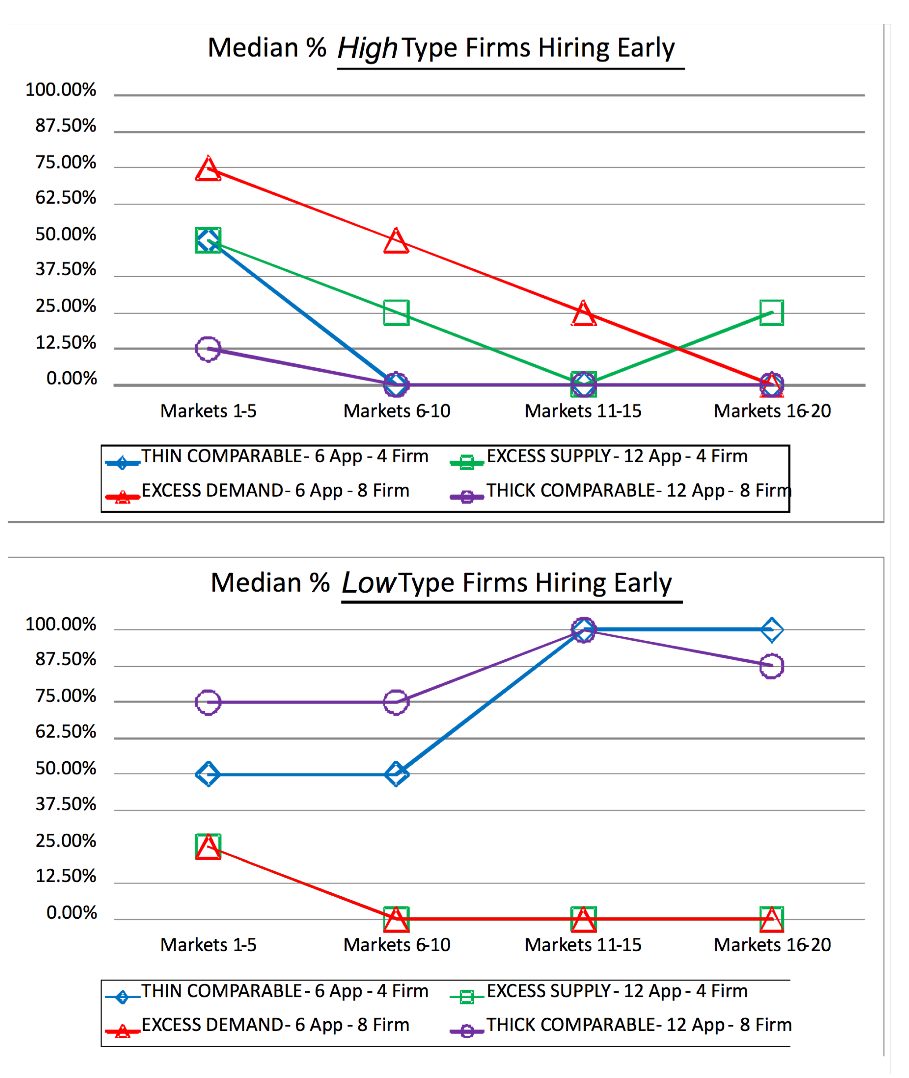
4.1. The Analysis of Matches and Unraveling

We first analyze when firms and workers match, and whether the market experiences unraveling. In every market, in all cohorts, the maximal number of matches were formed, that is, it was never the case that both a firm and a worker were unmatched. Hence, we can focus the analysis in this section on how many matches were formed in the early hiring stage, the amount of unraveling.
Figure 1 shows over time the number of firms that hire in the early stage, as they gain experience. In Table 2, we report the median of the median percentage of firms that hire early in the last five markets for each treatment.16,17 Especially in the final five markets, the observed behavior in the experiments are similar to the SPE predictions for risk-neutral subjects outlined in , although we do not observe that hiring behavior is fully consistent with SPE.
Figure 1. Median percentage of high and low type firms hiring early across treatments.
Games 04 00243 g001
Figure 1 shows that the hiring behavior moves in the direction of the SPE predictions, suggesting that there is learning over time. In the two comparable demand and supply treatments, more and more low quality firms hire early, while more and more high quality firms hire late, approaching the SPE predictions in the last five markets.
Table 2. Median percentage of firms hiring early in the last five markets, with subgame perfect equilibrium predictions in parentheses.
Actual (SPE) % Firms Hiring Early
In the last five markets - Medians
THIN COMPARABLEEXCESS SUPPLY
Low Firms 100% (100% ) 25% (0% )
High Firms 0% (0% ) 0% (0% )
EXCESS DEMANDTHICK COMPARABLE
Low Firms 0% (0% ) 87.5% (100% )
High Firms 0% (0% ) 0% (0% )
We increase excess demand when moving from the thin comparable to the excess demand treatment. The amount of early hiring in the excess demand condition refutes the hypothesis that excess demand, i.e., a shortage of applicants generates unraveling. Furthermore, unraveling in these markets is not driven primarily by congestion, since neither the excess demand or excess supply conditions experience as much early hiring as the thin comparable condition, despite having more participants.
In the excess demand condition, both high and low quality firms approach the SPE prediction of no early hiring. Using the non-parametric two-sample and two-sided Wilcoxon rank sum test, we test whether the median early hiring levels of the excess demand and the two comparable treatments are the same (in the last five markets), taking each session median for the last five markets as an independent observation. The p-values reported in Table 3 confirm that there is significantly more early hiring by low quality firms in the comparable compared to the excess demand treatments.
Similarly, the excess supply treatment also approaches SPE predictions of late hiring by both high and low quality firms (see Figure 1 and Table 3).
Table 3. Testing equivalence of high firm and low firm early hiring percentages in the last five markets. We denote significance regarding the rejection of the null hypotheses at 95% level with * and significance at 99% level with ** after the reported p-values.
H0 (For median % high/low firms hiring early)sample sizesp-value: Highp-value: Low
Thin Comparable = Thick Comparable 7,4 1 0.79
Excess Supply = Excess Demand 4,7 0.67 0.76
Thin Comparable = Excess Supply 7,4 0.56 <0.01**
Thin Comparable = Excess Demand 7,7 0.44 <0.01**
Thick Comparable = Excess Supply 4,4 0.43 0.03*
Thick Comparable = Excess Demand 4,7 0.42 <0.01**
As predicted by SPE, we cannot reject the null hypothesis that median early hiring by high quality firms in the last five markets is the same across all treatments under pairwise comparison. On the other hand, the comparable treatments have significantly higher proportions of low quality firms hiring early than the excess demand and excess supply treatments. The comparable treatments do not significantly differ from each other. Neither do the excess demand and supply treatments differ from each other.
Figure 2. Median early offer rates and acceptance rates across treatments.
Games 04 00243 g002

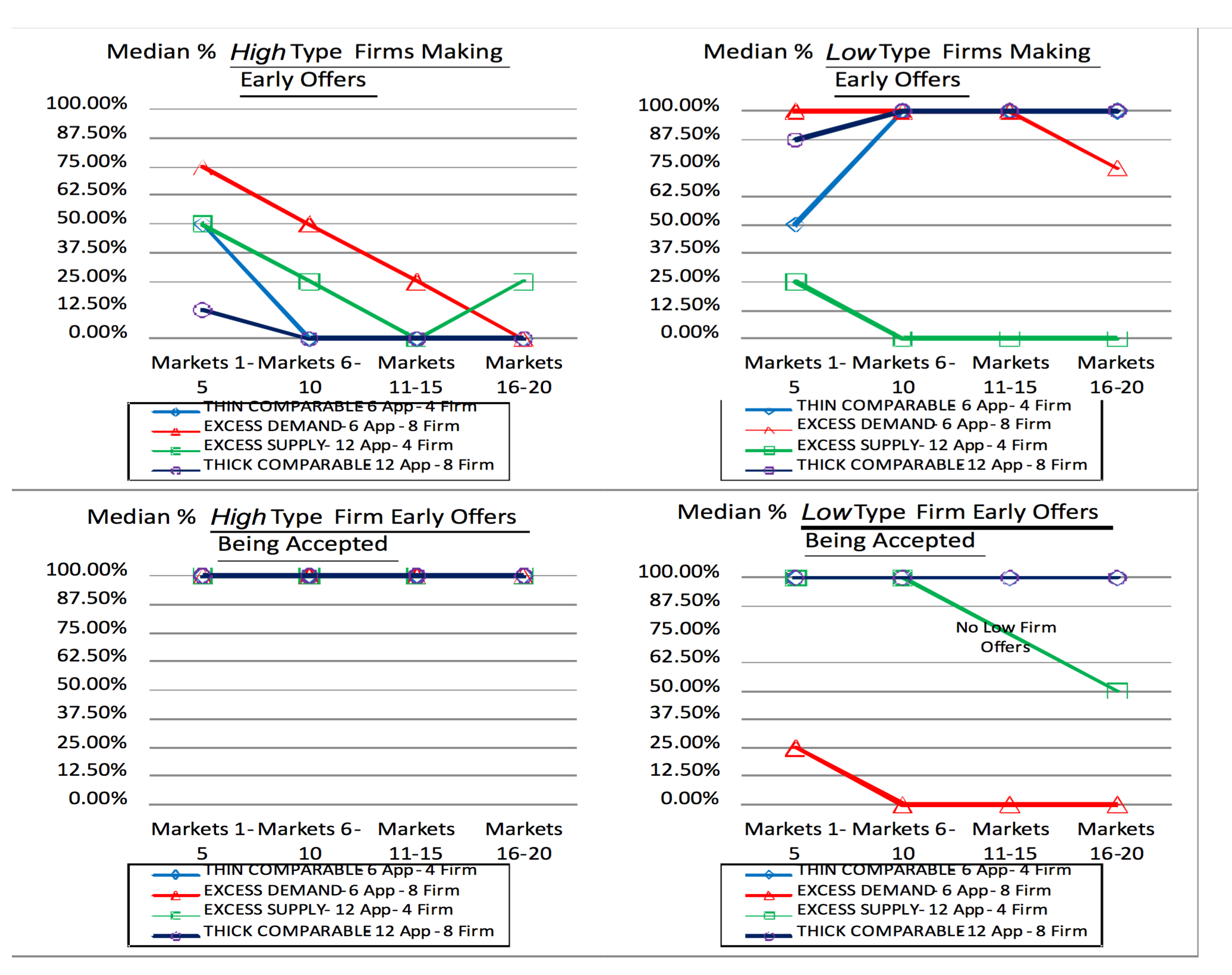
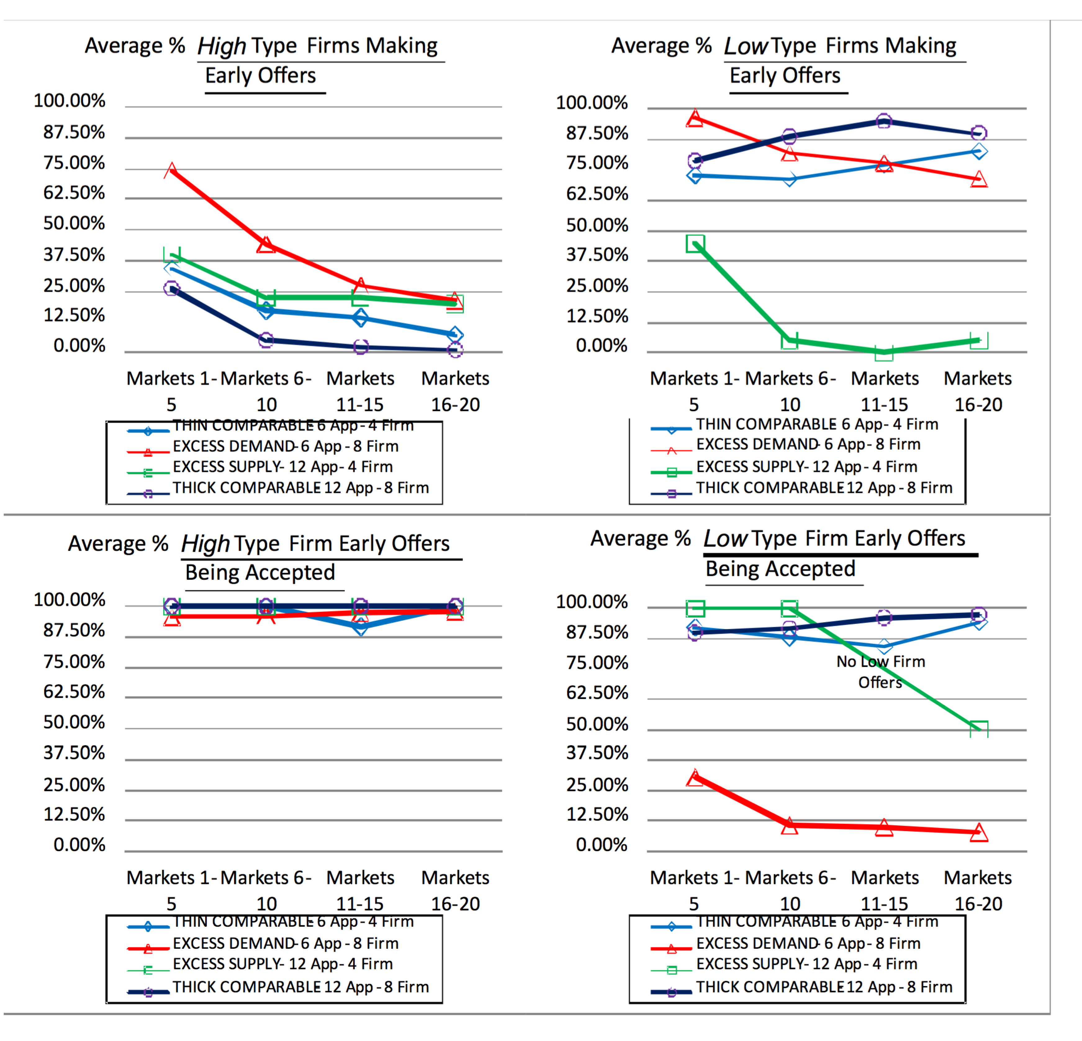
4.2. The Analysis of Early Offer and Acceptance Rates

In what follows, we examine not only the outcomes, but also the observed offer making and acceptance behavior. The top two graphs of Figure 2 show the percentage of high and low quality firms making offers in the early stage across treatments. As before, we represent markets in groups of five and report the medians of the median rates across these five market groups for each treatment. The first median mentioned is obtained across cohorts of data for each treatment. If a firm makes one or more offers in the early stage, it is counted as a firm that is making an early offer. The bottom two graphs of Figure 2 show the acceptance rates by applicants of the early offers. That is, we determine for each early offer whether it was accepted or rejected.We use the same reporting convention as before with one important difference. When there are no early offers by any firm in a market, the acceptance rate is not defined. In our median calculations, we only consider markets in which offers were actually made. This technique results in well-defined acceptance rates, even though the median offer rate is 0% in many instances. (The only exception is markets 11-15 in the excess supply treatment: no low type firms make any offers in any of these markets in any of the cohorts of data, hence we omit that acceptance rate, see the bottom right graph of Figure 2.)
We observe that the number of early offers from high type firms is decreasing and mostly converging to zero in all treatments, and that acceptance rates of high firm offers are 100%. Both of these findings are consistent with the SPE predictions both on and off the equilibrium paths. In the comparable demand and supply treatments, these percentages converge to 0% very fast. However, in the excess supply and excess demand treatments, convergence takes more time, and in the excess supply treatment we do not observe full convergence.
For early offers from low type firms and the applicants’ acceptance behavior we observe different behavior across different treatments. On and off the SPE path, predictions are such that in the comparable demand and supply treatments all low quality firms make early offers and all applicants always accept them, whenever such offers are made. Behavior in the experiment is consistent with the SPE predictions.
In the excess demand treatment, applicants should not accept early offers from low quality firms on the SPE paths. Thus, low quality firms are indifferent between making early offers and not making them at all. However, when applicants make mistakes and accept such offers, we expect low quality firms to make early offers (i.e., on a trembling hand-perfect equilibrium path). Indeed in markets 1-5, 25% of applicants accept an early offer from a low quality firm. This reinforcement seems to cause 100% of low quality firms to make early offers throughout the early markets. However, towards the final markets, early offers from low quality firms are never accepted anymore. This seems to reduce the amount of early offers from low quality firms, only 75% of them make early offers.
In the excess supply treatment, we expect low quality firms not to make early offers under SPE. Yet, off the SPE paths, when they make early offers, we expect the applicants to accept these offers. Initially, this is exactly what happens. Low quality firms almost never make early offers. However, when they make mistakes and make early offers (which is a more frequent mistake in markets 1-10, never happens in market 11-15, and only rarely in markets 16-20), applicants tend to accept those offers (as seen in the bottom right graph of Figure 2). Only in the final markets, markets 16-20, when early offers are very rare, are they accepted only 50% of the time (though this is a very small number phenomenon).18
In summary, in all treatments the behavior of the firms and applicants are mostly consistent not only with SPE predictions, but also with trembling-hand perfection predictions.

4.3. The Analysis of Efficiency

We conclude our analysis of the experimental results with qualitywise efficiency (i.e., ignoring ε’s). A full matching is an assignment under which the maximum number of firms and applicants are matched. Since for both firms and workers, matching to a high quality partner is worth more than to a low quality partner, we use the welfare of firms to provide a measure of total welfare.19 We aim to measure the proportion of gains achieved compared to the payoffs achieved by a random match that matches as many agents as possible, that is the payoffs achieved by a randomly generated full matching, where each possible full matching is equally likely. We call the sum of these expected firm payoffs the random match payoffs. Normalized (qualitywise) efficiency is defined as the sum of firm payoffs (disregarding ε values) minus the random match payoffs divided by the maximum sum of possible expected firm payoffs minus the random match payoffs (see Table 4). A value of 100% indicates that the matching in the lab achieved all possible gains compared to the average random full matching and is hence the matching that maximizes firm payoffs.20 The random match payoffs and maximum sums of possible expected firm payoffs of a full matching in each treatment are given in Table 4 along with the median of the sum of actual firm payoffs (disregarding ε values) and the normalized efficiency of the last five markets. We also report in the same table the predictions of SPE outcomes in terms of efficiency.
Table 4. Median of the sum of firm payoffs in the last five markets, with random match payoffs and maximum firm payoffs under full matchings in parentheses, and normalized efficiency, with the theoretical SPE prediction in parentheses.
In the last five markets - Medians THIN COMPARABLEEXCESS SUPPLY
Actual Firm Welfare [Random, Max.] 108 [102.67, 112] 124 [102.67, 124]
Actual (SPE) N.Efficiency= Games 04 00243 i03757% (57%)100% (100%)
EXCESS DEMANDTHICK COMPARABLE
Actual Firm Welfare [Random, Max.] 164 [154, 164] 220 [205.34, 224]
Actual (SPE)N. Efficiency= Games 04 00243 i037100% (100%)79% (79)
First note that both comparable demand and supply treatments lack full qualitywise efficiency. The median SPE outcomes predict 57% and 79% efficiency for the thin and thick comparable treatment. The outcomes are exactly aligned with the theoretical predictions.21 This reflects the earlier results that both early offers and acceptances, and hence early matches follow SPE predictions (low quality firms hire early, while high quality firms hire late).
Table 5. Testing equality of normalized efficiency in the last five markets.
H0 (For median n. efficiency) sample sizesp-value
Thin Comparable = Thick Comparable7,40.12
Excess Supply=Excess Demand4,70.73
Thin Comparable=Excess Supply7,40.33
Thin Comparable=Excess Demand7,70.021*
Thick Comparable=Excess Supply4,40.49
Thick Comparable=Excess Demand4,70.048*
When we inspected the data, we found that there is less overall early hiring in the excess demand treatment compared to the comparable demand and supply treatments. Furthermore, there is also a significantly higher proportion of efficiency realized, compared to both the thin and thick comparable treatments (the two of which are not significantly different from one another). See Table 5 for p-values of the Wilcoxon rank sum tests of median efficiency.22
In the excess supply treatment, we found that, in the last five markets a median of 25% of high type firms hire early, while low type firms do not hire early. SPE predicts that no high quality firms hire early. In the excess supply treatment, there are four high quality applicants for four firms, including the two high quality firms. A high quality firm that hires early will, however, match with a high type applicant only one third of the time. That is two thirds of the time there will be an efficiency loss of 10 points (when the high type firm only receives 26 points from hiring a low type applicant compared to the 36 from hiring a high type applicant). Since only once in every other market does a high type firm hire early, we expect about one third of all sessions to yield median efficiency below 100%. And indeed, the median efficiencies are 100%, 100%, 100%, and 53.11% (which results from one high type firm hiring a low type worker, and all other firms hiring high type workers). Hence while the median efficiency of the excess supply treatment is 100%, there is some variance, such that the efficiency is not significantly higher in the excess supply treatment compared to the comparable demand and supply treatments (see Table 5).

4.4. Further Consequences: Effects of Changing Labor Supply

The experiment confirms the theoretical prediction that, under some circumstances, the addition of agents on one side of the market can cause unraveling, or prevent it. This gives us an opportunity to revisit a robust result in the literature of static matching models about the welfare of agents on one side of the market when the number of agents on the other side of the market increases or decreases. Using the firm-optimal stable matching as the solution concept for centralized models of matching markets, [44] showed that increasing the number of applicants in the market while keeping the firm preferences unchanged within the old applicant set cannot make any firm worse off (Proposition 2, p. 264).23 We can state a similar result on our domain, if we confine our attention to the late hiring stage.
Proposition 1 For a given set of firms that remain unmatched until the late hiring stage, if the number of available applicants increases and the number of available high quality applicants does not decrease, no available firm will be ex-ante worse off under any subgame perfect equilibrium.
However, if we consider our full two-stage matching game this conclusion no longer holds. An increase in the number of applicants can move the market conditions from Case 3a, when all equilibria yield late matching, to Case 2, and an unravelled market, and this can harm some firms (a change in the number of applicants could also simply increase the amount of unraveling within Case 2. Note that Proposition 1 implies that firms can become worse off from an increase in the number of applicants only when this leads to a decrease in the number of high quality applicants available in the late hiring stage, through unraveling).
Proposition 2 It is possible that, for a given set of firms, if the number of applicants increases and the number of high quality applicants does not decrease, a firm can be ex-ante worse off at a subgame perfect equilibrium outcome.
Note also that a decrease in the number of high quality applicants can hurt firms in two ways. First, as in static models (and as in Proposition 1) a reduction in the number of potential high quality partners hurts firms in the usual way. Second, if the decrease in the number of applicants moves the market from Case 1 to Case 2, it may also change the SPE outcome from late matching to one with some unraveling, and this may further hurt the high quality firms by decreasing the amount of assortative matching. (Something like this happened in the market for gastroenterologists in the late 1990s.24 )

5. Discussion

It has been known at least since [2] that many markets unravel, so that offers become progressively earlier as participants seek to make strategic use of the timing of transactions. It is clear that unraveling can have many causes, because markets are highly multidimensional and time is only one dimensional (and so transactions can only move in two directions in time, earlier or later). So there can be many different reasons that make it advantageous to make transactions earlier.25
Thus the study of factors that promote unraveling is a large one and a number of distinct causes have been identified in different markets or in theory, including instability of late outcomes (which gives blocking pairs an incentive to identify each other early), congestion of late markets (which makes it difficult to make transactions if they are left until too late), and the desire to mutually insure against late-resolving uncertainty. There has also been some study of market practices that may facilitate or impede the making of early offers, such as the rules and customs surrounding “ exploding” offers, which expire if not accepted immediately.
In this paper we take a somewhat different tack, and consider conditions related to supply and demand that will tend to work against unraveling, or to facilitate it. There seems to be a widespread perception, in markets that have experienced it, that unraveling is sparked by a shortage of workers.
But for inefficient unraveling to occur, firms have to be willing to make early offers and workers have to be willing to accept them. Our experiment supports the hypothesis that a shortage of workers is not itself conducive to unraveling, since workers who know that they are in short supply need not hurry to accept offers by lower quality firms. Instead, in the model and in the experiment, it is comparable supply and demand that leads to unraveling, in which attention must be paid not only to the overall demand and supply, but to the supply and demand of workers and firms of the highest quality. An important feature of our model and experiments is that when there is inefficient unraveling, this is due to low type firms, but not high types, hiring early.
In our design, all market participants, in the model and in the experiment, know which of the treatments they are in, i.e., they know the supply and demand conditions. If we introduced uncertainty about the supply and demand conditions, theoretically we can likely emulate similar predictions as our model. Though, it would be interesting to see how these would reflect in an experimental environment to the behavior of subjects.
We emphasize again that the qualities of workers and firms in our model should not be taken literally as “ low” and “ high” while mapping our predictions to real markets. Being hired in our model can refer to being hired by one of the elite firms in a real market, some better than the others, and being unmatched can refer to being hired by one of the ordinary firms in a secondary market. For example, clerkships for federal appellate judges are elite positions for law school graduates. Yet, there is unraveling in this market and it seems to start in the 9th Circuit, whose judges are a little disadvantaged compared to the East Coast circuits.
Our results seem to reflect what we see in many unraveled markets, in which competition for the elite firms and workers is fierce, but the quality of workers may not be reliably revealed until after a good deal of hiring has already been completed. This observation not only helps us understand which markets unravel, but also casts new light on the welfare effects of changes in supply and demand.

Acknowledgements

The preliminary version of this study reporting pilot experiments and the latest version were presented at the ESA Meetings in Pittsburgh and Tucson, at the Winter ES Meeting in Philadelphia, and at New York University. We thank the participants for comments. We would also like to thank the editor of the special issue and an anonymous referee for valuable comments. Of course, all possible errors are our own responsibility. We used the Z-Tree software ([1]) in our experiment. We would like to gratefully acknowledge the support of the NSF.
  • 1See [2] for many examples, including markets other than labor markets in which contracts are fulfilled at around the same time but can be finalized substantially earlier, such as the market for college admissions, or for post-season college football bowls.
  • 2See e.g., [3] on how the market for gastroenterology fellows fragmented when it unraveled, or [4] on how college football bowls lost television viewership in years when teams and bowls were matched too early.
  • 3See e.g., [5,6,7,8] on the market for gastroenterologists, [9] for the markets with exploding offers such as the law-clerk matching market, [10] on the market for new American medical graduates, [11,12,13] on markets for new British doctors, and [4] on college football bowl selections.
  • 4Titled ”A Cure for Application Fever: Schools Hook More Students with Early Acceptance Offers.” (April 23).
  • 5See for example [16] on the market for new psychiatrists, or [17] on gastroenterologists.
  • 6In any model in which offers are made over time, unraveling will occur at equilibrium only if early offers are made and accepted. The theoretical model closest in spirit to the one explored here is that of [24] in which firms and workers unravel to each insure the other against an outcome that leaves their side of the market in excess supply (in an assignment model in which agents on the long side of the market earn zero). [25] looks at a model with a continuum of agents in which unraveling is driven at equilibrium by the fact that it makes later contracting less desirable because of the difficulty of finding a match when everyone else contracts early. Unraveling as insurance is further explored in [26,27,28]. Other theoretical models have unraveling (under conditions of fixed supply and demand) determined by the competition for workers as determined by how correlated firms’ preferences ([29]), or by how well connected firms are to early information about workers’ qualities ([30]), or by the establishment of certain kinds of centralized matching mechanisms ([2,12,31]), or by strategic unraveling and uncertainty imposed by the negative externality caused by an early offer of an agent ([32]). In prior experimental studies, [13,21,33] look at unraveling as a function of what kinds of centralized market clearing mechanism are available at the time when matching may be done efficiently. [9] looks at unraveling as a function of the rules governing exploding offers in a decentralized market. [34] experimentally studies a stylized model of unraveling that can be interpreted as one in which best replies to others’ decisions about when to hire are early, but not too early, compared to the mean time at which competitors are trying to hire.
  • 7There is an evolving literature on laboratory experiments regarding different aspects of matching markets. For example, [13,18,21,33], all report experiments on harmful unraveling and how centralized mechanisms can be used successfully or unsuccessfully to stop unraveling in entry-level professional labor markets. These papers report experiments using various mechanisms including stable ones in different environments. [35,36,37,38,39] report experiments on school choice mechanisms, including some stable ones, for public schools enrollment. New York and Boston school districts adopted stable mechanisms to correct market failures due to other reasons than unraveling. Other experiments on two-sided matching markets include [8,40,41,42] that report experiments on different features of decentralized matching markets.
  • 8The usual difficulties of measuring supply and demand in the field are compounded when the supply of workers of the highest quality must be evaluated.
  • 9The assortative matching is qualitywise-assortative, although the converse doesn’t hold. Note that the ε’s define an absolute standard of efficiency, but we look at qualitywise efficiency and sorting. This is because the "’s play three roles in our treatment: 1. as a technical assumption to give us uniqueness, 2. to reflect the fact that, in future field work, we expect the data might be able to distinguish quality in the large, but not preferences among applicants with similar observables (so that quality would be observable only up to the ε’s); and 3. to make clear in our model that we are not claiming that just because a market isn’t unraveled it is efficient, rather we are only claiming that avoiding unraveling avoids a large source of inefficiency, qualitywise inefficiency.
  • 10That is, high quality firms (and applicants) have a strictly higher marginal expected payoff from increasing their partner’s quality than low quality firms (and applicants). I.e., if the production function regarding a firm and worker is the sum of the pay-offs of the firm and the worker, then it is supermodular.
  • 11For example, a qualitywise efficient matching may be inefficient when the applicant with the largest " value remains unmatched while an applicant of the same quality is matched. Qualitywise efficiency or its absence is also what can generally be assessed from evaluating field data such as that obtained by using revealed preferences over choices in marriage or dating markets for estimating preferences over observables, i.e., such estimates can determine how important a potential mate’s education is in forming preferences, but cannot observe which among identically educated potential mates will have the best personal chemistry (see e.g., [45,46,47])
  • 12For risk-neutral market participants we can equivalently assume that each applicant has a probability Games 04 00243 i022 to be of high quality. We instead choose a fixed fraction to reduce variance in the experiment that follows.
  • 13There is another asymmetry between cases 2 and 3a, namely that the firms make offers, and applicants accept or reject them. However, this will not be important to determine the SPEs. It may however be important empirically, in the experiment and in the field.
  • 14Other results and proofs of this theorem and others regarding the experimental setup are in Appendix A.
  • 15In their pioneering theoretical investigation of unraveling, [24] study an assignment market with continuous payoffs in which the supply and demand are assumed to always fall in Case 2. In the early period of their model each worker has a probability of being a productive worker in period 2 (and in period 2 all workers are either productive or unproductive, and only firms matched with a productive worker have positive output). In this context, their assumption that supply and demand fall in Case 2 is that there are more workers than firms, but a positive probability that there will be fewer productive workers than firms. They find, among other things, that inefficient unraveling is more likely “the smaller the total applicant pool relative to the number of positions.” Our framework allows us to see how this conclusion depends on supply and demand remaining in Case 2. When the total applicant pool declines sufficiently, the market enters Case 3a (when the number of workers falls below the number of firms), and inefficient unraveling is no longer predicted. Moreover, we find a characterization of supply and demand conditions necessary for sequentially rational unraveling.
  • 16For the graphs and tables, for each session, for each of the markets, we compute the median of the variable in question, in this case the number of firms that hire early. We then compute the median of each market block, for markets 1–5, 6–10, 11–15, 16–20 for each session, and then the median for each market block taking these session medians as data points, to report the final variable.For example, in Session 7 of the thin comparable market treatment, in markets 1 to 5, 100%, 0%, 50%, 0%, and 0% of the high type firms are hiring early, respectively, which results in a 0% median hiring rate. In Sessions 1 to 6, medians are similarly calculated for markets 1–5 as 0%, 50%, 50%, 0%, 50%, and 50%, respectively. The median of these six sessions and Session 7 is 50%, which is marked in the top graph of Figure 1 for markets 1–5.
  • 17In Appendix B, we report alternative analyses using means instead of medians. The figures and statistical test results are similar. In general, the mean statistics are noisier than medians due to the fact that the mean takes extreme outcomes into consideration for these samples with relatively small sizes.In the main text, we use medians instead of means for two reasons:First, our statistical test is an ordinal non-parametric median comparison test (i.e., Wilcoxon rank sum test) and not a cardinal parametric mean comparison test. We chose an ordinal test based on the small sample sizes, 7 or 4 for each treatment. Second, many of the empirical distributions are truncated. I.e., even if the efficiency measure is centered around 100%, there will be no observations above 100% while depending on the variance, we will observe lower efficiency levels. Since we use percentages to compare treatments of different size, the appropriate measure of the center of a distribution seems to be a median rather than the mean due to the inevitable skewedness of the empirical distributions.
  • 18The mean early firm offer rates in the excess supply treatment are 45.00%, 5.00% 0.00%, and 5.00% within the market groups 1–5, 6–10, 11–15, and 16–20, respectively, and the mean acceptance rates are 100.00% 100.00% and 50.00% in market groups 1–5, 6–10, and 16–20, respectively. For example, 50% acceptance rate means 2.50% of the low firms on average hired early in the last market group on average.
  • 19We could also have chosen the welfare of applicants or the sum of applicant and firm payoffs in our efficiency measure. Note that all of these measures will give the same efficiency level, since a firm and a worker who are matched receive exactly the same payoff.
  • 20In each treatment, the best full matching is the qualitywise assortative matching, that is, as many high quality firms as possible are matched with high quality applicants, and as many high quality applicants as possible are matched before matching low quality applicants.
  • 21The difference in the median of the comparable treatments is due to the small market size of the thin comparable treatment. The mean of both SPE predictions generates 71.38% efficiency. Under a typical matching (i.e., a median SPE matching), in the thick comparable treatment, one low quality firm hires a high quality applicant and the other three low quality firms hire low quality applicants through unraveling, where as in the thin comparable treatment, one low quality firm hires a high quality applicant and the other low quality firm hires a low quality applicant through unraveling.
  • 22In our analysis with the averages for the last market block reported in Appendix B, we observe an average of 20–21% of high type firms making early offers which are accepted in the excess demand treatment. SPE predicts that no high quality firms hire early. However, in the excess demand condition, there are only 2 high quality applicants for 4 high quality firms. So, even if 50% of high quality firms were to hire early, efficiency would not be affected given that the other agents follow SPE strategies. And indeed, all seven of our excess demand sessions have close to average 100% efficiency despite of relatively high average of high type firms hiring early.
  • 23The firm-optimal stable matching is a stable matching that makes every firm best off among all stable matchings. It always exists in the general Gale-Shapley [43] matching model, and in many of its generalizations (see [48]). In our model, there is a unique stable matching, which is therefore the firm-optimal stable matching.
  • 24See [49] for a survey.
  • 25There can also be strategic reasons to delay transactions; see e.g., [50,51] on late bidding in internet auctions, and the experiment of [52].
  • 26This claim is stronger than what we need for the proof of this proposition. However, we will make use of this claim in the proof of Proposition 4.

References

  1. Fischbacher, U. z-tree: Zurich toolbox for ready-made economic experiments. Exp. Econ. 2007, 10, 171–178. [Google Scholar] [CrossRef]
  2. Roth, A.E.; Xing, C. Jumping the gun: Imperfections and institutions related to the timing of market transactions. Am. Econ. Rev. 1994, 84, 992–1044. [Google Scholar]
  3. Niederle, M; Roth, A.E. Unraveling reduces mobility in a labor market: Gastroenterology with and without a centralized match. J. Polit. Econ. 2003, 111, 1342–1352. [Google Scholar]
  4. Fréchette, G.; Roth, A.E.; Ünver, M.U. Unraveling yields inefficient matchings: Evidence from post-season college football bowls. Rand J. Econ. 2007, 38, 967–982. [Google Scholar] [CrossRef]
  5. Niederle, M.; Proctor, D.D.; Roth, A.E. What will be needed for the new gi fellowship match to succeed? Gastroenterology 2006, 130, 218–224. [Google Scholar] [CrossRef]
  6. Niederle, M.; Proctor, D.D.; Roth, A.E. The gastroenterology fellowship match-The first two years. Gastroenterology 2008, 135, 344–346. [Google Scholar]
  7. Niederle, M.; Roth, A.E. The gastroenterology fellowship match: How it failed, and why it could succeed once again. Gastroenterology 2004, 127, 658–666. [Google Scholar] [CrossRef]
  8. Niederle, M.; Roth, A.E. The gastroenterology fellowship market: Should there be a match? Am. Econ. Rev., Papers and Proceedings 2005, 95, 372–375. [Google Scholar] [CrossRef]
  9. Niederle, M.; Roth, A.E. Market culture: How norms governing exploding offers affect market performance. Am. Econ. J-Microecon. 2009, 1, 199–219. [Google Scholar] [CrossRef]
  10. Roth, A.E.; Peranson, E. The redesign of the matching market for American physicians: Some engineering aspects of economic design. Am. Econ. Rev. 1999, 89, 748–780. [Google Scholar] [CrossRef]
  11. Roth, A.E. A natural experiment in the organization of entry level labor markets: Regional markets for new physicians and surgeons in the u.k. Am. Econ. Rev. 1991, 81, 415–440. [Google Scholar]
  12. Ünver, M.U. Backward unraveling over time: The evolution of strategic behavior in the entry-level british medical labor markets. J. Econ. Dyn. Control 2001, 25, 1039–1080. [Google Scholar] [CrossRef]
  13. Ünver, M.U. On the survival of some unstable two-sided matching mechanisms. Int. J. Game Theory 2005, 33, 239–254. [Google Scholar] [CrossRef]
  14. Roth, A.E. The evolution of the labor market for medical interns and residents: A case study in game theory. J. Polit. Econ. 1984, 92, 991–1016. [Google Scholar]
  15. Avery, C.; Fairbanks, A.; Zeckhauser, R. The Early Admissions Game: Joining the Elite; Harvard University Press: Cambridge, MA, USA, 2003. [Google Scholar]
  16. Santos, C.W.; Sexson, S. Supporting the child and adolescent psychiatry match. J. Am. Acad. Child. Psy. 2002, 41, 1398–1400. [Google Scholar] [CrossRef]
  17. Gorelick, F.S. Striking up the match. Gastroenterology 1999, 117, 295. [Google Scholar] [CrossRef]
  18. McKinney, C.N.; Niederle, M.; Roth, A.E. The collapse of a medical labor clearinghouse (and why such failures are rare). Am. Econ. Rev. 2005, 95, 878–889. [Google Scholar] [CrossRef]
  19. Avery, C.; Jolls, C.; Posner, R.A.; Roth, A.E. The market for federal judicial law clerks. U. Chi. L. Rev. 2001, 68, 793–902. [Google Scholar] [CrossRef]
  20. Avery, C.; Jolls, C.; Posner, R.A.; Roth, A.E. The new market for federal judicial law clerks. U. Chi. L. Rev. 2007, 74, 447–486. [Google Scholar]
  21. Haruvy, E.; Roth, A.E.; Ünver, M.U. The dynamics of law clerk matching: An experimental and computational investigation of proposals for reform of the market. J. Econ. Dyn. Control 2006, 30, 457–486. [Google Scholar]
  22. Wald, P.M. Selecting law clerks. Mich. L. Rev. 1990, 89, 152–163. [Google Scholar] [CrossRef]
  23. Menand, L. The thin envelope: Why college admissions has become unpredictable. The New Yorker 2003. [Google Scholar]
  24. Li, H.; Rosen, S. Unraveling in matching markets. Am. Econ. Rev. 1998, 88, 371–387. [Google Scholar]
  25. Damiano, E.; Li, H.; Suen, W. Unravelling of dynamic sorting. The Rev. Econ. Stud. 2005, 72, 1057–1076. [Google Scholar] [CrossRef]
  26. Li, H.; Suen, W. Risk sharing, sorting, and early contracting. J. Polit. Econ. 2000, 108, 1058–1091. [Google Scholar] [CrossRef] [Green Version]
  27. Li, H.; Suen, W. Self-fulfilling early-contracting rush. Int. Econ. Rev. 2004, 45, 301–324. [Google Scholar]
  28. Suen, W. A competitive theory of equilibrium and disequilibrium unraveling in two-sided matching. RAND J. Econ. 2000, 31, 101–120. [Google Scholar] [CrossRef]
  29. Halaburda, H. Unravelling in two-sided matching markets and similarity of agents’ preferences. Working paper. 2008. [Google Scholar]
  30. Fainmesser, I.P. Social networks and unraveling in labor markets. Working paper. 2009. [Google Scholar]
  31. TSönmez, T. Can pre-arranged matches be avoided in two-sided matching markets? J. Econ. Theory 1999, 86, 148–156. [Google Scholar] [CrossRef]
  32. Echenique, F; Pereyra, J. Strategic uncertainty and unraveling in matching markets. Working paper. 2013. [Google Scholar]
  33. Kagel, J.H.; Roth, A.E. The dynamics of reorganization in matching markets: A laboratory experiment motivated by a natural experiment. Q. J. Econ. 2000, 115, 201–235. [Google Scholar] [CrossRef]
  34. Nagel, R. Unraveling in guessing games: An experimental study. Am. Econ. Rev. 1995, 85, 1313–1326. [Google Scholar]
  35. Chen, Y.; Sönmez, T. School choice: An experimental study. J. Econ. Theory 2006, 127, 202–231. [Google Scholar] [CrossRef]
  36. Pais, J.; Pintér, A. School choice and information: An experimental study on matching mechanisms. Game. Econ. Behav. 2008, 64, 303–328. [Google Scholar]
  37. Calsamiglia, C.; Haeringer, G.; Klijn, F. Constrained school choice: An experimental study. Am. Econ. Rev. 2010, 100, 1860–1874. [Google Scholar] [CrossRef]
  38. Featherstone, C.; Niederle, M. Ex ante efficiency in school choice mechanisms: An experimental investigation. Working paper. 2008. [Google Scholar]
  39. Chen, Y.; Kesten, O. School choice: Theory and experiment. Working paper. 2009. [Google Scholar]
  40. Haruvy, E.; Ünver, M.U. Equilibrium selection and the role of information in repeated matching markets. Econ. Lett. 2007, 94, 284–289. [Google Scholar] [CrossRef]
  41. Echenique, F.; Katz, G.; Yariv, L. An experimental study of decentralized matching. Working paper. 2009. [Google Scholar]
  42. Echenique, F.; Wilson, A.; Yariv, L. Clearinghouses for two-sided matching: An experimental study. Working paper. 2009. [Google Scholar]
  43. Gale, D.; Shapley, L. College admissions and the stability of marriage. Am. Math. Mon. 1962, 69, 9–15. [Google Scholar] [CrossRef]
  44. Gale, D.; Sotomayor, M. Ms. Machiavelli and the stable matching problem. Am. Math. Mon. 1985, 92, 261–268. [Google Scholar]
  45. Banerjee, A.; Duflo, E.; Ghatak, M.; Lafortune, J. Marry for what? Caste and mate selection in modern india. working paper. MIT: Cambridge, MA, USA, 2009. [Google Scholar]
  46. Hitsch, G.J.; Hortacsu, A.; Ariely, D. Matching and sorting in online dating. Am. Econ. Rev. 2010, 100, 130–163. [Google Scholar] [CrossRef]
  47. Lee, S. Preferences and choice constraints in marital sorting: Evidence from korea. working paper. 2009. [Google Scholar]
  48. Roth, A.E.; Sotomayor, M. Two-Sided Matching: A Study in Game-Theoretic Modeling and Analysis; Cambridge University Press: Cambridge, UK, 1990. [Google Scholar]
  49. Niederle, M.; Roth, A.E. The effects of a central clearinghouse on job placement, wages, and hiring practices. Autor, D., Ed.; In Labor Market Intermediation; The University of Chicago Press: Chicago, IL, USA, 2009; pp. 199–219. [Google Scholar]
  50. Roth, A.E.; Ockenfels, A. Last-minute bidding and the rules for ending second-price auctions: Evidence from ebay and amazon auctions on the internet. Am. Econ. Rev. 2002, 92, 1093–1103. [Google Scholar] [CrossRef]
  51. Ockenfels, A.; Roth, A.E. Late and multiple bidding in second-price internet auctions: Theory and evidence concerning different rules for ending an auction. Game. Econ. Behav. 2006, 55, 297–320. [Google Scholar] [CrossRef]
  52. Ariely, D.; Ockenfels, A.; Roth, A.E. An experimental analysis of ending rules in internet auctions. Rand J. Econ. 2005, 36, 891–908. [Google Scholar]

A. Appendix: Further Theoretical Results, and Proofs

We will prove Theorem 1 using several lemmas.
Lemma 1 Any subgame perfect equilibrium produces assortative matching among the firms and applicants still unmatched at the beginning of the late hiring stage.
The next two lemmas are about SPE outcomes for Cases 1, 3a, and 3b.
Lemma 2 When Games 04 00243 i027 (Case 1), and Games 04 00243 i030 (Case 3a), the unique subgame perfect equilibrium outcome is late, assortative matching.
Lemma 3 When Games 04 00243 i031 (Case 3b), the outcome of any subgame perfect equilibrium is qualitywise-efficient.
In the next result, we state some necessary and sufficient conditions of comparable demand and supply that lead to unraveling under SPEs. That is, Theorem 1 establishes that qualitywise-inefficient SPEs can only exist in Case 2, but whether one will in fact exist depends on whether, in stage 1, an applicant will find it attractive to accept an offer from a low quality firm. This decision will of course depend both on the number of high and low quality applicants and firms, and on the expected utility of having a high or low quality position.
Proposition 3 In the case of comparable demand and supply, i.e., Games 04 00243 i029 (Case 2), all high quality firms hire in the late stage under any subgame perfect equilibrium. At every subgame perfect equilibrium, at least one low quality firm hires early if and only if
Games 04 00243 i002
and
Games 04 00243 i003
Note that when Games 04 00243 i058, then whenever a low quality firm succeeds in hiring early, there is a positive probability that a qualitywise-inefficient matching will result, since the applicant hired by the low quality firm may turn out to be of high quality.
The last result of this section finds a sufficient condition under which all low quality firms hire early in the case of comparable demand and supply (Case 2). We used this proposition to set parameters in our experimental design:
Proposition 4 In the case of comparable demand and supply with Games 04 00243 i029 (Case 2), if
Games 04 00243 i004
then all low quality firms hire in the early hiring stage under any subgame perfect equilibrium, leading to a qualitywise-inefficient matching outcome with positive probability.
Proof of Lemma 1: First recall that there is a unique strict rank-ordering of firms and applicants with respect to preference with probability one, when all uncertainty is resolved at the beginning of the late hiring stage.
We prove the lemma by backward induction.
  • We first show that in the last period TL of the late hiring stage, every SPE involves assortative matching among the remaining firms and applicants:
    -
    In every subgame starting with applicants’ information sets in period TL of the late hiring stage, it is a dominant strategy for the applicant to accept the best incoming offer, since otherwise she will either remain unmatched or be matched with a worse firm.
    -
    The best remaining unmatched firm, by making an offer to the best applicant, will be accepted by the applicant, and receive the highest possible payoff. The second best remaining firm, will be rejected if she makes an offer to the best applicant, since the applicant will get an offer from the best firm. The highest applicant who will accept the second best firms’ offer is the second best applicant. Similarly, the kth best remaining unmatched firm maximizes her payoff from making an offer to the kth highest remaining unmatched applicant.
    We showed that the outcome of any SPE will involve assortative matching of agents who are available in any last period subgame of the late hiring stage.
  • Let us assume that we showed for a period t + 1 ≤ TL that SPE strategies for any subgame starting in period t + 1 involve assortative matching among the remaining unmatched firms and applicants. We now show that this implies that for any subgame starting in period t the SPE involve assortative matching among the unmatched applicants in period t Let us relabel the remaining firms and applicants, such that the remaining firms are f1,f2,...,fm and available applicants a1,a2,...,an such that fk is better than fk+1 for any k < m and ak is better than ak+1 for any k < n.
    -
    We show that at any SPE in period t involves applicant a1 not to accept an offer from firm fj for any j > 1 if firm 1 id not make an offer to any applicant. By rejecting firm fj, applicant a1 will be the highest quality remaining applicant in period t+1, and f1 will be the highest quality unmatched firm. That is, by the inductive assumption, a1 can expect to be matched to firm f1 in the SPE.
    -
    We show that at any SPE in period t, firm f1,either makes no offer, or an offer to applicant a1 in period t. This guarantees that f1 is either accepted by applicant a1 in period t, or else both f1 and applicant a1 are unmatched in period t, in which case firm f1 will be matched to applicant a1 before the end of the game by the inductive assumption.
    -
    We show that at any SPE in period tapplicant a2 does not accept an offer from fj, j > 2 if firms f1 and f2 both did not make an offer to an applicant al for any l > 2. As in the case of applicant a1; by rejecting firm fj, a2 can expect to be matched to either f1 or f2 in period t+1, since at least one of the two firms will be unmatched.
    -
    We now show that any SPE in period tinvolves firm f2, not to make an offer to an applicant aj, j > 2. We can follow this line of iterative argument to show that any SPE strategies in any subgame starting in period tinvolve no matches that are not assortative in period t.
Therefore, by the inductive assumption, we have that any SPE starting in period tinvolves assortative matching. ■
Proof of Lemma 2: We prove the lemma for Case 1 and Case 3a separately.
  • Games 04 00243 i027 (Case 1): We already established by Lemma 1 that once participants are in the late hiring stage, the unique SPE outcome is assortative matching among the remaining firms and applicants. When Games 04 00243 i027, by not hiring any applicant in the early hiring stage each firm guarantees to hire a high quality applicant in the late hiring stage under a SPE. For a firm f of quality i ∈ {h,l}, her expected payoff of hiring an applicant in the early stage is given by
    Games 04 00243 i005
    which is strictly smaller than her expected payoff of hiring a high quality applicant in the late stage, uih. Therefore, under any SPE no firm will make any early hiring, and thus, by Lemma 1 the outcome will be assortative.
  • Games 04 00243 i030 (Case 3a): By Lemma 1, once participants are in the late hiring stage, the unique SPE outcome is assortative matching among the remaining firms and applicants. Since nF ° nA, under a SPE, every applicant will at least be matched with a low quality firm by waiting for the late hiring stage. We will show that no matches will occur in the early hiring stage under a SPE by backward iteration.
    First consider the last period (period TE)of the early hiring stage. We will show that no high quality firm is matched under a SPE in this period as long as more applicants than high quality firms are available. We prove this with two claims. Consider an information set Iof applicants located in this period.
    Claim 1 Under a SPE, no available applicant will accept a low quality firm’s offer in I if there is a high quality firm who did not make an offer in period TE.
    Proof of Claim 1 Consider a SPE profile and an applicant aavailable in I . Suppose that there is at least one high quality firm that did not make an offer in TE. Then the applicant has a chance to be of high quality and be matched to a high quality firm (of which at least one is available in the late hiring stage), if she is of low quality, she will receive a low quality firm by Lemma 1. Hence her expected payoff from waiting is strictly larger than her expected payoff from accepting a low quality firm offer in period TE. □
    Consider a subgame starting in the last period (period TE) of the early stage.
    Claim 2 Under a SPE, no high quality firm makes an offer to an applicant, unless the number of remaining applicants is equal to or smaller than the number of remaining high quality firms (in which case we do not determine the strategies fully).
    Proof of Claim 2 Suppose there are k*high quality firms left, and k > k* applicants. If a high quality firm fh makes an offer to an applicant, it will hire her and this will be an average quality applicant. If firm fh makes no offer this period, then we have seen that no applicant will accept an offer from a low quality firm. Suppose rH high quality firms are left after the end of the early stage, including the high quality firm fh.This implies that there are rA = k - (k*rH) > rH applicants unmatched at the end of period TE. Since firm fh has equal chance to be ranked in any place amongst the remaining rH high quality firms, and since by Lemma 1, any SPE matching in the late hiring stage is assortative, firm fh, by not matching early, will match to one of the best rH applicants in the remaining rA, and has an equal chance to match with any of them. The average applicant’s quality amongst the rH (<rA)best applicants of all rA is strictly better than the unconditional average applicant quality. Therefore, fh, by not making an offer, is matched with an applicant with an expected quality higher than the average, receiving higher expected earnings in an SPE than by making an early offer. □
    We showed that in the last period of the early hiring stage no matches will occur, if the number of high quality firms available is smaller than the number of applicants available under a SPE profile. By iteration, we can similarly prove that in period TE - 1 of the early hiring stage no matches will occur, if the number of high quality firms available is smaller than the number of applicants available under a SPE profile. By backward iteration, we conclude the proof that no matches will occur in the early hiring stage under a SPE. Therefore, all hirings occur in the late hiring stage and these hirings are assortative under any SPE by Lemma 1. ■
Proof of Lemma 3: Let Games 04 00243 i031. By Lemma 1, every applicant guarantees to be matched with a high quality applicant by waiting for the late hiring stage under a SPE. Therefore, no applicant will accept an offer from a low quality firm in the path of a SPE. Therefore, all applicants will be matched with high quality firms in every SPE. Every such matching is qualitywise-efficient. ■
Proof of Proposition 3: Let the market be of comparable demand and supply with Games 04 00243 i029. Let σ be a SPE profile. We will prove the proposition using three claims:
Claim 1 Under σ restricted to any subgame, no high quality firm is matched in the early hiring stage.
Proof of Claim 1 If a high firm matches early, she receives average quality, i.e., the expected quality she receives is Games 04 00243 i038. If the high firm does not match early, and if there are rF high firms left, then there will be rA > rF applicants left (since nA > nF), and the high firm, instead of receiving the average quality of all rA receives the average quality of best rF out of rA applicants, which is strictly better. □
Claim 2 Let I be an information set in period t of the early stage for an applicant a such that if applicant a does not accept any offers in I, she does not receive any more offers in the remainder of the early hiring stage under σ. Suppose no other applicants accepted any offers until I under σ. Then applicant a accepts the best offer she receives in all such I under all SPE if and only if
Games 04 00243 i006
Proof of Claim 2 An applicant a strictly prefers to accept an offer from a low quality firm in a period in the early stage compared to only matching in the late stage, in case no other applicant has accepted and will accept an offer from a low quality firm in such I under all SPE if and only if
Games 04 00243 i007
In both cases, when Games 04 00243 i058 or Games 04 00243 i039, the expected payoff on the left hand side is the expected payoff of accepting a low quality firm offer. In each case, the expected payoff on the right hand side of Inequality 2 can be interpreted as follows: When Games 04 00243 i058, by Lemma 1, the applicant will be matched with a high quality firm, if she is of high quality, or one of the best Games 04 00243 i040 low quality applicants, and she will be matched with a low quality firm, if she is one the next Games 04 00243 i041 best low quality applicants. When Games 04 00243 i039, the applicant will be matched with a high quality firm, if she is one the best Games 04 00243 i042 high quality applicants, and she will be matched with a low quality applicant, if she is one of worst Games 04 00243 i043 high quality applicants or one of the best Games 04 00243 i044 low quality applicants. Inequality 2 can be rewritten as
Games 04 00243 i008
which is equivalent to Condition 1. □
Claim 326 All low quality firms make early offers to applicants under σ given that their last early offer will be accepted if and only if
Games 04 00243 i009
Proof of Claim 3 Suppose k ≥ 0 low quality firms made early offers that were accepted under σ. Then a low quality firm strictly prefers to make an early offer (in case it is accepted) if and only if the expected probability of hiring a high quality applicant early is higher than the expected probability of hiring a high quality applicant in the late hiring stage, which is equal to the expected number of high quality applicants that remain after the high quality firms hired high quality applicants, divided by the number of remaining low quality firms, that is, if and only if
Games 04 00243 i010
Therefore, when k = 0, one low quality firm will always make an offer (if that will be accepted in the early stage) under SPE profile σ in the early stage if and only if
Games 04 00243 i011
Moreover p(k) is decreasing in k, implying that all low quality firms will make offers in the early stage if they will be accepted under SPE profile σ if and only if Condition 3 holds. □
Claims 1–3 complete the proof of the theorem. ■
Proof of Proposition 4: Let the market be of comparable demand and supply with Games 04 00243 i029. Let σ be a SPE profile. By Claim 1 of Proposition 3, no high quality firm will hire early under σ. Since Games 04 00243 i058, no low quality firm will go late under σ as long as their offers are accepted early by Claim 3 of Proposition 3.
We will show that any applicant is ready to accept offers from low quality firms in the early hiring stage under σ if Games 04 00243 i012
Claim 1 Let
Games 04 00243 i012
Also let I be an information set in period t of the early stage for an applicant a such that if applicant a does not accept any offers in I, she does not receive any more offers in the remainder of the early hiring stage under SPE profile σ. Then applicant a accepts the best offer she receives in I under σ.
Proof of Claim 1 Applicant a will be better off by accepting the best offer if it is from a high quality firm, because she may remain unmatched with positive probability when she remains available in the late hiring stage given that nA > nF by Lemma 1. Suppose that the best offer is from a low quality firm in period t and suppose that she rejects all offers in I under σ. Let Γ be the subgame such that information set I is located at the beginning of Γ. Let Games 04 00243 i045 be the number of high quality firms available, Games 04 00243 i046 be the number of low quality firms available, and rA be the number of applicants available in the late hiring stage under σ restricted to Γ. By Lemma 1, applicant a will be matched with a high quality firm if she turns out to be one of the best Games 04 00243 i045 applicants, she will be matched with a low quality firm if she turns out to be one of the Games 04 00243 i047 applicants who are not among the best Games 04 00243 i045 applicants. Under σ restricted to Γ, applicant a’s expected payoff is
Games 04 00243 i013
where wh is the expected payoff a gets by being matched with a high quality firm and wl is the expected payoff she gets by being matched with a low quality firm. The lowest upper-bound for wh is uhh, and the lowest upper-bound for wl is uhl. Thus, vσ is bounded above by
Games 04 00243 i014
Since the number of applicants available, rA, satisfies Games 04 00243 i048, we have
Games 04 00243 i015
Upper-bound Games 04 00243 i049 is an increasing function of both Games 04 00243 i045 and Games 04 00243 i046. Therefore, Games 04 00243 i049 achieves its highest value when Games 04 00243 i050, and Games 04 00243 i051 and this value is given by
Games 04 00243 i016
Consider a deviation in applicant a’s strategy such that she accepts the best offer in I and her actions in other information sets coincide with those under σ. The expected payoff of applicant a under this deviation restricted to subgame Γ is given by
Games 04 00243 i017
Since Games 04 00243 i052, rearranging the terms and dividing them by nA, we obtain that
Games 04 00243 i018
contradicting σ being a SPE profile. Therefore, applicant a accepts one of the offers from low quality firms in information set I under SPE profile σ. □
This concludes the proof of Proposition 4. ■
Proof of Proposition 1: By Lemma 1, there is a unique SPE outcome that is assortative among available firms and applicants in the late hiring stage. When there are more available applicants and not less high quality applicants, each firm’s partner quality weakly increases. Hence, each firm’s expected payoff weakly increases. ■
Figure 3. Average percentage of high and low type firms hiring early across treatments.
Games 04 00243 g003
Table 6. Average percentage of firms hiring early in the last five markets, with subgame perfect equilibrium predictions in parentheses.
Actual (SPE) % Firms Hiring Early
In the last five markets - Averages
THIN COMPARABLEEXCESS SUPPLY
Low Firms 77.14% (100%) 2.5% (0%)
High Firms 7.14% (0%) 20% (0%)
EXCESS DEMANDTHICK COMPARABLE
Low Firms 6.43% (0%) 87.5% (100%)
High Firms 20.71% (0%)1.25% (0%)
Table 7. Testing equivalence of high firm and low firm early hiring percentages in the last five markets.
H0 (For average % high/low firms hiring early) sample sizes p-value: High p-value: Low
Thin Comparable = Thick Comparable 7,4 1 0.33
Excess Supply = Excess Demand 4,7 0.86 0.64
Thin Comparable = Excess Supply 7,4 0.56 <0.01**
Thin Comparable = Excess Demand 7,7 0.085 <0.01**
Thick Comparable = Excess Supply 4,4 0.43 0.029*
Thick Comparable = Excess Demand 4,7 0.15 <0.01**
Proof of Proposition 2: We prove the proposition with an example. Let nF = 4, Games 04 00243 i035, nA = 4, Games 04 00243 i053, uhh = 36, uhl = ulh = 26, ull = 20. Since Games 04 00243 i054, this market satisfies demand and supply condition Case 1, and therefore by Lemma 2, all SPE outcomes are assortative. So each high quality firm’s expected payoff is uhh. Suppose that the number of applicants increases to Games 04 00243 i055 and number of high quality applicants does not change. The new market is the thin comparable market treatment in our experiment,i.e., a market of comparable demand and supply (Case 2). By Proposition 3 since Games 04 00243 i056, and Games 04 00243 i057, all low quality firms hire early under a SPE, causing that a high quality firm gets matched with a low quality applicant with positive probability. This expected payoff of a high quality firm is lower than uhh in the new market under any SPE. ■

B. Appendix: Alternative Analyses with the Means

In this appendix, we present our alternative analyses of the experimental data using the mean statistic instead of the ones using the median statistic which were presented in Figure 1, Table 2, Table 3, Figure 2, Table 4, and Table 5 of the main text, respectively. These results are consistent with the analyses using medians.
Figure 4. Average early offer rates and acceptance rates across treatments.
Games 04 00243 g004
Table 8. Average of the sum of firm payoffs in the last five markets, with random match payoffs and maximum firm payoffs under full matchings in parentheses, and normalized efficiency, with the theoretical SPE prediction in parentheses.
In the last five markets - Averages THIN COMPARABLEEXCESS SUPPLY
Actual Firm Welfare [Random, Max.] 109.31 [102.67, 112] 121.2 [102.67, 124]
Actual (SPE)N. Efficiency = Games 04 00243 i03771.21% (71.38%) 86.87% (100%)
EXCESS DEMANDTHICK COMPARABLE
Actual Firm Welfare [Random, Max.] 163.66 [154, 164] 219.8 [205.34, 224]
Actual (SPE) N.Efficiency= Games 04 00243 i03796.57% (100%) 77.49% (71.38%)
Table 9. Testing equality of normalized efficiency in the last five markets.
H0 (For average n. efficiency) sample sizes p-value
Thin Comparable = Thick Comparable 7,4 0.65
Excess Supply=Excess Demand 4,7 0.94
Thin Comparable=Excess Supply 7,4 0.28
Thin Comparable=Excess Demand 7,7 0.014*
Thick Comparable=Excess Supply 4,4 0.31
Thick Comparable=Excess Demand 4,7 0.012*

C. Appendix: Instructions of the Experiment

Below, we present the instructions for the excess supply treatments with 12 applicants and 4 firms. The instructions and corresponding figures weredistributed as hand-outs at the beginning part of each session. The figure hand-outs are attached after the instructions. Other sessions are conducted similarly.

WELCOME

Thank you for participating in this experiment about economic decision making. It is important that during the experiment you remain silent. If you have any questions, or need assistance of any kind, please raise your hand, and I will come to assist you. Thank you for your cooperation.
The decisions made in this experiment are hiring decisions. Accordingly, your role will be either “ firm” or “ applicant.” Your role, firm or applicant, will stay the same throughout the experiment. In other words, if you begin as a FIRM, you will remain a FIRM until the end of the experiment. Similarly, if you begin as an APPLICANT, you will remain an APPLICANT until the end of the experiment.
The experiment will have many “ markets,” which will last eight “ periods” each.
If you are a “ firm,” to get a positive payoff in a given market of the experiment you will need to hire one, and only one, applicant in that market.
If you are an “ applicant” you will need to accept one, and only one, job offer in each market of the experiment.
In each market, there are four firms and twelve applicants. The firms are numbered 1–4, and the applicants are numbered 1–12.
The firms and applicants are assigned “ qualities.” Firms and applicants will be divided into two groups as HIGH quality and LOW quality. These qualities determine the average payoffs that firms and applicant can earn. When you hire or are hired by a partner, the points you earn depend on your own quality and the quality of your partner.
  • When a HIGH quality firm hires a HIGH quality applicant, on average the firm and the applicant each get 36 points.
  • When a HIGH quality firm hires a LOW quality applicant, OR a LOW quality firm hires a HIGH quality applicant, on average the firm and the applicant each get 26 points.
  • When a LOW quality firm hires a LOW quality applicant, on average the firm and the applicant each get 20 points.
  • If you end up unmatched you do not earn any points.
Firms’ qualities are determined according to their assigned participant number. Firms 1 and 2 are LOW quality firms and Firms 3 and 4 are HIGH quality firms. If you are a firm, you will retain the same firm number in all markets.
Applicants’ “ qualities,” in contrast, have nothing to do with their assigned ID number and are randomly determined in the experiment.

Exactly how are applicants’ qualities determined?
In period 1–4, qualities of each applicant are unknown.
In period 5, four applicants are randomly determined to be HIGH quality applicants. The remaining eight applicants become LOW quality applicants.
Therefore in periods 1–4, there is not yet any difference among applicants: each applicant has the same chance to be a HIGH quality applicant (i.e., 4 in 12 applicants will end up being a HIGH quality applicant), and each applicant has the same chance to be a LOW quality applicant (i.e., 8 in 12 applicants will end up being LOW quality applicants).

How is the exact ranking among HIGH and LOW quality firms and applicants determined?
Small random scores called “ fit” scores determine the EXACT ranking among HIGH and LOW quality firms and applicants.
Fit scores are determined randomly at the beginning of period 5. In period 5, the 2 HIGH quality firms will each receive one of the 2 fit scores: -1.2 and 1.2. Similarly for the 2 LOW quality firms. The 4 HIGH quality applicants will each receive one of the 4 fit scores: -1.2, -0.4, 0.4 and 1.2. The 8 LOW quality applicants will get one of the following 8 fit scores: -1.4, -1, -0.6, -0.2, 0.2, 0.6, 1 and 1.4.
A firm that hires an applicant, receives a payoff depending on their own quality, the quality of the applicant, plus the fit score of the applicant.
Similarly, an applicant that is hired by a firm, receives a payoff depending on their own quality, the quality of the firm, plus the fit score of the firm.
For example, when a HIGH quality firm with 1.2 fit score (fit F) hires a LOW quality applicant with -0.6 fit score (fit A), the firm will earn 26 points, which is the average payoff for a HIGH-LOW quality match, plus -0.6 points, the fit score of the applicant (fit A). His total payoff will be 26-0.6=25.4 points.
On the other hand, the applicant gets a total payoff of 26+1.2=27.2 points for this match.
The fit scores are small enough that being matched with the HIGH quality partner with the lowest fit is still more profitable than being matched with the LOW quality partner with the highest fit.

Making and accepting offers

Firms can make an offer in each of the 8 periods in a market as long as they are unmatched.
Figure 5. Firm Screen, Periods 1–4.
Games 04 00243 g005

Firms’ decisions in each period:
A firm that has not yet hired an applicant in that market has to decide whether to make an offer and, if so, to which applicant. A firm may make at most one offer in a period. The firm makes an offer by typing in the ID number of the applicant to whom the offer is made.

Applicants’ decisions in each period:
In each period the applicant sees all the offers he has received that period (and also all offers that other applicants received). The applicant has to decide whether to accept or reject his offers. All the offers that are not accepted are automatically rejected. When an applicant accepts an offer from a firm, we say the applicant and the firm are matched to each other.
Once a firm and an applicant are matched, the firm cannot make any further offers, and the applicant cannot accept any further offers. The firms cannot make offers to applicants who are matched, so a matched applicant will not receive any further offers.

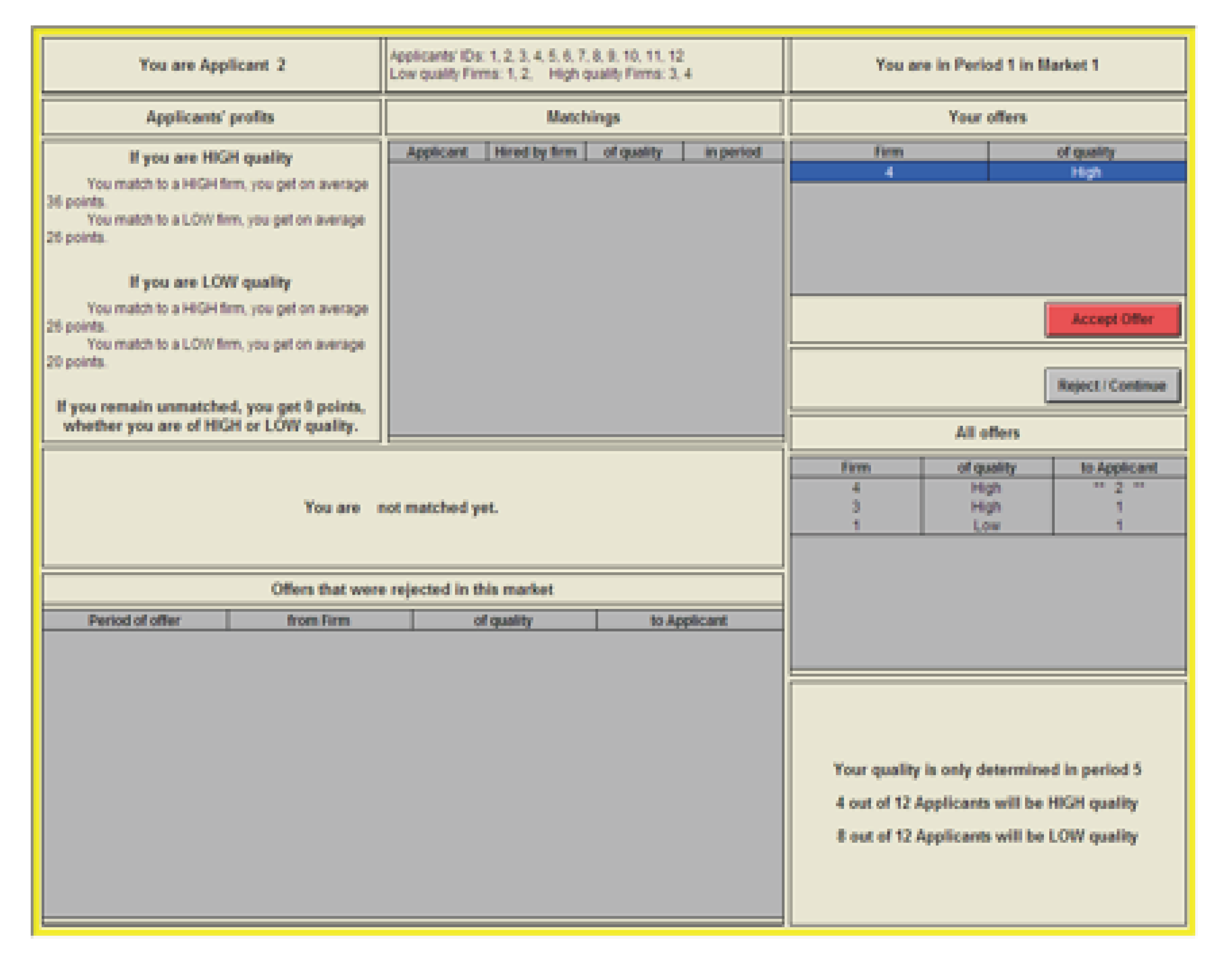
The Information on the Screen of Applicants and Firms:

In the top left box you can see whether you are a firm or an applicant. Let’s start by looking at a sample screen for one of the firms.

The Information on the Screen of Firms:

We are looking at a screen of Firm 1 (see Figure 5).
In the top right you can see the current period in the market. Each market has 8 periods, and quality information about the applicants, fit scores of applicants and firms become available in period 5. Any firm (and applicant) who is not matched by the end of period 8, remains unmatched in this market, and earns zero points. The screen shot is from period 1 of Market 1.
Below the top row, the screen is divided into two, showing the matchings that occurred in the market so far on the left and list of applicants on the right.
In the middle left, there is a box which shows whether the firm has already hired an applicant.
In the bottom left the firm has a box that records ALL offers that were rejected in this market. It shows the period in which the offer was made, which applicant received (and rejected) that offer and the ID and quality of the firm who made the offer.
All the boxes we discussed so far are also available on the screen of the applicants. Now we discuss the part that is specific to firms.
In the middle right, the firm has a box in which the firm can choose to make an offer. To make an offer, the firm types in the ID of the applicant to whom the offer is directed. To make the offer the firm has to click the “ make offer” button. The firm cannot make an offer to an applicant who is already matched to another firm.
If the firm does not want to make an offer, or is already matched, the firm has to click the “ Make No Offer” button so the experiment can proceed. (Don’t forget, since everyone has to wait until everyone has clicked a button.)
In the bottom right, there are two boxes which remind when the applicant qualities are determined (in period 5) and how many of the applicant will be HIGH quality and LOW quality (4 of them will be HIGH quality, 8 of them will be LOW quality). The second box in the bottom right, reminds the firm how many points he will get ON AVERAGE in case he hires an applicant who eventually becomes LOW quality or HIGH quality.

Firm screen: Period 5–8
The screen of the firms and applicants changes slightly beginning from period 5 (see Figure 6).
In this period, qualities of applicants, and fit scores of firms and applicants are determined. Let’s look at the screen of the same firm 1 in period 5 of the same market:
There are two changes on the screen:
The “ Matchings” box is now located on the bottom right of the screen.
The new “ List of Firms” box orders the firms by quality and fit score, the first column shows the ID numbers of firms, the second column shows their qualities, HIGH or LOW. This screen belongs to Firm 1, this is denoted by ** 1 ** in the first column instead of just 1. The third column in the box, titled “ fit” shows the fit scores of the firms. For example the best firm in this market is Firm 4 with 1.2 fit score, who is HIGH quality and has the highest fit score among HIGH quality firms while the worst firm is Firm 2 with -1.2 fit score who is LOW quality and has the lowest fit score among LOW quality firms. Note that HIGH quality firms are always better than LOW quality firms regardless of their fit scores. The fourth and fifth columns show whether firms have already hired an applicant, and if so, the ID and quality of the applicant. This screen shows that, by period 5, firm 4 has already hired applicant 2 who turned out (in period 5) to be of HIGH quality.
Figure 6. Firm Screen, Periods 5–8
Games 04 00243 g006
In the “ List of Applicants” box: the first column shows the ID numbers of applicants, the second column shows their quality, HIGH or LOW, and the third column shows their fit score. Both the quality of the applicants, and their fit score are only determined in period 5. For example the best applicant in this market is Applicant 11 of HIGH quality with 1.2 fit, while the worst applicant is Applicant 8 of LOW quality with -1.4 fit. Note that HIGH quality applicants are always better than LOW quality applicants regardless of their fit scores. The fourth and fifth columns show whether applicants were hired by a firm, and if so, the ID and quality of the firm.
The box in the middle left shows whether the firm has already hired an applicant, and if so his exact earnings. If, for example Firm 1 of LOW quality hires applicant 11 of HIGH quality with fit score 1.2, firm 1 would earn 26 points for a LOW-HIGH match, plus the applicant’s fit score of 1.2. Therefore, Firm 1’s profits would be 26+1.2=27.2 points.

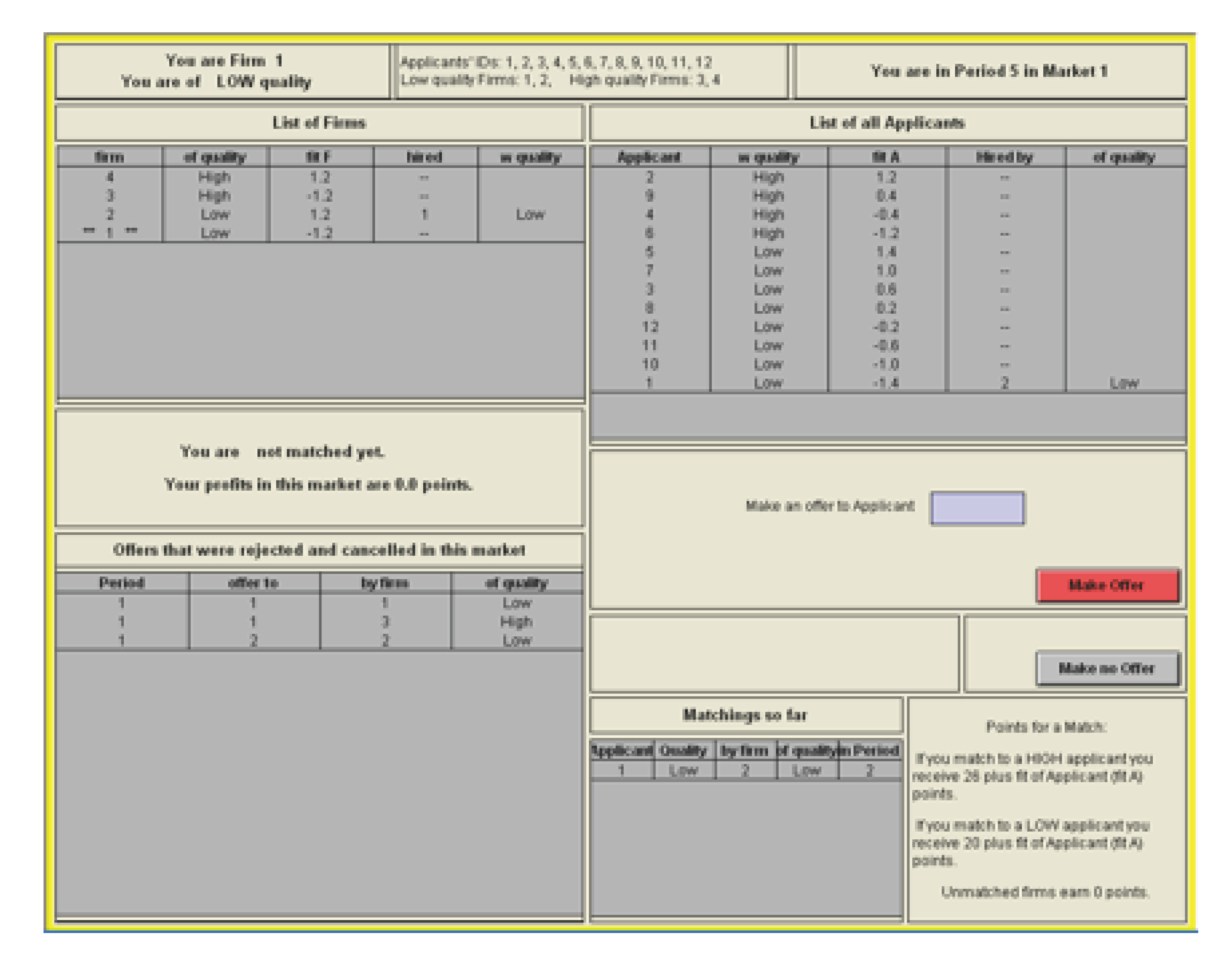
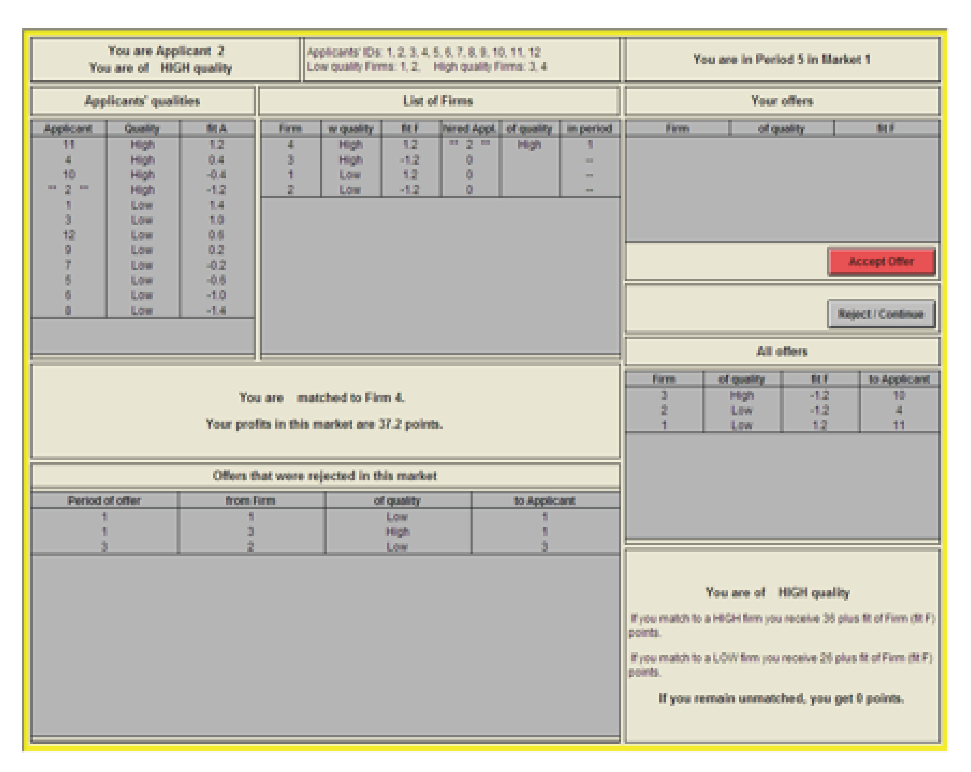
The Information on the Screen of Applicants:

This screen shot is from Applicant 2 in period 1 of Market 1 (as can be seen in the top 2 boxes) (See Figure 7).
Each applicant will receive a new ID number in every market, which has nothing to do with the final quality that is determined during the market.
Figure 7. Applicant Screen, Periods 1–4
Games 04 00243 g007
The “ Applicants’ profits” box lists the average earnings of applicants in each case when they turn out to be HIGH quality or LOW quality when they get matched to a HIGH quality firm or LOW quality firm. “ Matchings” box to the right of the above table lists who got matched to which firm in which period.
In the bottom left, the applicant has a box that reminds the applicant of ALL offers that were rejected in this market. It shows the period in which the offer was made, the ID and quality of the firm who made the offer and the ID of the applicant who received (and rejected) that offer.
Now we discuss the tables and choices that are only available to the applicants.
On the right side the applicant has a table called “ Your offers” that shows all the offers available (for this applicant). In the example, applicant 2 has one offer, from Firm 4. To accept an offer, the applicant has to first click on the offer (in this example the offer is highlighted, because it is clicked) and then click on the “ Accept offer” button. Once an applicant accepted an offer, he is matched to that firm (i.e., hired by that firm) for this market, and will not receive any subsequent offers. The applicant can also decide to reject all offers by clicking the “ Reject / Continue” button. If the applicant received no offers, he nevertheless has to click the “ Reject / Continue” button so the experiment can proceed. (Don’t forget, since everyone has to wait until everyone has clicked a button.)
The applicant not only sees his own offers but also current offers of all other applicants. Below the offers box, each applicant can see all offers made to the applicants in the current period. There are 2 other offers made in the current period in this example.
The table in the middle left shows whether and to whom the applicant is matched. And the payoff he earns in this market. Applicant 2 is not matched with any firm yet.
Figure 8. Applicant Screen, Periods 5–8
Games 04 00243 g008
The box at the bottom right is a reminder to how qualities of the applicants are determined in period 5.

Applicant screen: Periods 5–8:
The screen of applicants also slightly changes starting from period 5, when the qualities of applicants and fit scores are determined (see Figure 8).
Now the top left box tells the quality of the applicant, which is HIGH quality.
There are three changes on the applicants’ screens.
The top left “ Applicants’ qualities” box lists for each applicant, ID number, quality and fit score, where the applicants’ own ID number is marked with asterisks ** 2 ** in applicant 2’s screen shot. Notice that applicants are listed according to their qualities and then according to their fit scores, starting in period 5.
Applicant 2 turns out to have HIGH quality and the least desirable HIGH quality applicant because he has the lowest fit score among all HIGH quality applicants; he is listed 4th from the top. Applicant 8 is the worst applicant, with a LOW quality and the lowest fit score of -1.4, Applicant 11 is best applicant, with a HIGH quality and the highest fit score of 1.2.
A new box called the “ List of Firms” sorts firms according to their qualities and then according to their fit scores. Also it shows whether the firms have already hired applicants, and if so which applicants with which quality and in which period.
Finally, a box on the bottom right reminds applicants how profits are determined.
For example Applicant 2 is already hired by Firm 4 of HIGH quality with a fit score of 1.2. Applicant 2 earned on average 36 points, for a HIGH-HIGH match plus the fit score of firm 4 which is 1.2. Applicant 3 earns exactly 36+1.2=37.2 points.

Payment

The payment you receive in this experiment has two components.
The first is based on your performance in the experiment: For each point you accumulate in the experiment, you receive $0.05 (i.e., 20 points are worth $1). The second component is independent of your performance in the experiment, and already determined in advance. It consists of the $10 show-up fee. The third component is a payment of $5 that will be paid to some of the participants at the end of the experiment. The participants who will get this $5 additional payment will be announced at the end of today’s session. Your behavior in the experiment influences your payoff only through the points you accumulate in the markets (the first component of your payoffs). Your total payment will be rounded to the nearest dollar.

Summary

At the beginning of the experiment you learn whether you are a firm or an applicant. If you are a firm, you also learn your quality, which is LOW for firms 1 and 2 and HIGH for firms 3 and 4. Your ID number has however nothing to do with your fit score. If you are an applicant, you receive a new ID number in every market, and your ID number has nothing to do with both your quality and your fit score. In each market there are 4 firms and 12 applicants.
Information about Applicants’ qualities is revealed over periods:
  • Periods 1–4: Each applicant has equal chance to be a HIGH quality applicant (4 of the 12 that is 1 in 3 applicants will be of HIGH quality) and equal chance to be a LOW quality applicant (8 of the 12 that is 2 in 3 applicants will be of LOW quality).
  • Periods 5–8: At the beginning of period 5, four applicants become HIGH quality and the remaining eight applicants become LOW quality applicants.
  • Periods 5–8: Firms and applicants are assigned small fit scores. A HIGH quality partner with the lowest fit is still much more desirable than a LOW quality partner with the highest fit. But the higher the fit score, the more desirable that partner is.
To earn points in a market, a firm will need to hire one, and only one, applicant in that market, and an “ applicant” will need to accept one, and only one, job offer. How is this done?
  • In each period, each firm that has not yet hired an applicant, has to decide whether to make an offer and, if so, to which applicant. Each firm can only make one offer in each period, and only to applicants who have not accepted an offer yet.
  • In each period, applicants who receive offers have to decide whether to accept or reject the offer.
  • Once an applicant accepted an offer, he cannot accept another offer in the same market, and will no longer receive offers.
  • Firms and Applicants that are not matched by the end of period 8 in a market remain unmatched and earn zero points.
  • In a HIGH quality-HIGH quality match, firms and applicants each earn 36 points plus the fit scores of their partner.
  • In a HIGH quality-LOW quality match, firms and applicants each earn 26 points plus the fit scores of their partner.
  • In a LOW quality-LOW quality match, firms and applicants each earn 20 points plus the fit scores of their partner.
  • After period 8, a completely new market begins, and everyone is free to try to match once again.
  • The experiment has 20 consecutive markets each with 8 periods length.
On a technical note: The applicant screen only comes up when all firms made a decision, that is, as soon as applicants see their screen, they can make decisions right away, as the information on their screen will not change over time. If applicants received no offer, or firms are already matched in a market, please hit the Continue button right away to speed up the experiment.

