Bimodal Bidding in Experimental All-Pay Auctions

Abstract

We report results from experimental first-price, sealed-bid, all-pay auctions for a good with a common and known value. We observe bidding strategies in groups of two and three bidders and under two extreme information conditions. As predicted by the Nash equilibrium, subjects use mixed strategies. In contrast to the prediction under standard assumptions, bids are drawn from a bimodal distribution: very high and very low bids are much more frequent than intermediate bids. Standard risk preferences cannot account for our results. Bidding behavior is, however, consistent with the predictions of a model with reference dependent preferences as proposed by the prospect theory.

1. Introduction

Bidding behavior in all-pay auctions has so far only received limited attention in empirical auction research. This might be due to the fact that most of the applications of auction theory do not involve the all-pay rule. However, occurrences of this auction format, where every bidder pays her bid are numerous: lobbying battles, political campaigns, promotion tournaments in firms and applications for science grants [1].

In this article, we report experimental data on bidding behavior from the simplest possible all-pay auction format. We conducted first-price, sealed-bid, common value auctions with two or three subjects and no uncertainty with regard to the value of the auctioned commodity. Every subject bids in an auction for a prize of 100 monetary units. Subjects choose their bids simultaneously, the highest bidder receives the prize, and all bidders pay their bid. In this game only mixed-strategy equilibria exist. While the hitherto existing literature on this auction format focuses on average outcomes, we concentrate on the distribution of bids. We analyze bidding behavior in ten subsequent auctions and under two information conditions. In the NoRecall treatment subjects do not receive any information about other subjects’ bids during the ten rounds and they are randomly rematched every round to a group of two or three players. In the Recall treatment subjects are matched into stable groups and have full information about the bidding history in their group. The two treatments differ in more than one dimension. The key idea is not to identify a causal effect of a single design feature, but to observe bidding strategies under two very different information conditions. In Recall it is highly salient that players’ actions should not be predictable. We expect this to be the condition most favorable for observing mixed strategies. On the other hand, in NoRecall players know that their competitors remain uninformed about their actions, so predictability of future bids from observed past bids is not an issue. Even if they play a mixed strategy, it is not clear whether they would draw their bid from the density only once or redraw a bid in every period.

In both treatments we find that subjects indeed use mixed strategies, however, the observed distribution of bids shows interesting deviations from the predictions under standard assumptions. The mixed strategy Nash equilibrium under standard assumptions predicts uniformly distributed bids for groups of two players and a decreasing density function for larger group sizes. We find that subjects’ bidding strategies differ sharply from these predictions: on average, subjects apply bimodal bidding strategies which give most weight to both very low and very high bids, resulting in a bimodal bidding function. Bimodal bidding occurs for both group sizes and information conditions. We show that bimodal bidding is consistent with prospect theory. If players are risk seeking in the domain of losses and risk averse in the domain of gains, then equilibrium bidding strategies are bimodal.

Previous evidence on bidding behavior in experimental all-pay auctions comes from Gneezy and Smorodinsky [2], who conducted similar all-pay auctions as we do with group sizes of four to twelve and focus on the effect of different group sizes on the auctioneers’ revenue. They report persistent overbidding, i.e., average bids were considerably higher than predicted by the Nash equilibrium for all group sizes.1 Müller and Schotter [6] examine four player contest games where players have private information about their abilities. This setup allows for Nash equilibria in pure strategies where optimal bids (efforts) are continuously related to ability. The data shows, however, that observed efforts bifurcate, i.e., subjects seem to play a threshold strategy of choosing either high effort or no effort at all. We observe a similar effect in a much simpler setup under perfect information. Both Müller and Schotter’s and our data are compatible with Prospect theory preferences. In Section 2 we present the theory and our experimental design. Section 3 presents the results and Section 4 discusses potential explanations for the bimodal bidding strategies observed in the experiment.

2. Theory and Experimental Design

The game is played in groups of n = 2 or 3 bidders. All players choose their bid simultaneously. The auctioned commodity has a value of unity for all bidders. A player’s expected utility is defined as:

(1)

M(b^max)counts the number of maximal bidders. Following this, we intuitively derive the Nash equilibria of this game assuming risk neutrality (this assumption is relaxed in Section 4). A thorough theoretical treatment of this game is provided by Baye et al. [7]. Clearly the game cannot have an equilibrium in pure strategies because the best reply to every bid in [0,1) is to overbid by the smallest amount possible. In every mixed strategy equilibrium it must hold that bidders are indifferent between the mixed strategy and any pure strategy included in their mixed strategy. As long as the support of the mixed strategy includes zero, the expected utility in the mixed strategy must be zero. For n = 2 this game has a unique equilibrium in mixed strategies where both players draw their bid from a uniform distribution over the support [0,1]. The expected utility then equals zero for both players.

Could the two players improve their situation by restraining the support of their mixed strategy from above, i.e., both drawing their bid from [0, b] with b < 1? No, because this would offer the opportunity of earning a strictly positive payoff by outbidding the other player with a pure strategy of bidding slightly more than b. Could they improve by choosing their bid from [b, 1] with b > 0? This is also not possible as bidding b would then result in a certain loss and the player would prefer to bid 0. To conclude, both players choose their bid from a uniform distribution with support [0,1] and earn an expected payoff of zero. Expected bids are 0.5 and expected standard deviation is . Expected gross return of the auctioneer is 1, which equals the value of the auctioned commodity.

For n = 3 the theoretical solution becomes more complicated. There exists a unique symmetric equilibrium where all players draw their bid from a distribution with density f (b_i) = 0.5b_i^-0.5, b_i ∈ [0,1]. In addition, there is a continuum of equilibria of the following kind: two players randomize on [0,1] while the third player randomizes continuously on an interval [b, 1] and concentrates the remaining mass at zero, with 0 ≤ b ≤ 1. The equilibria reach from b = 0, which is the symmetric case to b = 1, in which the third player does not take part in the auction and the other two players choose their bids according to the equilibrium strategy in the two player case. Expected bids for the two players who randomize with full support range from one third to one half, expected bids from the third bidder range from zero to one third. All equilibria share the following features: the expected bids are one third, expected utility of all bidders is zero and the revenue for the auctioneer is unity. Standard deviations of the bids depend on the equilibrium and range from 0.298 for b = 0 to 0.333 for b = 1.

We conducted two treatments, the Recall and the NoRecall treatment. In the Recall treatment subjects were allocated to groups of either two or three subjects and played ten consecutive but independent all-pay auctions for a prize of 100 ECU (experimental currency unit) in a partner matching.2 Full information about bids of group members in all previous rounds was provided. In the NoRecall treatment subjects also played ten consecutive all-pay auctions for a prize of 100 ECU. In the latter we use a stranger matching, i.e., in each round subjects were randomly reallocated to groups of either two or three subjects. They were informed about their group size but received no information at all about the outcome of the auction and the other subjects’ bids.

Our experimental subjects were first year students from the University of St. Gallen. Subjects did not have prior knowledge in game-theory and had not participated in auction experiments before. The experiment was programmed and conducted with the software z-Tree [8]. Prior to the experiment subjects were given detailed instructions (see appendix). Bids were restricted to the interval [0,125] and a resolution up to three decimal places.3 At the beginning of the experiment subjects received a show-up fee of CHF 20 (about USD 20). Losses in the experiment were deducted from the show-up fee. The auctioned item was 100 ECU (which corresponded to CHF 1, about $1). We report results from 52 subjects in two sessions. We apply a within subject design where all subjects played both the Recall and NoRecall treatment, changing the order of the treatments between the sessions. In Recall we observe 14 (8) independent groups with n = 2 (3), in NoRecall all 28 subjects which played this treatment first are independent (due to the lack of feedback). The observations of NoRecall played as second treatment are dependent within group from the Recall treatment, which results in 10 independent groups. The experiment lasted about an hour and the subjects earned an average of CHF 19.4 (about $19.5), which means that, on average, subjects made a small loss of CHF 0.6 in the 20 auctions they played.

3. Results

We start by analyzing the data from the Recall treatment.4 In this treatment subjects had access to the whole history of bids within their group and played the game in stable groups. These are arguably the conditions most favorable for the establishment of a mixed-strategy equilibrium. Average bids over the ten rounds were 42.0 in groups of two and 36.9 in groups of three. Compared to the Nash prediction of 50 and 33.3 respectively, we observe underbidding in groups of two and overbidding in groups of three. The differences are, however, not significant.5 We do not observe convergence towards the Nash equilibrium over the course of the ten periods.6 Average bids are, however, not very informative when it comes to the bidding strategies subjects played. If we calculate the standard deviation of the bids, we observe 40.0 in groups of two which is higher than predicted by the Nash equilibrium (28.9). In groups of three, the observed standard deviation was 39.8 compared to the prediction which lies between 29.8 and 33.3.7

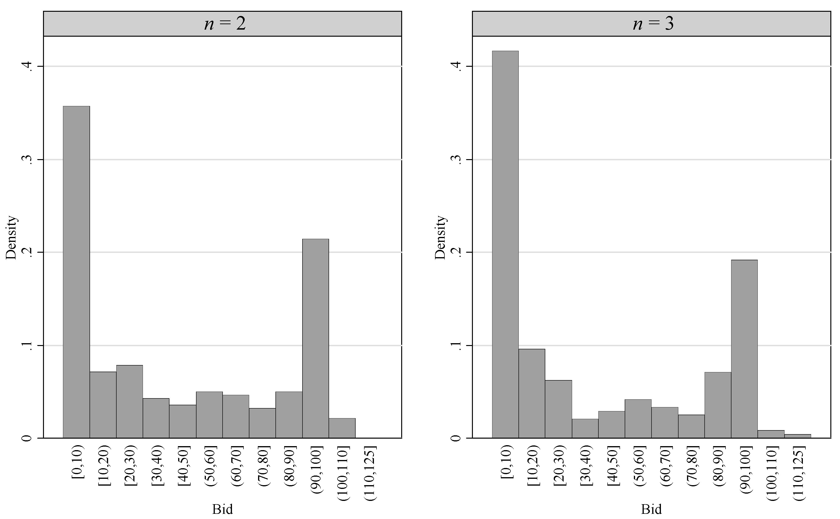
Striking differences to the Nash equilibrium under standard assumptions emerge if we take a closer look at the distribution of bids. Figure 1 shows histograms of the bids separated by group size. For both group sizes the distribution of bids is clearly bimodal. Very low and very high bids (up to 100) are much more frequent than intermediate bids.

Figure 1. Histogram of bids in groups of two and three subjects in the Recall treatment.

Figure 1. Histogram of bids in groups of two and three subjects in the Recall treatment.

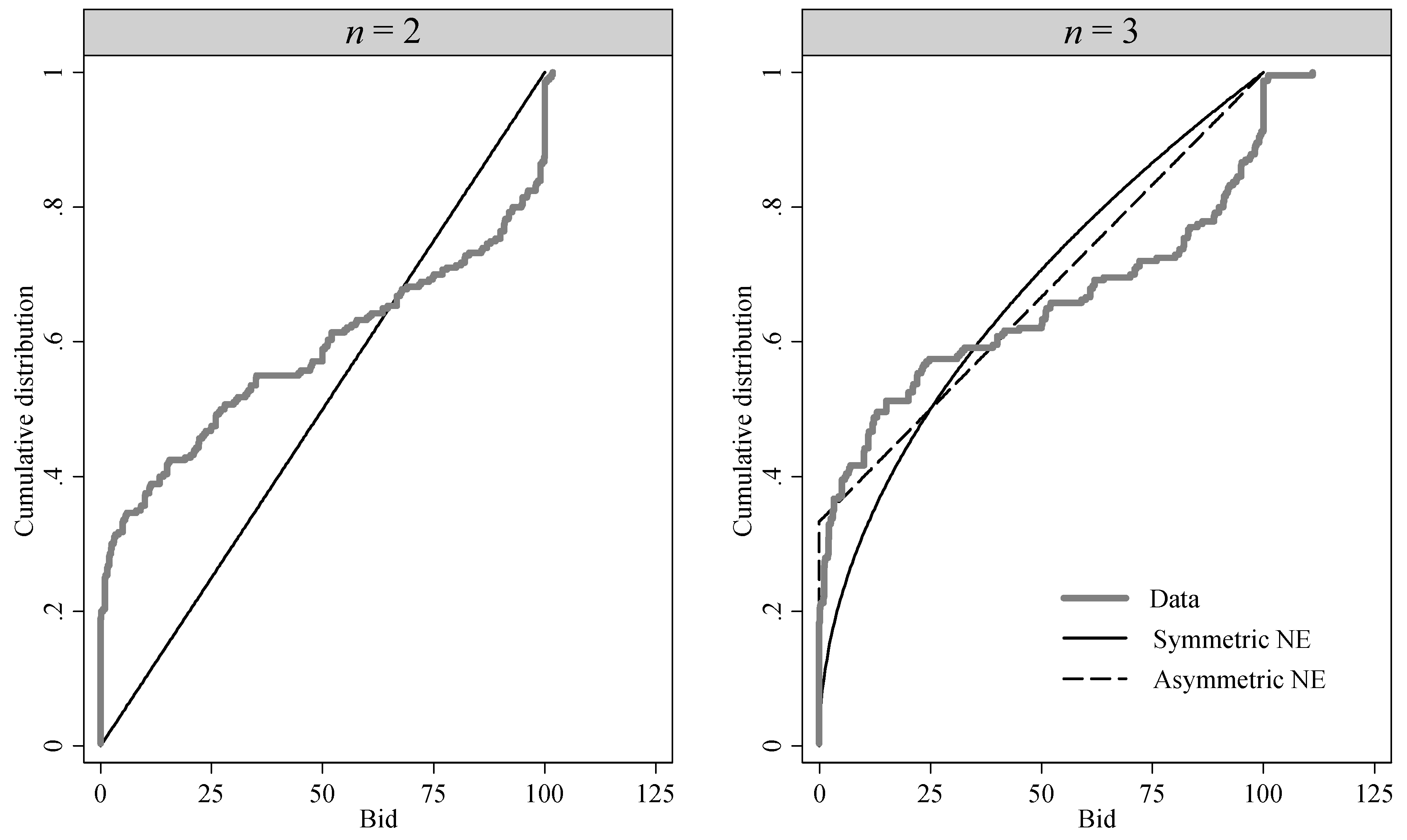
To facilitate the comparison between observed and predicted bids, Figure 2 shows the cumulative distribution of the observed bids (bold lines) and the cumulative densities of the Nash equilibria (thin lines). In the right panel we account for the fact that multiple equilibria exist and depict the cumulative densities of the two most extreme cases: The thin kinked curve corresponds to the equilibrium where one player abstains from the auction (hence the intercept at one third) and the other two players draw their bid from a uniform distribution; the smooth thin curve corresponds to the symmetric mixed strategy equilibrium.

For the smaller group size, prediction and data are obviously very different. In the auctions with three bidders, the large mass at very low bids is compatible with an asymmetric mixed strategy equilibrium. Still, the mass of bids close to 100 is clearly incompatible with the prediction. If we apply Kolmogorov-Smirnov tests for the null hypothesis that the bids stem from the predicted densities we can reject the null hypotheses for both group sizes and all equilibria at p < 0.001.8

Figure 2. Nash equilibrium (thin lines) and observed cumulative distribution functions of bids by group size in the Recall treatment (bold lines).

Figure 2. Nash equilibrium (thin lines) and observed cumulative distribution functions of bids by group size in the Recall treatment (bold lines).

3.1. Group and Individual Bidding Behavior

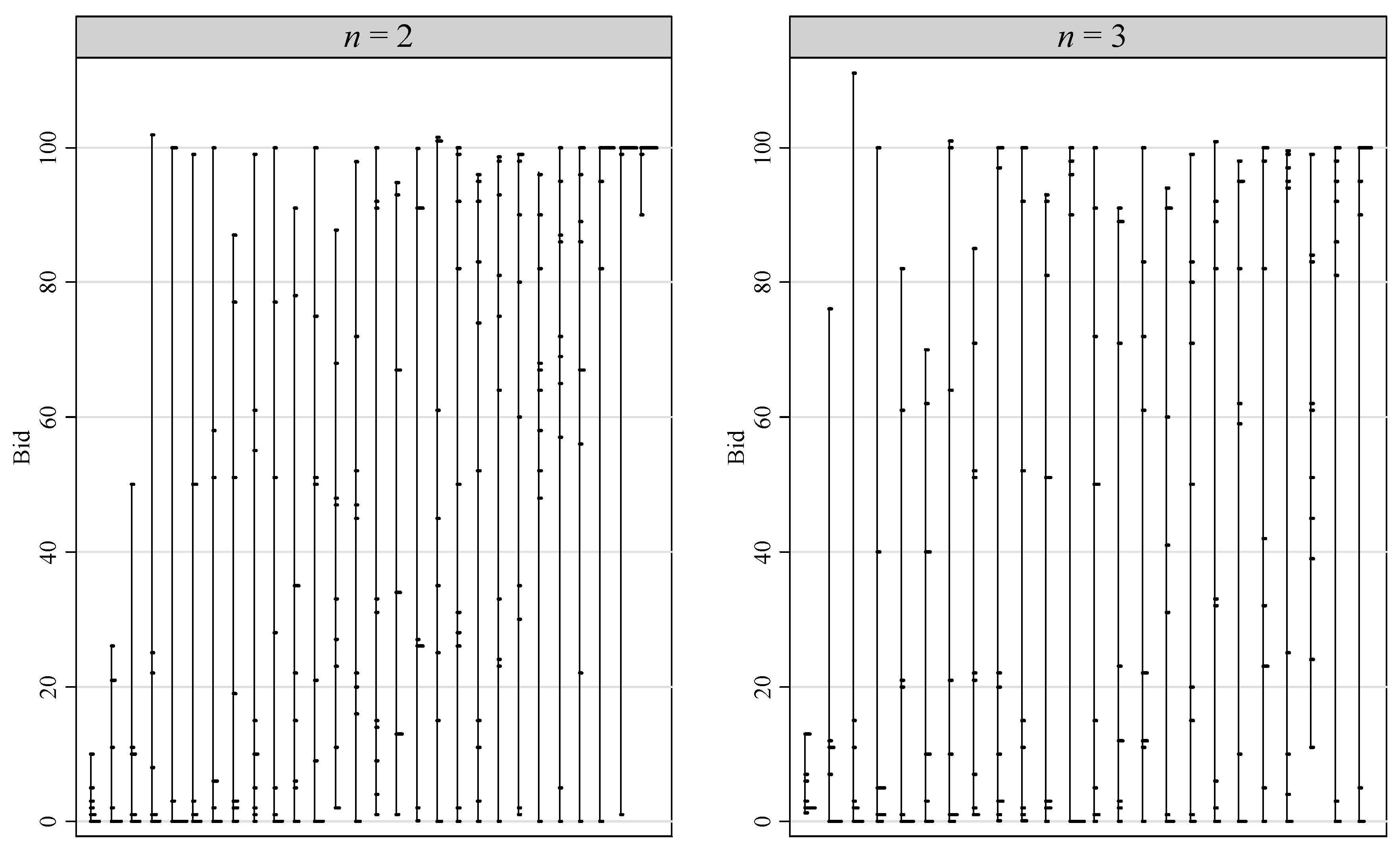
In a next step, we will look at group differences and individual patterns. For groups of two bidders we observe a wide variety of outcomes, ranging from average bids of 5.2 to 93.3 over the ten periods. There is a cluster of five groups at around 25 while the majority of groups are located between 40 and 55. The standard deviation of the average group bids is 22.1. For groups of three we observe less variation with average group bids ranging from 21.8 to 47.3 and a standard deviation of 8.5. Figure 3 depicts small histograms for individual bidding behavior over the ten rounds of the Recall treatment, for both group sizes. Each vertical line corresponds to one subject in the experiment and shows the spread of the bids. Subjects are sorted according to average bid. The length of the small horizontal spikes corresponds to the frequency of the corresponding bid (bids are rounded to integers). The overwhelming majority of the subjects bid in the entire range from zero to (almost) 100. Three quarter of the subjects have a spread of 90 or more in their ten bids. The majority of the subjects changed their bid frequently during the ten rounds. If we calculate the number of different bids a subject chose, we obtain an average of 7.96 different bids in the 10 auctions. More than a quarter of the subjects chose different bids in all ten rounds. We can also look at the number of changes in a subject’s bid from one round to the next. In 90.4 percent of the cases subjects changed their bid from t to t + 1.9

Figure 3. Individual histograms of the bids in the ten rounds of the Recall treatment.

Figure 3. Individual histograms of the bids in the ten rounds of the Recall treatment.

Note: Vertical lines show the spread of the bids of each individual, small horizontal lines depict the frequency of the corresponding bid (bids are rounded to integers).

3.2. Reducing Information

Thus far we have only analyzed data from the Recall treatments, where subjects learn of other subjects’ bids and can react to this information in subsequent rounds. In the NoRecall treatments subjects receive no feedback at all from the game and cannot find out the success of their strategies. In such a game it is even more difficult to infer a subject’s bidding strategy from the observed bids. Even if subjects play a mixed strategy, in the sense that they use a random draw from a probability distribution to determine their bid, it is unclear whether they draw every round or only once at the beginning of the experiment (possibly for each group size).

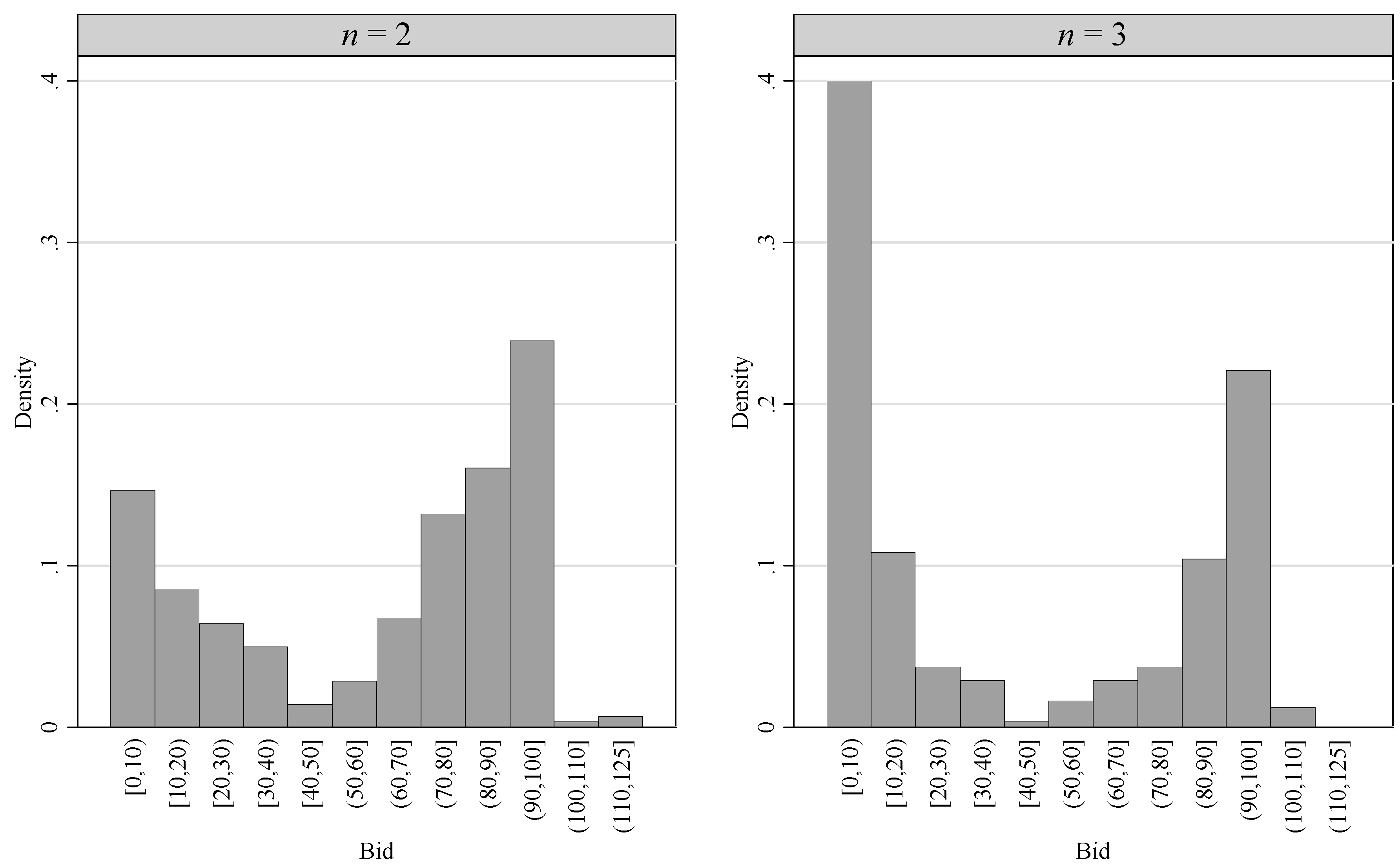
Average bids (standard deviation) in NoRecall are 59.5 (36.1) and 41.2 (41.9) for groups of two and three subjects respectively. For both group sizes bids are higher than the Nash prediction.10 On the individual level we observe that subjects changed their bids less frequently in the NoRecall treatment compared to the Recall treatment, despite the fact that in the NoRecall treatment group size changed over time. During the ten rounds, subjects chose an average of 6.60 different bids (as opposed to 7.96 in the Recall treatment). Still, the overall distribution of bids was clearly bimodal for both groups of two and three subjects. Figure 4 shows histograms for the bids in the NoRecall treatments.

Figure 4. Histogram of bids in groups of two and three subjects in the NoRecall treatment.

Figure 4. Histogram of bids in groups of two and three subjects in the NoRecall treatment.

4. Why Bimodal Bidding?

Why should one adopt a bimodal bidding strategy? Recall that the theoretical prediction derived in Section 2 assumed risk neutral bidders. It is thus natural to explore the game theoretic predictions under different assumptions with regard to the utility function. Let us consider an arbitrary utility function u( x_i ) where x_i is the monetary payoff and u′ > 0. For every mixed-strategy equilibrium with n homogeneous players it must hold that:

(2)

The expected utility of every bid b_i used in the strategy equals the probability of winning the auction times the utility in case of a win, plus the probability of losing the auction times the respective utility. Both terms depend on F( ), which is the cumulative density of the bidding strategy of the other bidders. For a mixed strategy with full support to be a best reply, this expression must be constant and equal to the utility of bidding zero. Following we assume u(0) = 0 without loss of generality. Thus, the utility of winning the auction will be positive and losing the auction will yield zero or negative utility. From this expression we can easily derive the cumulative density of the equilibrium bidding strategy with arbitrary (but symmetric) utility functions as:

(3)

What densities f (b_i) can we generate with standard risk preferences?11 If we introduce different risk preferences into the utility function using a function with hyperbolic absolute risk aversion, we can only predict unimodal bidding strategies in groups of two players. Relative to the risk neutral case, risk aversion shifts mass towards low bids while risk seeking preferences shift mass towards high bids.12

It turns out that the bidding strategies observed in our experiment can be explained by the curvature of the utility function if we allow for concave and convex regions, like in Kahneman and Tversky’s [10] prospect theory. A core element of prospect theory is that players evaluate their outcome relative to a reference point. If they earn more than their reference point, they are in the domain of gains, otherwise in the domain of losses. Kahneman and Tversky propose a ‘value function’ that is concave in the domain of gains and convex in the domain of losses. In addition to that, Kahneman and Tversky introduce a ‘loss aversion’ parameter, which incorporates the notion that most people suffer more from the loss of a certain amount of money than they enjoy the win of the same amount. For illustration purposes we use the parametric specification proposed in Tversky and Kahneman [11]:

(4)

We denote the amount of money a player earns in an auction by x; α is a parameter for the curvature of the value function. Risk aversion in gains and risk seeking in losses requires 0 < α < 1; λ is a shifting parameter in the domain of losses, which is larger than one for loss aversion. We assume that in every auction the reference point is the actual wealth when entering the auction. Thus, winning the auction with a bid below 100 puts a player in the domain of gains while losing the auction with a positive bid puts a player in the domain of losses.13 A second integral part of prospect theory is the probability weighting function which maps objective probabilities into subjective probabilities. For simplicity we do not consider the probability weighting function in our context because, unlike in the typical application of prospect theory, subjects in our game do not know the probability of winning and losing.14

Substituting Equation (4) into (3) and replacing u(–b_i) by –λ(b_i) ^α and u(1 – b_i) by (1 – b_i) ^α we get the predicted cumulative density. The first order derivative gives us the mixed-strategy density function for prospect theory players. We use maximum likelihood to estimate the preference parameters α and λ from the bids observed in the experiment. The log likelihood is

(5)

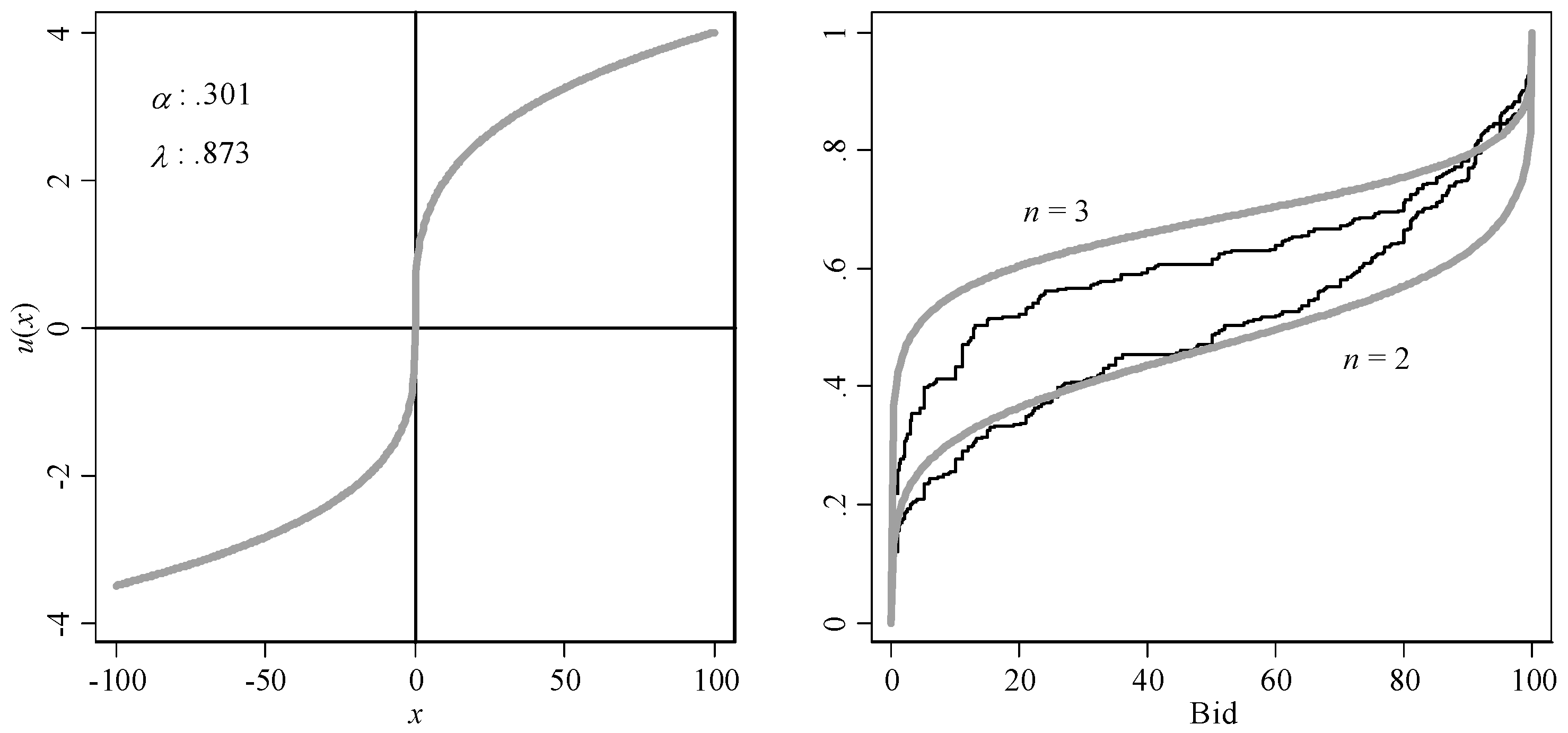
Because the theoretical solution is the same for both treatments, we pool the data from the Recall and NoRecall treatments. The estimates for the preference parameters are α = 0.301 (se: 0.032), and λ = 0.873 (se: 0.095).15,16 The left panel in Figure 5 depicts the value function. The right panel depicts the fitted cumulative densities and the observed bids.

Figure 5. Left panel: Prospect theory value function with estimated parameters. Right panel: Observed (bold lines) and predicted (thin lines) cumulative densities for both group sizes.

Figure 5. Left panel: Prospect theory value function with estimated parameters. Right panel: Observed (bold lines) and predicted (thin lines) cumulative densities for both group sizes.

Figure 5 shows that the combination of risk aversion in the domain of gains and risk seeking behavior in the domain of losses as proposed by Kahneman and Tversky [10] can account for bimodal bidding behavior.17 Intuitively the subjects use a make-or-break strategy, i.e., they either submit a very low bid and hope for the lucky punch or they submit a very high bid in order to increase the winning probability. Submitting low bids is not costly, offsetting the low winning probability. Submitting high bids increases the winning chances but also the amount to lose. The potentially high loss connected with this strategy is acceptable due to the risk seeking preferences in the domain of losses.

Surprisingly, the point estimate for the loss aversion parameter λ is smaller than one, which means the opposite of loss aversion, i.e., some sort of loss tolerance.18 This is at odds with many observations from experiments on loss aversion in risky choice situations, which find values above one (see e.g., Gächter et al., [16] or Abdellaoui et al. [17]). We think that the main difference between this existing literature and our results is that we observe risky choices in a strategic situation with competitive characteristics.19 We speculate that there is a preference for competing, which makes winning in an auction more attractive than earning the same amount of money from a ‘simple’ lottery. This is consistent with the frequently found excessive entry or bidding behavior in market entry games, contests, and auctions (e.g., Fischbacher and Thöni [18]; Sheremeta [19]; Cooper and Fang [20]). We could enrich the utility function with an additional parameter measuring the joy of winning the auction, like e.g., multiplying the upper part of Equation (4) with some parameter v (for victory). However, our data does not allow identifying v independently from λ and we have to leave this question for future research.

Prospect theory can account for bimodal bidding and for the fact that mass is shifted from the higher mode to the lower mode of the distribution when the number of contestants in the auction increases. This corresponds to the observations in our experiment and also to the data reported by Gneezy and Smorodinsky [2]. Furthermore, by allowing a λ lower than one, we can account for the fact that in larger groups bids are typically higher than predicted by the Nash equilibrium under standard assumptions.

5. Conclusions

We investigated bidding strategies in very simple common value all-pay auctions with no pure strategy equilibria. Bidders in our experiment use bimodal, mixed strategies that are remarkably different from the mixed strategies predicted by the Nash equilibrium under standard assumptions. Bimodal bidding strategies are observed under two very distinct information conditions: They occur in Recall, where bidders are in stable groups with full information about the bidding history, as well as in NoRecall, where bidders do not receive any information about other bidders’ strategies.

The bimodality in the distribution of bids cannot be explained by standard risk preferences but fits very well to the S-shaped value function proposed by Kahneman and Tversky’s [10] prospect theory. We use our data to estimate preference parameters. For the curvature of the value function, our parameter estimates are comparable to the ones reported in previous literature. For the second ingredient of the prospect theory’s value function—loss aversion—we find different results. The observed bidding strategies are best explained when assuming the contrary of loss aversion. The reason for this is presumably not because our subjects like losses, but because the competitive structure of the game offers them additional utility when winning the auction.

This hypothesized additional utility for winning an auction can also explain why bids tend to become excessive in larger groups, leading to systematic losses for the bidders in such all-pay auctions. Anderson et al. [21] propose the logit equilibrium as a solution concept to account for excessive bids. In this framework players are boundedly rational in the sense that they make random errors when choosing their bid. The probability of choosing a strategy that is not a best reply is negatively related to the expected payoff of that strategy. The distribution of bids we observe in our data makes this explanation highly unlikely, as a bimodal distribution of bids is not compatible with this kind of erroneous bids. Errors simply shift the densities predicted by the Nash equilibrium under standard assumptions towards the uniform distribution, but cannot produce a second mode at high bids.

Many competitive situations in the real world involve aspects of all-pay auctions, like lobbying battles, competing for research money and so on. In small groups we find that average bids are relatively close to the Nash equilibrium under standard assumptions but the distribution of bids is strikingly different. In accordance to what Müller and Schotter [6] report for contest games we find that the average subject employs an ‘all-or-nothing’ strategy, i.e., either goes for a lucky punch with a small bid or tries to ensure winning the auction with a very large bid. A rational bidder seeking to maximize monetary payoff should therefore always bid slightly above the lower mode. With our data this would have corresponded to a bid of 6.10 for groups of two and 13.10 for groups of three subjects.

Our results provide evidence for predictive power of models of reference dependent preferences such as prospect theory in a highly competitive environment. In line with Müller and Schotter [6], but, in a much simpler game, we show that the notion of risk aversion in the domain of gains, and risk seeking behavior in the domain of losses, predicts mixed strategies more accurately than the standard expected utility theory.

References

- Klemperer, P. Auctions: Theory and Practice; Princeton University Press: Princeton, NJ, USA, 2004. [Google Scholar]
- Gneezy, U.; Smorodinsky, R. All-pay auctions—an experimental study. J. Econ. Behav. Organ. 2006, 61, 255–275. [Google Scholar] [CrossRef]
- Noussair, C.; Silver, J. Behavior in all-pay auctions with incomplete information. Games Econ. Behav. 2006, 55, 189–206. [Google Scholar] [CrossRef]
- Barut, Y.; Kovenock, D.; Noussair, C.N. A comparison of multiple-unit all-pay and winner-pay auctions under incomplete information. Int. Econ. Rev. 2002, 43, 675–708. [Google Scholar] [CrossRef]
- Fehr, D.; Schmid, J. Exclusion in the all-pay auction: An experimental investigation. WZB Discuss. Pap. 2010. SP II 2010-04. [Google Scholar]
- Müller, W.; Schotter, A. Workaholics and dropouts in organizations. J. Eur. Econ. Assoc. 2010, 8, 717–743. [Google Scholar]
- Baye, M.U.; Kovenock, D.; de Vries, C.G. The all-pay auction with complete information. Econ. Theory 1996, 8, 291–305. [Google Scholar]
- Fischbacher, U. z-Tree: Zurich toolbox for ready-made economic experiments. Exp. Econ. 2007, 10, 171–178. [Google Scholar] [CrossRef]
- Fibich, G.; Gavious, A.; Sela, A. All-pay auctions with risk-averse players. Int. J. Game Theory 2006, 34, 583–599. [Google Scholar] [CrossRef]
- Kahneman, D.; Tversky, A. Prospect theory: An analysis of decision under risk. Econometrica 1979, 47, 263–291. [Google Scholar] [CrossRef]
- Tversky, A.; Kahneman, D. Advances in prospect theory: Cumulative representations of uncertainty. J. Risk Uncertain. 1992, 5, 297–323. [Google Scholar] [CrossRef]
- Köszegi, B.; Rabin, M. A model of reference-dependent preferences. Q. J. Econ. 2006, 121, 1133–1165. [Google Scholar]
- Camerer, C.F.; Ho, T.-H. Violations of the betweenness axiom and nonlinearity in probabilities. J. Risk Uncertain. 1994, 8, 167–96. [Google Scholar] [CrossRef]
- Wu, G.; Gonzalez, R. Curvature of the probability weighting function. Manag. Sci. 1996, 42, 1676–1690. [Google Scholar] [CrossRef]
- Booij, A.S.; Praag, B.M.S.; van de Kuilen, G. A parametric analysis of prospect theory’s functionals for the general population. Theory Decis. 2010, 68, 115–148. [Google Scholar] [CrossRef]
- Gächter, S.; Johnson, E.J.; Herrmann, A. Individual-level loss aversion in riskless and risky choices. CeDEx Discuss. Pap. 2007. No. 2007-02. [Google Scholar]
- Abdellaoui, M.; Bleichrodt, H.; Paraschiv, C. Loss aversion under prospect theory: A parameter-free measurement. Manag. Sci. 2007, 53, 1659–1674. [Google Scholar] [CrossRef]
- Fischbacher, U.; Thöni, C. Excess entry in an experimental winner-take-all market. J.Econ. Behav. Organ. 2008, 67, 150–163. [Google Scholar] [CrossRef]
- Sheremeta, R.M. Experimental comparison of multi-stage and one-stage contests. Games Econ. Behav. 2010, 68, 731–747. [Google Scholar] [CrossRef]
- Cooper, D.J.; Fang, H. Understanding overbidding in second price auctions: An experimental study. Econ. J. 2008, 118, 1572–1595. [Google Scholar] [CrossRef]
- Anderson, S.P.; Goeree, J.K.; Holt, C.A. Rent seeking with bounded rationality: An analysis of the all-pay auction. J. Polit. Econ. 1998, 106, 828–853. [Google Scholar] [CrossRef]
Appendix: Experimental Instructions (translated from the original instructions written in German)
General Explanation for the Participants
You are now taking part in an economic experiment that is financed by different research-promoting facilities. If you read the following explanation carefully, you can—depending on your decisions—make a considerable amount of money. Hence, it is important that you read this explanation carefully.
The instructions you will receive are for your private information only.
During the Experiment Absolute Silence Is Required. Communication Is Prohibited
If you have any questions please direct them towards us. Non-observance of these rules will lead to exclusion from the experiment and any payments.
In the experiment we do not quote Swiss Francs. Your income will be calculated in points. At the end of the experiment, the attained points will be transferred into Swiss Francs, where
1 point = 1 centime.
At the end of the experiment you will receive your earned points (in CHF) plus CHF 20 for participating, in cash. If you make a loss, it will be deducted from the CHF 20. You cannot make an overall loss.
The next pages describe the detailed procedure of the experiment.
Experiment Instructions: Recall Treatment
You are taking part in an auction. In total there are 10 rounds and in each of these rounds a prize of 100 points is auctioned.
You will be put in a group of either two or three participants. Hence there will be one other or two other bidders in your group besides yourself. The group composition will remain constant during the 10 rounds, i.e., in each round you will remain in the same group with either one or two other participants. You will not know who else in this room is in your group; your identity will be kept secret. When the auction begins you will have to place your bid. All participants do so at the same time. You can place a bid up to three decimal places. In each group the participant placing the highest bid wins. If more than one participant bids the same highest value, the computer randomly assigns the winner. In contrast to normal auctions you might know, not only the winner but all bidders have to pay their bid. As soon as the experiment starts you will see the following screen:
![Games 04 00608 i007]()
On the screen, you can see whether you are placed in a group with 2 or 3 participants. In the right hand upper corner you can note the time remaining for you to place your bid. Type your bid into the field. After submitting the bid [pressing OK] you will not be able to change it again. You only bid once in each round. You can place bids from, and including, zero and up to three decimal places.
As soon as all the participants have submitted their bids, the computer will calculate the highest bid and determine the earnings in points. It will then appear on a screen showing the outcome of the auction:
![Games 04 00608 i008]()
You will be notified if you won the auction and of your revenue earned in each round. Additionally you will see the bids of the other participant(s) as well as your own. Subsequently press the ‘continue’ button to proceed to the next round.
An example to clarify the rules:
Assuming that in a group of three participants the following bids are submitted:
- 10 points
- 50 points
- 80 points
Claus wins the auction and has a revenue of 20 points (=100-80) in this round. Anton and Berta do not win, but have to pay their bid nevertheless. The revenue of Anton is therefore −10 and that of Berta is −50 in this round.
Do you have any questions?
Experiment Instructions: NoRecall Treatment
Explanation to the Second Experiment
The second experiment also consists of 10 rounds, in each of which 100 points are to be auctioned. There are two important modifications:
- You will not receive any information whether or not you won the auction in this round. You will also not receive any information about the bids of the other participants.
- The constellation of the group changes in each round. The group size varies between 2 and 3. The computer will randomly assign you in a group of 2 or of 3. You will be able to see the size on the screen.
© 2013 by the authors; licensee MDPI, Basel, Switzerland. This article is an open access article distributed under the terms and conditions of the Creative Commons Attribution license (http://creativecommons.org/licenses/by/3.0/).
Share and Cite
MDPI and ACS Style
Ernst, C.; Thöni, C. Bimodal Bidding in Experimental All-Pay Auctions. Games 2013, 4, 608-623. https://doi.org/10.3390/g4040608
AMA Style
Ernst C, Thöni C. Bimodal Bidding in Experimental All-Pay Auctions. Games. 2013; 4(4):608-623. https://doi.org/10.3390/g4040608
Chicago/Turabian StyleErnst, Christiane, and Christian Thöni. 2013. "Bimodal Bidding in Experimental All-Pay Auctions" Games 4, no. 4: 608-623. https://doi.org/10.3390/g4040608