Learning in Networks—An Experimental Study Using Stationary Concepts

Abstract

Our study analyzes theories of learning for strategic interactions in networks. Participants played two of the 2 × 2 games used by Selten and Chmura [1]. Every participant played against four neighbors. As a distinct aspect our experimental design allows players to choose different strategies against each different neighbor. The games were played in two network structures: a lattice and a circle. We analyze our results with respect to three aspects. We first compare our results with the predictions of five different equilibrium concepts (Nash equilibrium, quantal response equilibrium, action-sampling equilibrium, payoff-sampling equilibrium, and impulse balance equilibrium) which represent the long-run equilibrium of a learning process. Secondly, we relate our results to four different learning models (impulse-matching learning, action-sampling learning, self-tuning EWA, and reinforcement learning) which are based on the (behavioral) round-by-round learning process. At last, we compare the data with the experimental results of Selten and Chmura [1]. One main result is that the majority of players choose the same strategy against each neighbor. As other results, we observe an order of predictive success for the equilibrium concepts that is different from the order shown by Selten and Chmura and an order of predictive success for the learning models that is only slightly different from the order shown in a recent paper by Chmura, Goerg and Selten [2].

1. Introduction

In their 2008 paper, Reinhard Selten and Thorsten Chmura (henceforth SC) [1] analyze a set of 12 different 2 × 2 games. For 6 constant and 6 non-constant sum games they compare the predictive success of five stationary concepts. The five concepts compared are: (1) Nash equilibrium (Nash); (2) Quantal response equilibrium (QRE) [3]; (3) Action-sampling equilibrium (ASE) [1]; (4) Payoff-sampling equilibrium (PSE) [4]; and (5) Impulse balance equilibrium (IBE) [5,6]. Since these concepts are explained in detail in SC [1], we do not explain them here. In their study, the randomly matched participants played the games over 200 rounds, which allows an interpretation of the concepts “... as stationary states of dynamic learning models” ([1], p. 940). In our study we put the focus on learning in networks.

We recall a point made often and in many situations, that learning occurs in social contexts. When analyzing learning in economic decision-making, most studies deal with repeated interactions between two or more randomly matched players. In real life, learning in networks seems to be more natural. More precisely, in many applications, local interaction in which most of the players interact most of the time with only a subset of the population seems to be a more appropriate approach. Therefore, we analyze whether or not there are differences in behavior (or learning) in networks compared to behavior (learning) in an environment of random matching.

We first analyze our experimental results in relation to the long-run equilibrium of the learning process, predicted by the five different equilibrium concepts to check for such differences. We relate our results to the predictions of different learning models tested in a recent paper of Chmura et al. (henceforth CGS) [2] to shed light on the learning process itself. The four learning models used are: (1) Action-sampling learning (ASL) [2]; (2) Impulse-matching learning (IML) [2]; (3) Self-tuning experience-weighted attraction learning (EWA) [7]; and (4) Reinforcement learning (REL) [8]. Since one can find a detailed description of the learning models we use in CGS [2], we do not explain them here.

We change the neighborhood from random matching to a network structure to test the impact of this parameter. As a distinctive aspect our experimental design is such that players are allowed to choose different strategies with their different neighbors. From this it follows that every pair of linked players can play each game as an isolated game. This distinguishes our design from most other studies of games on networks, where players are forced to choose the same strategy with their neighbors. Thus, the question of whether players actually choose different strategies against their network partners is another topic which is investigated in this study.

While in a random matching environment players can mix strategies over time, in our network they can additionally mix strategies within one period by playing different strategies against their neighbors. Learning in network structures also occurs via indirect neighbors whose decisions also affect direct neighbors.1

In our study, we design a neighborhood game in an exogenously fixed network, where the players cannot choose their neighbors but can choose different strategies against each of the exogenously given neighbors. We run two different games used by SC as baseline games in a network. The experimental results we present allow us to analyze on the one hand how network structures affect learning, and on the other hand how to control for the predictive success of different equilibrium concepts and of different models of learning. Our analysis is guided by four key questions:

• Key question 1. Do the participants (actually) mix strategies?
• Key question 2. Does the structure of the network affect learning in the games?
• Key question 3. Are the equilibrium concepts tested by Selten and Chmura [1] good predictors for the participants’ behavior in network games?
• Key question 4. Are the learning models tested by Chmura et al. [2] good predictors for the participants’ learning process in network games?2

Based on the games used by SC (a constant and a non-constant sum game), we construct neighborhood games, where each player has four direct neighbors. With respect to the idea that players have to decide how they interact with their partners and how they adjust their behavior over time, the participants in our experiment could choose different strategies for each neighbor. In contrast to most other studies on behavior in networks, participants in our framework have the opportunity to mix strategies both inter-temporally and intra-temporally.

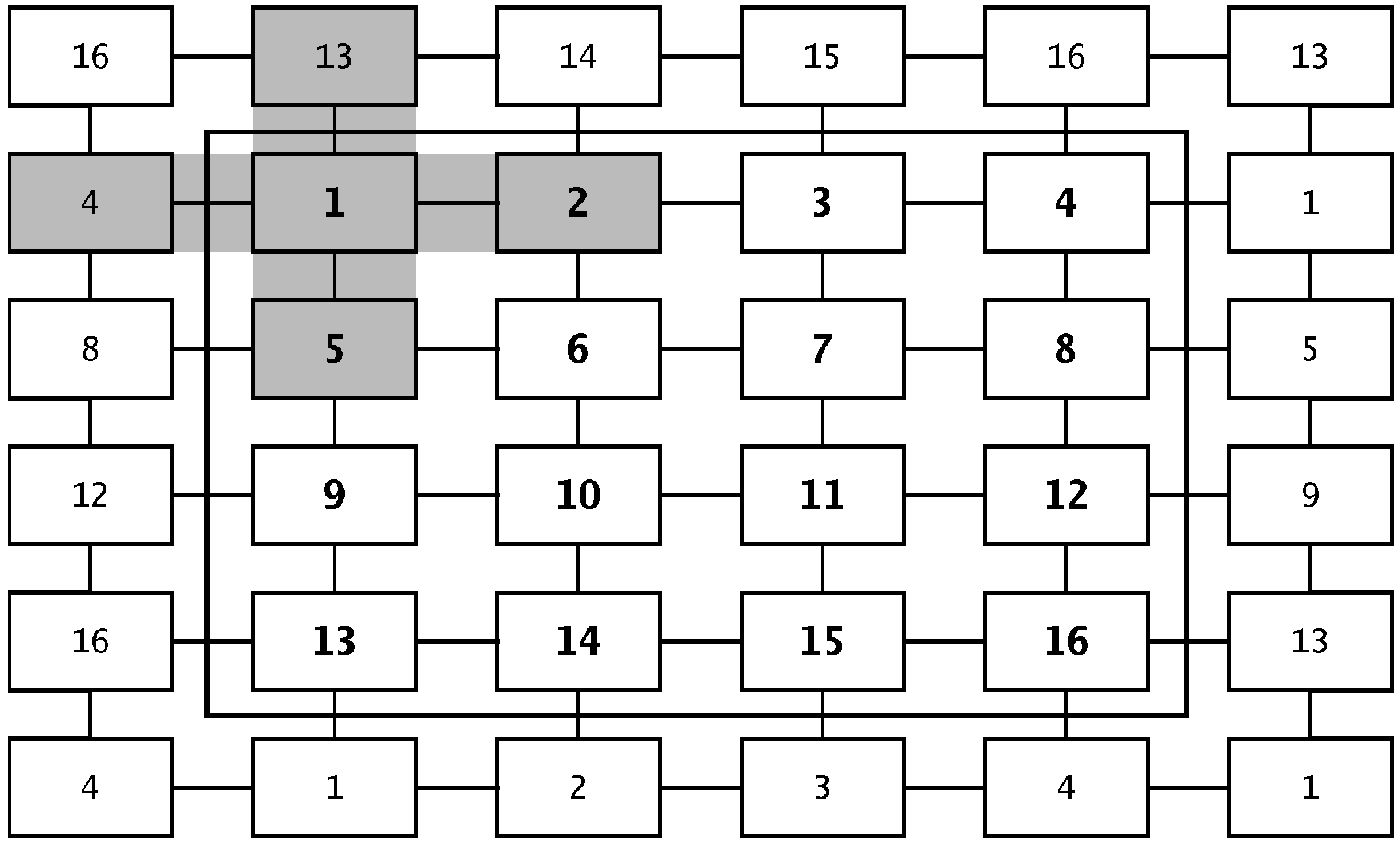
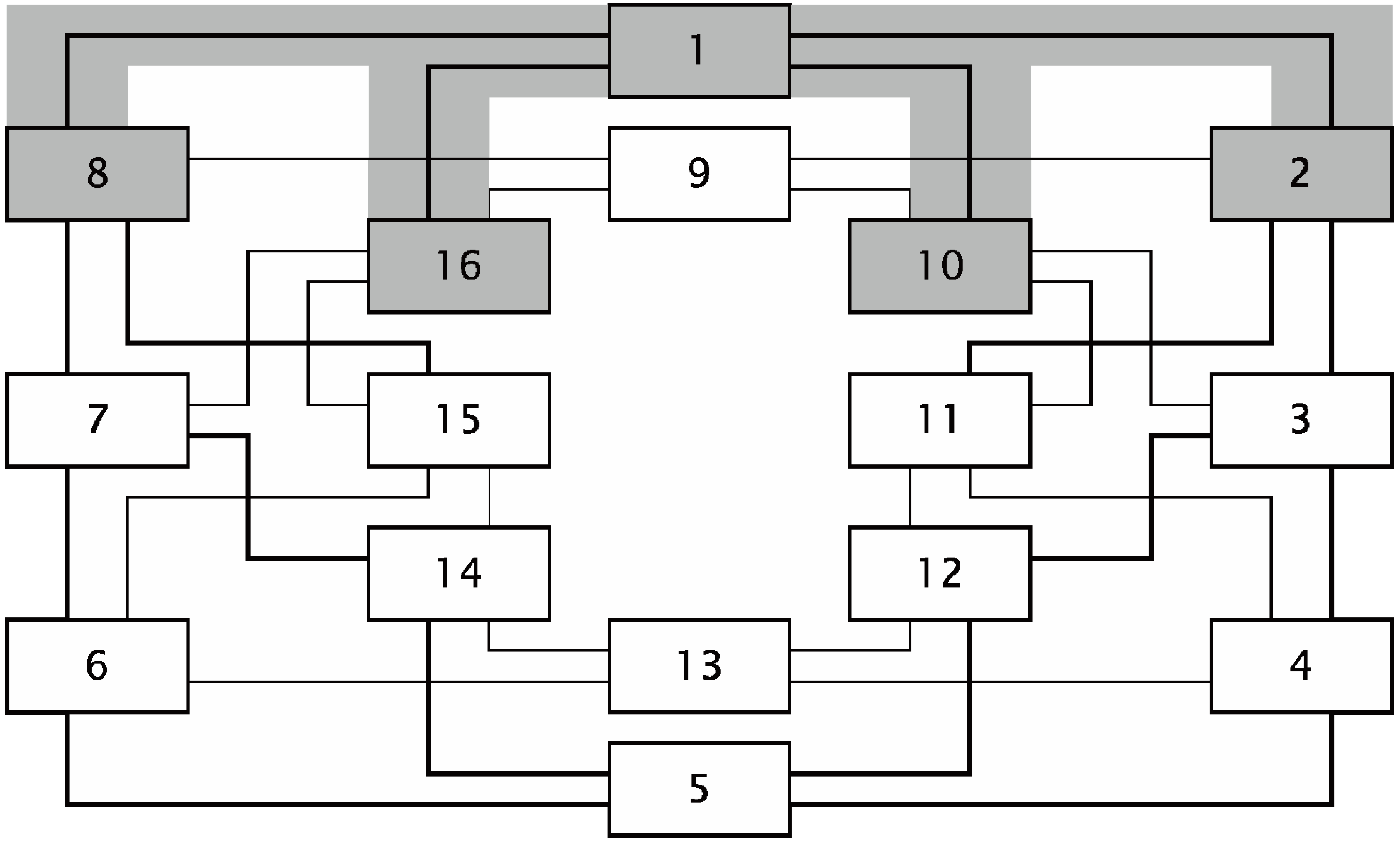
Guided by the findings of Berninghaus et al. [12], where the players’ behavior was affected by different network structures, we used two different structures: a lattice and a circle.

We address our first key question by analyzing how often the players use the ability provided, to play different strategies against their neighbors (to mix strategies within one round).

Comparing the participants’ behavior in the two different network structures, we answer our second key question. Additionally, comparing our observed results with those of SC, we want to provide evidence that learning in networks differs from learning in a random matching environment.

To answer our third key question, we compare our experimental results with the predictions of the five learning concepts. The results of SC were revised in studies by Brunner et al. [13] (henceforth BCG) and by Selten et al. [14]. To ensure that the results are comparable, we use the same statistical techniques as these studies to analyze our data.

As benchmarks for our analyses we use the mean frequencies for each model of learning reported by CGS, the mean frequencies predicted by the equilibrium concepts, and the observed frequencies in the experiment reported by SC. In the study of Chmura et al. [2], the mean frequencies for the models of learning result from the run of simulations.3

As one of our main results we show that learning in networks is different from learning in random matching. However, we find no significant difference between the two network structures. In line with this result, we observe an order of predictive success for the five equilibrium concepts that differs from the order given by SC, which means that learning in networks has a significant impact on the long-run equilibrium, which occurs in the process of learning in networks. This result is supported by our finding regarding the predictions of the four different models of learning. While CGS shows that self-tuning EWA outperformed the other models of learning in random matching, we observe that action-sampling learning best predicts behavior in the network games we used.

As another remarkable result, we find that the majority of players choose the same strategy against each neighbor, i.e., players do not really mix strategies. This holds for both network structures employed in our experiments. Moreover, the average number of players not mixing strategies is slightly higher in the circle network.

2. Description of the Experiment

In our study we use two games (see Figure 1) taken from SC. The main reason we use these games is that they generate clearly distinct predictions for the five equilibrium concepts. Figure 2 shows the theoretical predictions of these concepts for the constant sum game and Figure 3 for the non-constant sum game. Figure 4 (Figure 5) shows the predictions of the four learning models for the constant sum game (non-constant sum game) we relate our experimental results to.4

Figure 1. The constant and the non-constant sum game.

Figure 1. The constant and the non-constant sum game.

Figure 2. Theoretical equilibria in the constant sum games.

Figure 2. Theoretical equilibria in the constant sum games.

Figure 3. Theoretical equilibria in the non-constant sum games.

Figure 3. Theoretical equilibria in the non-constant sum games.

Figure 4. Predictions of the learning models for the constant sum games.

Figure 4. Predictions of the learning models for the constant sum games.

Figure 5. Predictions of the learning models for the non-constant sum games.

Figure 5. Predictions of the learning models for the non-constant sum games.

2.1. The Baseline Games

We use two games, a constant and a non-constant sum game, as baseline games. As explained by SC, both games form a pair that is characterized by having the same best response structure.5

Because we want, on the one hand, to turn the focus to learning by analyzing the impact of different network structures, and on the other hand to refer to the results of SC and BCG, we took the games from SC and extended them to neighborhood games in different network structures.

2.2. The Neighborhood Games and Network Structures

Following Berninghaus et al. [12], we ran the games in exogenously given fixed network structures where each player has four direct neighbors. To accomplish this, 16 players were allocated into two different network structures. The 2 × 2 games described in Section 2.1 represent the baseline games. Based on these games, the neighborhood game was constructed such that each player interacts with her four direct (local) neighbors. Suitably to our first key question, in our experiment each player could use a different strategy against each of her neighbors in each round.

Since it is well known in the literature that network structures affect the players’ behavior in games (see, e.g., [12,15,16]) we used two different structures. Guided by the findings of Berninghaus et al. [12] regarding the behavior of players in a coordination game, we used two different network structures: a lattice and a circle. Figure 6 and Figure 7 provide schematic illustrations of both network structures.

Figure 6. Network structure 1–a lattice.

Figure 6. Network structure 1–a lattice.

Figure 7. Network structure 2–a circle.

Figure 7. Network structure 2–a circle.

It is obvious that in both structures each player interacts with four direct neighbors. The difference between the structures is given by the number of indirect neighbors on the level of indirect interactions.

There might be more equilibria in the network game as we present in Figure 2 and Figure 3. Since we want to compare the players’ behaviors in the two different network structures as well as with the experimental results of SC, we use the equilibria presented in Section 2.1 as benchmarks.

2.3. Exemplary Explanations of the Interaction Structures

In the Lattice (Figure 6), player 1 interacts directly with player 2 as her right, player 4 as her left, player 13 as her top, and player 5 as her bottom neighbor6. On the first level of indirect interactions, player 1 has six indirect neighbors (players 16, 14, 3, 8, 6, and 9). On the second level of indirect interactions, player 1 has four indirect neighbors (players 15, 7, 12, and 10), and one indirect neighbor (player 11) on the third level of indirect interactions.

In the Circle (Figure 7), player 1 interacts directly with player 8 and player 16 as her left neighbors and with player 2 and player 10 as her right neighbors. On the first level of indirect interactions player 1 has five indirect neighbors (players 9, 7, 15, 11, and 3). On the second level of indirect interactions, player 1 has four indirect neighbors (players 6, 14, 12, and 4), and she has two indirect neighbors (players 13 and 5) on the third level of indirect interactions.

3. Experimental Procedure

In order to compare our results with the results of SC, we designed our experiment to be as similar as possible to theirs.

We ran the experiments at the MaXLab, the experimental laboratory at the University of Magdeburg. For each neighborhood game, four sessions were conducted with 16 participants each. The participants were randomly matched on a position in the network. We told them that the matching could (but did not have to) change during the experiment—which did not, in fact, happen. We ran the games over 100 rounds. In each round the players could choose a different strategy against each of the four direct neighbors. After each round the players were informed about the payoffs from each 2 × 2 game, i.e., about the total payoff from the last round and about the accumulated payoffs over all rounds.7

The payoffs were presented by “points” which were converted into Euro at an exchange rate of four payoff points equaling 1 Eurocent. An experimental session lasted about 1 to 1.5 h and the average earnings of a participant were about 10 Euro. The 256 participants in our experiment were recruited using ORSEE software [17] from a pool of mostly students from various faculties. To program our experiments we used the experimental software z-Tree [18].8

4. Experimental Results

To compare our experimental results with the theoretical predictions of the five concepts, and also with the results of SC, in Table 1 we show the observed relative frequencies of playing Up (strategy “up” in the 2 × 2 games) and Left (strategy “left” in the 2 × 2 games), played in the two different network structures.

Table 1. The relative frequencies of playing Up and Left in the baseline games.

Constant Sum Game
		Session 1	Session 2	Session 3	Session 4	Average	Variance
Lattice	Up	0.032	0.053	0.061	0.045	0.048	0.000153
	Left	0.784	0.702	0.587	0.692	0.691	0.006529
Circle	Up	0.036	0.054	0.048	0.059	0.049	0.000098
	Left	0.779	0.683	0.756	0.641	0.715	0.004092
Non-Constant Sum Game
		Session 1	Session 2	Session 3	Session 4	Average	Variance
Lattice	Up	0.062	0.138	0.143	0.100	0.111	0.001425
	Left	0.677	0.764	0.795	0.741	0.744	0.002500
Circle	Up	0.115	0.107	0.110	0.051	0.096	0.000901
	Left	0.724	0.836	0.863	0.672	0.774	0.008223

Table 1. The relative frequencies of playing Up and Left in the baseline games.

Constant Sum Game
		Session 1	Session 2	Session 3	Session 4	Average	Variance
Lattice	Up	0.032	0.053	0.061	0.045	0.048	0.000153
	Left	0.784	0.702	0.587	0.692	0.691	0.006529
Circle	Up	0.036	0.054	0.048	0.059	0.049	0.000098
	Left	0.779	0.683	0.756	0.641	0.715	0.004092
Non-Constant Sum Game
		Session 1	Session 2	Session 3	Session 4	Average	Variance
Lattice	Up	0.062	0.138	0.143	0.100	0.111	0.001425
	Left	0.677	0.764	0.795	0.741	0.744	0.002500
Circle	Up	0.115	0.107	0.110	0.051	0.096	0.000901
	Left	0.724	0.836	0.863	0.672	0.774	0.008223

Key question 1. Do the participants (actually) mix strategies?

Unlike in other studies, the participants in our experiment could choose different strategies against each opponent in each period. Thus, the participants were able to mix their strategies within one round. As shown in Table 2, the participants did not use this opportunity very frequently.

Table 2. Average No. of players choosing the same strategy against each neighbor over 100 rounds.

Average No. of Players Choosing the Same Strategy against Each Neighbor over 100 Rounds
	Lattice	Circle
Constant sum game	81.03%	85.69%
Non-constant sum game	81.16%	86.22%

Table 2. Average No. of players choosing the same strategy against each neighbor over 100 rounds.

Average No. of Players Choosing the Same Strategy against Each Neighbor over 100 Rounds
	Lattice	Circle
Constant sum game	81.03%	85.69%
Non-constant sum game	81.16%	86.22%

The majority of players chose the same strategy for each neighbor. We do not find any difference in the strategy selection for the base games, but there are slight differences between the two different network structures. In terms of learning, or adjusting behavior, the results show that the frequency of choosing the same strategy against each neighbor increases over time (see Table 3).

Table 3. Average No. of players choosing the same strategy in the first fifty and in the second fifty rounds.

Average No. of players choosing the same strategy against each neighbor over rounds 1‑50
	Lattice	Circle
Constant sum game	78.34%	83.06%
Non-constant sum game	76.66%	83.09%
Average No. of players choosing the same strategy against each neighbor over rounds 51‑100
	Lattice	Circle
Constant sum game	83.72%	88.31%
Non-constant sum game	85.66%	89.34%

Table 3. Average No. of players choosing the same strategy in the first fifty and in the second fifty rounds.

Average No. of players choosing the same strategy against each neighbor over rounds 1‑50
	Lattice	Circle
Constant sum game	78.34%	83.06%
Non-constant sum game	76.66%	83.09%
Average No. of players choosing the same strategy against each neighbor over rounds 51‑100
	Lattice	Circle
Constant sum game	83.72%	88.31%
Non-constant sum game	85.66%	89.34%

Result 1. Participants did not mix strategies within one round.

Key question 2. Does the structure of the network affect learning in games?

To find differences in learning between the Lattice network and the Circle network, we first analyze strategy selection in the baseline game. Based on the relative frequencies of playing Up and Left (see Table 1), we find no significant differences between the two network structures (sign test for any level of significance).

We compare our observed results with the experimental results of SC to analyze if there are at least differences between networks as compared to random matching environments with respect to learning behavior. Table 4 shows the observed results.

Table 4. The observed averages of playing Up and Left in games.

	Strategy Choices—Observed Averages in:
	Lattice Network	Circle Network	No Network (SC [1])
		Constant Sum Game
Up	0.048	0.049	0.079
Left	0.691	0.751	0.690
		Non-constant Sum Game
Up	0.111	0.096	0.141
Left	0.744	0.774	0.564

Table 4. The observed averages of playing Up and Left in games.

	Strategy Choices—Observed Averages in:
	Lattice Network	Circle Network	No Network (SC [1])
		Constant Sum Game
Up	0.048	0.049	0.079
Left	0.691	0.751	0.690
		Non-constant Sum Game
Up	0.111	0.096	0.141
Left	0.744	0.774	0.564

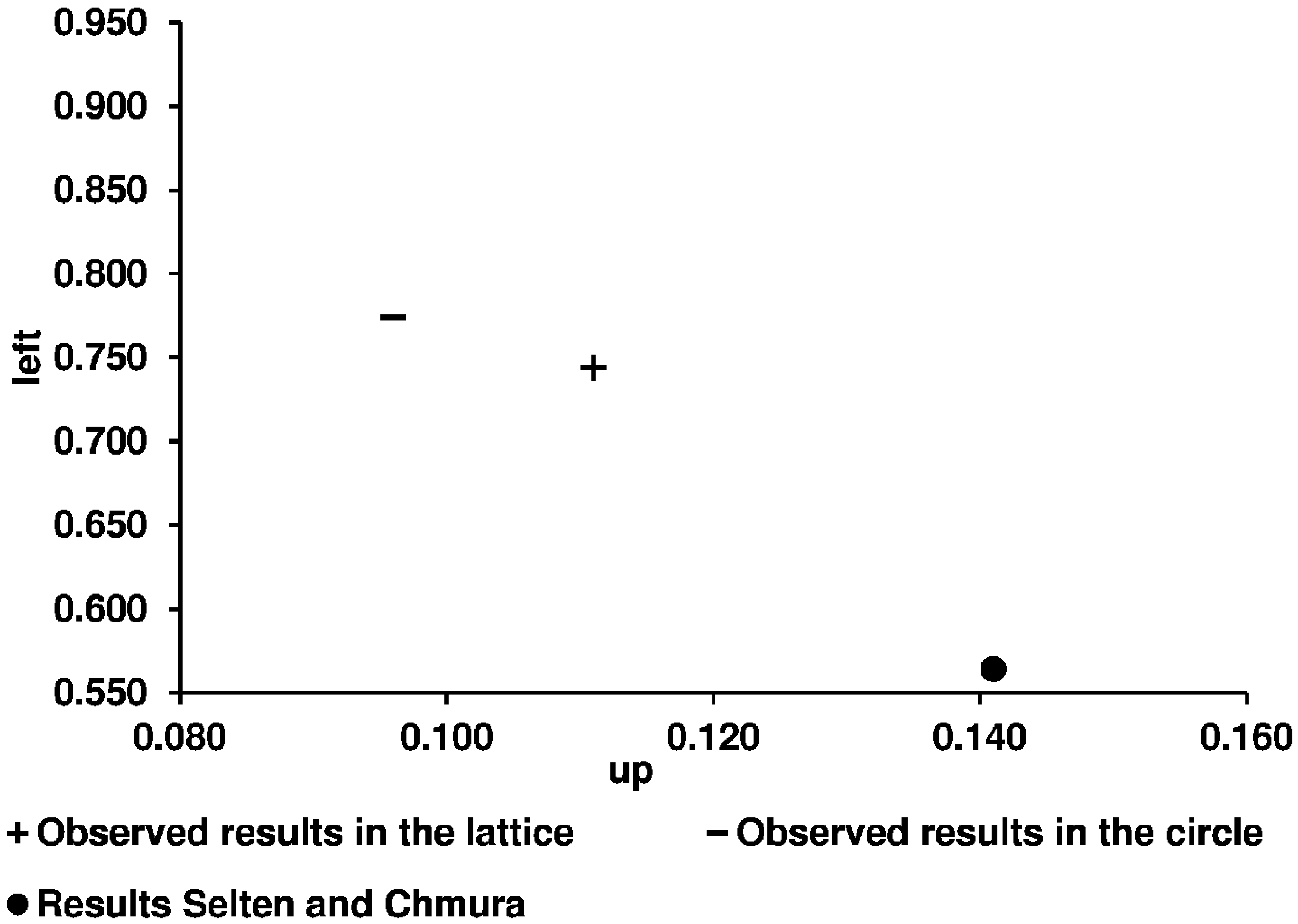
As one can see (Figure 8 and Figure 9), our observed averages for both network structures are different from the results in the 2 × 2 games with only one randomly matched partner. The data in Figure 9 show that this is especially true for the non-constant sum game. These findings imply that learning in networks actually is different from learning in the 2 × 2 random matching environment used by SC.

Figure 8. The observed averages of playing Up and Left in the constant sum game.

Figure 8. The observed averages of playing Up and Left in the constant sum game.

Figure 9. The observed averages of playing Up and Left in the non-constant sum game.

Figure 9. The observed averages of playing Up and Left in the non-constant sum game.

Result 2. We found no significant differences in the participants’ behavior in the two network structures.

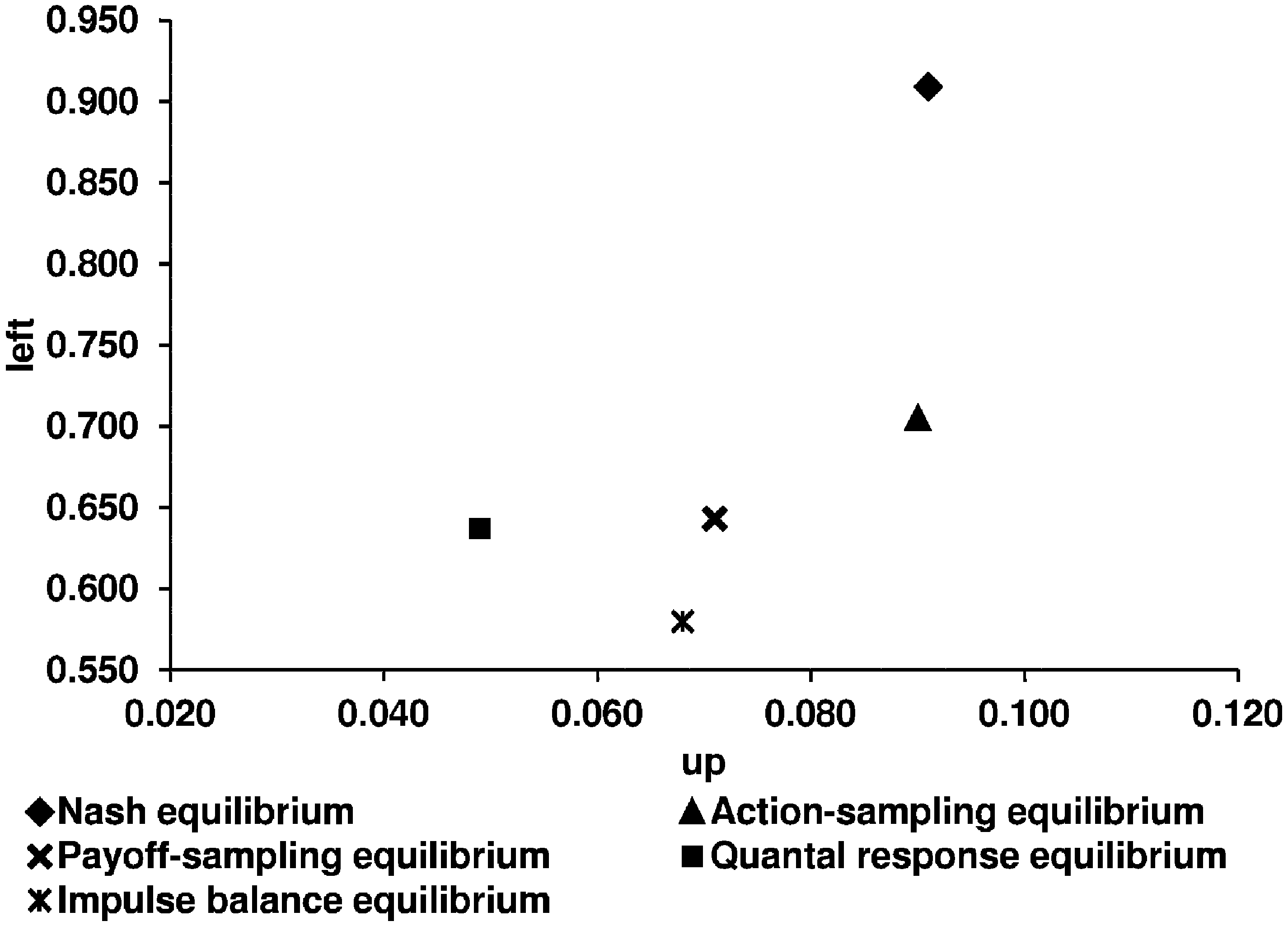
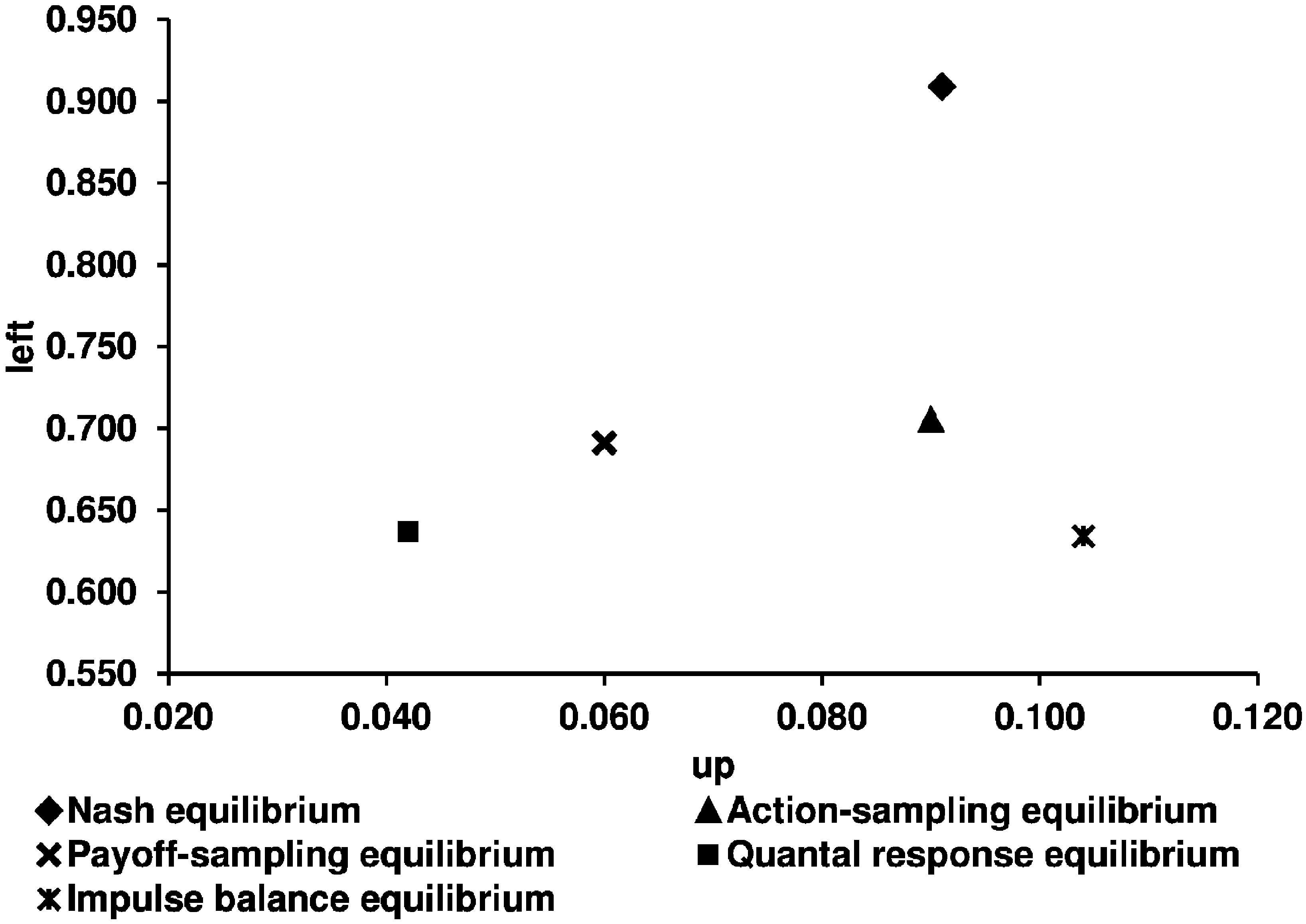
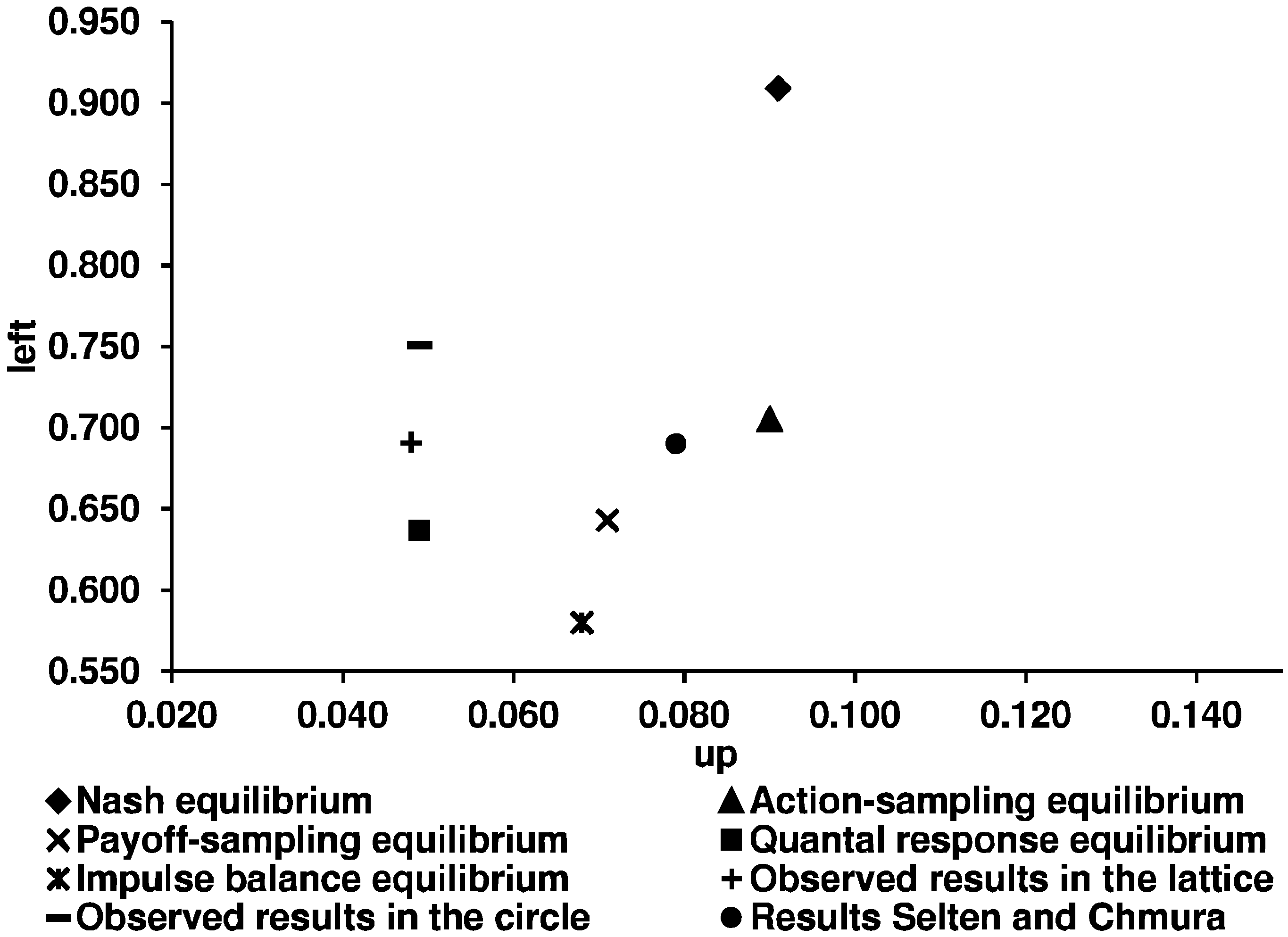
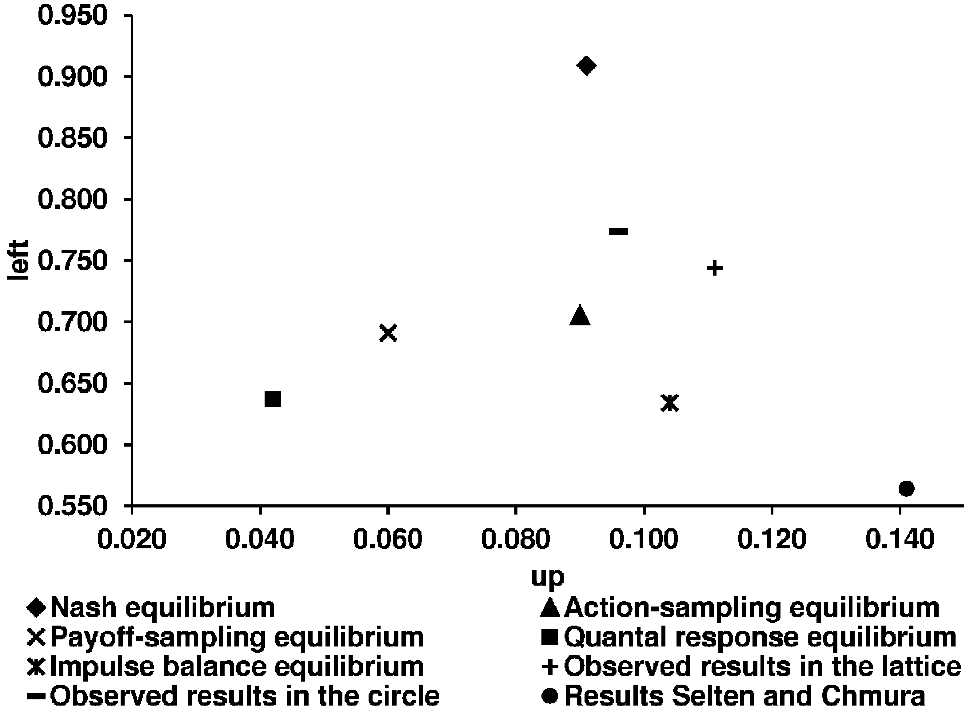
Key question 3. Are the equilibrium concepts tested by Selten and Chmura [1] good predictors for the participants’ behavior in network games?

As we want to answer the question about the predictive success of the five equilibrium concepts in the context of learning in networks, we first illustrate the theoretical predictions of the five concepts and the experimental results (Figure 10 and Figure 11).

Figure 10. Theoretical predictions of the five equilibrium concepts and the experimental results for the constant sum game.

Figure 10. Theoretical predictions of the five equilibrium concepts and the experimental results for the constant sum game.

Figure 11. Theoretical predictions of the five equilibrium concepts and the experimental results for the non-constant sum game.

Figure 11. Theoretical predictions of the five equilibrium concepts and the experimental results for the non-constant sum game.

We use the corrected theoretical predictions of SC, according to BCG. Table 5 shows the corresponding numerical predictions of the five equilibrium concepts.

Table 5. The theoretical predictions of the five equilibrium concepts and the observed relative frequencies of Up and Left strategies.

	Nash	QRE	ASE	PSE	IBE	Observed Average of Selten and Chmura	Our Observed Average in the Lattice	Our Observed Average in the Circle
	Constant sum game
Up	0.091	0.042	0.090	0.071	0.068	0.079	0.048	0.049
Left	0.909	0.637	0.705	0.643	0.580	0.690	0.691	0.751
	Non-constant sum game
Up	0.091	0.042	0.090	0.060	0.104	0.141	0.111	0.096
Left	0.909	0.637	0.705	0.691	0.634	0.564	0.744	0.774

Table 5. The theoretical predictions of the five equilibrium concepts and the observed relative frequencies of Up and Left strategies.

	Nash	QRE	ASE	PSE	IBE	Observed Average of Selten and Chmura	Our Observed Average in the Lattice	Our Observed Average in the Circle
	Constant sum game
Up	0.091	0.042	0.090	0.071	0.068	0.079	0.048	0.049
Left	0.909	0.637	0.705	0.643	0.580	0.690	0.691	0.751
	Non-constant sum game
Up	0.091	0.042	0.090	0.060	0.104	0.141	0.111	0.096
Left	0.909	0.637	0.705	0.691	0.634	0.564	0.744	0.774

To measure the predictive success of the equilibrium concepts, we analyze our data according to the method used by SC. The analysis is based on pairwise comparisons of the observed and the predicted relative frequencies. Table 6 shows the mean squared distances and the sampling variance for both base games played in the two network structures.

Table 6. Mean squared distances of the five equilibrium concepts.

		Nash	QRE	ASE	PSE	IBE	Sampling Variance
Constant sum game	Lattice	0.054297	0.007988	0.006986	0.007880	0.017798	0.005011
	Circle	0.042619	0.009241	0.004899	0.008764	0.021652	0.003143
Non-const. sum game	Lattice	0.030476	0.019173	0.004915	0.008355	0.015144	0.002943
	Circle	0.025158	0.028433	0.011603	0.014969	0.026441	0.006843

Table 6. Mean squared distances of the five equilibrium concepts.

		Nash	QRE	ASE	PSE	IBE	Sampling Variance
Constant sum game	Lattice	0.054297	0.007988	0.006986	0.007880	0.017798	0.005011
	Circle	0.042619	0.009241	0.004899	0.008764	0.021652	0.003143
Non-const. sum game	Lattice	0.030476	0.019173	0.004915	0.008355	0.015144	0.002943
	Circle	0.025158	0.028433	0.011603	0.014969	0.026441	0.006843

Based on the mean squared distances, it can be seen that there is an ordering of the concepts in terms of success: action-sampling equilibrium, payoff-sampling equilibrium, quantal response equilibrium, impulse balance equilibrium, and Nash equilibrium. For the non-constant sum game, the impulse balance equilibrium performs slightly better than the quantal response equilibrium.

Following the analyses in SC and in BCG, we test the results of all 16 independent observations together as well as separately for the constant and the non-constant sum game. Since the theoretical predictions are independent of the network structure, we test the results for both structures together. As in SC, we run the Wilcoxon matched-pairs signed rank test to compare the squared distances of the five concepts from the observed relative frequencies. In Table 7, we show the p-values of a test checking whether the solution concept in the row outperforms the solution concept in the column. The bold numbers in the upper line are the p-values of a test using all 16 observations together. The middle line gives the p-values for the observations in the constant sum game, and the lower line the p-values for the observations in the non-constant game.

As per the remarks in BCG, we also perform the Kolmogorov-Smirnov two-sample test to double-check the significance of the results (p-values are the numbers in brackets given in Table 7).

Table 7. Predictive success-p-values in favor of the row concepts, above: 16 independent observations together, middle: constant sum game (eight independent observations), below: non-constant sum game (eight independent observations).

	PSE	QRE	IBE	Nash
ASE	n. s.	n. s.	2% (10%)	0.001% (0.01%)
	n. s.	n. s.	10% (10%)	0.02% (0.02%)
	n. s.	n. s.	10% (n. s.)	5% (n. s.)
PSE		n. s.	10% (n. s.)	0.05% (2%)
		n. s.	n. s.	0.1% (2%)
		n. s.	n. s.	10% (n. s.)
QRE			n. s.	1% (5%)
			n. s.	0.2% (2%)
			n. s.	n. s.
IBE				5% (10%)
				2% (10%)
				n. s.

Table 7. Predictive success-p-values in favor of the row concepts, above: 16 independent observations together, middle: constant sum game (eight independent observations), below: non-constant sum game (eight independent observations).

	PSE	QRE	IBE	Nash
ASE	n. s.	n. s.	2% (10%)	0.001% (0.01%)
	n. s.	n. s.	10% (10%)	0.02% (0.02%)
	n. s.	n. s.	10% (n. s.)	5% (n. s.)
PSE		n. s.	10% (n. s.)	0.05% (2%)
		n. s.	n. s.	0.1% (2%)
		n. s.	n. s.	10% (n. s.)
QRE			n. s.	1% (5%)
			n. s.	0.2% (2%)
			n. s.	n. s.
IBE				5% (10%)
				2% (10%)
				n. s.

As per the remarks in BCG, we also perform the Kolmogorov-Smirnov two-sample test to double-check the significance of the results (p-values are the numbers in brackets given in Table 7).

When comparing all independent observations, it is obvious that all non-Nash concepts do significantly better than Nash.9

This holds for the constant sum game but not for the non‑constant sum game. Moreover, we found no significant clear order of predictive success among the four non-Nash concepts.

Result 3. There is no significant clear order of predictive success among the four non-Nash concepts.

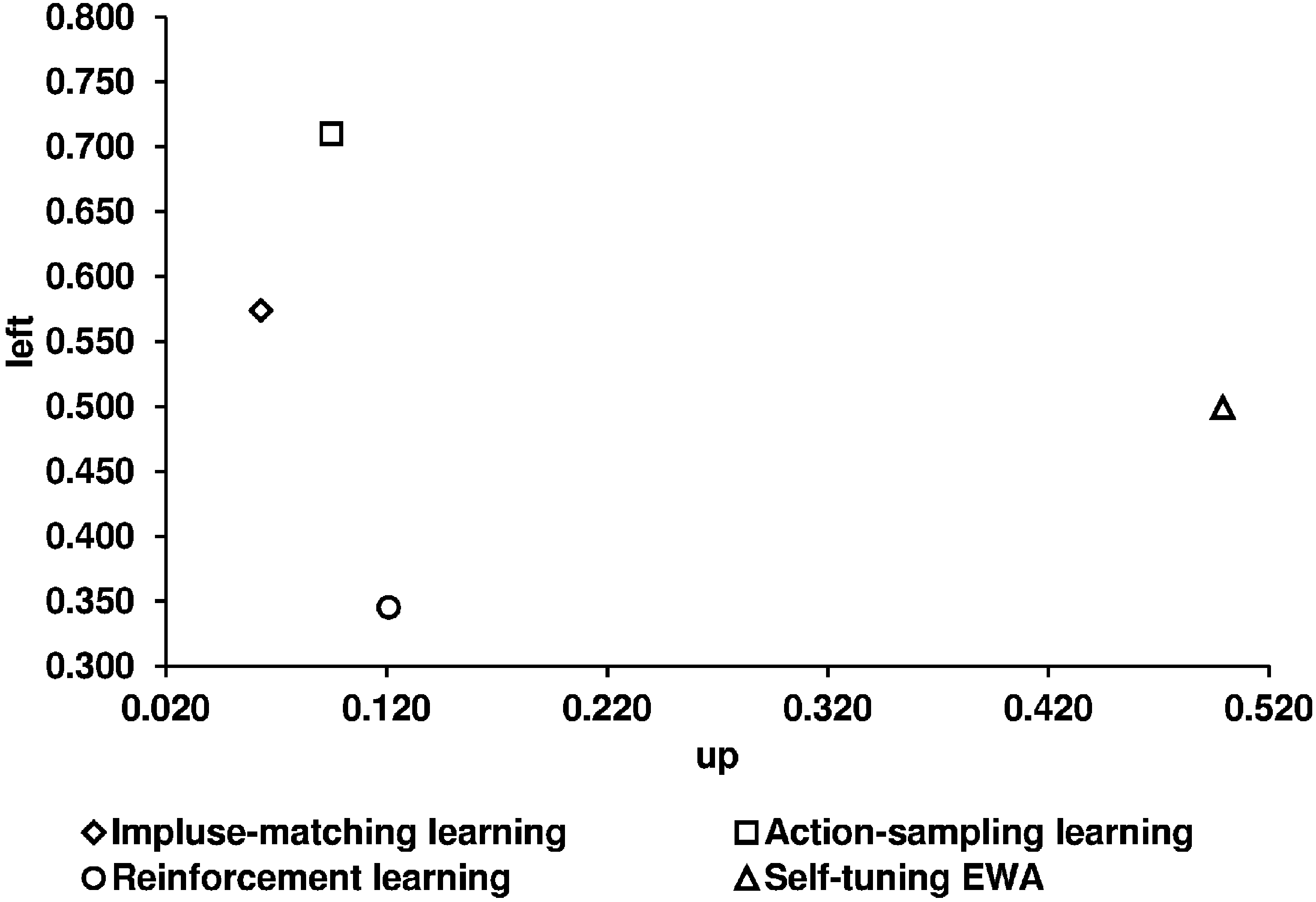
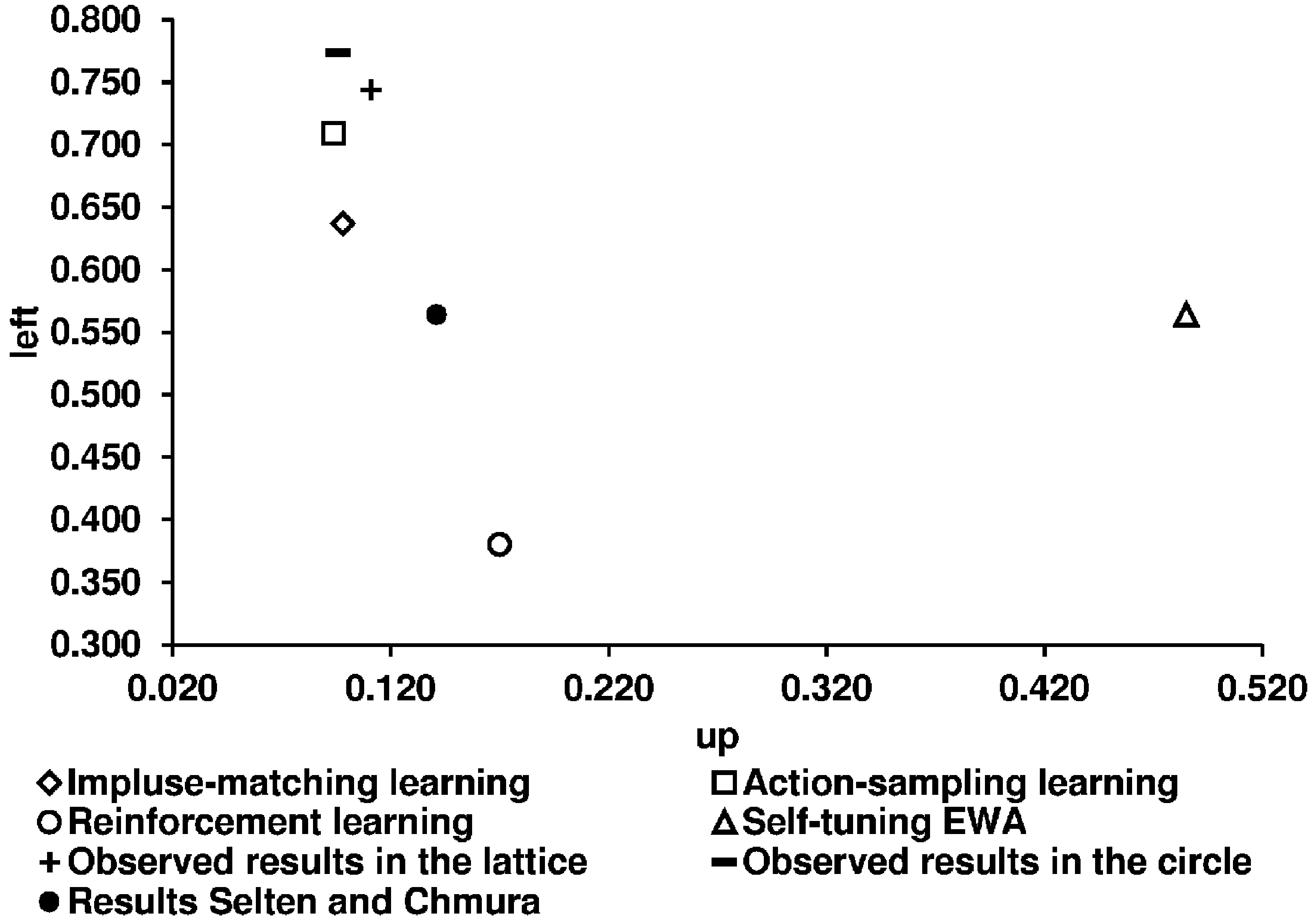
Key question 4. Are the learning models tested by Chmura et al. [2] good predictors for the participants’ learning process in network games?

After analyzing the long-run equilibrium behavior in a learning process, we next concentrate on the round-by-round behavior and relate our observed results to the predictions of the four learning models. We first illustrate the predictions of the four learning models used (given by CGS) and the experimental results (Figure 12 and Figure 13).

Figure 12. Predictions of the four learning models and the experimental results for the constant sum game.

Figure 12. Predictions of the four learning models and the experimental results for the constant sum game.

Figure 13. Predictions of the four learning models and the experimental results for the constant sum game.

Figure 13. Predictions of the four learning models and the experimental results for the constant sum game.

Table 8 shows the corresponding numerical values of the predictions of the four learning models. We use the predictions given by CGS.

Table 8. The predictions of the four learning models and the observed relative frequencies of Up and Left strategies.

	ASL	IML	EWA	REL	Observed Average of Selten and Chmura	Our Observed Average in the Lattice	Our Observed Average in the Circle
	Constant sum game
Up	0.095	0.063	0.499	0.121	0.079	0.048	0.049
Left	0.710	0.574	0.499	0.345	0.690	0.691	0.751
	Non-constant sum game
Up	0.094	0.098	0.485	0.170	0.141	0.111	0.096
Left	0.709	0.637	0.564	0.380	0.564	0.744	0.774

Table 8. The predictions of the four learning models and the observed relative frequencies of Up and Left strategies.

	ASL	IML	EWA	REL	Observed Average of Selten and Chmura	Our Observed Average in the Lattice	Our Observed Average in the Circle
	Constant sum game
Up	0.095	0.063	0.499	0.121	0.079	0.048	0.049
Left	0.710	0.574	0.499	0.345	0.690	0.691	0.751
	Non-constant sum game
Up	0.094	0.098	0.485	0.170	0.141	0.111	0.096
Left	0.709	0.637	0.564	0.380	0.564	0.744	0.774

Based on a pairwise comparison of the observed and the predicted relative frequencies we measure the predictive success of the four learning models. Table 9 shows the mean squared distances and the sampling variances.

Table 9. Mean squared distances of the four learning models.

		IML	ASL	EWA	REL	Sampling Variance
Constant sum game	Lattice	0.007596	0.018992	0.130266	0.245598	0.005011
	Circle	0.005259	0.023143	0.145006	0.251966	0.003143
Non-const. sum game	Lattice	0.004467	0.014609	0.139132	0.175497	0.002943
	Circle	0.011039	0.025549	0.167395	0.202354	0.006843

Table 9. Mean squared distances of the four learning models.

		IML	ASL	EWA	REL	Sampling Variance
Constant sum game	Lattice	0.007596	0.018992	0.130266	0.245598	0.005011
	Circle	0.005259	0.023143	0.145006	0.251966	0.003143
Non-const. sum game	Lattice	0.004467	0.014609	0.139132	0.175497	0.002943
	Circle	0.011039	0.025549	0.167395	0.202354	0.006843

Using the mean squared distances as a measure for predictive success, the following order can be derived: action-sampling learning, impulse-matching learning, reinforcement learning, and self-tuning EWA.

Following the analyses regarding the predictive success of the (long-run) equilibrium concepts, we use the Kolmogorov-Smirnov two-sample test to check for significance of the derived order of predictive success. We test the results for both structures together. Table 10 shows the p-values of the test of all 16 independent observations together as well as separately for the constant and the non-constant sum game. Table 10 is equally structured as Table 7, meaning we show the p-values of a test checking whether the learning model in the row outperforms the learning model in the column.

Table 10. Predictive success-p-values in favor of the row concepts, above: 16 independent observations together, middle: constant sum game (eight independent observations), below: non-constant sum game (eight independent observations).

	IML	REL	EWA
ASL	3.5%	<0.1%	<0.1%
	8.7%	<0.1%	<0.1%
	66.0%	<0.1%	<0.1%
IML		<0.1%	<0.1%
		<0.1%	<0.1%
		<0.1%	<0.1%
REL			0.3%
			0.2%
			8.7%

Table 10. Predictive success-p-values in favor of the row concepts, above: 16 independent observations together, middle: constant sum game (eight independent observations), below: non-constant sum game (eight independent observations).

	IML	REL	EWA
ASL	3.5%	<0.1%	<0.1%
	8.7%	<0.1%	<0.1%
	66.0%	<0.1%	<0.1%
IML		<0.1%	<0.1%
		<0.1%	<0.1%
		<0.1%	<0.1%
REL			0.3%
			0.2%
			8.7%

When comparing all 16 independent observations together, it is obvious that the results of the tests support our derived order of predictive success, i.e., action-sampling learning predicts the round-by-round behavior best. This holds for the constant sum game but not for the non-constant sum game. For the non-constant sum game the predictions of action-sampling learning and impulse-matching learning are not significantly different.

Result 4. There is a significant clear order of predictive success among the four learning models, which is: (1) action-sampling learning, (2) impulse-matching learning, (3) reinforcement learning, and (4) self-tuning EWA.

5. Conclusions

In this paper, we analyzed learning in networks. Therefore, we added network structures to the 2 × 2 games taken from Selten and Chmura [1]. Starting with two different games (a constant and a non‑constant sum game) we construct a neighborhood game with two different network structures (a lattice and a circle), where each player has four direct (local) neighbors. Unlike in other studies, the participants in our experiment could choose a different strategy against each neighbor.

As our study is related to that of SC, we compare our observed results to their experimental results, and to the theoretical predictions of five (long-run) equilibrium concepts (Nash-equilibrium, quantal response equilibrium, action-sampling equilibrium, payoff-sampling equilibrium, and impulse balance equilibrium). We additionally relate our results to the predictions of four learning models (action-sampling learning, impulse-matching learning, reinforcement learning, and self-tuning EWA), used by Chmura et al. [2], to shed some light on the learning process.

Guided by our key questions, we first analyze our data to check if the participants really play mixed strategies. Because the majority of players choose the same strategy against each neighbor, we conclude that the participants did not mix their strategies in a round.

In a second step, we consider the influence of different network structures on the behavior of the participants. The differences between our results and the experimental results of SC provide evidence that learning in network differs from learning in 2 × 2 games with only one randomly matched partner. Unlike in other studies, we find no significant difference in the behavior of the participants in the two network structures we use. We find only slight differences in the number of participants choosing the same strategy against each neighbor.

Concerning our third key question, we show that none of the five equilibrium concepts provides an exact prediction for the participants’ behavior in our experiment. We show that all non-Nash concepts outperform the Nash concept. The order of predictive success of the four non-Nash concepts is different for the constant sum and the non-constant sum game. It is perhaps notable that action-sampling equilibrium and payoff-sampling equilibrium strategies do better than impulse balance equilibrium when both games are combined. Aside from this, there is no clear ranking among these four non-Nash concepts.

With respect to our forth key question, we show that none of the learning models exactly predicts the round-by-round behavior of the participants in our experiment. It becomes obvious, that there is a clear order of predictive success among the four learning models, with action-sampling learning as best and self-tuning EWA as least prediction model. This order is derived when comparing the data of both games together. While this order of predictive success holds for the constant sum game, it does not hold for the non-constant sum game. Here, action-sampling learning predicts as good as impulse-matching learning. However, our derived order of predictive success supports the general findings of CSG using aggregate frequencies.

For future research it looks promising to further develop theories and test different network structures in addition to further replications.